Superresonance Phenomenon from Acoustic Black Holes in Neo-Newtonian theory
Abstract
We explore the possibility of the acoustic analogue of a super-radiance like phenomenon, i.e., the amplification of a sound wave by reflection from the ergo-region of a rotating acoustic black hole in the fluid draining bathtub model in the presence of the pressure be amplified or reduced in agreement with the value of the parameter . We remark that the interval of frequencies depend upon the neo-newtonian parameter () and becomes narrow in this work. As a consequence, the tuning of the neo-newtonian parameter changes the rate of loss of the acoustic black hole mass.
I Introduction
Acoustic black holes possess many of the fundamental properties of the black holes of general relativity and have been extensively studied in the literature M ; Volovik ; fcreation . The connection between black hole physics and the theory of supersonic acoustic flow was established in 1981 by Unruh fcreation and has been developed to investigate the Hawking radiation and other phenomena for understanding quantum gravity. Hawking radiation is an important quantum effect of black hole physics. In 1974, Hawking combining Einstein’s General Relativity and Quantum Mechanics announced that classically a black hole does not radiate, but when we consider quantum effects emits thermal radiation at a temperature proportional to the horizon surface gravity.
Since the Hawking radiation showed by Unruh fcreation is a purely kinematic effect of quantum field theory, we can study the Hawking radiation process in completely different physical systems. For example, acoustic horizons are regions where a moving fluid exceeds the local sound speed through a spherical surface and possesses many of the properties associated with the event horizons of general relativity. In particular, the acoustic Hawking radiation when quantized appears as a flux of thermal phonons emitted from the horizon at a temperature proportional to its surface gravity. Many fluid systems have been investigated on a variety of analog models of acoustic black holes, including gravity wave RS , water Mathis , slow light UL , optical fiber Philbin and electromagnetic waveguide RSch . The models of superfluid helium II Novello , atomic Bose-Einstein condensates Garay ; OL and one-dimensional Fermi degenerate noninteracting gas SG have been proposed to create an acoustic black hole geometry in the laboratory.
The analogous systems employ a classical as well as Newtonian treatment generally, and also some quantum systems are considered. Also, a BH is a relativistic gravitational phenomenon which requires the inertial and gravitational effects of the pressure for a reasonable description of the system. However, relativistic pressure effects can be incorporated in a Newtonian framework in some cases approximatively. This is called neo-Newtonian theory and it is modification of the usual Newtonian theory by comprising the enough pressure into the dynamics.
In the present work, our main goals is firstly to realize the process of drawing the acoustic BH for the neo-Newtonian hydrodynamics, on the other hand, to analyze the impact of neo-Newtonian parameter on the superresonance phenomenon especially on the frequencies of the waves. The paper is organized as follows. In Sec. II we will review the development process of the acoustic BH after recalling the basic concepts of the neo-Newtonian theory ines . In Sec. III we will develop superresonance phenomenon and in Sec. III.2 the numerical results. In Sec. IV we make our final conclusions.
II Newtonian Hydrodynamics in an Expanding Background: Cosmology
In this section, we present the neo-Newtonian hydrodynamics applied to cosmology. However, we consider the standard case of Newtonian equations firstly. In the presence of inviscid perfect fluid, the basic equations of Newtonian hydrodynamics are
| (1) | |||||
| (2) |
where and are fluid density, corresponding pressure and the velocity field, respectively. The dot shows the differentiation with respect to cosmic time . The above system of equations becomes suitable to study cosmology adopting the velocity field (Hubble’s law) where , being the scale factor. It is worth noting the trivial solution for the continuity Eq. (1) , where the today’s scale factor gives the today’s density of the fluid .
Gravitational interaction is coupled into Euler’s equation (2) as
| (3) |
where the gravitational potential obeys the Poisson equation
| (4) |
Eqs. (1) and (3) represents the fluid picture of cosmic medium which is gravitationally self-interacting through Poisson Eq. (4). In the framework of Newtonian cosmology, the Friedmann equations are given as follows
| (5) |
where appears as integration constant associated to the energy of system. Moreover, the pressure does not correspond to homogeneous and isotropic background. With the inclusion of Newtonian cosmology, we can not model a radiation dominated as well as dark energy dominated epoch. This approach is restricted to a description of the Einstein-de Sitter universe.
II.1 Including Pressure: The neo-Newtonian Theory
The neo-Newtonian equations has been developed by McCrea C and Harrison m2 which ensures the effects of pressure as well the simplicity of Newtonian physics. Later, a crucial study related to the perturbative behavior of the neo-Newtonian equations has helped in developing the final expression for the fluid equations in this approach Lima1997 (see also RRRR2003 ; velten ) which are given by
| (6) |
| (7) |
| (8) |
As is widely known, the above set of equations admits a homogeneous and isotropic solution, i.e. , and . In this case, the fluid velocity is (a dot means partial time derivative)
| (9) |
Combining Eqs. (9), (7) and (8), we can obtain the following equations
| (10) | |||
| (11) |
with the continuity equation (6) reducing to the following form
| (12) |
These equations are exactly correspond to the relativistic Friedmann equations. The main idea behind the neo-Newtonian formalism relies on the following substitutions: Firstly, it is necessary to redefine the concept of inertial and passive gravitational mass density. With the redefinition
| (13) |
we rewrite the continuity and the Euler equation.
The second step is the interpretation of the active gravitational mass density i.e., the density that source the gravitational field. Hence the following redefinition
| (14) |
will become the source of the Poisson equation. The generalization of this result in the presence of pressure has been evaluated in C . Moreover, this approach has been modified m2 which leads to neo-Newtonian theory.
When we find the Newtonian equations. The interesting feature of above equations is that the inertial mass present in the Newtonian equation can be replaced by . From cosmological structure formation point of view, it is noted that equation (6) does not provide correct growth of matter for large scale perturbations in the scenario of homogeneous, isotropic and expanding background ademir ; rrrr ; velten . Actually, the correct growth for large scale perturbations is obtained if Eq.(6) is modified as ademir ; rrrr ; velten
| (15) |
This equation shows correspondence with effective metric of usual Newtonian scenario when applied to fluid configuration considered. It represents that one can see, how the neo-Newtonian formulation is sensible to the the specific symmetries and hypothesis of the problem in another context of the cosmological one. This fact may indicate that the construction of a Newtonian counterpart of a relativistic problem may vary from problem to problem, deserving in the general case a deeper analysis.
II.2 Acoustic Black Holes in neo-Newtonian Theory
Let us now consider the barotropic fluid, i.e. , inviscid and irrotational where the equation of state , with and constants. We write the fluid velocity as where is the velocity potential. Thus, we linearise the equations (6), (7) and (15) by perturbing , and as follows:
| (16) | |||||
| (17) | |||||
| (18) | |||||
| (19) |
where is the fluid density, its pressure and its the velocity field. Thus, the wave equation becomes
| (20) |
and we can rewrite as follows
| (21) |
where
| (22) |
Here we are assuming a (2+1)-dimensional spacetime. However, considering the Klein-Gordon equation velten for a massless scalar field we obtain
| (23) |
and so the effective (acoustic) metric, in cylindrical coordinates, reads
| (24) |
where .
II.3 Ergo-region and event horizon
Now considering a static and position independent density, the velocity field is given by
| (25) |
which is a solution obtained from the continuity equation (6) and the velocity potential is
| (26) |
Thus, considering (25), (26) and also the coordinate transformations as follows
| (27) |
being
| (28) |
into the metric (24) we obtain the acoustic black hole in neo-Newtonian theory which is given by ines
| (29) |
where
| (30) | |||||
| (31) |
being the radius of ergo-region and the event horizon, i.e.,
| (32) |
Thus, the metric (29) can be now written in the form
| (36) |
and the inverse of the is
| (40) |
where
| (41) | |||||
| (42) |
III Superresonance phenomenon
III.1 Reflection coefficient
Now, we introduce the metric (36) in the relation Klein Gordon given by
| (43) |
Bearing in mind the stationarity and axisymetry spherical metric (36), we can separate the potential as follows:
| (44) |
where is a real constant (azimuthal number) and the rotational frequency of the acoustic BH. Considering (36), (43), (44), The radial function satisfies the linear second order differential equation
| (45) |
where
| (46) |
| (47) | |||||
| (48) | |||||
| (49) |
and
| (50) |
where
and
| (51) |
Thus, the problem has reduced to a one dimensional Schrödinger problem. Two further analytical simplifications can be made (45): first, We now introduce the tortoise coordinate by using the following equation
| (52) |
which gives the solution
| (53) |
Note that the tortoise coordinate spans the entire real line as opposed to which spans only the half-line; the horizon maps to , while corresponds to . Next, introducing a new radial function . The equation (45) becomes:
| (54) |
with
We remark that the main advantage of the new radial equation (54) over (45) is the absence in the former of a first derivative of the radial function. We analyze differential equation (54) in two distinct radial regions near the horizon, i.e and at asymptote, i.e . In the asymptotic region, Eq.(54) can be written approximately as,
| (55) |
of which one solution is
| (56) | |||||
| (57) |
where is the reflection coefficient. In equation (57), the first term is the incident wave and the second term is the reflected wave. The Wronskian of solution (57) turns out to be
| (58) |
Considering the second field (), the equation (54) becomes:
| (59) | |||||
| (60) |
The physical solution of equation (60) is the following.
where is the transmission coefficient. The Wronskian of solution (LABEL:eq40) is following
| (63) | |||||
| (64) | |||||
| (65) |
Since both equations are actually limiting approximations of the differential Eq. (54), which, as we have mentioned, has a constant Wronskian, it follows that (j , j1 , j2 , j4 )
| (66) |
so that, from (58) and (65), we obtain the relation
| (67) |
superresonance phenomenon occurs when the norm of the reflected wave is greater than the norm of the incident wave, that is, when the reflection coefficient is greater than unity ines1 ; ines2 . Hence, we can observe in eq. (67) that, for frequencies in the range
| (68) |
with
| (69) |
the reflection coefficient has a magnitude larger than unity whose imply the amplification relation of the ingoing sound wave near horizon. with this condition we can extract the energy of the system j4 . It is noteworthy that makes the interval to have superradiance smaller. Here is the azimuthal mode number and is the angular velocity of the usual Kerr-like acoustic BH. the angular velocity of the usual Kerr-like acoustic BH depends of the pressure (parameters and ). Thus, we show that the presence of the the neo-newtonian parameter modifies the quantity of removed energy of the acoustic BH and that is either possible to accentuate or attenuate the amplification of the removed energy of the acoustic. The effect of superresonance can be eliminated when ).
III.2 Numerical results
In order to confirm the effect of pressure on the phenomenon of superresonance, it is necessary to extract the potential energy. The objective in this section, would be to see if the pressure changes the potential energy In this way we obtain the following differential equation for the radial function (45) as
| (70) |
We can rewrite the equation (70) as
| (71) |
where . At this point we introduce the coordinated using the following equation Gamboa
| (72) |
and now introducing the new radial function , we can obtain the following modified radial equation we get to a new radial equation obtained from (71) that reads
| (73) |
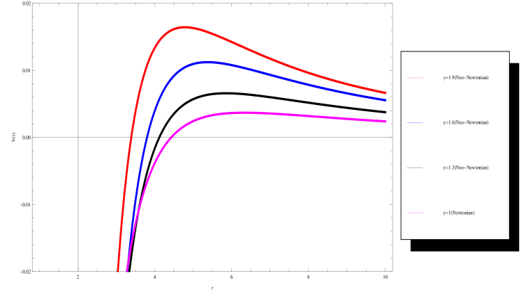
and the potential is given by Dolan ; ABP2012-1
| (74) |
We note that the equation (74) does not satisfy the asymptotic behavior as . We can see from Fig.(1) when the parameter becomes larger, the potential energy increases, which allows us to say that the presence of pressure ascents the phenomenon of superradiance.
One important aspect of the results reported here is that, perhaps, the specific form of the neo-Newtonian equations, retaining the essential features of the relativistic problem, may depend on the symmetries of the problem, as a comparison with the cosmological case suggests. We have constructed acoustic black hole configurations in the context of the neo-Newtonian hydrodynamics. The presence of the parameter in the effective metric of acoustic BHs in the framework of the neo-Newtonian theory is the main feature of our results. This parameter is always larger than if and have the same sign, that is, if the fluid have the expected positive square speed of sound. Hence, essentially, the velocity on the horizon is diminished by the presence of the pressure. It is worth noting that when is equal to , the results of Newtonian theory are recovered M ; fcreation , which leads us to rewrite as follows
| (75) |
The supplementary term is the contribution of the pressure in neo-Newtonian theory.
IV Conclusion
In this paper we shown that the presence of the pressure modify the quantity of removed energy of the acoustic BH and that, it is possible to accentuate or to attenuate the amplification of the removed energy of the acoustic BH and still exists the possibility to cancel the superradiance effect i.e the reflec- tion coefficient is equal to unity, when ) where is the angular velocity of the acoustic black hole. Furthermore, the interval of frequencies becomes narrower in the present scenario. As a consequence, the tuning of the neo-newtonian parameter changes the rate of loss of mass of the acoustic BH.
Acknowledgement: Authors thank Prof. J. C. Fabris and Prof. H. E. S. Velten for useful comments and discussions. Ines G. Salako thanks IMSP for hospitality during the elaboration of this work.
.
References
- (1) M. Visser, Class. Quant. Grav. 15 1767 (1998); [arXiv:gr-qc/9712010].
- (2) G. Volovik, The Universe in a Helium Droplet, (2003) Oxford University Press; L.C. Garcia de Andrade, Phys. Rev. D 70 64004-1 (2004); T. K. Das, Transonic Black Hole Accretion as Analogue System, [arXiv:gr-qc/ 0411006]; G. Chapline and P. O. Mazur, Superfluid Picture for Rotating Space-Times, [arXiv:gr-qc/0407033]. O.K. Pashaev and J.-H. Lee, Theor. Math. Phys. 127, 779, (2001) [arXiv:hep-th/0104258]; S. E. Perez Bergliaffa, K. Hibberd, M. Stone and M. Visser, Physica D191, 121 (2004) [arXiv:cond-mat/0106255]; S. W. Kim, W. T. Kim and J. J. Oh, Phys. Lett. B 608, 10 (2005) [arXiv:gr-qc/0409003]; Xian-Hui Ge, Shao-Feng Wu, Yunping Wang, Guo-Hong Yang and You-Gen Shen, Acoustic black holes from supercurrent tunneling, [arXiv:1010.4961 [gr-qc]]; C. Barcelo, S. Liberati, M. Visser, Analogue gravity, Living Rev. Rel. 8, 12 (2005), [arXiv:gr-qc/0505065].
- (3) W. Unruh, Phys. Rev. Lett. 46, 1351 (1981), -ibid, Phys. Rev. D 51, 2827 (1995), [arXiv:gr-qc/9409008]; L. C. B. Crispino, A. Higuchi, and G. E. A. Matsas, Rev. Mod. Phys. 80, 787 (2008), [arXiv:0710.5373[gr-qc]].
- (4) R. Schützhold and W. G. Unruh, Phys. Rev. D 66, 044019 (2002).
- (5) G. Rousseaux, C. Mathis, P. Maïssa, T. G. Philbin, and U. Leonhardt, New Journal of Physics 10, 053015 (2008).
- (6) U. Leonhardt and P. Piwnicki, Phys. Rev. Lett. 84, 822 (2000); U. Leonhardt, Nature 415, 406 (2002); W. G. Unruh and R. Schützhold, Phys. Rev. D 68, 024008 (2003).
- (7) T. G. Philbin, C. Kuklewicz, S. Robertson, S. Hill, F. König, and U. Leonhardt, Science 319, 1367 (2008).
- (8) R. Schützhold and W. G. Unruh, Phys. Rev. Lett. 95, 031301 (2005).
- (9) M. Novello, M. Visser and G. Volovik (Eds.), Artificial Black Holes, World Scientific, Singapore, (2002).
- (10) L. J. Garay, J. R. Anglin, J. I. Cirac, and P. Zoller, Phys. Rev. Lett. 85, 4643 (2000).
- (11) O. Lahav, A. Itah, A. Blumkin, C. Gordon and J. Steinhauer, [arXiv0906.1337].
- (12) S. Giovanazzi, Phys. Rev. Lett. 94, 061302 (2005).
- (13) J. C. Fabris, O. F. Piattella, I. G. Salako, J. Tossa, H. E. S. Velten MPL A 28, 1350169(2013) arXiv:1308.1859.
- (14) W. H. McCrea, Proc. R. Soc. London 206, 562 (1951).
- (15) E. R. Harrison, Ann. Phys (N.Y.) 35, 437 (1965).
- (16) J.A.S. Lima, V. Zanchin and R. Brandenberger, Month. Not. R. Astron. Soc. 291, L1 (1997).
- (17) R.R.R. Reis, Phys. Rev. D67, 087301 (2003); erratum-ibid D68, 089901(2003).
- (18) J.A.S. Lima, V. Zanchin and R. Brandenberger, MNRAS, 291, L1-L4 (1997).
- (19) R.R.R. Reis, Phys. Rev. D67, 087301 (2003); erratum-ibid D68, 089901 (2003).
-
(20)
H. Velten, D. J. Schwarz, J. C. Fabris and W. Zimdahl, Phys Rev D 88, 103522 (2013).
A. M. Oliveira, H. E. S. Velten, J. C. Fabris, I. G. Salako, Eur. Phys. J. C 74 3170 (2014) - (21) B. DeWitt, Phys. Rep. 6, 295 (1975).
- (22) M. A. Anacleto, F. A. Brito and E. Passos Phys.Lett.B 703:609-613,2011
- (23) Geusa de A. Marques arXiv:0705.3916v1 [gr-qc]
- (24) S. Basak and P. Majumdar, Class. Quant. Grav. 20, 3907 (2003).
- (25) A. Starobinski, Sov. Phys. JETP 7, 28 (1973).
- (26) B. DeWitt, Phys. Rep. 6, 295 (1975).
- (27) J. Gamboa and F. Mendez, Class. Quant. Grav. 18, 225 (2001), [hep-th/0006020]
- (28) S. Deser and R. Jackiw R, Commun. Math. Phys. 118, 495 (1988).
- (29) S.R. Dolan, E.S. Oliveira, L.C.B. Crispino, Phys. Lett. B 701, 485 (2011).
- (30) M. A. Anacleto, F. A. Brito and E. Passos, Phys. Rev. D 86, 125015 (2012) [arXiv:1208.2615 [hep-th]]; Phys. Rev. D 87, 125015 (2013) [arXiv:1210.7739 [hep-th]]; M. A. Anacleto, F. A. Brito and E. Passos, Phys. Lett. B 743, 184 (2015)