New Extended Formulations of Euler-Korteweg Equations
Based on a Generalization of the Quantum Bohm Identity

Abstract

In this note, we propose an original extended formulation of Euler-Korteweg systems based on a generalization of the quantum Bohm potential identity. This new formulation allows to propose a useful construction of a numerical scheme with entropy stability property under a hyperbolic CFL condition. We also comment the use of the identity for compressible Navier-Stokes equations with degenerate viscosities.

Résumé Généralisation de l’identité de Bohm quantique et nouvelles formulations augmentées pour équations d’Euler-Korteweg. Dans cette note, on propose une formulation augmentée originale des systèmes d’Euler-Korteweg basée sur une généralisation de l’identité dite du potentiel de Bohm quantique . La motivation principale est la construction de schémas avec stabilité entropique sous condition CFL hyperbolique du système d’Euler-Korteweg. On présente également quelques commentaires concernant l’utilisation de cette identité dans le cadre des équations de Navier–Stokes avec viscosités dégénérées.

, , ,

Received *****; accepted after revision +++++
Presented by

Version française abrégée

Dans cette note, nous introduisons de nouvelles formulations augmentées (sous forme conservative) du système d’Euler-Korteweg (1)–(3) en plusieurs dimensions d’espace. Selon le choix des coefficients de capillarité, ce type de système intervient dans la modélisation des mélanges de type liquide-vapeur, des super-fluides ou de l’hydrodynamique quantique par exemple. Nous nous intéressons ici à de nouvelles formulations permettant de construire un schéma numérique à stabilité entropique. Nous étendons ainsi les travaux récents de deux des auteurs qui considéraient le cas uni-dimensionnel. Nous traitons les termes dispersifs implicitement et donnons un résultat de stabilité entropique des schémas d’ordre 1 sous condition CFL hyperbolique. A titre d’illustration, nous présentons des résultats numériques pour des films minces avec tension de surface modélisés par les équations de Saint-Venant.

1 Introduction

In this paper, we introduce (new) extended formulations of the so-called Euler Korteweg system which, in several space dimensions, reads

$$\displaystyle\partial_{t}\varrho + {\rm div}(\varrho{\bf u})=0,$$ (1)

$$\displaystyle\partial_{t}(\varrho{\bf u}) + {\rm div}(\varrho{\bf u}\otimes{\bf u})+\nabla p(\varrho)={\rm div}(\mathbf{K}),$$ (2)

where $\varrho$ denotes the fluid density, ${\bf u}$ the fluid velocity, $p(\varrho)$ the fluid pressure and $\mathbf{K}$ the Korteweg stress tensor defined as

$$\mathbf{K}=\left(\varrho{\rm div}(K(\varrho)\nabla\varrho)+\frac{1}{2}(K(\varrho)-\varrho K^{\prime}(\varrho))|\nabla\varrho|^{2}\right)\mathbf{I}_{\mathbb{R}^{n}}-K(\varrho)\nabla\varrho\otimes\nabla\varrho.$$ (3)

with $K(\varrho)$ the capillary coefficient. These models comprise liquid-vapor mixture (for instance highly pressurized and hot water in nuclear reactors cooling system) [7], superfluids (Helium near absolute zero) [6] or even regular fluids at sufficiently small scales (think of ripples on shallow waters) [8]. In quantum hydrodynamic, the capillary coefficient is chosen so that $\varrho K(\varrho)=constant$: in this case; the Euler-Korteweg equations correspond to the nonlinear Schrödinger equation after Madelung transform. In classical fluid mechanics, the capillary coefficient $K(\varrho)$ is chosen constant.

The system (1)–(2) admits two additional conservations laws. One conservation law is satisfied by the fluid velocity

$$\partial_{t}{\bf u}+{\bf u}\cdot\nabla\,{\bf u}+\nabla(\delta\mathcal{E})=0,$$ (4)

with $\mathcal{E}$ the potential energy and $\delta\mathcal{E}$ its variational gradient

$$\mathcal{E}(\varrho,\nabla\varrho)=F_{0}(\varrho)+\frac{1}{2}K(\varrho)|\nabla\varrho|^{2},\quad\delta\mathcal{E}=F^{\prime}_{0}(\varrho)-\frac{1}{2}K^{\prime}(\varrho)|\nabla\varrho|^{2}-K(\varrho)\Delta\varrho.$$ (5)

The local existence of strong solution to (1), (4) is proved in [1]. For that purpose, the authors introduced an extended formulation by considering an additional velocity ${\bf w}=\nabla\varphi(\varrho)$ with $\sqrt{\varrho}\varphi^{\prime}(\varrho)=\sqrt{K(\varrho)}$:

$$\partial_{t}{\bf u}+{\bf u}\cdot\nabla\,{\bf u}+\nabla\left(F^{\prime}_{0}(\varrho)-\frac{|{\bf w}|^{2}}{2}\right)=\nabla\left(a(\varrho){\rm div}({\bf w})\right),\quad\partial_{t}{\bf w}+\nabla\left({\bf u}^{T}\,{\bf w}\right)=-\nabla\left(a(\varrho){\rm div}({\bf u})\right),$$

where $a(\varrho)=\sqrt{K(\varrho)\varrho}$. This formulation is particularly adapted to the derivation of a priori estimates, the very first one being a conservation law on the total (kinematic+potential) energy :

$$\displaystyle\partial_{t}\left(\frac{\varrho}{2}|{\bf u}|^{2}+\mathcal{E}(\varrho,\nabla\varrho)\right)+{\rm div}\left({\bf u}\left(\frac{\varrho}{2}|{\bf u}|^{2}+\mathcal{E}(\varrho,\nabla\varrho)+p(\varrho)\right)\right)={\rm div}\Bigl{(}F(\varrho)(\nabla{\bf w}\,{\bf u}-\nabla{\bf u}\,{\bf w})\Bigr{)}$$

$$-{\rm div}\Bigl{(}(F(\varrho)-\varrho F^{\prime}(\varrho))({\rm div}({\bf w}){\bf u}-{\rm div}({\bf u}){\bf w})\Bigr{)}.$$ (6)

with $F^{\prime}(\varrho)=\varrho\varphi^{\prime}(\varrho)$.

In this note, we introduce a new extended formulation of (1)–(2) by considering the conservative variables $\varrho{\bf u},\varrho{\bf w}$ instead of ${\bf u},{\bf w}$. The key point is the generalization of the quantum potential Bohm identity. It allows to transform the Euler-Korteweg system into a hyperbolic system perturbed by a second order skew symmetric term. The main motivation is the construction of a numerical scheme which is easily proved “entropy” stable. Two of the authors performed this approach in a one dimensional setting and proved entropy stability under “capillary” Courant-Friedrichs-Lewy (denoted CFL in the sequel) condition [9]. Here, we extend this approach to the multi-dimensional setting. Moreover, in order to avoid restrictive CFL condition, we treat dispersive terms implicitely and prove entropy stability of first order schemes under a hyperbolic CFL condition. We present preliminary numerical results for thin films with surface tension modeled by the shallow water equations.

2 Generalization of the quantum Bohm identity and extended formulation

Let us first present an extension of the quantum potential Bohm identity

$$2\varrho{\rm div}\bigl{(}\Delta\sqrt{\varrho}/\sqrt{\varrho}\bigr{)}={\rm div}\Bigl{(}\varrho\nabla\nabla\log\varrho\Bigr{)}$$

strongly used in quantum fluid mechanics. More precisely, we can prove after some algebraic calculations the following relation

$$\varrho\nabla\bigl{(}\sqrt{K(\varrho)}\,\Delta(\int_{0}^{\varrho}\sqrt{K(s)}\,ds)\bigr{)}={\rm div}\Bigl{(}F(\varrho)\nabla\nabla\varphi(\varrho)\Bigr{)}-\nabla\Bigl{(}\bigl{(}F(\varrho)-F^{\prime}(\varrho)\varrho\bigr{)}\Delta\varphi(\varrho)\Bigr{)}$$ (7)

with $\sqrt{\varrho}\varphi^{\prime}(\varrho)=\sqrt{K(\varrho)}$, $F^{\prime}(\varrho)=\sqrt{K(\varrho)\,\varrho}$. This relation is a non trivial extension of the quantum Bohm identity which corresponds to the case $K(\varrho)=c/\varrho$. Remark that the left–hand side of (7) corresponds to the capillarity term $K(\varrho)|\nabla\varrho|^{2}/2$. It suffices to observe that

$$K(\varrho)|\nabla\varrho|^{2}=|\nabla(\int_{0}^{\varrho}\sqrt{K(s)})\,ds|^{2}$$

and thus as observed in [2] the variational gradient of the potential energy may be written

$$\delta\mathcal{E}=F^{\prime}_{0}(\varrho)-\bigl{(}\sqrt{K(\varrho)}\,\Delta(\int_{0}^{\varrho}\sqrt{K(s)}\,ds)\bigr{)}.$$

Following now the strategy of [1], we introduce a “good” additional unknown, homogeneous to a velocity. We denote this additional velocity ${\bf w}=\nabla\varphi(\varrho)$ with $\sqrt{\varrho}\varphi^{\prime}(\varrho)=\displaystyle\sqrt{K(\varrho)}$. In order to write a suitable extended formulation of the Euler Korteweg model, we also define $F(\varrho)$ so that $F^{\prime}(\varrho)=\sqrt{K(\varrho)\varrho}$. The Euler Korteweg system admits the extended formulation

$$\left\{\begin{array}[]{l}\vspace{0.2cm}\partial_{t}\varrho+{\rm div}(\varrho\,{\bf u})=0,\\ \vspace{0.2cm}\partial_{t}(\varrho\,{\bf u})+{\rm div}(\varrho{\bf u}\otimes{\bf u})+\nabla p(\varrho)={\rm div}(F(\varrho)\nabla{\bf w}^{T})-\nabla\left((F(\varrho)-\varrho F^{\prime}(\varrho)){\rm div}({\bf w})\right),\\ \vspace{0.2cm}\partial_{t}(\varrho\,{\bf w})+{\rm div}(\varrho{\bf w}\otimes{\bf u})=-{\rm div}(F(\varrho)\nabla{\bf u}^{T})+\nabla\left((F(\varrho)-\varrho F^{\prime}(\varrho)){\rm div}({\bf u})\right),\end{array}\right.$$ (8)

The total energy is then transformed into a classical entropy of the first order part of (8)

$$\frac{\varrho}{2}\|{\bf u}\|^{2}+\mathcal{E}(\varrho,\nabla\varrho)=\frac{\varrho}{2}\left(\|{\bf u}\|^{2}+\|{\bf w}\|^{2}\right)+F_{0}(\varrho):={\bar{\mathcal{E}}}(\varrho,{\bf u},{\bf w}),$$

whereas the second order part is skew symmetric. As a consequence, the energy conservation law (6) is obtained through a similar computation than in the first order case.

Remark. Note that our formulation may be coupled to the result recently obtained in [5] to write an augmented formulation to the following compressible Navier–Stokes system with drag and capillary terms

$$\displaystyle\partial_{t}\varrho + {\rm div}(\varrho{\bf u})=0,$$ (9)

$$\displaystyle\partial_{t}(\varrho{\bf u}) + {\rm div}(\varrho{\bf u}\otimes{\bf u})-2{\rm div}(\mu(\varrho)D({\bf u})-\nabla(\lambda(\varrho){\rm div}{\bf u})+\nabla p(\varrho)+r_{1}\varrho|u|^{\alpha}u={\rm div}(\mathbf{K}),$$ (10)

if $\lambda(\varrho)=2(\mu^{\prime}(\varrho)\varrho-\mu(\varrho))$ and $K(\varrho)=c(\mu^{\prime}(\varrho))^{2}/\varrho$. Such compatible system could be used to prove global existence of weak solutions to the compressible Navier-Stokes equations with degenerate viscosities without capillary and drag terms. It has been recently performed in [10] in the case $\mu(\varrho)=\mu\varrho$ and $\lambda(\varrho)=0$ introducing the quantum capillary term namely with $K(\varrho)=c/\varrho$.

3 Application: stable schemes under hyperbolic CFL condition

In this section, we introduce a numerical scheme for (8). The numerical domain is a rectangle defined by $0\leq x\leq L_{x}$ and $0\leq y\leq L_{y}$, which is divided into $N=n_{x}\times n_{y}$ rectangular cells. For the sake of simplicity, we consider uniform grid with constant spatial steps $\delta x$ and $\delta y$. We focus on the spatial discretization of the second order terms: they are written as $\displaystyle\partial_{\alpha}(f(\varrho)\partial_{\beta}u)$ with $(\alpha,\beta)\in\{x,y\}$ and $f(\varrho)=F(\varrho),\varrho F^{\prime}(\varrho),F(\varrho)-\varrho F^{\prime}(\varrho)$. For that purpose, we introduce the following finite difference operators:

$$\begin{array}[]{ll}\displaystyle(d_{1}u)_{i,j}=\frac{u_{i+1/2,j}-u_{i-1/2,j}}{\delta x},\quad(d_{1}^{+}u)_{i+1/2,j}=\frac{u_{i+1,j}-u_{i,j}}{\delta x},\quad({\bar{d}}_{1}u)_{i,j}=\frac{u_{i+1,j}-u_{i-1,j}}{2\delta x},\\ \displaystyle(d_{2}u)_{i,j}=\frac{u_{i,j+1/2}-u_{i,j-1/2}}{\delta y},\quad(d_{2}^{+}u)_{i,j+1/2}=\frac{u_{i,j+1}-u_{i,j}}{\delta y},\quad({\bar{d}}_{2}u)_{i,j}=\frac{u_{i,j+1}-u_{i,j-1}}{2\delta y}.\end{array}$$ (11)

As a result the differential operator $\displaystyle\mathcal{T}(\varrho){\bf u}={\rm div}(F(\varrho)\nabla{\bf u}^{T})+\nabla\left((\varrho F^{\prime}(\varrho)-F(\varrho)){\rm div}({\bf u})\right)$ is approximated by $\mathcal{T}_{h}(\varrho)$ defined as

$$\mathcal{T}_{h}(\varrho){\bf u}_{i,j}=\left\{\begin{array}[]{ll}\displaystyle d_{1}\left(\varrho\,F^{\prime}(\varrho)d_{1}^{+}{\bf u}_{1}\right)_{i,j}+{\bar{d}}_{2}\left(F(\varrho){\bar{d}}_{1}{\bf u}_{2}\right)_{i,j}+{\bar{d}}_{1}\left((\varrho F^{\prime}(\varrho)-F(\varrho)){\bar{d}}_{2}{\bf u}_{2}\right)_{i,j},\\ \displaystyle{\bar{d}}_{1}\left(F(\varrho){\bar{d}}_{2}{\bf u}_{1}\right)_{i,j}+{\bar{d}}_{2}\left((\varrho F^{\prime}(\varrho)-F(\varrho)){\bar{d}}_{1}{\bf u}_{1}\right)_{i,j}+d_{2}\left(\varrho F^{\prime}(\varrho)d_{2}^{+}{\bf u}_{2}\right)_{i,j}\end{array}\right.$$

We discretize (8) as follows

$$\left\{\begin{array}[]{l}\vspace{0.2cm}\frac{\varrho_{i,j}^{n+1}-\varrho_{i,j}^{n}}{\delta t}+d_{1}(\mathcal{F}_{\varrho,1}^{n})_{i,j}+d_{2}(\mathcal{F}_{\varrho,2}^{n})_{i,j}=0,\\ \vspace{0.2cm}\frac{(\varrho\,{\bf u})_{i,j}^{n+1}-(\varrho{\bf u})_{i,j}^{n}}{\delta t}+d_{1}({\bf\mathcal{F}}_{{\bf u},1}^{n})_{i,j}+d_{2}({\bf\mathcal{F}}_{{\bf u},2}^{n})_{i,j}=\mathcal{T}_{h}(\varrho^{n+1}){\bf w}^{n+1}_{i,j},\\ \vspace{0.2cm}\frac{(\varrho{\bf w})_{i,j}^{n+1}-(\varrho{\bf w})_{i,j}^{n}}{\delta t}+d_{1}({\bf\mathcal{F}}_{{\bf w},1}^{n})_{i,j}+d_{2}({\bf\mathcal{F}}_{{\bf w},2}^{n})_{i,j}=-\mathcal{T}_{h}(\varrho^{n+1}){\bf u}^{n+1}_{i,j},\end{array}\right.$$ (12)

where $\mathcal{F}_{\varrho,k}^{n},{\bf\mathcal{F}}_{{\bf u},k}^{n},{\bf\mathcal{F}}_{{\bf w},k}^{n}$ ($k=1,2$) are classical Rusanov fluxes evaluated at $\varrho^{n},{\bf u}^{n},{\bf w}^{n}$. More precisely, the convection part is treated explicitly whereas the capillary terms are treated implicitly. Remark that there are no capillary terms in the mass conservation law so that the implicit step amounts to solve a linear sparse system and is easily proved entropy stable. As a consequence, one can prove, by using discrete duality properties of the discrete second order operators, the following entropy stability result.

Theorem 3.1

Suppose (12) is completed with periodic boundary conditions. Assume the hyperbolic scheme (system (12) with $F=0$) is entropy stable then the fully hyperbolic/capillary scheme (12) is entropy stable:

$$\sum_{i=0}^{n_{x}}\sum_{j=0}^{n_{y}}{\bar{\mathcal{E}}}(\varrho_{i,j}^{n+1},{\bf u}_{i,j}^{n+1},{\bf w}_{i,j}^{n+1})\leq\sum_{i=0}^{n_{x}}\sum_{j=0}^{n_{y}}{\bar{\mathcal{E}}}(\varrho_{i,j}^{n},{\bf u}_{i,j}^{n},{\bf w}_{i,j}^{n}).$$

This means that the numerical scheme (12) is entropy stable under a classical hyperbolic Courant-Friedrichs-Lewy condition. As an application, we carried out a numerical simulation of a thin film falling down an inclined plane. A consistent shallow water model [3] is given by

$$\displaystyle\partial_{t}h+{\rm div}\,(h\mathbf{u}\,) = 0,$$ (13)

$$\displaystyle\partial_{t}(h\mathbf{u})+{\rm div}\left(h\,\mathbf{u}\otimes\,\mathbf{u}\right)+\nabla(p(h))+\left(\frac{g\sin(\theta)}{\nu}\right)^{2}\,\partial_{x}\left(\frac{2h^{5}}{225}\right)\mathbf{e}_{1} = S(h,{\bf u})+\frac{\sigma h}{\rho}\nabla(\Delta h).$$ (14)

with $p(h)=\displaystyle g\cos(\theta)h^{2}/2$ and $\displaystyle S(h,{\bf u})=gh\sin(\theta)\mathbf{e}_{1}-3{\nu\mathbf{u}}/{h}$ and ${\bf e}_{1}$ the first vector of the canonical base directed downstream. Here $g=9.8$ is the gravity constant, $\rho,\nu,\sigma$ are respectively the fluid density, kinematic viscosity and surface tension whereas $\theta$ is the inclination of the plane. We picked the values found in [8] for a solution with $31\%$ glycerin by weight: $\rho=1.07\times 10^{3}\,kg.m^{-3}$, $\nu=2.3\times 10^{-6}\,m^{2}.s^{-1}$ and $\sigma=67\times 10^{-3}\,kg.s^{-2}$. The source term is treated implicitly: since the source term is only in the equation for ${\bf u}$ and is linear with respect to ${\bf u}$, the implicit step remains linear. We first carry out a numerical simulation of the original experience in [8] but imposed periodic boundary conditions in both directions.

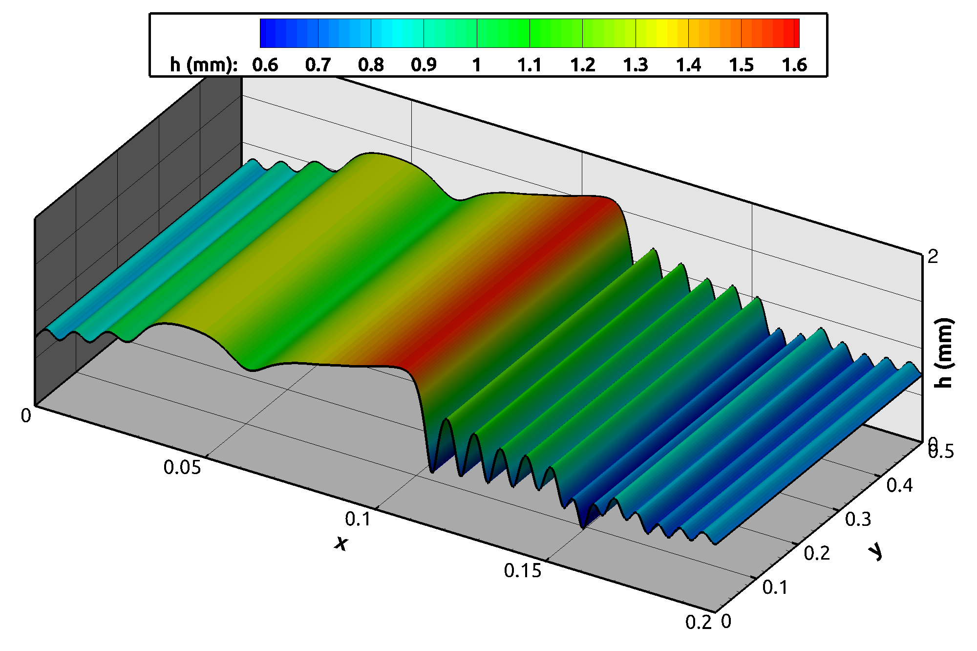
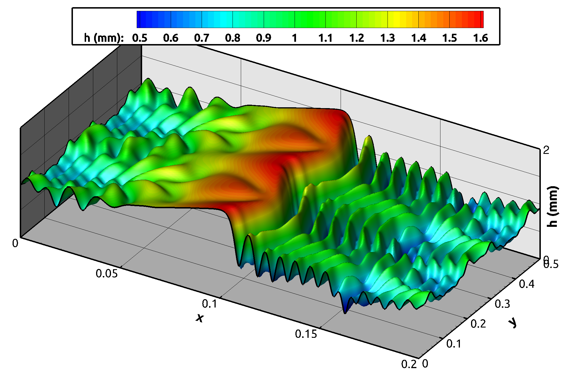
Figure 1: Numerical simulation of a roll-wave in presence of surface tension. On the left: one dimensional roll-wave without transverse perturbations. On the right: a two-dimensional roll-wave

In order to test the robusness of the scheme, we also carried various numerical experiments of a drop falling down a plane in order to deal with wet/dry fronts. For that purpose, we introduced a precusor film with a thickness of $1.0\times 10^{-5}\,mm$.

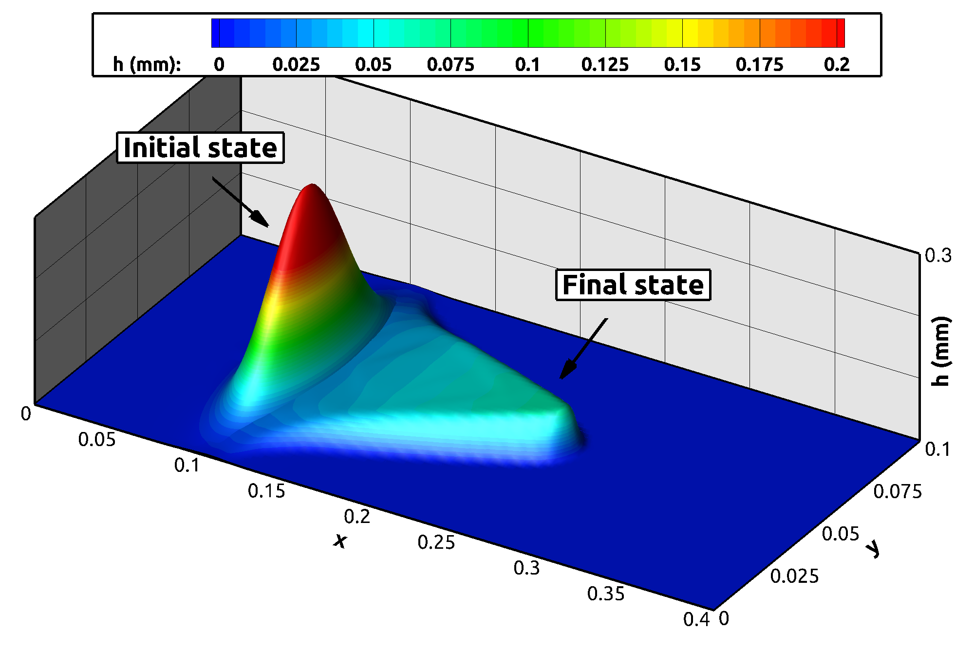
Figure 2: Drop falling down an incline plane ($\theta=60^{o}$) at time $t=0$ and $t=1s$. The fluid density, kinematic viscosity and surface tension are respectively $\rho=1.0\times 10^{3}\,kg.m^{-3}$, $\nu=1.0\times 10^{-6}\,m^{2}.s^{-1}$ and $\sigma=67\times 10^{-3}\,kg.s^{-2}$.

We will deal the problems of considering physical boundary conditions, deriving higher order schemes and considering wet/dry fronts in a forthcoming paper [4]. This will be useful to compute instabilities in moving contact lines.

References

• [1] S. Benzoni-Gavage, R. Danchin, S. Descombes. On the well-posedness for the Euler-Korteweg model in several space dimensions. Indiana University Mathematics Journal, 56, no 4, 1499–1579 (2007).
• [2] D. Bresch, B. Desjardins, C.K. Lin. On some compressible fluid models: Korteweg, lubrication, and shallow water systems. Comm. Partial Differential Equations 28 (2003), no. 3-4, 843–868.
• [3] M. Boutounet, L. Chupin, P. Noble, J.–P. Vila. Shallow water flows for arbitrary topography. Comm. Math. Sci.,6 (2008) no 1, p. 73–90.
• [4] D. Bresch, F. Couderc, P. Noble, J.-P. Vila. Stable schemes for some compressible capillary fluid systems under hyperbolic Courant-Friedrichs-Lewy condition. In preparation.
• [5] D. Bresch, B. Desjardins, E. Zatorska. Two-velocity hydrodynamics in fluid mechanics: Part II Existence of global $\kappa$-entropy solutions to compressible Navier-Stokes systems with degenerate viscosities. To appear J. Math Pures Appl. (2015).
• [6] M.A. Hoefer, M.J. Ablowitz, I. Coddington, E.A. Cornell, P. Engels, V. Schweikhard. Dispersive and classical shock waves in Bose-Einstein condensates and gas dynamics. Physical Review A 74 (2006) no 2, 023623.
• [7] D. Jamet, D. Torres, J.U. Brackbill. On the theory and computation of surface Tension: The elimination of parasitic currents through energy conservation in the second-gradient Method. Journal of Computational Physics 182 (2002) 262–276.
• [8] J. Liu, J.B. Schneider, J.P. Gollub. Three-dimensional instabilities of film flows. Physics of Fluids 7 (1995) no 1, 55–67.
• [9] P. Noble, J.–P. Vila. Stability theory for difference approximations of Euler-Korteweg equations and application to thin film flows. SIAM J. Numer Anal., 52 (2014) no 6, 2770–2791.
• [10] A. Vasseur, C. Yu. Existence of Global Weak Solutions for 3D Degenerate Compressible Navier- Stokes Equations. arXiv:1501.06803, (2015)