Dynamical Schwinger process in a bifrequent electric field of finite duration: survey on amplification

Abstract

The electron-positron pair production due to the dynamical Schwinger process in a slowly oscillating strong electric field is enhanced by the superposition of a rapidly oscillating weaker electric field. A systematic account of the enhancement by the resulting bifrequent field is provided for the residual phase space distribution. The enhancement is explained by a severe reduction of the suppression in both the tunneling and multiphoton regimes.

I Introduction

The developement of new radiation sources offers opportunities for the investigation of fundamental physical processes which hitherto could not be accessed experimentally. In the realm of quantum electrodynamics the Schwinger effect, i.e. the decay of a pure electromagnetic field into electron-positron pairs, is among the challenges which have escaped an experimental verification until now. While pair production via perturbative or even non-linear effects in different forms, mostly including null fields, is well established, the genuinely non-perturbative Schwinger effect schwinger in a static homogenous electric field requires field strengths far beyond current laboratory capabilities. Much hope has been put on optical laser facilities where, in fact, high field strengths can be achieved in the focal spots near to the refraction limit. However, only future developements as, e.g., the pillar-3 part of ELI ELI , could bring the dynamical Schwinger effect (which refers to an alternating electric field) into realistic reach. Here, synchronized counterpropagating laser beams with suitable polarisation can produce regions of an alternating field with a dominating electric component in the vicinity of the antinodes.

In the search for configurations which could enable a verification of the Schwinger effect as a tunneling process the idea has been put forward to enhance the pair creation rate by the assistance of a multi-photon process schutzhold_dynamically_2008 ; dunne_catalysis_2009 . This set-up is denoted as the assisted dynamical Schwinger process. There, one can think of the combination of optical high-intensity laser and XFEL beams, the latter ones representing a fast weak field. In fact, at LCLS such instrumental prepositions are already at our disposal LCLS , and the HIBEF collaboration HIBEF at the European XFEL in Hamburg plans an analogous installation, albeit with different key parameters w.r.t. repetition rates, energies and intensities. Further experimental proposals can be found in alkofer_pair_2001 ; dunne_extreme_2014 ; gonoskov_probing_2013 . Whether such configurations will enable to investigate the Schwinger effect, or a variant thereof, needs to be elucidated.

Given such a motivation, we are going to consider here a model for pair production by a bifrequent, spatially homogenous electric field which acts for a finite time interval. The pair creation process is a non-equilibrium process to be described by a quantum kinetic equation with a strong non-Markovian feature. Such a framework has been employed in various previous analyses, e.g., for the superposition of Sauter pulses orthaber_momentum_2011 ; kohlfurst_optimizing_2013 or periodic fields and Sauter pulses sicking_bachelor_2012 or for two (or more) periodic fields hebenstreit_optimization_2014 ; akal_electron-positron_2014 , and for studying the temporal structure of particle creation blaschke_properties_2013 ; blaschke_dynamical_2014 ; dabrowski_super-adiabatic_2014 . Alternative frameworks make use of WKB-type approximations fey_momentum_2012 , worldline instantons dumlu_complex_2011 ; schneider_dynamically_2014 or lightfront methods hebenstreit_pair_2011 ; ilderton_localisation_2014 . Our goal is to investigate the dynamical Schwinger effect in bifrequent fields systematically over a large region in the parameter space spanned by field strengths and frequencies.

II Residual phase space distribution: Analytical Approximations

The residual phase space distribution $f$ of pairs in a bifrequent electric ${\bm{E}}(t)$ field (frequencies $\nu_{1}$, $\nu_{2}=N\nu_{1}$) which acted for a finite time $t_{\text{f.t.}}$ with constant amplitudes $E_{1}$ and $E_{2}$ is given by (see Appendix)

$$f(p,\varphi,t_{\text{f.t.}})\cong\frac{1}{2}\!\!\sum_{\ell\geq\ell_{\text{min}}}^{\infty}\!\!\left|F_{\ell}\bigl{(}p_{\ell}(\varphi),\varphi\bigr{)}\right|^{2}t_{\text{f.t.}}^{2}S\Bigl{(}\Omega^{\prime}\bigl{(}p_{\ell}(\varphi),\varphi\bigr{)}t_{\text{f.t.}}\bigl{(}p-p_{\ell}(\varphi)\bigr{)}\Bigr{)}\>,$$ (1)

with momentum components perpendicular ($p_{\perp}=p\cos\varphi$) and parallel ($p_{\parallel}=p\sin\varphi$) to ${\bm{E}}$ ($\varphi=-\frac{\pi}{2}\cdots\frac{\pi}{2}$). The function $S(x)=\sin^{2}x/x^{2}$ has a main peak at $x=0$, $S(0)=1$, of width $2\pi$ and an infinite number of side peaks declining as $\sim x^{-2}$. This implies that the phase space distribution (1) for fixed $\varphi$ displays a series of main peaks at $p=p_{\ell}(\varphi)$, see Fig. 1. (Accounting for the $\varphi$ degree of freedom gives rise to ridges over the $p_{\perp}$-$p_{\parallel}$ plane, sometimes called shell structure.) The peak positions $p_{\ell}(\varphi)$ are determined by the resonance condition (cf. otto_lifting_2015 )

$$2\Omega(p_{\ell}(\varphi),\varphi)-\ell\nu_{1}=0\>,$$ (2)

$$\Omega(p_{\perp},p_{\parallel})=\frac{m}{2\pi}\int\limits_{0}^{2\pi}\!\!\mathrm{d}x\left(1+\frac{p_{\perp}^{2}}{m^{2}}+\left(\frac{p_{\parallel}}{m}-\gamma_{1}^{-1}\cos x-\gamma_{2}^{-1}\cos Nx\right)^{2}\right)^{\frac{1}{2}}\!,$$ (3)

where $\gamma_{1,2}=\frac{E_{c}}{E_{1,2}}\frac{\nu_{1,2}}{m}$ are Keldysh parameters with $E_{c}=\frac{e}{m^{2}}$, $-e$ the electron charge and $m$ its mass. Since $\Omega(p_{\ell}(\varphi),\varphi)>m_{*}>m$ with the effective mass $m_{*}=\Omega(p_{\ell}=0)$ (cf. brezin_pair_1970 ; kohlfurst_effective_2014 for the effective mass concept in the single field case), the values of $\ell$ must exceed a certain threshold, $\ell\geq\ell_{\text{min}}=\lceil\frac{2m_{*}}{\nu_{1}}\rceil$, where $\lceil x\rceil$ denotes the smallest integer greater than or equal to $x$.

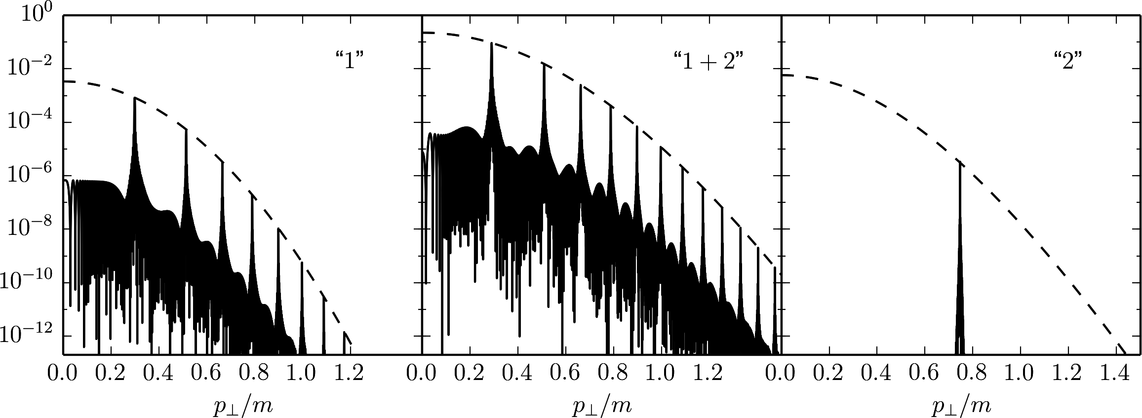
Figure 1: Residual phase space distributions at $p_{\parallel}=0$ (solid curves, from integrating the quantum kinetic equations, e.g. equations (1-7) in otto_lifting_2015 ) for field “1” (left panel, $E_{1}=$0.2$E_{c}$, $\nu_{1}=$0.02$m$, i.e. $\gamma_{1}=$0.1$$), fields “1+2” (middle panel) and field “2” (right panel, $E_{2}=$0.05$E_{c}$, $\nu_{2}=$0.5$m$, i.e. $\gamma_{2}=$10$$). The dashed curves depict the spectral envelope $\frac{2}{9}\nu_{1}^{2}t_{\text{f.t.}}^{2}\mathcal{E}(p_{\perp})$ with $\mathcal{E}$ given by (5). The flat-top duration is determined as in otto_lifting_2015 by $\nu_{1}t_{\text{f.t.}}=2\pi\cdot 50$ and the $C^{\infty}$ ramping (switching-on) and deramping (switching-off) periods are such to cover $5$ oscillations each.

The number of side peaks belonging to $p_{\ell}$ until the next main peak at $p_{\ell+1}$ is about $k=(p_{\ell+1}-p_{\ell})\,\Omega^{\prime}(p_{\ell}(\varphi),\varphi)\,t_{\text{f.t.}}/\pi\gg 1$. This means that the spectrum consists, for sufficiently large $t_{\text{f.t.}}$, of well separated main peaks centered at $p_{\ell}(\varphi)$, with some micro-structures emerging from the superposition of the side peaks encoded in $S$, which are not resolved on the scale displayed in Fig. 1. Due to $\lim\limits_{t_{\text{f.t.}}\rightarrow\infty}S(at_{\text{f.t.}})=2\pi t_{\text{f.t.}}^{-1}\delta(a)$, Eq. (1) asymptotically gets a form derived in popov_resonant_1973 (see also ringwald_pair_2001 ), albeit for a single field and in a low-momentum expansion and for the rate, which is time ($t_{\text{f.t.}}$) independent. We consider here finite values of $t_{\text{f.t.}}$, (i) on the one hand sufficiently large to accomodate at least a few oscillations of both fields “1” and “2” within the flat-top ($t_{\text{f.t.}}$) period of the overall shape function of the potential, and (ii) not too large to avoid the onset of Rabi oscillations akal_electron-positron_2014 which would modify the $t_{\text{f.t.}}$ dependence in (1).

The main peak altitudes are governed by the squared Fourier-coefficients $\left|F_{\ell}\bigl{(}p_{\ell}(\varphi),\varphi\bigr{)}\right|^{2}$ which contain the spectral envelope function $\mathcal{E}(p_{\perp})$. As pointed out in the Appendix, for $p_{\parallel}=0$, they can be approximated by

$$\left|F_{\ell}(p_{\ell},\varphi=0)\right|^{2} \approx\frac{2}{9}\nu_{1}^{2}\mathcal{E}(p_{\ell})\bigl{(}1-(-1)^{\ell}\bigr{)}\>,$$ (4)

$$\mathcal{E}(p_{\perp}) =\mathrm{e}^{-4\frac{m}{\nu_{1}}G(p_{\perp},\gamma_{1},\gamma_{2},N)}\>,$$ (5)

$$G(p_{\perp},\gamma_{1},\gamma_{2},N) =\int\limits_{0}^{x_{0}}\!\!\mathrm{d}x\left(1+\frac{p_{\perp}^{2}}{m^{2}}-\left(\gamma_{1}^{-1}\sinh x+\gamma_{2}^{-1}\sinh Nx\right)^{2}\right)^{\frac{1}{2}}\>,$$ (6)

for the special case $N=4n+1$, $n=0,1,2,\cdots$. The quantity $x_{0}$ is determined by

$$\gamma_{1}^{-1}\sinh x_{0}+\gamma_{2}^{-1}\sinh Nx_{0}=\sqrt{1+p_{\perp}^{2}/m^{2}}\>.$$ (7)

In the single field case ($E_{2}\rightarrow 0$, $\gamma_{2}\rightarrow\infty$), $G$ reduces to

$$G_{1}(p_{\perp},\gamma_{1})=G(\gamma_{2}\rightarrow\infty)=\frac{\pi}{4}\gamma_{1}\left(1+\frac{p_{\perp}^{2}}{m^{2}}\right)g\left(\gamma_{1}\sqrt{1+\frac{p_{\perp}^{2}}{m^{2}}}\right)\>,$$ (8)

where $g(\gamma)={{}_{1}F_{2}}(\frac{1}{2},\frac{1}{2},2,-\gamma^{2})$ is a function already introduced in brezin_pair_1970 , cf. also popov_resonant_1973 . We argue that a handy approximation is provided by

$$G\approx\frac{\pi}{4}\sqrt{1+\frac{p_{\perp}^{2}}{m^{2}}}\,x_{0}$$ (9)

and, analogously,

$$G_{1}\approx\frac{\pi}{4}\sqrt{1+\frac{p_{\perp}^{2}}{m^{2}}}\operatorname*{arsinh}\left(\sqrt{1+\frac{p_{\perp}^{2}}{m^{2}}}\,\gamma_{1}\right)\>.$$ (10)

The former is appropriate for $x_{0}<1$ and the latter for $\sqrt{1+\frac{p_{\perp}^{2}}{m^{2}}}\,\gamma_{1}<10$. The spectral envelopes are displayed in Fig. 1 by dashed curves using (6). Evidently, the envelopes connect the peaks of the fairly rich spectra very well, the details of which are only accessible by integrating the full set of quantum kinetic equations. The approximations (9) and (10) are suitable for conditions as in the left panel of Fig. 1, while (9) gives some semi-quantitative account (within factor of two) for the middle panel.

To understand qualitatively the amplification by a second weak field, as exemplified in Fig. 1 (further examples in otto_lifting_2015 ), one can use the approximation (9) for $p_{\perp}\ll m$ and the first-order iterative solution of (7), $x_{0}=\operatorname*{arsinh}\left(\gamma_{1}-\frac{\gamma_{1}}{\gamma_{2}}\sinh\bigl{[}N\operatorname*{arsinh}\gamma_{1}\bigr{]}\right)$. Supposing $\gamma_{1}\ll 1$ and $N\gamma_{1}\ll 1$ one finds for large $\gamma_{2}$

$$G(\gamma_{1},\gamma_{2},N)\approx G_{1}(\gamma_{1})-\frac{\gamma_{1}^{2}}{\gamma_{2}}N,$$ (11)

i.e. due to the presence of the second field, encoded in $\gamma_{2}$, the modulus of the exponential, $4\frac{m}{\nu_{1}}G_{1}$, becomes diminished by about $4\left(\frac{E_{c}}{E_{1}}\right)^{2}\frac{E_{2}}{E_{c}}$ – interestingly independent of $\nu_{2}$ in the given approximation (which is a special case of the expansion of a multi-scale implicit function). In other words, the spectral envelope of field “1” gets lifted by $\exp\left(4\frac{m}{\nu_{1}}\frac{\gamma_{1}^{2}}{\gamma_{2}}N\right)$ due to the presence of field “2”. In general we stress that, due to the monotonic behavior of the hyperbolic sine functions in (6) and the defining equation (7) for $x_{0}$, one infers $x_{0}(\gamma_{1},\gamma_{2}\rightarrow\infty,N)>x_{0}(\gamma_{1},\gamma_{2},N)>0$ and analogously $G_{1}(\gamma_{1})>G(\gamma_{1},\gamma_{2},N)>0$. Since the negative of $G$ enters the exponential of the envelope function, a dropping of $G$ by the second weak field causes the anticipated amplification. A quantitative consideration is given in the next section.

III Discussion of the Amplification

III.1 Single field case

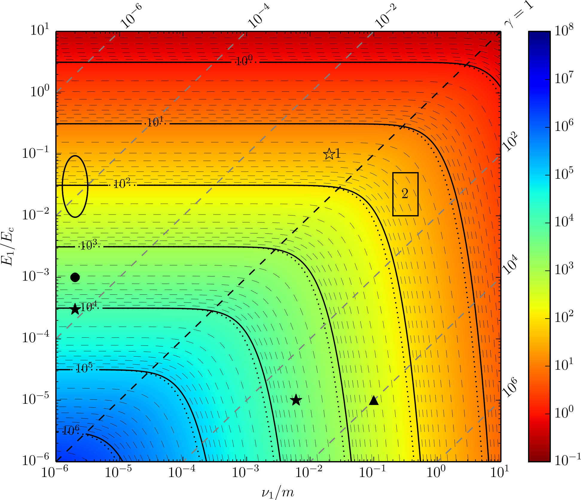
Figure 2: Contour plot of the exponential $4\frac{m}{\nu_{1}}G_{1}=4\frac{m}{\nu_{1}}G(p_{\perp}\ll m,\gamma_{1},\gamma_{2}\rightarrow\infty)$ of the single-field spectral envelope function over the field-frequency ($E_{1}/E_{c}$ vs. $\nu_{1}/m$) plane (solid curves: using (6) for $G$, dotted curves: the approximations (9,10)). Note that the spectral envelope is given by $\frac{2}{9}\nu_{1}^{2}t_{\text{f.t.}}^{2}\mathcal{E}_{1}$ with $\mathcal{E}_{1}=\exp\left(-4\frac{m}{\nu_{1}}G_{1}\right)$. Lines (dashed) of constant Keldysh parameters are displayed too. Parameters from table 1 in ringwald_pair_2001 are depicted by stars, while the bullet is for ELI-NP eli-np ; the ellipse is a former perspective of ELI used, e.g., in schutzhold_dynamically_2008 ; dunne_catalysis_2009 . The triangle is for MaRIE at LANL carlsten_marie_2011 . Point 1 and the square 2 depict parameters considered in otto_lifting_2015 , where the validity of Eqs. (1)-(6) can be checked by numerical integration of the quantum kinetic equations, as is also exemplified in Fig. 1. Light grey dashed contour curves are for $2,\cdots,9$ between the solid decade contour curves.

In the following we consider $\mathcal{E}=\exp\left(-4\frac{m}{\nu_{1}}G(p_{\perp},\gamma_{1},\gamma_{2},N)\right)$ as the essential part of the spectral envelope of the phase space distribution. The benchmark for the following discussion is the reference distribution for one periodic field, i.e. $\gamma_{2}\rightarrow\infty$ as realized by $E_{2}\rightarrow 0$. The exponential $4\frac{m}{\nu_{1}}G_{1}$ of the spectral envelope function $\mathcal{E}_{1}$ is displayed in Fig. 2. The region $\gamma_{1}<1$ is often termed adiabatic (tunneling) region where the residual pair density is independent of frequency, while $\gamma_{1}>1$ is the anti-adiabatic (multi-photon) region which is weakly dependent on the field strength. Focusing on low-momentum particles, $p_{\perp}/m\ll 1$, the spectral envelope in the adiabatic region behaves as $\exp\bigl{(}-\pi(E_{c}/E_{1})\bigr{)}$, while in the anti-adiabatic region it behaves like $\exp(-4\frac{m}{\nu_{1}}\log 4\gamma_{1}+4\frac{m}{\nu_{1}})$ in leading order based on (9). The contours (solid curves) in Fig. 2 are based on (6); they differ marginally on the approximate estimates (9) (dotted curves). Figure 2 provides a quantitative description of the landscape of the dynamical Schwinger effect, first qualitatively discussed in blaschke_properties_2013 . Note the huge variation over the displayed parameter range by recollecting that the residual phase density at $p_{\parallel}=0$ is bounded from above by $\frac{2}{9}\nu_{1}^{2}t_{\text{f.t.}}^{2}\mathcal{E}_{1}$ with $\mathcal{E}_{1}=\exp\left(-4\frac{m}{\nu_{1}}G_{1}\right)$, i.e. in the blue region one meets a very strong suppression of the pair density, guaranteeing a long lifetime of the vacuum. Only the red region above the $\gamma_{1}=1$ line seems to allow for verifying experimentally Schwinger’s tunneling process in one oscillating field. As pointed out in otto_lifting_2015 (see also akal_electron-positron_2014 and further references therein), the impact of a second field can significantly reduce the strong suppression due to large values of $4\frac{m}{\nu_{1}}G$, i.e., it results in an amplification effect, as mentioned above.

III.2 Two field case: Amplification

The key for an interpretation of the amplification effect by an assisting field ($\nu_{2}$, $E_{2}$) is the approximation (9) for $p_{\perp}\ll m$: Since $x_{0}(\gamma_{1},\gamma_{2},N)<x_{0}(\gamma_{1},\gamma_{2}\rightarrow\infty)$, the spectral envelope function $\mathcal{E}_{1}=\exp\left(-4\frac{m}{\nu_{1}}G_{1}\right)$ is lifted by the amount $\mathcal{E}_{1+2}/\mathcal{E}_{1}=\exp\bigl{(}4\frac{m}{\nu_{1}}\bigl{[}-G(\gamma_{1},\gamma_{2},N)+G_{1}(\gamma_{1})\bigr{]}\bigr{)}\approx\exp\bigl{(}\pi\frac{m}{\nu_{1}}\bigl{[}-x_{0}(\gamma_{1},\gamma_{2},N)+x_{0}(\gamma_{1},\gamma_{2}\rightarrow\infty)\bigr{]}\bigr{)}$, where $\mathcal{E}_{1+2}=\exp\left(-4\frac{m}{\nu_{1}}G(\gamma_{1},\gamma_{2},N)\right)$. Due to the usually considered range of values $\frac{m}{\nu_{1}}$, even a moderate reduction of $G$ (or $x_{0}$) due to the assisting field, e.g. by $\mathcal{O}(50\%)$, leads to a huge reduction of the suppression in the subcritical region $E_{1}/E_{c}\ll 1$ and $\nu_{1}/m\ll 1$ steered either by $\frac{m}{\nu_{1}}\gamma_{1}=E_{c}/E_{1}$ in the adiabatic region or by $\frac{m}{\nu_{1}}\log\gamma_{1}$ in the anti-adiabatic region.

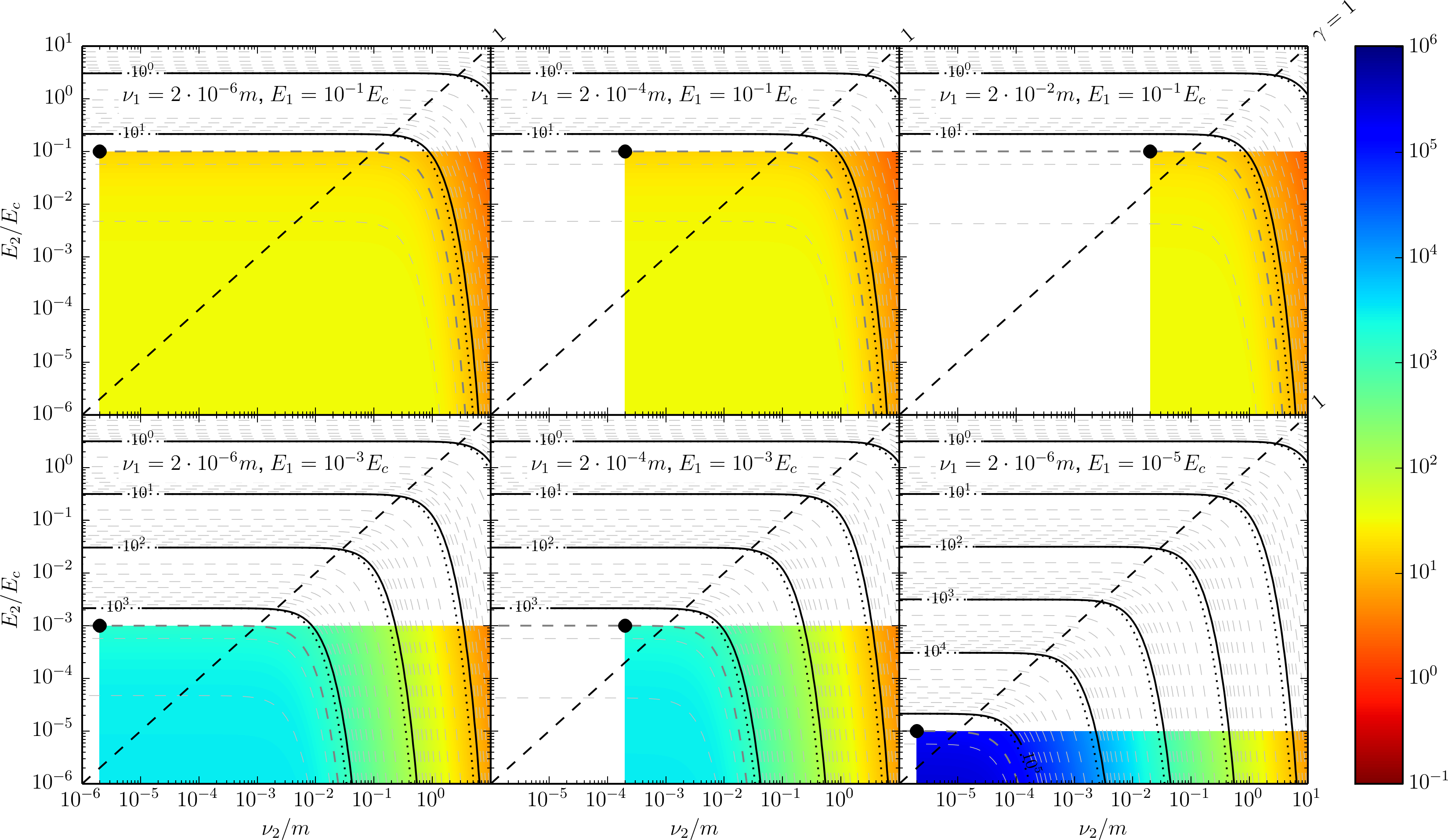
Figure 3: Contour plots of the exponential $4\frac{m}{\nu_{1}}G(p_{\perp}\ll m,\gamma_{1},\gamma_{2},N)$ for six given fields $\nu_{1}$, $E_{1}$ in the adiabatic region (positions depicted by the bullets, which are the loci of field doubling) over the field-frequency ($E_{2}/E_{c}$ vs. $\nu_{2}/m$) plane, i.e. actually $4\frac{m}{\nu_{1}}G(p_{\perp}\ll m,\nu_{1},E_{1},\nu_{2},E_{2})$. Despite of the displayed smooth distribution, our results are strictly valid only for $E_{2}<E_{1}$ and $\nu_{2}=(4n+1)\nu_{1}$, $n=0,1,2\cdots$. Light grey dashed contour curves are for $2,\cdots,9$ between the solid decade contour curves. The heavy grey dashed curves are constructed to go through the bullets. An amplification beyond the field doubling occurs in the colored regions right to the heavy grey dashed curves.

A few examples are exhibited in Fig. 3, where we show the exponential $4\frac{m}{\nu_{1}}G(p_{\perp}\ll m,\gamma_{1},\gamma_{2},N)$, entering the spectral envelope $\frac{2}{9}\nu_{1}^{2}t_{\text{f.t.}}^{2}\mathcal{E}_{1+2}$, for a few selected fields $E_{1}$, $\nu_{1}$ over the $E_{2}$-$\nu_{2}$ plane. As reference one has to take the spectral envelope function from Fig. 2. The value of the envelope exponential is trivially reduced by $50\%$ in the points $E_{2}=E_{1}$ and $\nu_{2}=\nu_{1}$ (marked by symbols in Fig. 2), i.e. simply doubling the field strength. This is the lowest order of the multi-field configurations considered in narozhny_pair_2004 . Further amplification occurs for enlarging $\nu_{2}$, as signalled by a reduction of $4\frac{m}{\nu_{1}}G$. That is, the amplification beyond the field doubling happens in the region right to the contour curve (heavy grey dashed) going through the reference point (bullet) $E_{2}=E_{1}$, $\nu_{2}=\nu_{1}$. The single field result is recovered by inspection of $E_{2}\rightarrow 0$, i.e. going down from the reference point at $\nu_{1}$, $E_{1}$. Note that our amplification estimate by formula (4) requires $E_{2}<E_{1}$ and $\nu_{2}=N\nu_{1}$ with $N=4n+1$, $n=0,1,2\cdots$, that is our result holds true actually only at discrete values of $\nu_{2}$.

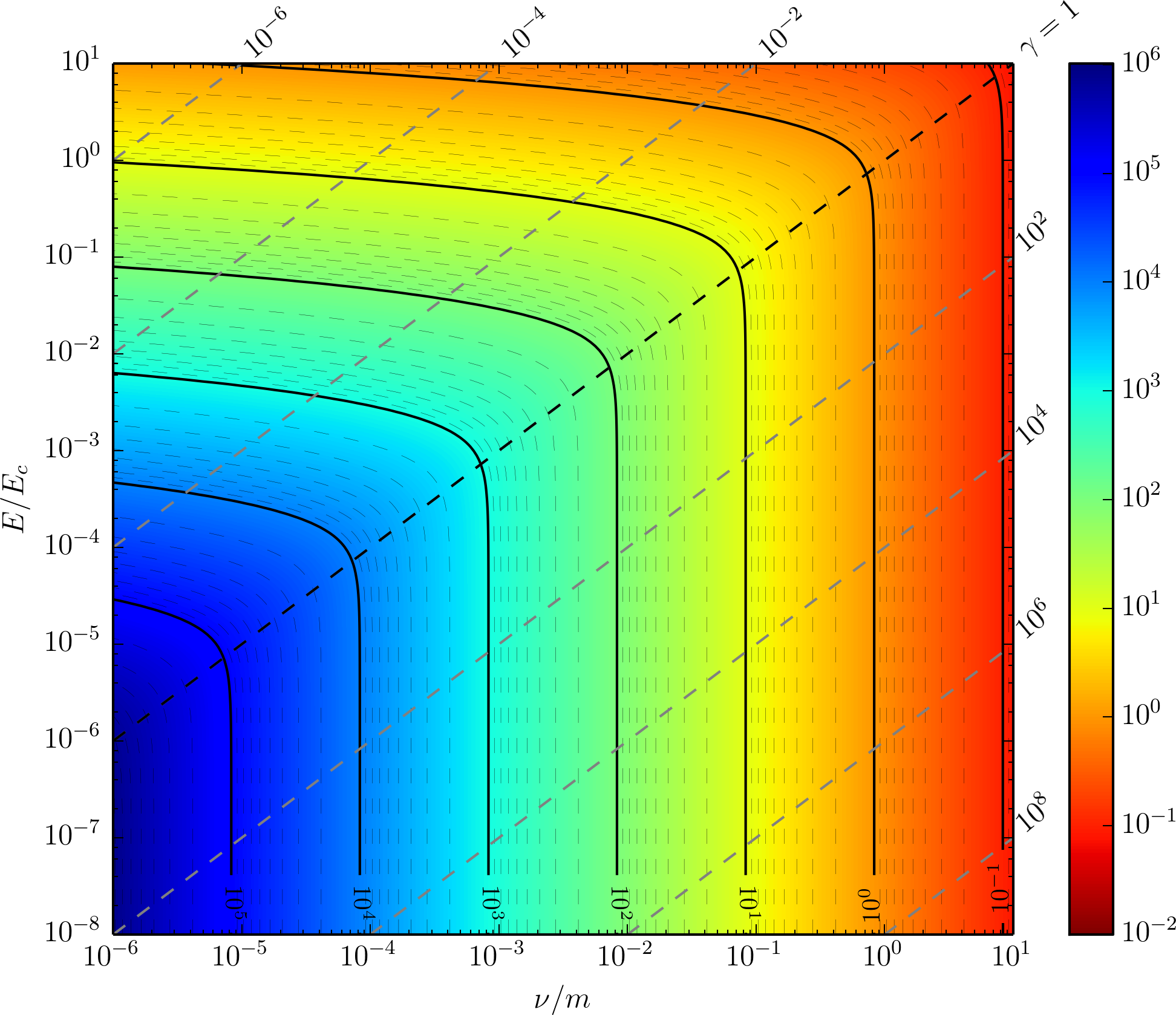
Figure 4: Contour plot of the number of main peaks in the inverval $p_{\perp}=0\cdots m$ at $p_{\parallel}=0$ for the action of one field characterized by $\nu$ and $E$. Light grey dashed contour curves are for $2,\cdots,9$ between the solid decade contour curves. Dashed lines depict constant Keldysh parameters.

The net outcome points to the importance of the frequency $\nu_{2}$, while variations of $E_{2}$ are subleading. To achieve amplifications which overcome the strong suppression in the tunneling regime one has to employ frequencies $\nu_{2}$ near or above critical range $\nu\gtrsim m$, where essentially the multi-photon process sets the scale, i.e. one has to compare the phase space population with the one for the $\nu_{2}$, $E_{2}$ field alone. This is accomplished by inspecting Fig. 2 for the exponential of the spectral envelope function and by correcting the pre-exponential factor in (4) by $\nu_{1}\rightarrow\nu_{2}$. As shown in otto_lifting_2015 for selected examples (see also Fig. 1), the action of the field ($\nu_{2}$, $E_{2}$) lifts the phase space distribution emerging from ($\nu_{1}$, $E_{1}$) alone above the one of ($\nu_{2}$, $E_{2}$) alone. A decisive difference is in the density of states (peaks) in the $p_{\perp}(p_{\parallel})$ distributions: The number of peaks within $p_{\perp}=0\cdots m$ is given by $\frac{2}{\nu_{1}}\bigl{[}\Omega(p=m,\varphi=0,\gamma_{1},\gamma_{2},N)-\Omega(p=0,\varphi=0,\gamma_{1},\gamma_{2},N)\bigr{]}$, which can be much larger for the field ($\nu_{1}$, $E_{1}$) alone than the field ($\nu_{2}$, $E_{2}$) alone, depending on the locus in the $\nu$-$E$ plane, see Fig. 4.

IV Discussion

The goal of our paper is to provide a qualitative understanding for the amplification of the pair creation rate in a periodic electric field under the resonant assistance of a second faster and weaker electric field. In the quantum kinetic approach, such an investigation would require scans of the four-dimensional parameter space $E_{1,2}$, $\nu_{1,2}$ for a dense set of points in the two-dimensional $p_{\perp}$-$p_{\parallel}$ phase space. In addition, the impact of the temporal structure (details of switching on/off and duration of the flat top time span) should be considered. To avoid such a cumbersome wealth of information we refrain from considering the harsh landscape of the phase space distribution by analysing only its spectral envelope instead. As a consequence, we do not need to consider the details of the peak (ridge) positions, which are modified by the assistance field. We also rely on the previous observation otto_lifting_2015 concerning the dependence of the residual phase space distribution on the time structure. This in turn is based on a harmonic analysis in the low-density approximation otto_lifting_2015 .

Under these conditions, the amplification, observed in several previous investigations which are restricted to small patches in the parameter space, can be explained as a reduction of the huge suppression provided by $\exp(-\pi(E_{c}/E_{1})x_{0})$ in the adiabatic or by $\exp(-4(m/\nu)x_{0})$ in the anti-adiabatic regimes: by the assistance field, the quantity $x_{0}$ (the zero of a simple function) becomes smaller. Applying these findings to typical parameters which represent the optical laser–XFEL combination according to ringwald_pair_2001 we find a promising perspective for laser intensities only significantly above the present ELI-NP plan eli-np . More promising is the laser-$\gamma$ beam combination, as already pointed out in schutzhold_dynamically_2008 ; dunne_catalysis_2009 for ultra-intense laser beams, but we see also a good discovery potential for ELI-NP eli-np and even multi-PW lasers. The potentially dangerous $\gamma$ conversion processes might be rejected by the phase space distribution of the residual pairs: The amplified tunneling production displays the distinct peak (ridge) structure dictated by the frequency $\nu_{1}$.

To arrive at such a simple picture we made two restrictions: (i) $N=4n+1$, $n=0,1,2,\cdots$ was selected since the main pole in the complex time plane is then shifted in purely imaginary direction towards the real axis under the action of the assistance field (see Appendix), thus allowing for an easy access to the spectral envelope function and (ii) $p_{\parallel}=0$ was chosen as it was shown in otto_lifting_2015 to provide a proper orientation. The avenues for next generalizations are obvious: extensions to arbitrary integer $N$ (and further also real $N$ which go beyond the resonant type patterns) as well as further poles and estimates of the phase space-integrated residual distribution to arrive at a density. Still, the model is fairly simple and needs further considerations of important effects, such as spatial inhomogenities which are, for example, elaborated in dunne_worldline_2005 ; ruf_pair_2009 ; schneider_dynamically_2014 .

V Summary

In summary we provide a comprehensive tool to access the amplification of the dynamical Schwinger process by a resonantly assisting second field, both acting for a finite duration. A promising perspective is seen in the combination of ultra-intense optical laser beams with $\gamma$ beams, while the optical laser-XFEL combination also allows for huge amplification effects, however, probably not sufficient to enable an experimental verification.

Appendix: Derivation of Eqs. (1)-(6)

In the low-density approximation of the quantum kinetic equation schmidt_quantum_1998 ; mamayev_mostepanenko , the electron-positron pair density $f$ is given by $f({\bm{p}},t)=\frac{1}{2}\left|I({\bm{p}},t)\right|^{2}$ with

$$I({\bm{p}},t) =\int\limits_{0}^{t}\!\frac{eE(t^{\prime}){\epsilon_{\perp}}}{\omega({\bm{p}},t^{\prime})^{2}}\mathrm{e}^{2i\Theta({\bm{p}},t^{\prime})}\mathrm{d}t^{\prime}\>,$$ (12)

where we introduced ${\epsilon_{\perp}}=\sqrt{m^{2}+p_{\perp}^{2}}$, $\omega({\bm{p}},t)=\sqrt{m^{2}+p_{\perp}^{2}+\bigl{(}p_{\parallel}-eA(t)\bigr{)}^{2}}$, $\Theta({\bm{p}},t)=\int\limits_{0}^{t}\!\mathrm{d}t^{\prime}\omega({\bm{p}},t^{\prime})$. The vector potential $A(t)$ and hence the electric field $E(t)=-\dot{A}(t)$ are assumed to be periodic in time, e.g. $A=(E_{1}/\nu_{1})\cos(\nu_{1}t)+(E_{2}/(N\nu_{1}))\cos(N\nu_{1}t)$ over a finite time span $t_{\text{f.t.}}$, much longer than the switching-on/off intervals. Accordingly one can split $\Theta$ in a linearly growing and a periodic part, $\Theta({\bm{p}},t)=\Omega({\bm{p}})t+P({\bm{p}},t)$, to arrive at $I({\bm{p}},t)=\int\limits_{0}^{t}\!\!\mathrm{d}t^{\prime}F({\bm{p}},t^{\prime})\mathrm{e}^{2i\Omega({\bm{p}})t^{\prime}}$ with $F({\bm{p}},t)=\frac{eE(t){\epsilon_{\perp}}}{\omega({\bm{p}},t)^{2}}\mathrm{e}^{2iP({\bm{p}},t)}$. The function $F$ is time periodic and is decomposed into Fourier modes, $F({\bm{p}},t)=\sum_{\ell}F_{\ell}({\bm{p}})\mathrm{e}^{-i\ell\nu t}$, so that $I$ turns into

$$I({\bm{p}},t)=\sum_{\ell}iF_{\ell}({\bm{p}})\frac{\mathrm{e}^{-i\bigl{(}\ell\nu-2\Omega({\bm{p}})\bigr{)}t}-1}{\ell\nu-2\Omega({\bm{p}})}\>.$$ (13)

The quantity $I$ becomes large whenever $2\Omega({\bm{p}})-\ell\nu$ is small, yielding (2) and (3). Employing polar coordinates one defines the ridge radius $p_{\ell}(\varphi)$ by $2\Omega\bigl{(}p_{\ell}(\varphi),\varphi\bigr{)}-\ell\nu=0$. Since $\Omega(p,\varphi)$ as a function of $p$ is strictly monotonous, this resonance equation has solutions only for $\ell\geq\ell_{\text{min}}=\left\lceil\frac{2\Omega(0,\varphi)}{\nu}\right\rceil$. Expanding every summand in $I$ around its corresponding peak position at $p_{\ell}$ to first order, and keeping $F_{\ell}$ fixed, we arrive at

$$I({\bm{p}},t)=\sum_{\ell=\ell_{\text{min}}}iF_{\ell}\bigl{(}p_{\ell}(\varphi),\varphi\bigr{)}\frac{\exp\left[2i\Omega^{\prime}\bigl{(}p_{\ell}(\varphi),\varphi\bigr{)}\bigl{(}p-p_{\ell}(\varphi)\bigr{)}t\right]-1}{2i\Omega^{\prime}\bigl{(}p_{\ell}(\varphi),\varphi\bigr{)}\bigl{(}p-p_{\ell}(\varphi)\bigr{)}}\>;$$ (14)

terms with $\ell<\ell_{\text{min}}$ do not contribute and are thus dropped. The prime denotes the derivative w.r.t. $p$, i.e. $\Omega^{\prime}(p,\varphi)=\partial\Omega(p,\varphi)/\partial p$. To arrive at $f$ one must take the squared modulus of (14). Terms mixing different $\ell$s in this square will go to zero upon switching off, as one can argue from a slowly varying envelope approximation. So only the non-mixing terms survive for $t>t_{\text{f.t.}}$, yielding in particular the $\sin^{2}x/x^{2}$ part of Eq. (1), which contains ridge positions and ridge widths as anticipated in otto_lifting_2015 . For larger times $t_{\text{f.t.}}$ and small momenta, the Popov formula popov_resonant_1973 ; ringwald_pair_2001 ) is recovered for the special case $E_{2}=0$.

Figure 5: The integration path $\Gamma_{1}$ from $-T/2$ to $+T/2$ along the real axis in (15) is substituted by the sequence $\Gamma_{2}+\Gamma_{3}+\Gamma_{4}+\Gamma_{5}$ in the upper half of the complex $t$ plane. Dots depict the zeros of $\omega(t)^{2}$, where branch cuts (dashed lines) emerge.

What remains is a formula for the Fourier coefficients $F_{\ell}$, which determine the ridge heights. This can be achieved by deforming the integration contour in the complex time plane and using the method of steepest descent, similar to brezin_pair_1970 . For the single field case, the Fourier coefficients are given by

$$F_{\ell}\bigl{(}p_{\ell}(\varphi),\varphi\bigl{)}=\frac{1}{T}\int\limits_{-T/2}^{T/2}\!\frac{eE(t){\epsilon_{\perp}}}{\omega\bigl{(}p_{\ell}(\varphi),\varphi,t\bigl{)}^{2}}\mathrm{e}^{2i\Theta(p_{\ell}(\varphi),\varphi,t)}\mathrm{d}t\>.$$ (15)

The function $\omega(t)^{2}$ has four zeros of first order in the strip $-T/2<\operatorname{Re}t<T/2$ in the complex time plane at $t_{0}$, $t_{0}^{*}$, $-t_{0}$ and $-t_{0}^{*}$. We deform the integration contour to the sequence $\Gamma_{2}+\Gamma_{3}+\Gamma_{4}+\Gamma_{5}$ shown in Fig. 5. The contributions from $\Gamma_{2}$ and $\Gamma_{5}$ cancel due to the periodicity of the integrand. The contribution from $\Gamma_{4}$ is the negative of the complex conjugate of that from $\Gamma_{3}$, in symbolic notation $\int_{\Gamma_{1}}=-\int_{\Gamma_{3}}-\int_{\Gamma_{4}}=-2i\operatorname{Im}\int_{\Gamma_{3}}$. To evaluate the latter integral approximately, we note that the exponent in the integrand is stationary at $t_{0}$. One chooses $\Gamma_{3}$ such that $\operatorname{Im}\Theta$ grows rapidly on $\Gamma_{3}$ away from $t_{0}$, so that $\mathrm{e}^{2i\operatorname{Im}\Theta}$ quickly goes to zero (method of steepest descent). Then only contributions to the integral close to $t_{0}$ matter, thus enabling an expansion $\omega(t)^{2}=2i{\epsilon_{\perp}}eE(t_{0})(t-t_{0})+\mathcal{O}\bigl{(}(t-t_{0})^{2}\bigr{)}$ yielding (we suppress the momentum arguments)

$$\frac{eE(t){\epsilon_{\perp}}}{\omega(t)^{2}}=\frac{1}{2i}\frac{1}{t-t_{0}}+\mathcal{O}(1)\>.$$ (16)

The expansion of the exponent uses $\Theta(t)=\int_{0}^{t}\!\mathrm{d}t^{\prime}\omega(t^{\prime})=\int_{0}^{t_{0}}\!\mathrm{d}t^{\prime}\omega(t^{\prime})+\int_{t_{0}}^{t}\!\mathrm{d}t^{\prime}\omega(t^{\prime})=\Theta(t_{0})+\int_{t_{0}}^{t}\!\mathrm{d}t^{\prime}\sqrt{2eE(t_{0}){\epsilon_{\perp}}}\sqrt{i(t^{\prime}-t_{0})}+\mathcal{O}\bigl{(}(t-t_{0})^{\frac{5}{2}}\bigr{)}$ with the result

$$\Theta(t)=\Theta(t_{0})-\frac{2}{3}i\sqrt{2eE(t_{0}){\epsilon_{\perp}}}\bigl{(}i(t-t_{0})\bigr{)}^{\frac{3}{2}}+\mathcal{O}\bigl{(}(t-t_{0})^{\frac{5}{2}}\bigr{)}\>.$$ (17)

Inserting (16) and (17) into (15) yields our desired result

$$F_{\ell}=-\frac{1}{T}i\operatorname{Im}\int\limits_{\Gamma_{3}}\!\!\mathrm{d}t\,\mathrm{e}^{2i\Theta(t_{0})}\frac{\mathrm{e}^{\frac{4}{3}\sqrt{2eE(t_{0}){\epsilon_{\perp}}}(i(t-t_{0}))^{\frac{3}{2}}}}{i(t-t_{0})}=\frac{4\pi i}{3T}\operatorname{Im}\mathrm{e}^{2i\Theta(t_{0})}=\frac{2}{3}i\nu\operatorname{Im}\mathrm{e}^{2i\Theta(t_{0})}\>.$$ (18)

To generalize to two fields we need to sum over all complex zeros $t_{i}$ of $\omega^{2}$ with $0\leq\operatorname{Re}t_{i}<T/2$, $T=2\pi/\nu_{1}$, and $\operatorname{Im}t_{i}>0$, leading to

Figure 6: The distribution of the zeros of $\omega^{2}$ in the upper half plane for field “1+2” (red squares) for the example of $N=25$. The two zeros for field “1” are shown as black dots, which get shifted down (arrows) upon the impact of field “2”.

$$F_{\ell}\bigl{(}p_{\ell}(\varphi),\varphi\bigr{)}\approx\frac{2}{3}i\nu\sum_{i}\operatorname{Im}\mathrm{e}^{2i\Theta(p_{\ell}(\varphi),\varphi,t_{i})}\>.$$ (19)

It is instructive to take $\varphi=0$, that is we consider the phase space distribution for $p_{\parallel}=0$. For the case $N=4n+1$, integer $n$, a sequence of $N+1$ zeros appears at $\operatorname{Im}t>0$, $-T/2<\operatorname{Re}t<T/2$ (see Fig. 6, red squares). In particular, the zeros at $\pm T/4+ix_{0}/\nu_{1}$ get shifted down, since $x_{0}$ is smaller in the two-field case than in the single-field case. The sum in (19) is dominated by the contribution with the smallest imaginary part, which is the zero $t_{0}=T/4+ix_{0}/\nu_{1}$. Keeping this leading term and using furthermore $\Theta(T)=4\Theta(T/4)$ yields

$$\Theta(t_{0})=\frac{\ell\pi}{4}+i\frac{m}{\nu}\int\limits_{0}^{x_{0}}\!\!\mathrm{d}x\sqrt{1+\frac{p_{\perp}^{2}}{m^{2}}-\left(\frac{1}{\gamma_{1}}\sinh x+\frac{1}{\gamma_{2}}\sinh Nx\right)^{2}}\>,$$ (20)

finally leading to (4) and (6). The amplification effect by a second assistance field is thus rooted in a shift of the leading-order pole towards the real axis in the complex $t$ plane. The condition $E_{2}\leq E_{1}$ ensures the pattern exhibited in Fig. 6 and $N=4n+1$ is specific for the shift of the single field zeros (black dots in Fig. 6) parallel to the imaginary $t$ axis.

References

- (1) J. Schwinger, Phys. Rev. 82 (1951) 664.
- (2) European Extreme Light Infrastructure (ELI), www.eli-laser.eu.
- (3) R. Schützhold et al., Phys. Rev. Lett. 101 (2008) 130404.
- (4) G. V. Dunne et al., Phys. Rev. D 80 (2009) 111301.
- (5) Linac Coherent Light Source, lcls.slac.stanford.edu.
- (6) The HIBEF project, www.hzdr.de/hgfbeamline.
- (7) R. Alkofer et al., Phys. Rev. Lett. 87 (2001) 193902.
- (8) G. V. Dunne, Eur. Phys. J. Spec. Top. 223 (2014) 1055.
- (9) A. Gonoskov et al., Phys. Rev. Lett. 111 (2013) 060404.
- (10) M. Orthaber et al., Phys. Lett. B 698 (2011) 80.
- (11) C. Kohlfürst et al., Phys. Rev. D 88 (2013) 045028.
- (12) J. Sicking, Pulsformabhängigkeit im dynamisch verstärkten Sauter-Schwinger-Effekt, Bachelor thesis, Universität Duisburg-Essen (2012).
- (13) F. Hebenstreit and F. Fillion-Gourdeau, Phys. Lett. B 739 (2014) 189.
- (14) I. Akal et al., Phys. Rev. D 90 (2014) 113004.
- (15) D. B. Blaschke et al., Phys. Rev. D 88 (2013) 045017.
- (16) D. B. Blaschke et al., arXiv:1412.6372 (2014).
- (17) R. Dabrowski and G. V. Dunne, arXiv:1405.0302 (2014).
- (18) C. Fey and R. Schützhold, Phys. Rev. D 85 (2012) 025004.
- (19) C. K. Dumlu and G. V. Dunne, Physical Review D 84 (2011) 125023.
- (20) C. Schneider and R. Schützhold, arXiv:1407.3584 (2014).
- (21) F. Hebenstreit et al., Phys. Rev. D 84 (2011) 125022.
- (22) A. Ilderton, J. High Energy Phys. 2014 (2014) 166.
- (23) A. Otto et al., Phys. Lett. B 740 (2015) 335.
- (24) E. Brezin and C. Itzykson, Phys. Rev. D 2 (1970) 1191.
- (25) C. Kohlfürst et al., Phys. Rev. Lett. 112 (2014) 050402.
- (26) V. S. Popov, JETP Lett. 18 (1973) 255.
- (27) A. Ringwald, Phys. Lett. B 510 (2001) 107.
- (28) ELI Nuclear Physics (ELI-NP), www.eli-np.ro.
- (29) B. E. Carlsten et al., in Proc. 2011 Part. Accel. Conf, page 799 (2011).
- (30) N. B. Narozhny et al., Phys. Lett. A 330 (2004) 1.
- (31) G. V. Dunne and C. Schubert, Phys. Rev. D 72 (2005) 105004.
- (32) M. Ruf et al., Phys. Rev. Lett. 102 (2009) 080402.
- (33) S. M. Schmidt et al., Int. J. Mod. Phys. E 7 (1998) 709.
- (34) V. M. Mostepanenko et al., Vacuum Quantum Effects in Strong Fields, Friedmann Laboratory Publishing Ltd., St. Petersburg (1994).