Two-particle irreducible effective actions versus resummation: analytic properties and self-consistency

Abstract

Approximations based on two-particle irreducible (2PI) effective actions (also known as $\Phi$-derivable, Cornwall-Jackiw-Tomboulis or Luttinger-Ward functionals depending on context) have been widely used in condensed matter and non-equilibrium quantum/statistical field theory because this formalism gives a robust, self-consistent, non-perturbative and systematically improvable approach which avoids problems with secular time evolution. The strengths of 2PI approximations are often described in terms of a selective resummation of Feynman diagrams to infinite order. However, the Feynman diagram series is asymptotic and summation is at best a dangerous procedure. Here we show that, at least in the context of a toy model where exact results are available, the true strength of 2PI approximations derives from their self-consistency rather than any resummation. This self-consistency allows truncated 2PI approximations to capture the branch points of physical amplitudes where adjustments of coupling constants can trigger an instability of the vacuum. This, in effect, turns Dyson’s argument for the failure of perturbation theory on its head. As a result we find that 2PI approximations perform better than Padé approximation and are competitive with Borel-Padé resummation. Finally, we introduce a hybrid 2PI-Padé method.

1 Introduction

Two-particle irreducible (2PI) effective actions and approximation schemes based on them are often touted as useful techniques when it is necessary to go beyond the standard perturbative field theory, with applications to thermal and non-equilibrium plasmas/fluids, strongly coupled quantum field theories and systems dominated by many-body collective effects. The technique was originally developed by Lee and Yang [1], Luttinger and Ward [2], Baym [3] and others in the context of many-body theory, then extended by Cornwall, Jackiw and Tomboulis [4] to relativistic field theory where it found its natural formulation in terms of functional integrals. Since then a broad literature has developed surrounding 2PI effective actions and their generalizations (see [5] for a good introductory review).

Approximations based on 2PI effective actions are often justified as a selective re-summation of perturbation theory (some recent examples: [6, 7, 8]; interestingly though, this point of view is not found in the Cornwall, Jackiw and Tomboulis paper [4]), however they are not really a summation method in the same sense as, for example, Borel summation. Rather, this interpretation comes in a rather roundabout way. First, a set of self-consistent equations of motion is derived for the mean field $\varphi=\left\langle\phi\right\rangle$ and connected correlation function $\Delta=\left\langle\phi^{2}\right\rangle-\left\langle\phi\right\rangle^{2}$, starting directly from the non-perturbative definition of the theory through the path integral. Only after formally solving the equations of motion by repeatedly iterating them does one obtain the usual perturbative expansion for these quantities or, if the equations of motion are truncated, a selective re-summation of perturbation theory appears.

In this work we attempt to clarify the connection between 2PI approximations, traditional perturbation theory and re-summation methods with a special emphasis on what analytic features of the 2PI formalism allow improved approximations to be obtained in the presence of a divergent Feynman diagram series. Unfortunately robust comparisons are difficult because the large order behaviour of perturbation theory is known, at best, in a sketchy form for most field theories of interest. To that end we restrict attention to a genuinely trivial model “field theory” in zero spacetime dimensions (i.e. probability theory) for which exact results are easily obtainable and all complications due to renormalization etc. disappear. This model nevertheless accurately represents the typical combinatoric structure of large order perturbation theory, at least in those cases where the behaviour is known in more interesting field theories. We also introduce a “spectral function” representation of the Green function (similar to the one first introduced by Bender and Wu [9, 10]) to capture the non-analyticity of the solutions in the various methods.

The existence of the spectral representation is connected to the branch cut of physical amplitudes on the negative coupling ($\lambda$) axis. This branch cut is due to the non-existence of the theory at negative couplings: the path integral diverges due to a potential unbounded from below. In a higher dimensional field theory this has a simple physical interpretation: the vacuum is unstable and, after tunneling through a barrier, the system rolls down the potential [11]. For weak coupling the semi-classical approximation is valid and the tunneling is exponentially suppressed, giving an imaginary contribution $\sim\exp\left(-1/\lambda\right)$ to the vacuum persistence amplitude which is inherited by the Green function. This exponential behaviour can be seen in the spectral function we obtain.

Dyson [12] argued that a very similar phenomenon occurs in quantum electrodynamics (QED). We briefly reiterate this argument. In QED physical observables are calculated in a perturbation series of the form $F\left(e^{2}\right)=a_{0}+a_{2}e^{2}+a_{4}e^{4}+\cdots$ where $e\sim 0.3$ is the charge of the electron. Now if one imagines a world where $e^{2}<0$, i.e. like charges attract, it is easy to see that the ordinary vacuum is unstable to the production of many electron-positron pairs which separate into clouds of like-charged particles. At weak coupling there is a large tunneling barrier to overcome because one must pay for the rest mass of the pairs and separate them far enough for the wrong-sign Coulomb potential to compensate. Thus there is a finite but exponentially suppressed rate of vacuum decay. A Taylor series expansion in $e^{2}$ cannot capture this non-analyticity so the perturbation series must be divergent.

Similarly, the perturbation series in $\lambda$ diverges for the toy model considered here. Padé approximants are more effective because they can develop isolated poles in the complex $\lambda$ plane, however they struggle to capture the strong coupling behaviour at any fixed order in the approximation. Padé approximants are better able to capture the non-analyticities of the Borel transform, however, and the widely used combination Borel-Padé approximants give a better global approximation. This occurs because the Padé approximated Bore transform has poles in the Borel plane, which lead to branch cuts when the Laplace transform is taken to return to physical variables. Similarly, the self-consistent 2PI approximations develop branch point non-analyticities and approximate the exact Green function rather well in the entire complex $\lambda$ plane already at the leading non-trivial truncation. However, the branch cuts in the 2PI case arise because the 2PI Green function obeys self-consistent equations of motion, and is connected to the existence of unphysical solution branches.

A question that naturally arises is: how do these methods compare? Both 2PI and Borel-Padé methods have the ability to accurately represent non-analyticities of the exact theory and so out-perform other methods. However, we conjecture that self-consistently derived equations of motion “know more” about the analytic structure of the underlying theory than do the generic Borel-Padé approximants. Hence we test the hypothesis that the 2PI methods should be more accurate that Borel-Padé and, indeed, find this to be the case, at least in certain regimes.

The theory discussed here, although admittedly a toy model, also has physical relevance. Independent from us, Beneke and Moch found this toy model as the theory governing the zero mode of scalar fields in Euclidean de Sitter space [13]. They performed an analysis very similar to ours, finding that a non-perturbative treatment is necessary and comparing 2PI and (Borel-)Padé resummed approximations. However, they present this analysis very briefly as part of a larger discussion of scalar fields in de Sitter space. Further, their comparison of the 2PI and resummed techniques, while correct as far as we can tell, is not very detailed. Here we present detailed discussion of the interplay between 2PI effective actions and various resummation techniques. Our use of the spectral function to quantify the non-analyticities present in the Green function in aid of this comparison is, as far as we are aware, a new aspect.

This paper has a somewhat pedagogical flavour, and readers familiar with field theory, Borel summation and Padé approximants can skim through sections 2 and 3 where these topics are discussed, pausing only to pick up our notation and our derivation of the spectral function for the exact theory (Section 2) and the Padé resummed theory (Section 3.3). In Section 4 we compute the 2PI effective action, Green function and corresponding spectral function for the theory. In Section 5 we introduce, for the first time to our knowledge, a hybrid 2PI-Padé scheme and show that it accelerates convergence at weak coupling while having the correct behaviour at strong coupling, like 2PI approximations but not the usual Padé method. Finally in Section 6 we draw our conclusions.

2 Exact solution of zero dimensional QFT

We consider a Euclidean QFT in zero dimensions, i.e. a probability theory for a single real variable $q$ given by the partition function

$$Z\left[K\right]=N\int_{-\infty}^{\infty}\mathrm{d}q\exp\left(-\frac{1}{2}m^{2}q^{2}-\frac{1}{4!}\lambda q^{4}-\frac{1}{2}Kq^{2}\right)$$ (1)

in the presence of a source $K$ for the two point function. $N$ is a normalizing factor chosen so that $Z\left[0\right]=1$. This theory has been discussed before in the context of exact and non-perturbative methods in field theory (see, e.g., [14, 15] and references therein) because, despite the absence of spacetime, the theory possesses a perturbative expansion in terms of Feynman diagrams with the same combinatorial structure as more realistic theories. It was also discussed in [13] as an effective field theory for scalar field zero modes in Euclidean de Sitter space.

We restrict attention to the $m^{2}>0$ theory since, though the $m^{2}<0$ theory exists and may be interesting for other purposes, it possesses no sensible weak coupling limit and in zero dimensions does not give a broken symmetry phase anyway.^, In the absence of symmetry breaking we may omit a source term for $q$. The integral diverges for $\mathrm{Re}\lambda<0$, but we can define the value of $Z\left[K\right]$ at complex $\lambda$ by analytic continuation. Then $Z\left[K\right]$ possesses a branch cut along the negative $\lambda$ axis. Physically, this signals the instability of the negative $\lambda$ vacuum due to tunneling away from the local minimum at $q\sim 0$ to $q\sim\pm\sqrt{-6m^{2}/\lambda}$ followed by rolling down the inverted quartic potential which is unbounded from below. The branch point at $\lambda=0$ means that the weak coupling perturbation series has zero radius of convergence. This is similar to the behaviour which exists in most theories of physical interest as argued by Dyson [12].

The analytic behaviour of the integrand for $m^{2},\lambda>0$ is shown in Figure 1. One can see that the integrand has a maximum at $q=0$ and saddle points at $q=\pm im\sqrt{6/\lambda}$. $Z\left[K\right]$ for the $m^{2}>0$ theory can be obtained from integration along the real axis, while integration along the imaginary axis gives the $m^{2}<0$ theory. Similarly, taking the reciprocal of the integrand sends $m^{2}\to-m^{2}$, $\lambda\to-\lambda$ and also reverses the colour map in Figure 1 (changing maxima to minima and vice versa). From this we can see that, as expected, the partition function diverges for $\lambda<0$ and theory makes no sense.

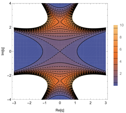
(a)

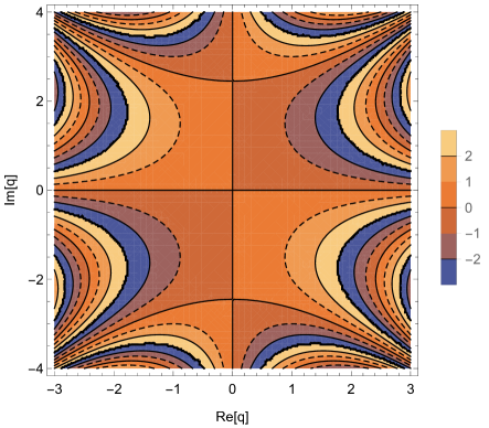
(b)

Figure 1: Modulus 1a and phase 1b of the integrand in (1) for $m^{2}+K=1$, $\lambda=1$. The integrand has a maximum at $q=0$ and saddles at $q=\pm im\sqrt{6/\lambda}$.

We introduce the conveniently rescaled variables $k=K/m^{2}$ and $\rho=3m^{4}/4\lambda$ and obtain

$$Z\left[K\right]=\frac{2N}{m}\sqrt{\rho\left(1+k\right)}\exp\left(\rho\left(1+k\right)^{2}\right)\mathrm{K}_{1/4}\left(\rho\left(1+k\right)^{2}\right),$$ (2)

where $K_{1/4}\left(\cdots\right)$ is a modified Bessel function of the second kind. This expression is valid so long as

$$\mathrm{Re}\left(\sqrt{\rho}\left(1+k\right)\right)>0,$$ (3)

which extends the definition (1) to the entirety of the cut $\lambda$-plane. The normalization factor is

$$N=\frac{m}{2}\frac{\exp\left(-\rho\right)}{\sqrt{\rho}\mathrm{K}_{1/4}\left(\rho\right)},$$ (4)

and finally

$$Z\left[K\right]=\sqrt{1+k}\exp\left(\rho\left[\left(1+k\right)^{2}-1\right]\right)\frac{\mathrm{K}_{1/4}\left(\rho\left(1+k\right)^{2}\right)}{\mathrm{K}_{1/4}\left(\rho\right)}.$$ (5)

$Z\left[K\right]$ is used to compute the expectation value of physical observables $O\left(q^{2}\right)$, by the standard trick of differentiating under the integral and then removing the source:

$$\left\langle O\left(q^{2}\right)\right\rangle \equiv N\int_{-\infty}^{\infty}\mathrm{d}q\ O\left(q^{2}\right)\exp\left(-\frac{1}{2}m^{2}q^{2}-\frac{1}{4!}\lambda q^{4}\right)$$

$$=\left.O\left(-2\partial_{K}\right)Z\left[K\right]\right|_{K=0}.$$ (6)

We also define the generating function

$$W\left[K\right]=-\ln Z\left[K\right]$$ (7)

and note that averages are found by taking derivatives of $W$. For example,

$$\frac{\partial}{\partial K}W\left[K\right] =\frac{1}{2}\left\langle q^{2}\right\rangle_{K}\equiv\frac{1}{2}\bar{G},$$ (8)

$$\frac{\partial^{2}}{\partial K^{2}}W\left[K\right] =-\frac{1}{4}\left(\left\langle q^{4}\right\rangle-\left\langle q^{2}\right\rangle^{2}\right)_{K}\equiv\frac{1}{4}\left(V^{\left(4\right)}\bar{G}^{4}-2\bar{G}^{2}\right),$$ (9)

where the subscript $K$ indicates the average is taken at a fixed value of $K$. (Note that $W\left[K\right]$ is not the connected generating function as usually defined because $K$ is a two-point source.) $\bar{G}$ and $V^{\left(4\right)}$ are the proper two and four point functions respectively. To lowest order in perturbation theory and with $K=0$, $\bar{G}=1/m^{2}+\mathcal{O}\left(\lambda\right)$ and $V^{\left(4\right)}=\lambda+\mathcal{O}\left(\lambda^{2}\right)$.

The exact value of $W\left[K\right]$ is easily obtained directly from the definition, giving

$$W\left[K\right] =-\frac{1}{2}\ln\left(1+k\right)-\rho\left[\left(1+k\right)^{2}-1\right]-\ln\mathrm{K}_{1/4}\left(\rho\left(1+k\right)^{2}\right)+\ln\mathrm{K}_{1/4}\left(\rho\right).$$ (10)

By direct differentiation we obtain the exact two point correlation function

$$m^{2}\left\langle q^{2}\right\rangle_{K} =4\rho\left(1+k\right)\left[\frac{\mathrm{K}_{3/4}\left(\rho\left(1+k\right)^{2}\right)}{\mathrm{K}_{1/4}\left(\rho\left(1+k\right)^{2}\right)}-1\right],$$ (11)

or for the original ($K=0$) theory,

$$m^{2}\bar{G} =4\rho\left(\frac{\mathrm{K}_{3/4}\left(\rho\right)}{\mathrm{K}_{1/4}\left(\rho\right)}-1\right).$$ (12)

Like $Z$, $\bar{G}$ possesses a branch cut discontinuity from $\lambda=0$ to $\lambda=-\infty$. At $\lambda=0$ one obtains the usual free (Gaussian) theory result $\bar{G}=G_{0}=m^{-2}$. In the strong coupling limit, $\lambda\to\infty$, $\bar{G}\sim\left[2\sqrt{6}\Gamma\left(\frac{3}{4}\right)/\Gamma\left(\frac{1}{4}\right)\right]\lambda^{-1/2}+\mathcal{O}\left(\lambda^{-1}\right)$. $\bar{G}$ is shown in Figure 2, from which the branch cut is obvious. This can also be seen in more detail in the complex $\lambda$ plane as shown in Figure 3. One sees that not only does $\bar{G}$ possess a branch cut, it is analytic in the cut plane and is in fact a Herglotz-Nevanlinna function (i.e. $\bar{G}\left(\lambda\right)^{\star}=\bar{G}\left(\lambda^{\star}\right)$ where $\star$ is complex conjugation). This means that $\bar{G}$ has a nice integral representation which we derive now in order to quantify the branch cut.

Figure 2: $\bar{G}$ from (12) as a function of $\lambda$ for $m=1$. The sign of the imaginary part depends on whether one approaches the $\lambda<0$ cut from above or below. Note the imaginary part is exponentially suppressed near the origin because the vacuum decay process is non-perturbative.

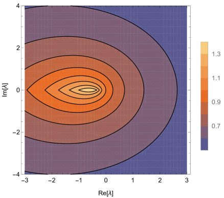
(a)

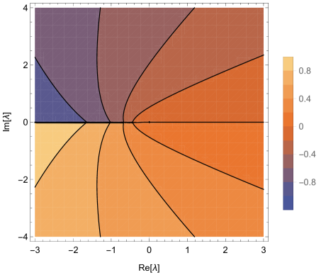
(b)

Figure 3: Modulus 3a and phase 3b of $\bar{G}$ in (12) for $m^{2}=1$ in the complex $\lambda$ plane.

We obtain the integral representation for $\bar{G}$ using the Cauchy formula

$$\bar{G}\left(\lambda\right)=\frac{1}{2\pi i}\oint_{C}\frac{\bar{G}\left(\lambda^{\prime}\right)}{\lambda^{\prime}-\lambda}\mathrm{d}\lambda^{\prime},$$ (13)

where the contour $C$ circles $\lambda$ in the counter-clockwise direction and avoids the cut. Deforming the contour to run on the circle at infinity and around the cut and using $\bar{G}\left(\lambda\right)\to 0$ as $\left|\lambda\right|\to\infty$, we can write the integral in terms of a spectral function $\sigma\left(s\right)=\left[\bar{G}\left(-s-i\epsilon\right)-\bar{G}\left(-s+i\epsilon\right)\right]\Theta\left(s\right)/2\pi i=\mathrm{Im}\left[\bar{G}\left(-s-i\epsilon\right)\right]\Theta\left(s\right)/\pi$ where $\Theta\left(s\right)$ is the Heaviside step function, such that

$$\bar{G}\left(\lambda\right)=\int_{0}^{\infty}\mathrm{d}s\frac{\sigma\left(s\right)}{s+\lambda}.$$ (14)

We find

$$\sigma\left(\lambda\right)=-\frac{4\sqrt{2}}{m^{2}\pi^{2}}\frac{1}{\mathrm{Im}\left[I_{-\frac{1}{4}}\left(-\rho\right)^{2}-I_{\frac{1}{4}}\left(-\rho\right)^{2}\right]}\Theta\left(\lambda\right),$$ (15)

where $I_{\pm\frac{1}{4}}\left(\rho\right)$ are modified Bessel functions of the first kind. $\sigma\left(\lambda\right)$ is shown in Figure 4.

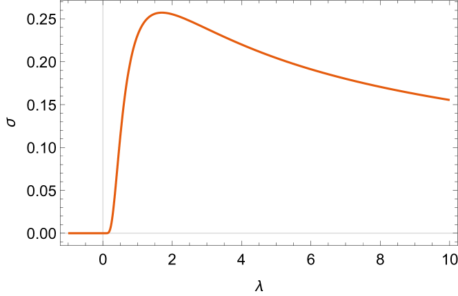
Figure 4: Spectral function $\sigma\left(\lambda\right)$ of (15) for $m=1$.

3 Perturbation theory and re-summations

3.1 Perturbation theory

At small coupling one often uses perturbation theory in $\lambda$ which proceeds by expanding the exponential

$$Z\left[K\right] =N\int_{-\infty}^{\infty}\mathrm{d}q\exp\left(-\frac{1}{2}\left(m^{2}+K\right)q^{2}-\frac{1}{4!}\lambda q^{4}\right)$$

$$=N\int_{-\infty}^{\infty}\mathrm{d}q\sum_{n=0}^{\infty}\frac{1}{n!}\left(-\frac{1}{4!}\lambda q^{4}\right)^{n}\exp\left(-\frac{1}{2}\left(m^{2}+K\right)q^{2}\right)$$

$$\sim\sum_{n=0}^{\infty}\frac{1}{n!}\left(-\frac{1}{4!}\lambda\right)^{n}N\int_{-\infty}^{\infty}\mathrm{d}qq^{4n}\exp\left(-\frac{1}{2}\left(m^{2}+K\right)q^{2}\right)$$

$$=\sum_{n=0}^{\infty}\frac{1}{n!}\left(-\frac{1}{4!}\lambda\right)^{n}N2^{2n+\frac{1}{2}}\Gamma\left(2n+\frac{1}{2}\right)\frac{1}{\left(m^{2}+K\right)^{2n+\frac{1}{2}}}.$$ (16)

In the third line we have formally interchanged the sum and integral, leading to an asymptotic rather than convergent series for $Z\left[K\right]$. Again, $N$ is determined by $Z\left[0\right]=1$, giving

$$N=\left[\sum_{n=0}^{\infty}\frac{1}{n!}\left(-\frac{1}{4!}\lambda\right)^{n}2^{2n+\frac{1}{2}}\Gamma\left(2n+\frac{1}{2}\right)\frac{1}{\left(m^{2}\right)^{2n+\frac{1}{2}}}\right]^{-1},$$ (17)

so

$$Z\left[K\right]=\frac{\sum_{n=0}^{\infty}\frac{1}{n!}\left(-\frac{1}{4!}\lambda\right)^{n}2^{2n}\Gamma\left(2n+\frac{1}{2}\right)\frac{1}{\left(m^{2}+K\right)^{2n+\frac{1}{2}}}}{\sum_{n=0}^{\infty}\frac{1}{n!}\left(-\frac{1}{4!}\lambda\right)^{n}2^{2n}\Gamma\left(2n+\frac{1}{2}\right)\frac{1}{\left(m^{2}\right)^{2n+\frac{1}{2}}}},$$ (18)

and

$$W\left[K\right]=-\ln\sum_{n=0}^{\infty}\frac{1}{n!}\left(-\frac{1}{4!}\lambda\right)^{n}2^{2n}\Gamma\left(2n+\frac{1}{2}\right)\frac{1}{\left(m^{2}+K\right)^{2n+\frac{1}{2}}}+\text{const}.$$ (19)

From this we find

$$\bar{G} =2\partial_{K}W$$

$$=\frac{1}{m^{2}}+\frac{4}{m^{2}}\frac{\sum_{n=1}^{\infty}\frac{1}{\left(n-1\right)!}\left(-\frac{1}{4!}\lambda\right)^{n}2^{2n}\Gamma\left(2n+\frac{1}{2}\right)\frac{1}{m^{4n}}}{\sum_{n=0}^{\infty}\frac{1}{n!}\left(-\frac{1}{4!}\lambda\right)^{n}2^{2n}\Gamma\left(2n+\frac{1}{2}\right)\frac{1}{m^{4n}}}$$

$$=\frac{1}{m^{2}}-\frac{\lambda}{2m^{6}}+\frac{2\lambda^{2}}{3m^{10}}-\frac{11\lambda^{3}}{8m^{14}}+\frac{34\lambda^{4}}{9m^{18}}+\cdots.$$ (20)

The perturbative approximations $G_{n}$ are the $\mathcal{O}\left(\lambda^{n}\right)$ truncations of this series. The first few are shown compared to the exact $\bar{G}$ in Figure 5. Note that these are simply the low order Taylor series approximations to $\bar{G}$. These approximations apparently converge poorly to the exact solution, and in fact we will shortly show that the series diverges.

The series for $\bar{G}$ can be described in terms of Feynman diagrams by the following rules:

1. Draw all connected graphs with two external lines (i.e. lines with one end not connected to any vertex) constructed from lines and four point vertices.

2. Associate to each line a factor $G_{0}=1/m^{2}$.

3. Associate to each vertex a factor $-\lambda$.

4. Divide by an overall symmetry factor being the order of the symmetry group of the diagram under permutations of lines and vertices.

We illustrate these rules by giving the first few terms in $\bar{G}$: perturbation-theory-propagator

$$\bar{G} =\parbox{42.67912pt}{\fmfgraph(15,15) \fmfleft{i}\fmfright{o}\fmf{plain}{i,o}}+\frac{1}{2}\parbox{42.67912pt}{\fmfgraph(15,15) \fmfleft{i}\fmfright{o}\fmf{plain}{i,v,v,o} \fmfdot{v}}+\frac{1}{4}\parbox{56.9055pt}{\fmfgraph(20,15) \fmfleft{i}\fmfright{o}\fmf{plain}{i,v1,v1,v2,v2,o} \fmfdot{v1}\fmfdot{v2}}+\frac{1}{4}\parbox{56.9055pt}{\fmfgraph(20,15) \fmfleft{i}\fmfright{o}\fmftop{t} \fmf{plain}{i,v1,o}\fmffreeze\fmf{phantom}{v1,v2} \fmf{phantom}{v2,t}\fmffreeze\fmf{plain,left}{v1,v2,t,v2,v1} \fmfdot{v1,v2}}+\frac{1}{6}$$

$$+\frac{1}{8}\parbox{71.13188pt}{ \fmfgraph(25,15) \fmfleft{i}\fmfright{o} \fmf{plain}{i,v1,v1,v2,v2,v3,v3,o} \fmfdot{v1,v2,v3} }+\frac{1}{8}\parbox{71.13188pt}{ \fmfgraph(25,15) \fmfleft{i}\fmfright{o}\fmftop{tl,t1,t2,tr} \fmf{plain}{i,v1,v2,o}\fmffreeze\fmf{phantom}{v1,x1,t1}\fmffreeze\fmf{phantom}{v2,v3,t2}\fmffreeze\fmf{plain,left}{v1,x1,v1} \fmf{plain,left}{v2,v3,v2} \fmf{plain,left}{v3,t2,v3} \fmfdot{v1,v2,v3} }+\frac{1}{8}\parbox{71.13188pt}{ \fmfgraph(25,15) \fmfleft{i}\fmfright{o}\fmftop{tl,t2,t1,tr} \fmf{plain}{i,v2,v1,o}\fmffreeze\fmf{phantom}{v1,x1,t1}\fmffreeze\fmf{phantom}{v2,v3,t2}\fmffreeze\fmf{plain,left}{v1,x1,v1} \fmf{plain,left}{v2,v3,v2} \fmf{plain,left}{v3,t2,v3} \fmfdot{v1,v2,v3} }$$

$$+\frac{1}{12}\parbox{71.13188pt}{ \fmfgraph(25,20) \fmfleft{i}\fmfright{o} \fmf{plain}{i,v1,v1,v2,v3,o} \fmf{plain,left,tension=0}{v2,v3,v2} \fmfdot{v1,v2,v3} }+\frac{1}{12}\parbox{71.13188pt}{ \fmfgraph(25,20) \fmfleft{i}\fmfright{o} \fmf{plain}{i,v2,v3,v1,v1,o} \fmf{plain,left,tension=0}{v2,v3,v2} \fmfdot{v1,v2,v3} }+\frac{1}{8}\parbox{71.13188pt}{ \fmfgraph(25,20) \fmfleft{i}\fmfright{o}\fmftop{t} \fmf{plain}{i,v1,o}\fmffreeze\fmf{phantom}{v1,v2,v3,t}\fmffreeze\fmf{plain,left}{v1,v2,v3,t,v3,v2,v1} \fmfdot{v1,v2,v3} }$$

$$+\frac{1}{12}\parbox{71.13188pt}{ \fmfgraph(25,25) \fmfleft{i}\fmfright{o}\fmftop{tl,t1,t2,tr} \fmf{plain}{i,x1,v1,x2,o}\fmffreeze\fmf{phantom}{x1,v2,t1}\fmffreeze\fmf{phantom}{x2,v3,t2}\fmffreeze\fmf{plain,left=0.5}{v1,v2} \fmf{plain,right=0.5}{v1,v3} \fmf{plain,left=0.5}{v2,v3,v2} \fmf{plain}{v2,v3} \fmfdot{v1,v2,v3} }+\frac{1}{4}\parbox{71.13188pt}{ \fmfgraph(25,25) \fmfleft{i}\fmfright{o}\fmftop{t} \fmf{plain}{i,v1,v2,o}\fmffreeze\fmf{plain,left=0.5}{v1,v3,v2} \fmf{plain,right}{v1,v2} \fmf{phantom,tension=0.1}{v3,t} \fmf{plain,left}{v3,t,v3} \fmfdot{v1,v2,v3} }+\frac{1}{8}\parbox{71.13188pt}{ \fmfgraph(25,25) \fmfleft{lm2,lm1,i,l1,l2}\fmfright{rm2,rm1,o,r1,r2}\fmftop{tl,t1,t2,t3,tr} \fmf{plain}{i,v1,o}\fmffreeze\fmf{phantom}{l1,v2,v3,r1}\fmffreeze\fmf{plain,left=0.6}{v1,v2} \fmf{plain,left=0.4}{v2,v3} \fmf{plain,left=0.6}{v3,v1} \fmf{plain,left}{v2,t1,v2}\fmf{plain,left}{v3,t3,v3} \fmfdot{v1,v2,v3} }$$

$$+\frac{1}{4}\parbox{71.13188pt}{ \fmfgraph(25,15) \fmfleft{i}\fmfright{o}\fmftop{t} \fmf{plain}{i,v1,x1,v2,o}\fmffreeze\fmf{phantom}{t,v3,x1}\fmffreeze\fmf{plain,right=0.3}{v1,v3,v2} \fmf{plain,left=0.5}{v1,v3,v2} \fmfdot{v1,v2,v3} }+\mathcal{O}\left(\lambda^{4}\right).$$ (21)

$W\left[K\right]$ can be written as a similar diagrammatic series in terms of connected vacuum diagrams (i.e., those with no external lines).

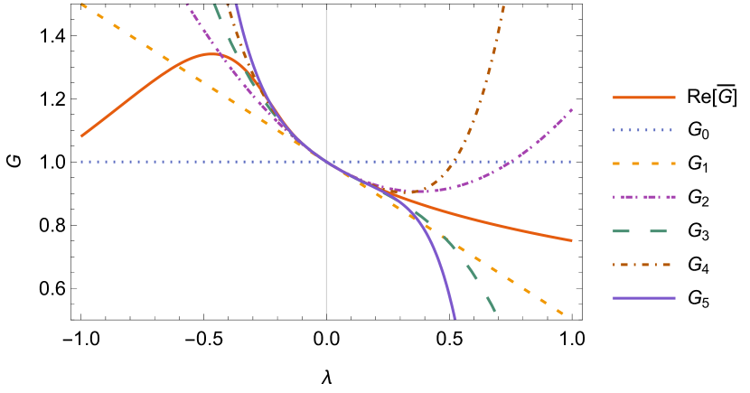
Figure 5: Perturbative approximations to $\bar{G}$ up to $\mathcal{O}\left(\lambda^{5}\right)$ for $m=1$, compared to the exact solution.

The series (20) has the form $\bar{G}=m^{-2}\sum_{n=0}^{\infty}c_{n}\left(\lambda/m^{4}\right)^{n}$ where the coefficients asymptotically obey $c_{n+1}\sim-\frac{2}{3}nc_{n}$ as $n\to\infty$, thus the radius of convergence of the series is zero. This is consistent with the fact that we are perturbing around a branch point of the exact solution: no approximation of $\bar{G}$ in terms of analytic functions can converge at $\lambda=0$ because $Z\left[K\right]$ is itself undefined for $\mathrm{Re}\lambda<0$. The terms of the series start to increase when $c_{n+1}\left(\lambda/m^{4}\right)\sim c_{n}$, i.e. $n\sim 3m^{4}/2\lambda$, meaning the series is useful for $\lambda\ll m^{4}$ but fails immediately for a moderately strong coupling $\lambda\approx m^{4}$. This is typical asymptotic series behaviour as shown in Figure 6. Extrapolating perturbation theory to strong coupling $\lambda\gg m^{4}$ is simply impossible, although the exact solution is well behaved there. (In fact $\bar{G}$ can be expanded as $\bar{G}=m^{-2}\sum_{n=1}^{\infty}\tilde{c}_{n}\left(\lambda/m^{4}\right)^{-n/2}$, displaying explicitly the branch point at $\lambda=\infty$.)

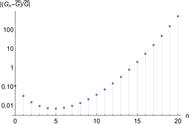
Figure 6: Relative error $\left|\left(G_{n}-\bar{G}\right)/\bar{G}\right|$of the $n$-th perturbative approximation to $\bar{G}$ for $m=1$ and $\lambda=1/4$, showing the decreasing then increasing behaviour typical of asymptotic series.

3.2 Borel summation

We have seen that the series expansion for $\bar{G}$ diverges for all $\lambda\neq 0$. This is typical of perturbation series and usually signals some singularity of the exact solution for unphysical values of $\lambda$. In our case, indeed, the theory does not exist for $\mathrm{Re}\lambda<0$ and the exact solution possesses a branch cut on the negative $\lambda$ axis, a feature which cannot be reproduced in any order of perturbation theory. However, the perturbation series is asymptotic and does contain true information about the exact solution, even if $\lambda$ is large enough that the series is not useful practically. Because of the ubiquity of this phenomenon, mathematicians have invented a number of series summation techniques which assign a finite value to certain types of divergent series and which obey certain consistency properties (e.g. the value assigned to a convergent series is just its naïve sum). Here we investigate Borel summation, which is capable of summing factorially divergent series like (20).

Suppose that $\sum_{n=0}^{\infty}a_{n}$ is a divergent series but that the Borel transform of the series, defined as

$$\phi\left(x\right)=\sum_{n=0}^{\infty}\frac{a_{n}x^{n}}{n!},$$ (22)

converges for sufficiently small $x$. Then, if the integral

$$B\left(x\right)=\int_{0}^{\infty}\mathrm{e}^{-t}\phi\left(xt\right)\mathrm{d}t$$ (23)

exists the Borel sum [16, 17, 18] of the divergent series is defined as $\mathcal{B}\left[\sum_{n=0}^{\infty}a_{n}\right]\equiv B\left(1\right)$. This definition is justified by substituting the series for $\phi\left(xt\right)$ into the integral and evaluating term-wise and noting that $B\left(x\right)\sim\sum_{n=0}^{\infty}a_{n}x^{n}$. The main drawback of Borel summation is that one must know the precise form of $a_{n}$ for all $n$ to compute $\phi\left(x\right)$, which is rarely the case in field theory. For this reason Borel summation cannot be usefully applied directly. However, one may use Padé approximants as discussed in the next section to recast the Borel transform in a useful way.

We note that the key to Borel-summability of the perturbation series is the alternating sign $\left(-1\right)^{n}$ of the $n$-th order term. To see this consider the two series

$$S_{1} =\sum_{n=0}^{\infty}\left(-\lambda\right)^{n}n!,$$ (24)

$$S_{2} =\sum_{n=0}^{\infty}\lambda^{n}n!,$$ (25)

which differ only by the alternating sign. The Borel transforms $\phi_{1,2}\left(x\right)$ are

$$\phi_{1}\left(x\right) =\sum_{n=0}^{\infty}\left(-\lambda x\right)^{n}=\frac{1}{1+\lambda x},$$ (26)

$$\phi_{2}\left(x\right) =\sum_{n=0}^{\infty}\left(\lambda x\right)^{n}=\frac{1}{1-\lambda x},$$ (27)

and the Borel sums are

$$\mathcal{B}\left[S_{1}\right]=B_{1}\left(1\right) =\int_{0}^{\infty}\frac{\mathrm{e}^{-t}}{1+\lambda t}\mathrm{d}t,$$ (28)

$$\mathcal{B}\left[S_{2}\right]=B_{2}\left(1\right) =\int_{0}^{\infty}\frac{\mathrm{e}^{-t}}{1-\lambda t}\mathrm{d}t.$$ (29)

In the first case the integral exists and $\mathcal{B}\left[S_{1}\right]=\lambda^{-1}\mathrm{e}^{1/\lambda}\Gamma\left(0,\frac{1}{\lambda}\right)$ where $\Gamma\left(a,b\right)=\int_{b}^{\infty}t^{a-1}\mathrm{e}^{-t}\mathrm{d}t$ is the incomplete gamma function. However, the second integral hits a pole at $t=1/\lambda$. There is no natural prescription for avoiding the pole, which leads to an ambiguity in the sum of $\pm\pi i\lambda^{-1}\mathrm{e}^{-1/\lambda}$. This is a non-perturbative ambiguity called a renormalon [19]. In every known case where this arises in field theory the renormalon is connected to a non-perturbative finite action solution of the field equations, i.e. an instanton or soliton, and a correct evaluation of the path integral which sums over all saddle points (not just perturbative ones) removes the ambiguity. Key to the practical application of Borel summation is the location and classification of all renormalons in a given theory [15]. Sophisticated techniques have been developed to deal with this situation which are beyond the scope of this paper [18, 20, 21].

3.3 Padé approximation

Borel summation on its own has limited usefulness in practice because one often only knows a few low order terms of perturbation theory, and the potential existence of renormalon singularities. There exists another technique which often improves perturbation series and is far more useful in practice (and is often combined with Borel summation). Padé approximation approximates a function by rational polynomials which generally converge rapidly, are very useful for numerical computation and help to estimate the location of singularities of the function in the complex plane. Many software packages include standard routines for evaluating Padé approximants, for instance the PadeApproximant function in Mathematica. In this section we apply Padé approximants directly to the Green function and then to the Borel transform. We find that the latter approach is clearly the better one.

The $\left(N,M\right)$-Padé approximant of a function $\sum_{n=0}^{\infty}a_{n}x^{n}$ is given by [16]

$$P_{M}^{N}\left(x\right)=\frac{\sum_{n=0}^{N}A_{n}x^{n}}{\sum_{n=0}^{M}B_{n}x^{n}},$$ (30)

where without loss of generality one takes $B_{0}=1$. The remaining $N+M+1$ coefficients are chosen so that the Taylor series of $P_{M}^{N}\left(x\right)$ matches the perturbation series up to $\mathcal{O}\left(x^{N+M}\right)$. Due to the denominator, Padé approximants develop poles in the complex $x$-plane, allowing the close approximation of more singular functions than Taylor series are capable of. Examples of the use of Padé approximants in field theory can be found in [17, 22] and references therein.

Now we find the Padé approximants to $m^{2}\bar{G}$ with $x=\lambda/m^{4}$. Here we restrict attention to the approximants where $M=N+1$. This guarantees that $P_{M}^{N}\to 0$ as $\lambda\to\infty$. If we had used the usual diagonal approximants ($N=M$) we would find an unphysical constant term $P_{N}^{N}\to A_{N}/B_{N}$ as $\lambda\to\infty$. Note that it is impossible to match the true $1/\sqrt{\lambda}$ behaviour of $\bar{G}$ as $\lambda\to\infty$ using Padé approximants centred on the origin. The best that is possible in this limit is $\sim\lambda^{-1}$. (As it happens, using $x\propto\sqrt{\lambda}$ does not allow one to resolve this issue: the same approximants are found only with $x^{2}$ everywhere in place of $x$. This is because the $1/\sqrt{\lambda}$ behaviour is due to the branch point at infinity, which is infinitely far from the origin where the Padé approximants are matched to perturbation theory. Low order Padé approximants can extract information about the branch point near the origin, but evidently not the one at infinity.) The first five approximants for $m^{2}\bar{G}$ are shown in Table 1 and the first three are plotted in Figure 7 with comparison to the exact $\bar{G}$. Note that the existence of the integral representation (14) for $\bar{G}$ implies that $\bar{G}$ is a Stieltjes function, meaning one can prove convergence properties for the Padé approximants as $N,M\to\infty$, though we are not concerned with this analysis here (see [16] for details).

Table 1: First few Padé approximants for $m^{2}\bar{G}$.

$N$	$P_{N+1}^{N}$
0	$\begin{aligned} \frac{1}{1+\frac{\lambda}{2m^{4}}}\end{aligned}$
1	$\begin{aligned} \frac{1+\frac{2\lambda}{m^{4}}}{1+\frac{5\lambda}{2m^{4}}+\frac{7\lambda^{2}}{12m^{8}}}\end{aligned}$
2	$\begin{aligned} \frac{1+\frac{16\lambda}{3m^{4}}+\frac{59\lambda^{2}}{12m^{8}}}{1+\frac{35\lambda}{6m^{4}}+\frac{43\lambda^{2}}{6m^{8}}+\frac{77\lambda^{3}}{72m^{12}}}\end{aligned}$
3	$\begin{aligned} \frac{1+\frac{10\lambda}{m^{4}}+\frac{155\lambda^{2}}{6m^{8}}+\frac{15\lambda^{3}}{m^{12}}}{1+\frac{21\lambda}{2m^{4}}+\frac{365\lambda^{2}}{12m^{8}}+\frac{295\lambda^{3}}{12m^{12}}+\frac{385\lambda^{4}}{144m^{16}}}\end{aligned}$
4	$\begin{aligned} \frac{1+\frac{16\lambda}{m^{4}}+\frac{315\lambda^{2}}{4m^{8}}+\frac{1190\lambda^{3}}{9m^{12}}+\frac{7945\lambda^{4}}{144m^{16}}}{1+\frac{33\lambda}{2m^{4}}+\frac{259\lambda^{2}}{3m^{8}}+\frac{11935\lambda^{3}}{72m^{12}}+\frac{14315\lambda^{4}}{144m^{16}}+\frac{7315\lambda^{5}}{864m^{20}}}\end{aligned}$

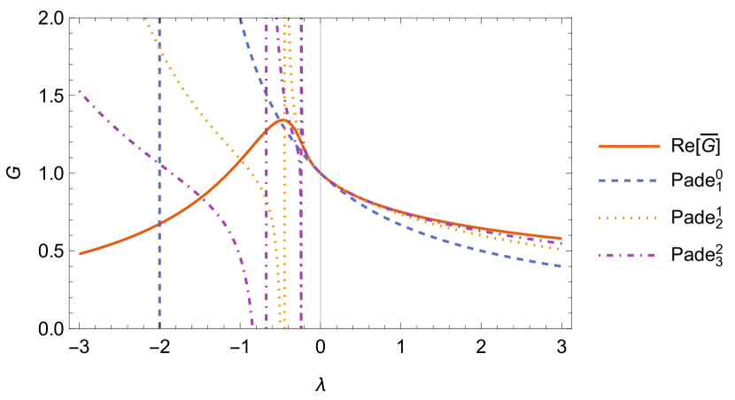
Figure 7: First three Padé approximants to $\bar{G}$. Note the simple poles developed for $\lambda<0$.

The $\left(N,N+1\right)$-Padé approximant can also be written as

$$P_{N+1}^{N}=\sum_{i=0}^{N}\frac{r_{i}}{\lambda-p_{i}},$$ (37)

where $r_{i}$ and $p_{i}$ are the $i$-th residue and pole respectively. Note that since all of the coefficients in the denominators of Table 1 are positive and real, all of the poles must either be on the negative real axis or they must be complex and come in complex conjugate pairs. Numerical experiments suggest that all the poles lie on the negative $\lambda$ axis, though we do not know a proof of this for all $N$. Assuming this is generally true, Padé approximants give a representation of $\bar{G}$ which approximates the continuous spectral function by a sum of delta functions

$$\sigma\left(s\right)\approx\sigma_{N}\left(s\right)\equiv\sum_{i=0}^{N}r_{i}\delta\left(s+p_{i}\right).$$ (38)

As $N\to\infty$ the poles become denser and fill the negative $\lambda$ axis, eventually merging into a continuous branch cut. Similarly the spectral function turns into a dense sum of delta functions which, when considered acting on any sufficiently smooth test function, smooths into a continuous function. The first few $\sigma_{N}$ are shown next to the exact spectral function in Figure 8 for comparison.

Figure 8: Padé approximations to the spectral function $\sigma\left(\lambda\right)$ consist of an increasingly dense set of delta functions. (Note the delta functions have been smoothed for visual purposes only.)

Now we consider Padé approximation of the Borel transform of $\bar{G}$. First we note the following connections between the Borel transform $\phi$ and $\bar{G}$ and $\sigma$:

$$v^{-1}\sigma\left(\frac{\lambda}{v}\right)\xleftarrow[x\to v]{\mathcal{L}^{-1}}\phi\left(x\right)\xrightarrow[x\to s]{\mathcal{L}}s^{-1}\bar{G}\left(\frac{\lambda}{s}\right).$$ (39)

That is, the Green function is related to the Laplace transform of the Borel transform, while the spectral function is related to the inverse Laplace transform of the Borel transform. These relations can be shown using the definitions of $\phi$ and $\sigma$ and the integral representation of the (inverse) Laplace transform. This allows us to extract the spectral function directly from the Borel transform. Note that each pole of $\phi$ yields by the inverse Laplace transform a term of the form $\lambda^{-1}\exp{\left(-k/\lambda\right)}$ in $\sigma$, where $k$ is controlled by the location of the pole. The general Borel-Padé approximation for $\sigma$ is a superposition of terms of this form.

We show the first few approximants to $\bar{G}$ and $\sigma$ in Figures 9 and 10 respectively. One sees that the low order Borel-Padé Green functions are reasonably accurate (within a few percent for $\lambda\leq 5m^{4}$) but the spectral functions are not approximated particularly well. Certain approximants to $\sigma$ oscillate erratically and even become negative for certain values of $\lambda$. Except for the fact that the best approximant is the highest order one plotted, there is no clear sense in which the Borel-Padé approximations appear to converge to $\sigma$. However, even this bad approximation is at least a continuous function, as opposed to a sum of delta functions.

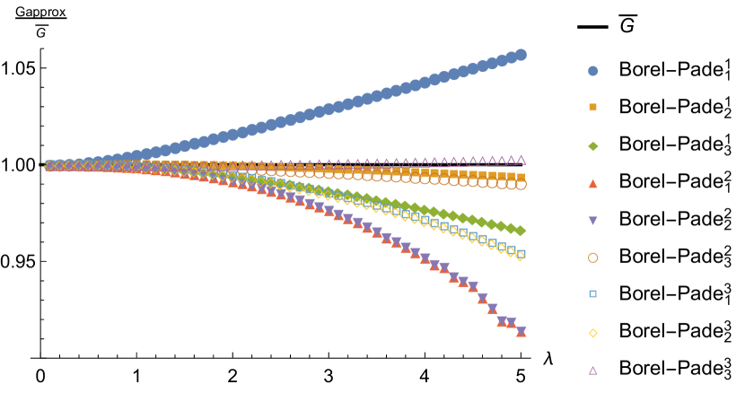
Figure 9: Borel-Padé approximations to the Green function $\bar{G}\left(\lambda\right)$ (ratio of approximant / exact). Approximants are calculated by numerical integration of (23).

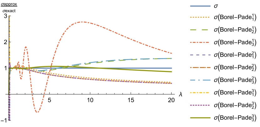
Figure 10: Borel-Padé approximations to the spectral function $\sigma\left(\lambda\right)$ (ratio of approximant / exact). Note that the (2,2) approximant is off scale.

4 2PI Approximations

The 2PI effective action is a functional of the Green function $G\equiv\left\langle q^{2}\right\rangle_{K}$ which is defined by the Legendre transform [5, 4]

$$\Gamma\left[G\right]=W\left[K\right]-K\partial_{K}W\left[K\right]$$ (40)

where $K$ is solved for in terms of $G$. $\Gamma\left[G\right]$ obeys the equation of motion

$$\partial_{G}\Gamma\left[G\right]=-\frac{1}{2}K.$$ (41)

The standard derivation of the 2PI action [5, 4] gives in this case

$$\Gamma\left[G\right]=\frac{1}{2}\ln\left(G^{-1}\right)+\frac{1}{2}m^{2}G+\gamma_{2\mathrm{PI}}+\mathrm{const.},$$ (42)

where $-\gamma_{2\mathrm{PI}}$ is (minus due to Euclidean conventions) the sum of two particle irreducible vacuum graphs, i.e. those graphs which do not fall apart when any two lines are cut, where the lines are given by $G$ and vertices by $-\lambda$. Explicitly:twopi-diagrams

$$-\gamma_{2\text{PI}} =\frac{1}{8}\ \parbox[c]{42.67912pt}{\fmfgraph(15,20) \fmfleft{l}\fmfright{r} \fmf{plain,left}{l,v,r,v,l} \fmfdot{v} }\ +\frac{1}{4!2}\ \parbox{28.45274pt}{\fmfgraph(10,20) \fmfleft{l}\fmfright{r} \fmf{plain,left}{l,r,l} \fmf{plain,left=0.5}{l,r,l} \fmfdot{l,r} }\ +\frac{1}{2^{3}3!}\parbox{28.45274pt}{\fmfgraph(10,10) \fmfsurroundn{v}{3} \fmfdotn{v}{3} \fmfcyclen{plain,right=0.25}{v}{3} \fmfrcyclen{plain,right=0.25}{v}{3} }+\mathcal{O}\left(\lambda^{4}\right)$$

The equation of motion in the absence of sources is

$$G^{-1}=m^{2}+2\partial_{G}\gamma_{2\mathrm{PI}},$$ (43)

which has the diagram expansion 2pi-eom

$$G^{-1}=m^{2}-\frac{1}{2}\ \parbox{42.67912pt}{\fmfgraph(15,15) \fmfleft{i}\fmfright{o}\fmf{plain}{i,v,v,o} \fmfdot{v}}\ -\frac{1}{6}\ \parbox{56.9055pt}{\fmfgraph(20,15) \fmfleft{i}\fmfright{o} \fmf{plain}{i,v1,v2,o} \fmf{plain,left,tension=0}{v1,v2,v1} \fmfdot{v1,v2}}\ -\frac{1}{4}\parbox{71.13188pt}{ \fmfgraph(25,20) \fmfleft{i}\fmfright{o}\fmftop{t} \fmf{plain}{i,v1,x1,v2,o}\fmffreeze\fmf{phantom}{t,v3,x1}\fmffreeze\fmf{plain,right=0.3}{v1,v3,v2} \fmf{plain,left=0.5}{v1,v3,v2} \fmfdot{v1,v2,v3} }+\mathcal{O}\left(\lambda^{4}\right).$$ (44)

Notice that there is a dramatic reduction in the number of graphs of a given order compared to perturbation theory (21) due to the two-particle irreducibility. This is one of the major benefits of 2PI approximation schemes in realistic theories, such as gauge theories, where the Feynman diagrams proliferate rapidly.

The equation of motion is Dyson’s equation and the second term on the right hand side, $-\Sigma=2\partial_{G}\gamma_{2\mathrm{PI}}$, represents the exact one-particle irreducible self-energy of the propagator $G$. This can be put into the usual form of a Dyson equation by noting $m^{2}=G_{0}^{-1}$ and multiplying both sides by $GG_{0}$:

$$G=G_{0}+G_{0}\Sigma G.$$ (45)

Iterating this gives the infinite series

$$G=G_{0}+G_{0}\Sigma G_{0}+G_{0}\Sigma G_{0}\Sigma G_{0}+\cdots.$$ (46)

The main difference between this and the usual perturbative Dyson equation is that $\Sigma$ contains exact propagators $G$ rather than $G_{0}$. Inserting the expression above for $G$ into $\Sigma$ one finds that, even if one retains only a finite number of 2PI diagrams in $\gamma_{2\text{PI}}$, $\Sigma$ contains an infinite series of perturbative self-energy graphs. This is the motivation in the literature for talking about 2PI as a resummation method.

By power counting (or counting line ends in the corresponding diagrams) we find $\gamma_{2\mathrm{PI}}=\sum_{n=0}^{\infty}\gamma_{n}\left(\lambda G^{2}\right)^{n}$. It is possible to derive the $\gamma_{n}$ by considering the symmetry factors of the two particle irreducible Feynman diagrams, but we can also obtain the $\gamma_{n}$ in a simple automated way using knowledge of the exact solution $G=\bar{G}$. Substituting $\bar{G}$ into the equation of motion and the expansion for $\gamma_{2\text{PI}}$, expanding about $\lambda=0$ and matching powers of $\lambda$ we can determine

$$\gamma_{2\mathrm{PI}} =\frac{G^{2}\lambda}{8}-\frac{G^{4}\lambda^{2}}{48}+\frac{G^{6}\lambda^{3}}{48}-\frac{5G^{8}\lambda^{4}}{128}+\frac{101G^{10}\lambda^{5}}{960}-\frac{93G^{12}\lambda^{6}}{256}$$

$$+\frac{8143G^{14}\lambda^{7}}{5376}-\frac{271217G^{16}\lambda^{8}}{36864}+\frac{374755G^{18}\lambda^{9}}{9216}-\frac{5151939G^{20}\lambda^{10}}{20480}$$

$$+\frac{697775057G^{22}\lambda^{11}}{405504}-\frac{3802117511G^{24}\lambda^{12}}{294912}+\frac{201268707239G^{26}\lambda^{13}}{1916928}$$

$$-\frac{11440081763125G^{28}\lambda^{14}}{12386304}+\frac{5148422676667G^{30}\lambda^{15}}{589824}-\frac{1665014342007385G^{32}\lambda^{16}}{18874368}$$

$$+\frac{4231429245358235G^{34}\lambda^{17}}{4456448}-\frac{921138067678697395G^{36}\lambda^{18}}{84934656}+\mathcal{O}\left(\lambda^{19}G^{38}\right).$$ (47)

We do not know of any closed form expression for either the coefficients of this series or its sum (implicit analytic expressions can be derived; however, these require the inversion of $G=\bar{G}\left(\lambda\right)$ for $\lambda\left(G\right)$, which is not known to us in closed form). However, after the first few terms the coefficients seem to be well approximated by $\gamma_{i+1}\sim-\frac{2}{3}i\gamma_{i}$, the same as for the perturbation series. This has the hallmark of an asymptotic series. Like perturbation theory, the 2PI series does not converge.

The first non-trivial contribution to the equation of motion gives

$$G_{\left(1\right)}^{-1}=m^{2}+\frac{\lambda}{2}G_{\left(1\right)},$$ (48)

where the subscript $\left(1\right)$ indicates terms of order $\mathcal{O}\left(\lambda^{1}\right)$ have been kept. This has two solutions

$$G_{\left(1\right)}=\frac{-m^{2}\pm\sqrt{m^{4}+2\lambda}}{\lambda}.$$ (49)

One of these solutions is unphysical and we must choose the $+$ sign. As $\lambda\to 0$,

$$G_{\left(1\right)}\to\frac{1}{m^{2}}-\frac{\lambda}{2m^{6}}+\frac{\lambda^{2}}{2m^{10}}+\mathcal{O}\left(\lambda^{3}\right),$$ (50)

which matches perturbation theory up to $\mathcal{O}\left(\lambda^{2}\right)$ terms as expected. However, unlike perturbation theory, the strong coupling limit $\lambda\to\infty$ exists and gives

$$G_{\left(1\right)}\to\sqrt{\frac{2}{\lambda}}-\frac{m^{2}}{\lambda}+\frac{m^{4}}{\left(2\lambda\right)^{3/2}}+\mathcal{O}\left(\frac{1}{\lambda^{5/2}}\right).$$ (51)

This series has the correct form in powers of $\lambda^{-1/2}$, though the leading coefficient is incorrect by $\approx 15\%$, and the sub-leading coefficients are incorrect by $\approx 40\%$, $70\%$ and $100\%$ etc. Nevertheless, it is remarkable to achieve any accuracy at all given the simple nature of the approximation and the fact that $\gamma_{2\text{PI}}$ was truncated at leading order in $\lambda$! $G_{\left(1\right)}$ is a much more uniform approximation to $\bar{G}$ than the perturbative approximation $m^{-2}-\lambda/2m^{6}$.

This result is possible because of the branch cut $G_{\left(1\right)}$ possesses on the negative $\lambda$ axis. The discontinuity across the cut

$$G_{\left(1\right)}\left(\lambda+i\epsilon\right)-G_{\left(1\right)}\left(\lambda-i\epsilon\right)=2i\frac{\sqrt{-m^{4}-2\lambda}}{\lambda}\Theta\left(-\lambda-\frac{m^{4}}{2}\right),$$ (52)

gives the spectral function

$$\sigma_{\left(1\right)}\left(\lambda\right)=\frac{\sqrt{-m^{4}+2\lambda}}{\pi\lambda}\Theta\left(\lambda-\frac{m^{4}}{2}\right).$$ (53)

This is a far better approximation to the exact spectral function than obtained from any of the other techniques, as can be seen from Figure 11.

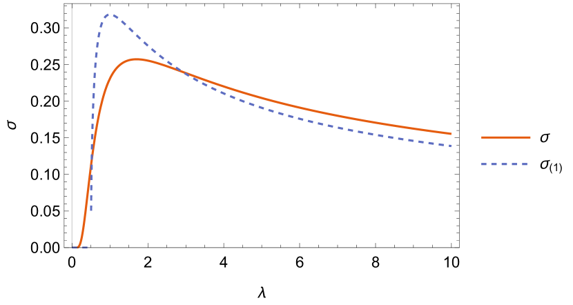
Figure 11: Comparison of exact spectral function $\sigma\left(\lambda\right)$ (15) with the two loop 2PI approximation $\sigma_{\left(1\right)}\left(\lambda\right)$ (53) for $m=1$. Already, the simplest nontrivial 2PI truncation gives a much better approximation than perturbation theory or Padé approximants to arbitrary order.

We show all of the first order approximations in Figure 12. Note that for $\lambda/m^{4}\geq 0$ the best approximation is the 2PI, followed by the Borel-Padé, then by Padé, then perturbation theory last of all. The situation for negative $\lambda$ is complicated. The best approximation overall is the 2PI, though it has an unphysical cusp where the branch cut starts ($\lambda/m^{4}=-1/2$ in Figure 12). It appears the 2PI approximation trades sensitivity to the exponentially small portion of $\sigma$ in exchange for a better global approximation. The Padé approximation is good at small negative $\lambda$ but hits a pole at $\lambda/m^{4}=-2$ and there loses all validity. The Borel-Padé approximation is smooth and more accurate than the 2PI near the peak of $\bar{G}$, but eventually becomes invalid, even negative, at sufficiently large negative $\lambda$ ($\lambda/m^{4}\lesssim-5.37$).

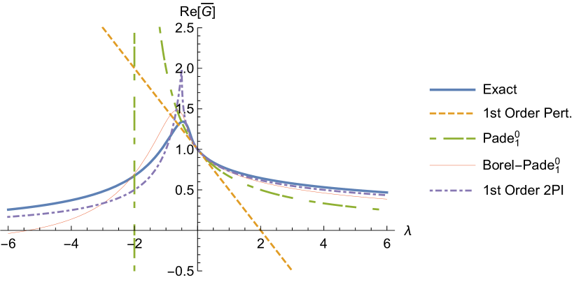
Figure 12: Comparison of (the real part of) the exact Green function $\bar{G}$ to each of the approximations discussed to first non-trivial order in each case.

At $n$-th order, (43) is a degree $2n$ polynomial in $G$ which has $2n$ roots, only one of which is physical. For $n=2$ there are analytical expressions for the roots, though they are very bulky, and for $n\geq 3$ (43) must be solved numerically. Picking out the correct root for a given value of $\lambda$ is tricky in general and we leave this exercise to the reader. However, one can see on general grounds that truncations of (43) give a singular perturbation theory in $\lambda$: at $\lambda=0$ the physical solution starts at $G_{0}$ and the spurious solutions flow in from infinity as inverse powers of $\lambda$ as $\lambda$ increases to finite values. At strong coupling the roots generically approach each other and one must carefully track them through the complex plane. We suspect that a resummation of the 2PI series would remove some or all of these spurious solutions, though we do not have a proof of this. We examine two potential methods to achieve this in the next section and find mixed results.

5 Hybrid 2PI-Padé

Since the series of 2PI diagrams is asymptotic, we may consider using a series summation method to improve convergence. Note that this is logically independent of the resummations embodied in the 2PI approximation itself. We may perform Padé summation of the action term $\gamma_{2\text{PI}}$ or the equation of motion term $\partial_{G}\gamma_{2\text{PI}}$. We consider both. First, consider Padé summation of the action which matches the series expansion up to order $N+M$:

$$\Gamma\left[G\right]=\frac{1}{2}\ln\left(G^{-1}\right)+\frac{1}{2}m^{2}G+\frac{\sum_{n=0}^{N}A_{n}^{\left(\gamma\right)}\left(\lambda G^{2}\right)^{n}}{\sum_{n=0}^{M}B_{n}^{\left(\gamma\right)}\left(\lambda G^{2}\right)^{n}}+\mathrm{const.}$$ (54)

The equation of motion becomes

$$G^{-1} =m^{2}+2\frac{\mathrm{d}}{\mathrm{d}G}\frac{\sum_{n=0}^{N}A_{n}^{\left(\gamma\right)}\left(\lambda G^{2}\right)^{n}}{\sum_{n=0}^{M}B_{n}^{\left(\gamma\right)}\left(\lambda G^{2}\right)^{n}}$$

$$=m^{2}+\frac{4\sum_{n=0}^{N}\sum_{k=0}^{M}\left(n-k\right)A_{n}^{\left(\gamma\right)}B_{k}^{\left(\gamma\right)}\lambda^{n+k}G^{2\left(n+k\right)-1}}{\left[\sum_{n=0}^{M}B_{n}^{\left(\gamma\right)}\left(\lambda G^{2}\right)^{n}\right]^{2}}.$$ (55)

Multiplying by the denominator this becomes a polynomial equation of degree $2\left(N+M\right)$ as expected. This equation will have $2\left(N+M\right)-1$ spurious solutions as does the ordinary 2PI approximation of matching order.

To take a specific example, consider $\gamma_{2\text{PI}}$ up to $\mathcal{O}\left(\lambda^{4}\right)$ and the matching $\left(2,2\right)$- and $\left(1,3\right)$-Padé approximants:

$$\gamma_{2\text{PI}} =\frac{G^{2}\lambda}{8}-\frac{G^{4}\lambda^{2}}{48}+\frac{G^{6}\lambda^{3}}{48}-\frac{5G^{8}\lambda^{4}}{128}+\cdots$$ (56)

$$\approx\frac{\frac{G^{2}\lambda}{8}+\frac{113G^{4}\lambda^{2}}{480}}{1+\frac{41G^{2}\lambda}{20}+\frac{7G^{4}\lambda^{2}}{40}}$$ (57)

$$\approx\frac{G^{2}\lambda}{8\left(1+\frac{G^{2}\lambda}{6}-\frac{5G^{4}\lambda^{2}}{36}+\frac{113G^{6}\lambda^{3}}{432}\right)}.$$ (58)

The solution resulting from any of these versions of $\gamma_{2\text{PI}}$ cannot be written in closed form, however numerical solutions are shown in Figure 13 for moderately small $\lambda$ (for $\lambda$ outside of this range, different roots become relevant). We see that the hybrid solutions are more accurate than the fourth order 2PI solution, although the level of improvement depends strongly on the type of Padé approximant employed. The trade-off is a loss of accuracy at large $\lambda$, as shown in Figure 14 for the best roots we can find. Each approximation decays with the correct leading $\lambda^{-1/2}$ power, however they differ by $\mathcal{O}\left(1\right)$ factors which are not negligible. Remarkably, the best approximation of those shown is the $\mathcal{O}\left(\lambda\right)$ 2PI approximation. For the greater computational expense the $\left(2,2\right)$-hybrid approximation is not noticeably an improvement at large coupling. The apparent clustering of the $\mathcal{O}\left(\lambda^{4}\right)$ 2PI and $\left(1,3\right)$-hybrid approximations away from the exact value as $\lambda\to\infty$ probably stems from the minus sign of the leading term in $\partial_{G}\gamma_{2\text{PI}}$ in these approximations, suggesting that one should not use approximations with this property.

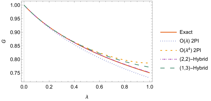
Figure 13: Comparison of exact $\bar{G}$, first and fourth order 2PI and$\left(2,2\right)$- and $\left(1,3\right)$-2PI-Padé hybrid solutions at small coupling. The $\left(2,2\right)$-hybrid solution lies almost on top of the exact solution.

Figure 14: Comparison of exact $\bar{G}$, first and fourth order 2PI and$\left(2,2\right)$- and $\left(1,3\right)$-2PI-Padé hybrid solutions at large coupling.

Now we try Padé summing the equation of motion:

$$G^{-1}=m^{2}+2\frac{G^{-1}\sum_{n=1}^{N}A_{n}^{\left(\partial\gamma\right)}\left(\lambda G^{2}\right)^{n}}{\sum_{n=0}^{M}B_{n}^{\left(\partial\gamma\right)}\left(\lambda G^{2}\right)^{n}},$$ (59)

where the explicit factor of $G^{-1}$ on the right hand side simply ensures the self-energy is an odd function of $G$ as it must be. This equation of motion is of degree $\max\left(2N,2M+1\right)$, which for typical choices of $N$ and $M$ results in a rough halving of the number of spurious solutions. To obtain an analytic result we consider the first non-trivial approximant, i.e. $N=M=1$. The resulting equation of motion is

$$G^{-1}=m^{2}+\frac{1}{2}\frac{\lambda G}{1+\frac{1}{3}\lambda G^{2}},$$ (60)

which agrees with the usual 2PI equation of motion up to terms of order $\mathcal{O}\left(\lambda^{3}\right)$, however it only has two spurious solutions instead of three. The physical solution obtained by matching at small $\lambda$ is

$$G_{\text{hy}}=\frac{1}{6m^{2}}\left(-1+\frac{36m^{4}-\lambda}{X^{1/3}}-\frac{X^{1/3}}{\lambda}\right),$$ (61)

where

$$X=\lambda^{3}-378\lambda^{2}m^{4}+18\lambda m^{2}\sqrt{\lambda\left(-2\lambda^{2}+144m^{8}+429\lambda m^{4}\right)}.$$

Indeed, this matches perturbation theory up to $\mathcal{O}\left(\lambda^{3}\right)$ terms. However, the large $\lambda$ behaviour in this approximation is pathological:

$$G_{\text{hy}}\to-\frac{1}{2m^{2}}+\frac{18m^{2}}{\lambda}+\mathcal{O}\left(\lambda^{-3/2}\right),$$ (62)

as $\lambda\to\infty$. This reflects the existence of an unphysical branch cut on the positive $\lambda$ axis starting at $\lambda/m^{4}=\frac{3}{4}\left(143+19\sqrt{57}\right)\approx 214$, which $G_{\text{hy}}$ has in addition to the expected cuts on the negative axis. The existence of this cut also renders the derivation of the spectral function invalid, meaning that $G_{\text{hy}}$ cannot be written in the form (14). It is not clear at this stage whether other forms of Padé summed equations of motion lack these pathologies. We leave further investigation of hybrid approximation schemes to future work.

6 Discussion

Two-particle irreducible effective actions are the subject of a rich literature and have found applications in diverse areas from early universe cosmology to nano-electronics (e.g. [23, 24]). The virtues of approximation schemes built on 2PI effective actions are often explained in terms of a resummation of an infinite series of perturbative Feynman diagrams which are encapsulated in the non-perturbative Green function $G$, from which the 2PI diagram series is built. However, the 2PI effective action is not a resummation scheme: it is a self-consistent variational principle. The definition of the 2PI effective action in terms of the Legendre transform is crucial for the self-consistency of the scheme. The immediate practical consequence is that any modification of the 2PI effective action which does not derive from a consistent modified variational principle is very likely to be inconsistent. So for instance, the consistency of recent attempts to improve the symmetry properties of 2PI effective actions [25] is guaranteed by the existence of a suitable constrained variational principle, however, ad hoc attempts to modify the equations of motion to satisfy symmetries will fail.

In this work we have pointed out the distinction between resummation and self-consistent approximations using an exactly solvable zero dimensional “field” theory. The perturbation theory has zero radius of convergence due to a branch cut on the negative coupling ($\lambda$) axis, a fact which is invisible to perturbation theory. The theory is Borel summable, with the Borel sum giving the exact answer. However, Borel summation alone is not usually this helpful in practice. Padé approximants well describe the Green function at weak coupling, though not at strong coupling. However, the combination of Borel and Padé approximation yields an effective global approximation scheme for the Green function.

The two point Green function of this theory admits a nice integral representation in terms of the spectral function (i.e. discontinuity of the branch cut) which allows us to see that the Padé approximants improve perturbation theory by allowing the spectral function to be approximated as a sum of delta functions and the Borel-Padé method gives a continuous, albeit erratic and inaccurate, approximation to the spectral function.

The 2PI approximation scheme surpasses perturbation theory, Padé and Borel-Padé approximants already at the leading non-trivial truncation. Like the Borel-Padé method, 2PI approximations can develop branch points and represent the spectral function by a continuous distribution. However, the 2PI approximation is quantitatively superior at the leading truncation.

We speculate that this is because the Borel-Padé method is a widely applicable general “black box” method, however the self-consistent 2PI equations of motion are derived within a particular field theory of interest. This gives the 2PI method “insider information,” from which it should be able to construct a better approximation. This comes at the cost of spurious solutions which must be eliminated and the added difficulty of finding the 2PI effective action in the first place.

Finally we introduced (for the first time, to our knowledge) a hybrid 2PI-Padé scheme, using Padé approximants to partially resum the 2PI diagram series. The quality of the result depends strongly on the type of Padé approximant used, with the best result in our case for the diagonal approximant. This hybrid approximation performs considerably better than the comparable 2PI approximation at weak coupling, though not noticeably better at strong coupling.

During proofing we became aware of a work by Kleinert [26] in some ways similar to our own. In [26], Kleinert generalizes and reformulates the Feynman-Kleinert variational perturbation theory and compares it to the 2PI effective action (called by the non-standard name “bilocal Legendre transform”) for the toy model discussed here. He finds that the variational perturbation theory out-performs the 2PI method and notes especially the failure of the 2PI series to converge uniformly for all couplings (this is not a surprise in light of the fact that the 2PI series is asymptotic). Our work differs in scope from his in two major ways. First, we compare the 2PI method to traditional resummation methods and not to other variational methods. Second, Kleinert focuses on the value of the effective action itself evaluated at its extremum, while we focus on the correlation function. In particular, we have focused on the analytic structure of the correlation function in the complex coupling plane, and introduced the spectral representation to aid this discussion. A study of the behaviour of these quantities in variational perturbation theory is an intriguing prospect for future work. (An intermediate result of Kleinert’s work is directly applicable to our discussion around (47): equation 110 of [26] gives a non-linear recurrence relation for the coefficients of the 2PI self-energy.)

There are several other natural directions for extension of this work. One would be the calculation and comparison of higher orders in the 2PI and (Borel-)Padé approximations, although it is doubtful what new insights might come from this. It would be straightforward to extend this work to consider 4PI effective actions, which depend on a self-consistent vertex function $V^{\left(4\right)}$ in addition to $G$. However, the extension to higher order $n$PI effective actions requires the introduction of new terms in the exponent of (1) which makes the problem no longer exactly solvable. A natural direction to pursue is Borel-Padé summation of the 2PI generating functional itself. This opens the possibility of eliminating spurious solutions to the 2PI equations of motion and enhancing the sensitivity of the 2PI method to the exponentially small regions of the spectral function, hence eliminating unphysical cusps. We are planning an investigation of these themes for the quantum anharmonic oscillator as a stepping stone to more physically interesting field theories.

References

-
[1]
T. D. Lee, C. N. Yang,
Many-Body Problem
in Quantum Statistical Mechanics. IV. Formulation in Terms of
Average Occupation Number in Momentum Space, Physical Review
117 (1) (1960) 22–36.
doi:10.1103/PhysRev.117.22.
URL http://link.aps.org/doi/10.1103/PhysRev.117.22 -
[2]
J. M. Luttinger, J. C. Ward,
Ground-State
Energy of a Many-Fermion System. II, Physical Review 118 (5)
(1960) 1417–1427.
doi:10.1103/PhysRev.118.1417.
URL http://link.aps.org/doi/10.1103/PhysRev.118.1417 -
[3]
G. Baym,
Self-consistent
approximations in many-body systems, Phys. Rev. 127 (1962) 1391–1401.
doi:10.1103/PhysRev.127.1391.
URL http://link.aps.org/doi/10.1103/PhysRev.127.1391 -
[4]
J. Cornwall, R. Jackiw, E. Tomboulis,
Effective action for
composite operators, Phys. Rev. D 10 (8) (1974) 2428–2445.
doi:10.1103/PhysRevD.10.2428.
URL http://link.aps.org/doi/10.1103/PhysRevD.10.2428 -
[5]
J. Berges,
Introduction
to nonequilibrium quantum field theory, AIP Conf. Proc. 739 (1) (2004)
3–62.
arXiv:hep-ph/0409233, doi:http://dx.doi.org/10.1063/1.1843591.
URL http://scitation.aip.org/content/aip/proceeding/aipcp/10.1063/1.1843591 -
[6]
J. Berges, S. Borsányi,
Range of validity
of transport equations, Phys. Rev. D 74 (4) (2006) 045022.
arXiv:hep-ph/0512155, doi:10.1103/PhysRevD.74.045022.
URL http://link.aps.org/doi/10.1103/PhysRevD.74.045022 -
[7]
T. Arai, Effective
potential and Goldstone bosons in de Sitter space, Phys. Rev. D 88 (6)
(2013) 064029.
arXiv:1304.5631,
doi:10.1103/PhysRevD.88.064029.
URL http://link.aps.org/doi/10.1103/PhysRevD.88.064029 -
[8]
A. Pilaftsis, D. Teresi, Symmetry
Improved 2PI Effective Action and the Infrared Divergences of the Standard
Model. arXiv:1502.07986.
URL http://arxiv.org/abs/1502.07986 - [9] C. M. Bender, T. T. Wu, Large-order behavior of perturbation theory, Phys. Rev. Lett. 27 (7) (1971) 461–465. doi:10.1103/PhysRevLett.27.461.
- [10] C. M. Bender, Perturbation theory in large order, Advances in Mathematics 30 (3) (1978) 250–267. doi:10.1016/0001-8708(78)90039-7.
-
[11]
S. Coleman, Fate of the
false vacuum: Semiclassical theory, Phys. Rev. D 15 (1977) 2929–2936.
doi:10.1103/PhysRevD.15.2929.
URL http://link.aps.org/doi/10.1103/PhysRevD.15.2929 - [12] F. J. Dyson, Divergence of perturbation theory in quantum electrodynamics, Phys. Rev. 85 (4) (1952) 631–632. doi:10.1103/PhysRev.85.631.
-
[13]
M. Beneke, P. Moch,
On “dynamical
mass” generation in Euclidean de Sitter space, Phys. Rev. D 87 (2013)
064018.
arXiv:1212.3058,
doi:10.1103/PhysRevD.87.064018.
URL http://link.aps.org/doi/10.1103/PhysRevD.87.064018 -
[14]
A. Malbouisson, R. Portugal, N. Svaiter,
A
Non-perturbative Solution of the Zero-Dimensional lambda phi^4 Field
Theory, Physica A 292 (1-4) (1999) 11.
arXiv:hep-th/9909175, doi:10.1016/S0378-4371(00)00587-2.
URL http://www.sciencedirect.com/science/article/pii/S0378437100005872 - [15] W. Y. Crutchfield, Method for Borel-summing instanton singularities: Introduction, Phys. Rev. D 19 (8) (1979) 2370–2384. doi:10.1103/PhysRevD.19.2370.
-
[16]
C. M. Bender, S. A. Orszag,
Advanced
Mathematical Methods for Scientists and Engineers I, Springer-Verlag, New
York, 1999.
URL https://www.springer.com/mathematics/analysis/book/978-0-387-98931-0 - [17] J. Ellis, E. Gardi, M. Karliner, M. A. Samuel, Padé approximants, Borel transforms and renormalons: The Bjorken sum rule as a case study, Phys. Lett. B 366 (1-4) (1996) 268–275. arXiv:hep-ph/9509312, doi:10.1016/0370-2693(95)01326-1.
-
[18]
D. Dorigoni, An Introduction to
Resurgence, Trans-Series and Alien Calculus. arXiv:1411.3585.
URL http://arxiv.org/abs/1411.3585 -
[19]
M. Beneke,
Renormalons,
Physics Reports 317 (1-2) (1999) 1–142.
doi:10.1016/S0370-1573(98)00130-6.
URL http://linkinghub.elsevier.com/retrieve/pii/S0370157398001306 -
[20]
G. V. Dunne, M. Ünsal,
Uniform WKB,
multi-instantons, and resurgent trans-series, Physical Review D 89 (10).
doi:10.1103/PhysRevD.89.105009.
URL http://link.aps.org/doi/10.1103/PhysRevD.89.105009 -
[21]
G. Basar, G. V. Dunne, M. Ünsal,
Resurgence theory,
ghost-instantons, and analytic continuation of path integrals, Journal of
High Energy Physics 2013 (10).
arXiv:1308.1108,
doi:10.1007/JHEP10(2013)041.
URL http://link.springer.com/10.1007/JHEP10(2013)041 -
[22]
U. Kraemmer, A. Rebhan, Advances in
perturbative thermal field theory, Rep. Prog. Phys. 67 (3) (2004) 351–431.
arXiv:hep-ph/0310337, doi:10.1088/0034-4885/67/3/R05.
URL http://arxiv.org/abs/hep-ph/0310337 -
[23]
J. Berges, Nonequilibrium Quantum
Fields : From Cold Atoms to Cosmology. arXiv:1503.02907v1.
URL http://arxiv.org/abs/1503.02907v1 -
[24]
E. Calzetta, B.-L. Hu, Nonequilibrium
Quantum Field Theory, Cambridge University Press, Cambridge, 2008.
URL www.cambridge.org/9780521641685 -
[25]
A. Pilaftsis, D. Teresi,
Symmetry
Improved CJT Effective Action, Nucl. Phys. B 874 (2) (2013) 31.
arXiv:1305.3221,
doi:10.1016/j.nuclphysb.2013.06.004.
URL http://linkinghub.elsevier.com/retrieve/pii/S0550321313003180 -
[26]
H. Kleinert,
Systematic
Improvement of Hartree-Fock-Bogoliubov Approximation with
Exponentially Fast Convergence from Variational Perturbation
Theory, Annals of Physics 266 (1) (1998) 135–161.
doi:10.1006/aphy.1998.5789.
URL http://linkinghub.elsevier.com/retrieve/pii/S000349169895789X