Iterated quasi-reversibility method applied to elliptic and parabolic data completion problems

Abstract.

We study the iterated quasi-reversibility method to regularize ill-posed elliptic and parabolic problems: data completion problems for Poisson’s and heat equations. We define an abstract setting to treat both equations at once. We demonstrate the convergence of the regularized solution to the exact one, and propose a strategy to deal with noise on the data. We present numerical experiments for both problems: a two-dimensional corrosion detection problem and the one-dimensional heat equation with lateral data. In both cases, the method prove to be efficient even with highly corrupted data.

Jérémi Dardé

Institut de Mathématiques de Toulouse ; UMR5219

Université de Toulouse ; CNRS

UPS IMT, F-31062 Toulouse Cedex 9, France.

1. Introduction

We consider data completion problems for elliptic and parabolic operators. We start with elliptic operators: we consider a bounded domain $\Omega\subset\mathbb{R}^{d}$, $d\geq 2$, with Lipschitz boundary (see [3]). Let $\nu\in L^{\infty}(\partial\Omega,\mathbb{R}^{d})$ be the exterior unit normal of $\partial\Omega$, and $\Gamma,\ \Gamma_{c}\subset\partial\Omega$, such that $\partial\Omega=\overline{\Gamma\cup\Gamma_{c}}$ and $meas(\Gamma),\ meas(\Gamma_{c})>0$. Let $\sigma:\Omega\mapsto\mathbb{R}^{d\times d}$ be a real matrix valued function such that $\sigma\in W^{1,\infty}(\Omega)^{d\times d}$ and

$$\sigma=\sigma^{T},\quad c\,|\xi|^{2}\leq\sigma\xi\cdot\xi,\ \forall\xi\in\mathbb{R}^{d},\ \textit{a.e. in }\Omega.$$

The data completion problem is:

Problem.

For $f$, $g_{D}$ and $g_{N}$ in $L^{2}(\Omega)\times L^{2}(\Gamma)\times L^{2}(\Gamma)$, find $u\in H^{1}(\Omega)$ such that

$$\left\{\begin{array}[]{ccl}-\nabla\cdot\sigma\nabla u&=&f\text{ in }\Omega\\ u&=&g_{D}\text{ on }\Gamma\\ \sigma\nabla u\cdot\nu&=&g_{N}\text{ on }\Gamma.\end{array}\right.$$

This problem is well-known to be ill-posed (see [1, 2] and the references therein): it does not necessarily admit a solution for any data $(f,g_{D},g_{N})$, and if a solution exists, it does not depend continuously on the data. On the other hand, if the problem admits a solution $u_{s}$, this solution is necessarily unique (see e.g. [1, 4]).

Such a problem is encountered in many practical applications, among others in plasma physic [5, 6], or corrosion detection problems [8, 9, 7, 11, 10]. We will be particularly interested in the corrosion detection problem: in this problem, $u$ is the electrical potential inside a conductive object $\Omega$, $\sigma$ is the conductivity of the object, $g_{N}$ represent a current imposed on $\Gamma$, accessible part of the boundary of $\Omega$, and $g_{D}$ is the corresponding potential measured on $\Gamma$. The aim is to determine if some portion of the inaccessible part of the boundary $\Gamma_{c}$ is corroded.

Mathematically, it exists a non-negative function $\mu$ define on $\Gamma_{c}$ such that

$$\sigma\nabla u\cdot\nu+\mu\,u=0\text{ on }\Gamma_{c}$$

and the objective is to reconstruct $\mu$: $\mu=0$ on the healthy part of $\Gamma_{c}$, and $\mu>0$ on the corroded part. In section 6.1, we test our method on this problem.

The data completion problem is known to be severely, even exponentially ill-posed [2]. Therefore ones needs to use regularization methods to try to reconstruct $u$. Several methods have been proposed to stabilize the problem: see, e.g., [12, 13, 14, 15, 16, 17] and the references therein.

We are also interesting in the data completion problem for the heat equation, which is quite similar to the elliptic one, except that this time $u$ solves a parabolic equation. Such inverse problem appears naturally in thermal imaging [33] and inverse obstacle problems [34, 35]. For $T>0$, we define $\mathcal{Q}:=(0,T)\times\Omega$. Let $f$ be in $L^{2}(\mathcal{Q})$, $g_{D}$ and $g_{N}$ in $L^{2}(0,T;L^{2}(\Gamma))$. The data completion problem is then

Problem.

find $u\in H^{1,1}(\mathcal{Q}):=L^{2}(0,T;H^{1}(\Omega))\cap H^{1}(0,T;L^{2}(\Omega))$ such that

$$\left\{\begin{array}[]{rcl}\partial_{t}u-\Delta u&=&f\text{ in }\mathcal{Q}\\ u&=&g_{D}\text{ on }(0,T)\times\Gamma\\ \nabla u\cdot\nu&=&g_{N}\text{ on }(0,T)\times\Gamma\end{array}\right.$$

This parabolic data completion problem is also severely ill-posed (see e.g. [18]). Note that it is not mandatory to impose an initial condition $u(0,.)$ on $\Omega$ to obtain the uniqueness of the solution (if such a solution exists). Again, regularization methods are needed to obtain a stable reconstruction of $u$ from the data $f,\,g_{D}$ and $g_{N}$.

The quasi-reversibility method is such a regularization method, introduced in the pioneering work of Lattès and Lions [19] to regularize elliptic, parabolic (and even hyperbolic) data completion problems. The mean idea of the method is to approach the ill-posed data completion problem by a family of well-posed variational problems of higher order (typically fourth order problems) depending on a (small) parameter $\varepsilon$. The solution of the regularized problem converges to the solution of the data completion problem, when the parameter $\varepsilon$ goes to zero. The quasi-reversibility method presents interesting features: first of all the variational problems appearing in the method are naturally discretized using finite element methods, thus the method can be used in complicated geometries, an interesting property when the method is used in an iterative algorithm with changing domain. Furthermore, the method is independent of the dimension. Since its introduction, the quasi-reversibility method has been successfully used to reconstruct the solution of elliptic [20, 21, 23, 24, 25] and parabolic [29, 30] ill-posed problems, and as a keystone in the resolution of inverse obstacle problems in the exterior approach [26, 27, 28].

In the present paper, we are interested in a natural extension of the quasi-reversibility method, the iterated quasi-reversibility method: it consists in solving iteratively quasi-reversibility problems, the solution of each one depending on the solution of the previous one. We therefore obtain a sequence of quasi-reversibility solutions, which converges to the exact solution of the data completion problem if exact data are provided, for any choice of the regularization parameter $\varepsilon$. This has interesting consequences from a numerical point of view: first of all, one can now choose a large value for the parameter of regularization $\varepsilon$, leading to an improvement in the conditioning of the finite-element problems, without lowering the quality of the reconstruction. This is not the case for the standard quasi-reversibility method, for which it is mandatory to use small $\varepsilon$ to obtain a good reconstruction. Furthermore, in presence of noisy data, we present a method to choose when to stop the iterations according to the amplitude of noise on the data, based on the Morozov discrepancy principle, which ensure both stability and convergence of the method. The main drawback of this extension of the quasi-reversibility method, comparatively to the standard quasi-reversibility, is that several problems have to be solved to obtain a good reconstruction. However, as it is the same variational problem that appears in each iteration of the method, one can precompute a factorization of the finite-element matrix. Hence, the cost of the method is not significantly higher.

The paper is organized as follows. In section 2, we introduce an abstract setting to treat both data completion problems we are interested in at once. In section 3, we present the standard quasi-reversibility regularization in this abstract setting, and prove some results we need to study the iterated quasi-reversibility method. In section 4, we focus on the iterated quasi-reversibility method, both in the case of exact data and noisy data. In section 5, we show that the abstract setting apply to both elliptic and parabolic data completion problems. In section 6, numerical results are presented, demonstrating the feasibility and efficiency of the method for both problems.

2. An abstract setting for data completion problems

In this section, we set up an abstract setting corresponding to both data completion problems we are interested in.

Let $\mathcal{X}$, $\mathcal{Y}$ be two Hilbert spaces endowed with respective scalar products $(.,.)_{\mathcal{X}}$ and $(.,.)_{\mathcal{Y}}$, and corresponding norms denoted $\|.\|_{\mathcal{X}}$ and $\|.\|_{\mathcal{Y}}$.

Let $y\in\mathcal{Y}$. Both of our data completion problems can be written in the following way: find $x\in\mathcal{X}$ such that $Ax=y$, with $A:\mathcal{X}\mapsto\mathcal{Y}$ a continuous linear operator with following properties:

• $A$ is one-to-one

• $A$ is not onto

• $\overline{\mathsf{Im}(A)}^{\mathcal{Y}}=\mathcal{Y}$.

In this setting, $y$ plays the role of the data, and $x$ the solution of our data completion problem. The problem is obviously ill-posed: indeed, as $A$ is not onto, there exist $y$ in $\mathcal{Y}$ for which the problem admits no solution. We define $\mathcal{Y}_{adm}:=\mathsf{Im}(A)$ the set of admissible data, and $\mathcal{Y}_{nadm}=\mathcal{Y}\setminus\mathcal{Y}_{adm}$ the set of non-admissible ones. By definition, $\mathcal{Y}_{adm}$ is dense in $\mathcal{Y}$. Actually, this is also true for $\mathcal{Y}_{nadm}$

Proposition 1.

The set $\mathcal{Y}_{nadm}$ is dense in $\mathcal{Y}$.

Proof.

This is quite simple: suppose it exists $\bar{y}\in\mathcal{Y}_{adm}$ and $\delta>0$ such that $\|y-\bar{y}\|_{\mathcal{Y}}\leq\delta\Rightarrow y\in\mathcal{Y}_{adm}.$ It exists $\bar{x}\in\mathcal{X}$ s.t. $A\bar{x}=\bar{y}$.

Let $y$ be any element of $\mathcal{Y}$, $y\neq\bar{y}$. We define $\tilde{y}=\displaystyle\frac{y-\bar{y}}{\|y-\bar{y}\|_{\mathcal{Y}}}\frac{\delta}{2}+\bar{y}$. Obviously, $\|\tilde{y}-\bar{y}\|_{\mathcal{Y}}\leq\delta$. Therefore, $\tilde{y}\in\mathcal{Y}_{adm}$, and it exists $\tilde{x}\in\mathcal{X}$ such that $A\tilde{x}=\tilde{y}$. A simple computation shows then that

$$A\Big{(}\frac{2\|y-\bar{y}\|_{\mathcal{Y}}}{\delta}(\tilde{x}-\bar{x})+\bar{x}\Big{)}=y.$$

Hence $Im(A)=\mathcal{Y}$, contradicting the assumptions on $A$. Therefore, for any $y\in\mathcal{Y}_{adm}$, for any $\delta>0$, there exists $y^{\delta}\in\mathcal{Y}_{nadm}$ such that $\|y-y^{\delta}\|_{\mathcal{Y}}\leq\delta$, which ends the proof, as $\mathcal{Y}=\mathcal{Y}_{adm}\cup\mathcal{Y}_{nadm}$. ∎

In other word, for any admissible data $y$ exists a non-admissible one $\tilde{y}$ arbitrary close to $y$. In particular, this leads to the high instability of the problem with respect to noise:

Proposition 2.

For any $y\in\mathcal{Y}$, the exists a sequence $x_{n}\in\mathcal{X}$ such that

$$\|x_{n}\|_{\mathcal{X}}\xrightarrow[]{n\rightarrow\infty}+\infty\text{ and }Ax_{n}\xrightarrow[\mathcal{Y}]{n\rightarrow\infty}y.$$

Proof.

We start with $y\in\mathcal{Y}_{nadm}$. As $\textsf{Im}(A)$ is dense in $\mathcal{Y}$, it exists a sequence $x_{n}\in\mathcal{X}$ in such that $Ax_{n}\xrightarrow[\mathcal{Y}]{n\rightarrow\infty}y$. This sequence cannot have any bounded subsequence: indeed, if such a subsequence would exist, there would be another subsequence, denoted $x_{m}$ here, such that $x_{m}$ weakly converges to an element $x$ in $\mathcal{X}$. The operator $A$ being linear and strongly continuous, it is weakly continuous [38], hence $Ax_{m}$ weakly converges to $Ax$. But by definition $Ax_{m}$ strongly converges to $y$. By uniqueness of the limit, we have $Ax=y$, and $y\in\mathcal{Y}_{adm}$, in contradiction with the initial assumption. Therefore, we have $\|x_{n}\|_{\mathcal{X}}\xrightarrow[]{n\rightarrow\infty}+\infty$.

Now, consider $y\in\mathcal{Y}_{adm}$. The previous proposition implies the existence of a sequence $y_{m}\in\mathcal{Y}_{nadm}$ such that $y_{m}\xrightarrow[\mathcal{Y}]{m\rightarrow\infty}y$. For a fixed $m$, we now know the existence of a sequence $x_{m,n}\in\mathcal{X}$ such that $Ax_{m,n}\xrightarrow[\mathcal{Y}]{n\rightarrow\infty}y_{m}$ and $\|x_{m,n}\|_{\mathcal{X}}\xrightarrow[]{n\rightarrow\infty}+\infty$. In particular, for any $m\in\mathbb{N}$, there exists $n(m)\in\mathbb{N}$ such that $\tilde{x}_{m}:=x_{m,n(m)}$ verifies at the same time

$$\|\tilde{x}_{m}\|_{\mathcal{X}}\geq m\text{ and }\|A\tilde{x}_{m}-y_{m}\|_{\mathcal{Y}}\leq\frac{1}{m}.$$

It is then not difficult to verify that the sequence $\tilde{x}_{m}$ verifies the researched properties. ∎

Remark 1.

Actually, if $y$ is not an admissible data, it is shown in the proof that any sequence $(x_{n})_{n\in\mathbb{N}}\in\mathcal{X}^{\mathbb{N}}$ such that $Ax_{n}\xrightarrow[\mathcal{Y}]{n\rightarrow\infty}y$ verifies $\displaystyle\lim_{n\rightarrow\infty}\|x_{n}\|_{\mathcal{X}}=+\infty$.

This proposition has for important consequences the fact that for any admissible data $y$, with corresponding solution $x$, one can find an admissible data $\tilde{y}$, with corresponding solution $\tilde{x}$, such that $\tilde{y}$ is arbitrarily close to $y$ and $\tilde{x}$ is arbitrarily far from $x$.

We retrieve here the well-known fact that the problem of noisy data is crucial in data completion problems. Clearly, it is not sufficient to build a method that (approximately) reconstruct the solution of the data completion problem for any admissible data, it is also mandatory to propose a strategy for noisy data, as in practice data are always corrupted by some noise due to inaccurate measurements.

3. Standard quasi-reversibility method

We define $b$ a symmetric bilinear non-negative form on $\mathcal{X}$, and denote by $\|.\|_{b}$ the induced seminorm on $\mathcal{X}$. We suppose that it exists two strictly positive constants $c,\ C$ such that

$$c^{2}\|x\|_{\mathcal{X}}^{2}\leq\|Ax\|_{\mathcal{Y}}^{2}+\|x\|_{b}^{2}\leq C^{2}\|x\|_{\mathcal{X}}^{2}.$$

Therefore, the symmetric bilinear form $(.,.)_{A,b}$, define by

$$\forall(x,\tilde{x})\in\mathcal{X},(x,\tilde{x})_{A,b}=(Ax,A\tilde{x})_{Y}+b(x,\tilde{x}),$$

is a scalar product on $\mathcal{X}$, and $\mathcal{X}$ endowed with this scalar product is a Hilbert space. We denote $\|.\|_{A,b}$ the corresponding norm, which is equivalent to the $\|.\|_{\mathcal{X}}$ norm.

Obviously, there exists such a form $b$: it suffices to take the whole scalar product in $\mathcal{X}$, $b(.,.)=(.,.)_{\mathcal{X}}$.

Adapting the initial idea of Jacques-Louis Lions and Robert Lattès [19], the quasi-reversibility method applied to the abstract data completion problem defined above relies on the resolution of the following regularized problem

Problem.

for $y\in\mathcal{Y}$ and $\varepsilon>0$, find $x_{\varepsilon}\in\mathcal{X}$ such that

$$(Ax_{\varepsilon},Ax)_{\mathcal{Y}}+\varepsilon\,b(x_{\varepsilon},x)=(y,Ax)_{\mathcal{Y}},\quad\forall x\in\mathcal{X}.$$

The quasi-reversibility equation is the Euler-Lagrange equation corresponding to the minimization over $\mathcal{X}$ of the energy $\|Ax-f\|_{\mathcal{Y}}^{2}+\varepsilon\|x\|_{b}^{2}$. In other words, it is a Tykhonov regularization of the data completion problem, $\varepsilon>0$ being the parameter of regularization and $\|.\|_{b}$ the penalization (semi)norm. Since its introduction in 1963 by A.N. Tykhonov [37], this regularization has been widely studied and used to solve inverse problems (for a complete study on the topic, see [36] and the references therein). There are various methods to study such regularization method: e.g. singular value decomposition if $A$ is compact (which is not the case in our data completion problems, see section 5) or spectral theory. Here we propose another approach to study the method, based on the variational formulation of the quasi-reversibility method, and on the differentiability of the approximated solution with respect to the parameter of regularization, the later being useful in the study of the iterated quasi-reversibility method.

First of all, let us verify that the quasi-reversibility problem is well-posed.

Proposition 3.

For any $y\in\mathcal{Y}$ and $\varepsilon>0$, the quasi-reversibility problems admits a unique solution $x_{\varepsilon}$, with the following estimates:

$$\|Ax_{\varepsilon}\|_{\mathcal{Y}}\leq\|f\|_{\mathcal{Y}},\quad\|Ax_{\varepsilon}-y\|_{\mathcal{Y}}\leq\|y\|_{\mathcal{Y}},\quad\|x_{\varepsilon}\|_{A,b}\leq\frac{1}{\min(1,\sqrt{\varepsilon})}\|y\|_{\mathcal{Y}}.$$

Proof.

let us define the bilinear form

$$a_{\varepsilon}(x,\tilde{x}):=(Ax,A\tilde{x})_{\mathcal{Y}}+\varepsilon\ b(x,\tilde{x}),\quad\forall x,\ \tilde{x}\in\mathcal{X}.$$

It is obviously continuous. Furthermore, for all $x\in X$, we have

$$a_{\varepsilon}(x,\tilde{x})\geq\min(1,\varepsilon)\|x\|_{A,b}^{2},$$

and therefore it is coercive. Finally, as $|(y,Ax)_{\mathcal{Y}}|\leq\|A\|\,\|y\|_{\mathcal{Y}}\,\|x\|_{\mathcal{X}}\leq\|A\|\,\|y\|_{\mathcal{Y}}\,\|x\|_{A,b}$, we obtain the existence and uniqueness of $x_{\varepsilon}$ by Lax-Milgram theorem. By definition, we have

$$\|Ax_{\varepsilon}\|_{\mathcal{Y}}^{2}\leq\|Ax_{\varepsilon}\|_{\mathcal{Y}}^{2}+\varepsilon\|x_{\varepsilon}\|_{b}^{2}=(Ax_{\varepsilon},y)_{\mathcal{Y}}\leq\|Ax_{\varepsilon}\|_{\mathcal{Y}}\|y\|_{\mathcal{Y}}\Rightarrow\|Ax_{\varepsilon}\|_{\mathcal{Y}}\leq\|y\|_{\mathcal{Y}}.$$

Furthermore,

$$(Ax_{\varepsilon}-y,Ax_{\varepsilon})_{\mathcal{Y}}=-\varepsilon\|x_{\varepsilon}\|_{b}^{2}\leq 0\Rightarrow\|Ax_{\varepsilon}-y\|_{\mathcal{Y}}^{2}\leq-(y,Ax_{\varepsilon}-y)_{\mathcal{Y}}\leq\|y\|_{Y}\|Ax_{\varepsilon}-y\|_{\mathcal{Y}},$$

implying $\|Ax_{\varepsilon}-y\|_{\mathcal{Y}}\leq\|y\|_{\mathcal{Y}}$. Finally, we have

$$\|Ax_{\varepsilon}\|_{\mathcal{Y}}^{2}+\varepsilon\|x_{\varepsilon}\|_{b}^{2}=(Ax_{\varepsilon},y)_{\mathcal{Y}}\leq\|Ax_{\varepsilon}\|_{\mathcal{Y}}\|y\|_{\mathcal{Y}}\leq\sqrt{\|Ax_{\varepsilon}\|_{\mathcal{Y}}^{2}+\varepsilon\|x_{\varepsilon}\|_{b}^{2}}\,\|y\|_{\mathcal{Y}}$$

leading to $\displaystyle\min(1,\sqrt{\varepsilon})\|x_{\varepsilon}\|_{A,b}\leq\sqrt{\|Ax_{\varepsilon}\|_{\mathcal{Y}}^{2}+\varepsilon\|x_{\varepsilon}\|_{b}^{2}}\leq\|y\|_{Y}.$ ∎

Remark 2.

In particular, we always have $x_{\varepsilon}\xrightarrow[\varepsilon\rightarrow\infty]{\mathcal{X}}0$.

Suppose there exists $x\in\mathcal{X}$ such that $Ax=y$ (i.e. $y\in\mathcal{Y}_{adm}$). It is easily seen that $x$ is never the solution of the quasi-reversibility problem, except in the special case $y=0$ (which is always in $\mathcal{Y}_{adm}$) for which $x=0=x_{\varepsilon}$. In other words, there is no $\varepsilon>0$ such that the quasi-reversibility method reconstructs exactly the exact solution of the data completion problem. As seen in the following corollary, the solution of the quasi-reversibility problem is also never $0$, except again in the special case $y=0$.

Corollary 1.

The three following properties are equivalent:

• $y\neq 0$

• $\exists\ \varepsilon>0$ s.t. $x_{\varepsilon}\neq 0$

• $\forall\varepsilon>0$, $x_{\varepsilon}\neq 0$.

Proof.

obviously, (iii) implies (ii). Furthermore, as $\min(1,\sqrt{\varepsilon})\|x_{\varepsilon}\|_{A,b}\leq\|y\|_{Y}$, (ii) implies (i).

Suppose it exists $\varepsilon>0$ such that $x_{\varepsilon}=0$. For that particular $\varepsilon$ and for any $x\in X$, we would have $(y,Ax)_{\mathcal{Y}}=(Ax_{\varepsilon},Ax)_{\mathcal{Y}}+\varepsilon(x_{\varepsilon},x)_{b}=0.$ As $\overline{Im(A)}^{\mathcal{Y}}=\mathcal{Y}$, this directly implies $y=0$, so (i) implies (iii). ∎

Proposition 4.

Let $y\in\mathcal{Y}$, and $x_{\varepsilon}$ the solution of the corresponding quasi-reversibility problem. Then $Ax_{\varepsilon}$ strongly converges to $y$ (even if $y$ is not an admissible data).

Proof.

As $\displaystyle\min(1,\sqrt{\varepsilon})\|x_{\varepsilon}\|_{A,b}\leq\|y\|_{\mathcal{Y}}$, we have, for any $x\in\mathcal{X}$,

$$\varepsilon|\,b(x_{\varepsilon},x)|\leq\frac{\varepsilon}{\min(1,\sqrt{\varepsilon})}\|y\|_{\mathcal{Y}}\|x\|_{b}\xrightarrow[]{\varepsilon\rightarrow 0}0.$$

Let $(\varepsilon_{m})_{m\in\mathbb{N}}$ be a decreasing sequence of strictly positive real numbers such that $\lim_{m\rightarrow\infty}\varepsilon_{m}=0$, and note $x_{m}:=x_{\varepsilon_{m}}$. As $\|Ax_{m}\|_{\mathcal{Y}}\leq\|y\|_{\mathcal{Y}}$, it exists a subsequence (still denoted $x_{m}$) such that $Ax_{m}$ weakly converges to $\tilde{y}\in\mathcal{Y}$. But, for all $x\in\mathcal{X}$, we have

$$(y-\tilde{y},Ax)_{\mathcal{Y}}\xleftarrow[]{m\rightarrow\infty}(y-Ax_{m},Ax)_{\mathcal{Y}}=\varepsilon_{m}b(x_{m},x)\xrightarrow[]{m\rightarrow\infty}0,$$

that is $y=\tilde{y}$ as $\overline{\mathsf{Im}(A)}^{\mathcal{Y}}=\mathcal{Y}$, and $Ax_{m}$ weakly converges to $y$. As $\|Ax_{m}\|_{\mathcal{Y}}\leq\|y\|_{\mathcal{Y}}$ (proposition 3), $Ax_{m}$ strongly converges to $y$. It is then not difficult to see that $Ax_{\varepsilon}$ strongly converges to $y$ as $\varepsilon$ goes to zero. ∎

We can now state the main theorem regarding the standard quasi-reversibility method:

Theorem 3.1.

Suppose $y\in\mathcal{Y}_{adm}$, and let $x_{s}$ be the (necessarily unique) solution of the abstract data completion problem. Then $x_{\varepsilon}$ converges to $x_{s}$ as $\varepsilon$ goes to zero, and we have the estimates $\|Ax_{\varepsilon}-y\|_{\mathcal{Y}}\leq\sqrt{\varepsilon}\|x_{s}\|_{b}$, $\|x_{\varepsilon}\|_{b}\leq\|x_{s}\|_{b}$ and $\|x_{\varepsilon}-x_{s}\|_{b}\leq\|x_{s}\|_{b}$.

Suppose $y\in\mathcal{Y}_{nadm}$. Then $\displaystyle\lim_{\varepsilon\rightarrow 0}\|x_{\varepsilon}\|_{b}=+\infty$.

The theorem remains valid when the $\|.\|_{b}$ seminorm is replaced with the $\|.\|_{A,b}$ norm.

Proof.

Suppose first that $y\in\mathcal{Y}_{nadm}$. Then, as $x_{\varepsilon}$ is a sequence in $\mathcal{X}$ such that $Ax_{\varepsilon}$ converges to $y$ (proposition 4), proposition 2 and remark 1 imply $\lim_{\varepsilon\rightarrow 0}\|x_{\varepsilon}\|_{\mathcal{X}}=+\infty$. As $\|x_{\varepsilon}\|_{A,b}^{2}=\|Ax_{\varepsilon}\|_{\mathcal{Y}}^{2}+\|x_{\varepsilon}\|_{b}^{2}\geq c^{2}\|x_{\varepsilon}\|_{\mathcal{X}}$, we have $\lim_{\varepsilon\rightarrow 0}\|x_{\varepsilon}\|_{b}=+\infty$.

Now, suppose it exists $x_{s}$ such that $Ax_{s}=y$. Then, choosing $x=x_{\varepsilon}-x_{s}$ as test function in the quasi-reversibility problem, we obtain

$$\|Ax_{\varepsilon}-y\|_{\mathcal{Y}}^{2}+\varepsilon b(x_{\varepsilon},x_{\varepsilon}-x_{s})=0,$$ (1)

which in turn implies $b(x_{\varepsilon},x_{\varepsilon}-x_{s})\leq 0\Rightarrow\|x_{\varepsilon}\|_{b}\leq\|x_{s}\|_{b}\Rightarrow\|x_{\varepsilon}\|_{A,b}\leq\|x_{s}\|_{A,b}$. Therefore, $x_{\varepsilon}$ is a bounded sequence in $\mathcal{X}$, and up to a subsequence it weakly converges to $\tilde{x}$. As $A$ is a linear continuous operator, and hence is weakly continuous, proposition 4 implies $A\tilde{x}=y$, which implies $\tilde{x}=x_{s}$ as $A$ is one-to-one. The uniqueness of the limit implies that the whole sequence weakly converges to $x_{s}$. Finally as $\|x_{\varepsilon}\|_{A,p}\leq\|x_{s}\|_{A,p}$, the sequence strongly converges to $x_{s}$.

Subtracting $\varepsilon b(x_{s},x_{\varepsilon}-x_{s})$ to equation 1, we obtain

$$\|Ax_{\varepsilon}-y\|_{\mathcal{Y}}^{2}+\varepsilon\|x_{s}-x_{\varepsilon}\|_{b}^{2}=-\varepsilon b(x_{s},x_{\varepsilon}-x_{s})\Rightarrow\|x_{s}-x_{\varepsilon}\|_{b}^{2}\leq|b(x_{s},x_{\varepsilon}-x_{s})|$$

and by Cauchy-Schwarz inequality, $\|x_{\varepsilon}-x_{s}\|_{b}\leq\|x_{s}\|_{b}$.

Finally, equation 1 implies

$$\|Ax_{\varepsilon}-y\|_{\mathcal{Y}}^{2}\leq\varepsilon\|x_{\varepsilon}\|_{b}\,\|x_{\varepsilon}-x_{s}\|_{b}\leq\varepsilon\|x_{s}\|^{2}_{b}$$

which ends the proof. ∎

Next, we focus on the differentiability of the solution of the quasi-reversibility method with respect to $\varepsilon$, a result that will be useful in the study of the iterated quasi-reversibility method.

3.1. Differentiability of the quasi-reversibility solution with respect to $\varepsilon$

It turns out that $x_{\varepsilon}$, solution of the quasi-reversibility problem, depends smoothly on the parameter of regularization $\varepsilon$. Indeed, let us define the map $F:\varepsilon>0\mapsto x_{\varepsilon}$.

Proposition 5.

The map $F$ is continuous.

Proof.

We choose $\varepsilon>0$ and $h$ such that $\varepsilon-|h|>0$. For any $x\in\mathcal{X}$, we have

$$(Ax_{\varepsilon+h},Ax)_{\mathcal{Y}} +(\varepsilon+h)\,b(x_{\varepsilon+h},x)=(y,Ax)_{\mathcal{Y}}$$

$$(Ax_{\varepsilon},Ax)_{\mathcal{Y}} +\varepsilon\ b(x_{\varepsilon},x)=(y,Ax)_{\mathcal{Y}}.$$

Subtracting the two equations, and choosing $x=\tilde{x}_{\varepsilon,h}:=x_{\varepsilon+h}-x_{\varepsilon}$, lead to

$$\|A\tilde{x}_{\varepsilon,h}\|_{\mathcal{Y}}^{2}+\varepsilon\,\|\tilde{x}_{\varepsilon,h}\|_{b}^{2}=-h\,b(x_{\varepsilon+h},\tilde{x}_{\varepsilon,h}).$$

In conclusion, we have

$$\min(1,\varepsilon)\,\|\tilde{x}_{\varepsilon,h}\|_{A,b}^{2}\leq h\|x_{\varepsilon+h}\|_{b}\|\tilde{x}_{\varepsilon,h}\|_{b}\leq h\min(1,(\varepsilon+h)^{-1/2})\|y\|_{\mathcal{Y}}\|\tilde{x}_{\varepsilon,h}\|_{A,b}$$

which ends the proof. ∎

Remark 3.

If the data completion problem admits a solution $x_{s}$, then $F$ extends continuously to $\mathbb{R}^{+}$ by defining $F(0)=x_{s}$.

Proposition 6.

We have $F\in C^{1}(\mathbb{R}^{+}_{*};\mathcal{X})$. For all $\varepsilon>0$, $F^{\prime}(\varepsilon)=x_{\varepsilon}^{(1)}$, unique element of $\mathcal{X}$ verifying

$$(Ax_{\varepsilon}^{(1)},Ax)_{\mathcal{Y}}+\varepsilon b(x_{\varepsilon}^{(1)},x)=-b(x_{\varepsilon},x),\quad\forall x\in\mathcal{X}.$$ (2)

Furthermore, $\|x_{\varepsilon}^{(1)}\|_{A,b}\leq\min(1,\varepsilon^{-\frac{3}{2}})\|y\|_{\mathcal{Y}}$.

Proof.

By Lax-Milgram theorem, there exists a unique $x_{\varepsilon}^{(1)}\in\mathcal{X}$ verifying 2, and it clearly verifies

$$\min(1,\varepsilon)\|x_{\varepsilon}^{(1)}\|_{A,b}^{2}\leq\|x_{\varepsilon}\|_{b}\|x_{\varepsilon}^{(1)}\|_{A,b}\leq\min(1,\varepsilon^{-\frac{1}{2}})\,\|y\|_{\mathcal{Y}}\|x_{\varepsilon}^{(1)}\|_{A,b}.$$

It is a continuous function of $\varepsilon$: indeed, for $\varepsilon>0$ and $h\in\mathbb{R}$ s.t. $\varepsilon-|h|>0$, we have, for all $x\in\mathcal{X}$,

$$(Ax_{\varepsilon+h}^{(1)},Ax)_{\mathcal{Y}}+(\varepsilon+h)\, b(x_{\varepsilon+h}^{(1)},x)=-b(x_{\varepsilon+h},x)$$

$$(Ax_{\varepsilon}^{(1)},Ax)_{\mathcal{Y}}+\varepsilon\ b(x_{\varepsilon}^{(1)},x)=-b(x_{\varepsilon},x).$$

Choosing $x=\tilde{x}_{\varepsilon,h}^{(1)}:=x_{\varepsilon+h}^{(1)}-x_{\varepsilon}^{(1)}\in\mathcal{X}$ and subtracting the two equations lead to

$$\|A\tilde{x}_{\varepsilon,h}^{(1)}\|_{\mathcal{Y}}^{2}+\varepsilon\|\tilde{x}_{\varepsilon,h}^{(1)}\|_{b}^{2}=-hb(x_{\varepsilon+h}^{(1)},\tilde{x}_{\varepsilon,h}^{(1)})-b(\tilde{x}_{\varepsilon,h},\tilde{x}_{\varepsilon,h}^{(1)}).$$

Therefore,

$$\|\tilde{x}_{\varepsilon,h}^{(1)}\|_{A,b}\leq h\Big{(}\min(1,(\varepsilon+h)^{-3/2})+\min(1,(\varepsilon+h)^{-1/2})\min(1,\varepsilon^{-1})\Big{)}\|y\|_{\mathcal{Y}}$$

implying the continuity of the map $\mathbb{R}^{+}_{*}\ni\varepsilon\mapsto x_{\varepsilon}^{(1)}\in\mathcal{X}$. Remains to be proved that $F^{\prime}(\varepsilon)=x_{\varepsilon}^{(1)}$. For $\varepsilon>0$ and $h\in\mathbb{R}$ such that $\varepsilon-|h|>0$, we have

$$(Ax_{\varepsilon+h},Ax)_{\mathcal{Y}} +(\varepsilon+h)\,b(x_{\varepsilon+h},x)=(y,Ax)_{\mathcal{Y}}$$

$$-(Ax_{\varepsilon},Ax)_{\mathcal{Y}} -\varepsilon\ b(x_{\varepsilon},x)=-(y,Ax)_{\mathcal{Y}}$$

$$-h\,(Ax_{\varepsilon}^{(1)},Ax)_{\mathcal{Y}} -h\,\varepsilon\ b(x_{\varepsilon}^{(1)},x)=h\,b(x_{\varepsilon},x).$$

Choosing $x=\hat{x}_{\varepsilon,h}:=x_{\varepsilon+h}-x_{\varepsilon}-hx_{\varepsilon}^{(1)}$ and adding the three above relations lead to

$$\|A\hat{x}_{\varepsilon,h}\|_{\mathcal{Y}}^{2}+\varepsilon\|\hat{x}_{\varepsilon,h}\|_{b}^{2}=-hb(\tilde{x}_{\varepsilon,h},\hat{x}_{\varepsilon,h})\Rightarrow\|\hat{x}_{\varepsilon,h}\|_{A,b}\leq h^{2}\ C(h,\varepsilon)\|y\|_{\mathcal{Y}},\text{ with }C(h,\varepsilon)>c>0.$$

The result follows. ∎

A simple induction leads then to the following theorem:

Theorem 3.2.

$F\in C^{\infty}(\mathbb{R}^{+}_{*};\mathcal{X})$. For $\varepsilon>0$, for all $m\in\mathbb{N}$,

$$\frac{d^{m}F}{d\varepsilon^{m}}(\varepsilon):=x^{(m)}_{\varepsilon}$$

with $x_{\varepsilon}^{(m)}$ defined recursively by

$$\left\{\begin{array}[]{l}x_{\varepsilon}^{(0)}:=x_{\varepsilon},\\ \forall m\in\mathbb{N},\ x_{\varepsilon}^{(m+1)}\text{ is the only element of }\mathcal{X}\text{ verifying }\\ (Ax_{\varepsilon}^{(m+1)},Ax)_{\mathcal{Y}}+\varepsilon\,b(x_{\varepsilon}^{(m+1)},x)=-(m+1)\,b(x_{\varepsilon}^{(m)},x),\ \forall x\in\mathcal{X}.\end{array}\right.$$

In particular, $x_{\varepsilon}^{(m)}$ verifies the following estimate:

$$\|x_{\varepsilon}^{(m)}\|_{A,b}\leq\frac{m\,!}{\min(1,\varepsilon^{m+1/2})}\|y\|_{\mathcal{Y}}.$$

If the data completion problem admits a solution $x_{s}$, it is not difficult to prove that

$$\|x_{\varepsilon}^{(m)}\|_{A,b}\leq\min(1,\varepsilon^{m})^{-1}\,m!\,\|x_{s}\|_{A,b}.$$

Finally, we have the following generalization of corollary 1:

Corollary 2.

the three following properties are equivalent:

• $y\neq 0$

• $\exists\varepsilon>0$, $\exists m\in\mathbb{N}$ s.t. $x_{\varepsilon}^{(m)}\neq 0$

• $\forall\varepsilon>0$, $\forall m\in\mathbb{N}$, $x_{\varepsilon}^{(m)}\neq 0$.

Proof.

Clearly (iii) implies (ii). Furthermore, as $\displaystyle\min(1,\varepsilon^{m+\frac{1}{2}})\,\|x_{\varepsilon}^{(m)}\|_{A,b}\leq m\,!\,\|y\|_{\mathcal{Y}}$, (ii) implies (i).

Suppose it exists $\varepsilon>0$ and $m\in\mathbb{N}$ such that $x_{\varepsilon}^{(m)}=0$. If $m=0$, then corollary 1 implies $y=0$. If $m>0$, as $(Ax_{\varepsilon}^{(m)},Ax_{\varepsilon}^{(m-1)})_{\mathcal{Y}}+\varepsilon\,b(x_{\varepsilon}^{(m)},x_{\varepsilon}^{(m-1)})=-m\|x_{\varepsilon}^{(m-1)}\|_{b}^{2}$, we obtain $x_{\varepsilon}^{(m-1)}=0$, and by induction $x_{\varepsilon}=0$, implying again $y=0$. Therefore (i) implies (iii). ∎

3.2. Monotonic convergence of the quasi-reversibility method

In this section, $y\neq 0$. Using the results on the derivatives of $x_{\varepsilon}$ with respect to $\varepsilon$, it is easy to prove that if the data completion problem admits a solution $x_{s}$, then $x_{\varepsilon}$ converges monotonically to $x_{s}$ when $\varepsilon$ goes to zero. This is of course not the only method to obtain such results (see for example [36], where spectral theory is used), but it has the advantage to be quite simple.

The main result of this section is the following

Theorem 3.3.

Suppose the data completion problem admits a unique solution $x_{s}$. Then $\|x_{\varepsilon}-x_{s}\|_{A,b}$ is strictly increasing with respect to $\varepsilon$.

We need to prove first the following two results, which are true whether or not the data completion problem admits a solution:

Lemma 3.4.

For all $m\in\mathbb{N}$, for all $n\in\mathbb{N}$, $\displaystyle(-1)^{m+n}b(x_{\varepsilon}^{(m)},x_{\varepsilon}^{(n)})>0$.

Proof.

For $m\in\mathbb{N}$, let us define the axiom of induction:

$$P(m):\quad\forall n\in\left\{0,\cdots,m\right\},\ (-1)^{m+n}b(x_{\varepsilon}^{(m)},x_{\varepsilon}^{(n)})>0.$$

Obviously, $P(0)$ is true, as $y\neq 0\Rightarrow x_{\varepsilon}\neq 0$.

Suppose $P(M)$ is true for some $M\in\mathbb{N}$. Let $k$ be in $\left\{0,\cdots,M+1\right\}$.

• if $k=M+1$, then $\displaystyle(-1)^{2M+2}b(x_{\varepsilon}^{(M+1)},x_{\varepsilon}^{(M+1)})=\|x_{\varepsilon}^{(M+1)}\|_{b}^{2}>0$ (as $y\neq 0$)

• if $k=M$, then, by definition of $x_{\varepsilon}^{(M+1)}$,

  $$(-1)^{2M+1}b(x_{\varepsilon}^{(M+1)},x_{\varepsilon}^{(M)})=-b(x_{\varepsilon}^{(M+1)},x_{\varepsilon}^{(M)})=\frac{\|Ax_{\varepsilon}^{(M+1)}\|_{\mathcal{Y}}^{2}+\varepsilon\|x_{\varepsilon}^{(M+1)}\|_{b}^{2}}{M+1}>0$$

• if $k<M$, then, using successively the definition of $x_{\varepsilon}^{(k+1)}$ and $x_{\varepsilon}^{(M+1)}$, we obtain

  $$b(x_{\varepsilon}^{(M+1)},x_{\varepsilon}^{(k)}) =\frac{-1}{k+1}\Big{(}(Ax_{\varepsilon}^{(M+1)},Ax_{\varepsilon}^{(k+1)})_{\mathcal{Y}}+\varepsilon b(x_{\varepsilon}^{(M+1)},x_{\varepsilon}^{(k+1)})\Big{)}$$

  $$=\frac{M+1}{k+1}(x_{\varepsilon}^{(M)},x_{\varepsilon}^{(k+1)})_{b}.$$

  As $k+1\in\left\{0,\ldots,M\right\}$, $P(M)$ implies

  $$(-1)^{M+k+1}b(x_{\varepsilon}^{(M)},x_{\varepsilon}^{(k+1)})>0\Rightarrow(-1)^{M+k+1}b(x_{\varepsilon}^{(M+1)},x_{\varepsilon}^{(k)})>0.$$

∎

Proposition 7.

The quantity $\|Ax_{\varepsilon}-y\|_{\mathcal{Y}}$ is a strictly increasing function of $\varepsilon$.

Proof.

Defining $\displaystyle g:\varepsilon\in\mathbb{R}^{+}_{*}\mapsto\frac{1}{2}\|Ax_{\varepsilon}-y\|_{\mathcal{Y}}^{2}$, we have

$$g^{\prime}(\varepsilon)=(Ax_{\varepsilon}-y,x_{\varepsilon}^{(1)})_{\mathcal{Y}}=-\varepsilon b(x_{\varepsilon},x_{\varepsilon}^{(1)})>0.$$

∎

Proof of theorem 3.3.

define $\displaystyle g:=\varepsilon\in\mathbb{R}^{+}_{*}\mapsto\frac{1}{2}\|x_{\varepsilon}-x_{s}\|_{b}^{2}$. We have $g^{\prime}(\varepsilon)=b(x_{\varepsilon}-x_{s},x_{\varepsilon}^{(1)})$ and $g^{\prime\prime}(\varepsilon)=\|x_{\varepsilon}^{(1)}\|^{2}_{b}+b(x_{\varepsilon}-x_{s},x_{\varepsilon}^{(2)})$. Therefore

$$\varepsilon g^{\prime\prime}(\varepsilon) =\varepsilon\|x_{\varepsilon}^{(1)}\|_{b}^{2}+\varepsilon b(x_{\varepsilon}-x_{s},x_{\varepsilon}^{(2)})$$

$$=\varepsilon\|x_{\varepsilon}^{(1)}\|_{b}^{2}-(A(x_{\varepsilon}-x_{s}),Ax_{\varepsilon}^{(2)})_{\mathcal{Y}}-2b(x_{\varepsilon}-x_{s},x_{\varepsilon}^{(1)})\text{ ( definition of $x_{\varepsilon}^{(2)}$)}$$

$$=\varepsilon\|x_{\varepsilon}^{(1)}\|_{b}^{2}+\varepsilon b(x_{\varepsilon},x_{\varepsilon}^{(2)})-2b(x_{\varepsilon}-x_{s},x_{\varepsilon}^{(1)})\text{ ( definition of $x_{\varepsilon}$ and $Ax_{s}=y$)}$$

$$=\varepsilon\|x_{\varepsilon}^{(1)}\|_{b}^{2}+\varepsilon b(x_{\varepsilon},x_{\varepsilon}^{(2)})-2g^{\prime}(\varepsilon).$$

So $g$ verifies the following ODE: $\varepsilon g^{\prime\prime}(\varepsilon)+2g^{\prime}(\varepsilon)=\varepsilon\|x_{\varepsilon}^{(1)}\|_{b}^{2}+\varepsilon b(x_{\varepsilon},x_{\varepsilon}^{(2)})$, that is

$$\frac{d}{d\varepsilon}(\varepsilon^{2}g^{\prime}(\varepsilon))=\varepsilon^{2}\|x_{\varepsilon}^{(1)}\|_{b}^{2}+\varepsilon^{2}b(x_{\varepsilon},x_{\varepsilon}^{(2)})>0.$$

Therefore, $\varepsilon^{2}g^{\prime}(\varepsilon)$ is a strictly increasing function. As $\|x_{\varepsilon}-x_{s}\|_{b}\leq\|x_{s}\|_{b}$ and $\|x_{\varepsilon}^{(1)}\|_{b}\leq\displaystyle\frac{1}{\min(1,\varepsilon)}\|x_{s}\|_{b}$, we have

$$|\varepsilon^{2}g^{\prime}(\varepsilon)|=|\varepsilon^{2}b(x_{\varepsilon}-x_{s},x_{\varepsilon}^{(1)})|\leq\varepsilon^{2}\|x_{\varepsilon}-x_{s}\|_{b}\|x_{\varepsilon}^{1}\|_{b}\leq\varepsilon\|x_{s}\|_{b}\xrightarrow[\varepsilon\rightarrow 0]{}0,$$

which leads to $\varepsilon^{2}g^{\prime}(\varepsilon)>0\Rightarrow g^{\prime}(\varepsilon)>0$, which ends the demonstration, as $\|x_{\varepsilon}-x_{s}\|_{A,b}=\sqrt{\|Ax_{\varepsilon}-y\|_{\mathcal{Y}}^{2}+\|x_{\varepsilon}-x_{s}\|_{b}^{2}}$. ∎

4. Iterated quasi-reversibility

As seen in the previous section, the quasi-reversibility method can be viewed as a Tykhonov regularization of our abstract data completion problem. Therefore, it seems natural to study a well-known extension of such regularization, namely the iterated Tykhonov regularization method, to our problem: we then obtain the iterated quasi-reversibility method.

The iterated quasi-reversibility method consists in solving iteratively quasi-reversibility problems, each one depending on the solution of the previous one. More precisely, we define a sequence of quasi-reversibility solutions by induction : $X_{\varepsilon}^{-1}=0_{\mathcal{X}}$ and for all $M\in\mathbb{N}$, $X_{\varepsilon}^{M}$ is the unique element of $\mathcal{X}$ verifying

$$(AX_{\varepsilon}^{M},Ax)_{\mathcal{Y}}+\varepsilon b(X_{\varepsilon}^{M},x)=(y,Ax)_{\mathcal{Y}}+\varepsilon b(X_{\varepsilon}^{M-1},x),\quad\forall x\in\mathcal{X}.$$

It is not difficult to verify that the sequence is well-defined. In particular, it is clear that $X_{\varepsilon}^{0}=x_{\varepsilon}$, solution of the quasi-reversibility problem.

Our study of the iterated quasi-reversibility method is based on the following result, which highlighted the link between the solutions of the iterated quasi-reversibility method $(X_{\varepsilon}^{M})_{M\in\left\{-1\right\}\cup\mathbb{N}}$ and the derivatives of $x_{\varepsilon}$ with respect to the parameter of regularization $\varepsilon$:

Theorem 4.1.

For all $\varepsilon>0$, for all $M\in\left\{-1\right\}\cup\mathbb{N}$, we have

$$X_{\varepsilon}^{M}=\sum_{m=0}^{M}(-1)^{m}\frac{\varepsilon^{m}}{m\,!}x_{\varepsilon}^{(m)}.$$

Proof.

Denote $\displaystyle\tilde{X}_{\varepsilon}^{M}:=\sum_{m=0}^{M}(-1)^{m}\frac{\varepsilon^{m}}{m\,!}x_{\varepsilon}^{(m)}$. For $M=-1$, the sum is empty, therefore we have $\tilde{X}_{\varepsilon}^{-1}=0_{\mathcal{X}}=X_{\varepsilon}^{-1}$. For $M=0$, we also have $\tilde{X}_{\varepsilon}^{0}=x_{\varepsilon}=X_{\varepsilon}^{0}$. Finally, for $M\geq 1$ and $1\leq m\leq M+1$, in virtue of the definition of $x_{\varepsilon}^{(m)}$, we have for all $x\in\mathcal{X}$

$$\Big{(}A\left((-1)^{m}\frac{\varepsilon^{m}}{m!}x_{\varepsilon}^{(m)}\right),Ax\Big{)}_{\mathcal{Y}} +\varepsilon\ b\Big{(}\left((-1)^{m}\frac{\varepsilon^{m}}{m!}x_{\varepsilon}^{(m)}\right),x\Big{)}$$

$$\quad\quad=\varepsilon\ b\Big{(}\left((-1)^{m-1}\frac{\varepsilon^{m-1}}{(m-1)!}x_{\varepsilon}^{(m-1)}\right),x\Big{)}.$$

Summing for $m=1$ to $M+1$, and adding the equation verified by $x_{\varepsilon}^{(0)}=x_{\varepsilon}$, we obtain

$$(A\tilde{X}_{\varepsilon}^{M+1},Ax)_{\mathcal{Y}}+\varepsilon b(\tilde{X}_{\varepsilon}^{M+1},x)=(f,Ax)_{\mathcal{Y}}+\varepsilon b(\tilde{X}_{\varepsilon}^{M},x).$$

A straightforward induction ends the proof. ∎

From now on, we suppose $y\neq 0$: if not, we have $X_{\varepsilon}^{M}=0$ for all $\varepsilon$ and $M$.

4.1. Some estimates on $X_{\varepsilon}^{M}$ and $AX_{\varepsilon}^{M}$

We start with estimates on the $M$-th iterated quasi-reversibility solution, valid for any data $y$, admissible or not. In other words, these estimates are valid whether or not the data completion problem has a solution.

Proposition 8.

For all $\varepsilon>0$, for all $M\in\mathbb{N}$, we have

• $\displaystyle\|X_{\varepsilon}^{M-1}\|_{b}<\|X_{\varepsilon}^{M}\|_{b}$

• $\displaystyle\|AX_{\varepsilon}^{M}\|_{\mathcal{Y}}<\|y\|_{\mathcal{Y}}$

• $\displaystyle\|AX_{\varepsilon}^{M}-y\|_{\mathcal{Y}}<\|y\|_{\mathcal{Y}}$

• $\displaystyle\|AX_{\varepsilon}^{M}-y\|_{\mathcal{Y}}<\|AX_{\varepsilon}^{M-1}-y\|_{\mathcal{Y}}$.

Proof.

We start with estimate (a): as $y\neq 0$, we have $0=\|X_{\varepsilon}^{-1}\|_{b}<\|x_{\varepsilon}\|_{b}=\|X_{\varepsilon}^{1}\|_{b}$. Furthermore, for $M\in\mathbb{N}$, $\displaystyle\|X_{\varepsilon}^{M}\|_{b}^{2}=\sum_{k=0}^{M}\sum_{m=0}^{M}(-1)^{k+m}\frac{\varepsilon^{k+m}}{k!\,m!}b(x_{\varepsilon}^{(k)},x_{\varepsilon}^{(m)})$. Therefore, from lemma 3.4 we obtain

$$\|X_{\varepsilon}^{M+1}\|_{b}^{2}-\|X_{\varepsilon}^{M}\|_{b}^{2}=2\sum_{m=0}^{M+1}(-1)^{M+1+m}\frac{\varepsilon^{M+1+m}}{(M+1)!\,m!}b(x_{\varepsilon}^{(M+1)},x_{\varepsilon}^{m})>0.$$

Regarding estimates (b) and (c), we note that they hold for $M=0$. Furthermore,

$$\|AX_{\varepsilon}^{M+1}\|_{\mathcal{Y}}^{2}=(y,AX_{\varepsilon}^{M+1})_{\mathcal{Y}}+\varepsilon b(X_{\varepsilon}^{M},X_{\varepsilon}^{M+1})-\varepsilon\|X_{\varepsilon}^{M+1}\|_{b}^{2}.$$

Estimate (a) implies $b(X_{\varepsilon}^{M+1},X_{\varepsilon}^{M})<\|X_{\varepsilon}^{M+1}\|_{b}^{2}$, and

$$\|AX_{\varepsilon}^{M+1}\|_{\mathcal{Y}}^{2}<(y,AX_{\varepsilon}^{M+1})_{\mathcal{Y}}.$$

Cauchy-Schwarz inequality implies then the estimate (b). Furthermore,

$$\|AX_{\varepsilon}^{M+1}-y\|_{\mathcal{Y}}^{2}=(AX_{\varepsilon}^{M+1}-y,AX_{\varepsilon}^{M+1})_{\mathcal{Y}}-(AX_{\varepsilon}^{M+1}-y,y)_{\mathcal{Y}}<-(AX_{\varepsilon}^{M+1}-y,y)_{\mathcal{Y}}$$

which leads to estimate (c).

Finally, the case $M=0$ of estimate (d) correspond to estimate (c) with same $M$. For $M\in\mathbb{N}$, we note that

$$\|AX_{\varepsilon}^{M+1}-y\|_{\mathcal{Y}}^{2} =\|\sum_{m=0}^{M+1}(-1)^{m}\frac{\varepsilon^{m}}{m!}Ax_{\varepsilon}^{(m)}-y\|_{\mathcal{Y}}^{2}$$

$$=\|AX_{\varepsilon}^{M}-y\|_{\mathcal{Y}}^{2}+(-1)^{M+1}\frac{2\,\varepsilon^{M+1}}{(M+1)!}(Ax_{\varepsilon}^{(M+1)},AX_{\varepsilon}^{M}-y)_{\mathcal{Y}}.$$

Therefore, it is sufficient to determine the sign of $(-1)^{M+1}(Ax_{\varepsilon}^{(M+1)},AX_{\varepsilon}^{M}-y)_{\mathcal{Y}}$. By definition, we have

$$(Ax_{\varepsilon}^{(M+1)},Ax_{\varepsilon}-y)_{\mathcal{Y}}=-\varepsilon\ b(x_{\varepsilon}^{(M+1)},x_{\varepsilon})$$

and for all $m\in\left\{1,\ldots,M\right\}$,

$$\Big{(}Ax_{\varepsilon}^{(M+1)},A\left((-1)^{m}\frac{\varepsilon^{m}}{m!}x_{\varepsilon}^{(m)}\right)\Big{)}_{\mathcal{Y}} =(-1)^{m+1}\frac{\varepsilon^{m+1}}{m!}\ b(x_{\varepsilon}^{(M+1)},x_{\varepsilon}^{(m)})$$

$$\quad\quad+(-1)^{m+1}\frac{\varepsilon^{m}}{(m-1)!}\ b(x_{\varepsilon}^{(M+1)},x_{\varepsilon}^{(m-1)}).$$

Summing these equations for $m=0$ to $M$, we obtain

$$(Ax_{\varepsilon}^{(M+1)},AX_{\varepsilon}^{M}-y)_{\mathcal{Y}}=(-1)^{M+1}\frac{\varepsilon^{M+1}}{M!}\ b(x_{\varepsilon}^{(M+1)},x_{\varepsilon}^{(M)}).$$

In conclusion, $(-1)^{M+1}(Ax_{\varepsilon}^{(M+1)},AX_{\varepsilon}^{M}-y)_{\mathcal{Y}}=\frac{\varepsilon^{M+1}}{M!}b(x_{\varepsilon}^{(M+1)},x_{\varepsilon}^{(M)})<0$ by lemma 3.4. The result follows. ∎

Proposition 9.

For all $\varepsilon>0$, for all $M\in\left\{-1\right\}\cup\mathbb{N}$, $\|X_{\varepsilon}^{M}\|_{b}\leq\sqrt{\frac{2(M+1)}{\varepsilon}}\|y\|_{\mathcal{Y}}$.

Proof.

Proposition 9 is obviously true for $M=-1$. Let $M\in\mathbb{N}$. We consider first the inductive sequence:

$$\left\{\begin{array}[]{l}x_{1}>0\\ \forall M\in\mathbb{N},\ x_{M+1}>0\text{ and }x_{M+1}^{2}-x_{M+1}x_{M}-x_{1}^{2}=0.\end{array}\right.$$

Note that the sequence is well defined as $p_{M}(x):=x^{2}-x_{M}\,x-x_{1}^{2}$ verifies $p_{M}(0)<0$ and therefore has a unique strictly positive root.

We prove by induction that $x_{M}<\sqrt{2\,M}x_{1}$. It obviously holds for $M=1$. Suppose that $x_{M}<\sqrt{2\,M}x_{1}$ for some $M\in\mathbb{N}$. Then

$$p_{M}\left(\sqrt{2(M+1)}x_{1}\right) =2(M+1)x_{1}^{2}-\sqrt{2(M+1)}x_{1}x_{M}-x_{1}^{2}$$

$$>(2M+1)x_{1}^{2}-2\sqrt{M+1}\sqrt{M}x_{1}^{2}$$

$$=\left(\sqrt{M+1}-\sqrt{M}\right)^{2}x_{1}^{2}>0$$

and therefore $x_{M+1}<\sqrt{2(M+1)}x_{1}$.

Now, we specify the sequence, defining $x_{1}:=\displaystyle\frac{1}{\sqrt{\varepsilon}}\|y\|_{\mathcal{Y}}$, and prove by induction that $\|X_{\varepsilon}^{M}\|_{b}\leq x_{M+1}$. Suppose it holds for some $M\in\mathbb{N}$. Note that by definition of $X_{\varepsilon}^{M+1}$, we have

$$\|AX_{\varepsilon}^{M+1}\|_{\mathcal{Y}}^{2}+\varepsilon\|X_{\varepsilon}^{M+1}\|_{b}^{2} =(y,AX_{\varepsilon}^{M+1})_{\mathcal{Y}}+\varepsilon b(X_{\varepsilon}^{M},X_{\varepsilon}^{M+1})$$

$$\leq\|y\|_{\mathcal{Y}}\|AX_{\varepsilon}^{M+1}\|_{\mathcal{Y}}+\varepsilon\|X_{\varepsilon}^{M}\|_{b}\|X_{\varepsilon}^{M+1}\|_{b}$$

$$\leq\|y\|_{\mathcal{Y}}^{2}+\varepsilon\,x_{M+1}\|X_{\varepsilon}^{M+1}\|_{b},$$

(we used estimate (b) of proposition 8 here) which in particular implies

$$\|X_{\varepsilon}^{M+1}\|_{b}^{2}-x_{M+1}\|X_{\varepsilon}^{M+1}\|_{b}-x_{1}^{2}<0.$$

The definition of the sequence $(x_{M})_{M\in\mathbb{N}}$ implies directly $\|X_{\varepsilon}^{M+1}\|_{b}\leq x_{M+2}$. As the result is true for $M=0$, the proposition follows. ∎

Remark 4.

Actually, for $M\in\mathbb{N}$, the inequality in proposition 9 is strict.

4.2. The case of exact data

From now on, we suppose that $y\in Y_{adm}$, and denote $x_{s}$ the solution of the abstract data completion problem. We define $R_{\varepsilon}^{M}:=X_{\varepsilon}^{M}-x_{s}$, the discrepancy between the $M$-th iterated QR solution, and the exact solution. Note that by definition, $R_{\varepsilon}^{-1}=-x_{s}$ and for all $M\in\mathbb{N}$,

$$(AR_{\varepsilon}^{M},Ax)_{\mathcal{Y}}+\varepsilon\,b(R_{\varepsilon}^{M},x)=\varepsilon\,b(R_{\varepsilon}^{M-1},x),\quad\forall x\in\mathcal{X}.$$ (3)

We aim to prove the following theorem:

Theorem 4.2.

For all $\varepsilon>0$, $\displaystyle R_{\varepsilon}^{M}\xrightarrow[\mathcal{X}]{M\rightarrow\infty}0$. In other words, for any $\varepsilon>0$, $X_{\varepsilon}^{M}$ converges to $x_{s}$ as $M$ goes to infinity.

As $X_{\varepsilon}^{M}=\sum_{m=0}^{M}(-1)^{m}\frac{\varepsilon^{m}}{m\,!}x_{\varepsilon}^{(m)}$, it means that the sum converges as $M$ goes to infinity. In other words, it means that if it exists $x_{s}\in\mathcal{X}$ solution of $Ax_{s}=y$, then

$$x_{s}=\sum_{m=0}^{\infty}(-1)^{m}\frac{\varepsilon^{m}}{m\,!}x_{\varepsilon}^{(m)},$$

hence the solution of the data completion problem can be seen as a series of derivatives of the quasi-reversibility solution w.r.t. the parameter $\varepsilon$.

Let $\varepsilon>0$ be fixed. We start with the following estimates

Proposition 10.

For all $\varepsilon>0$, for all $M\in\left\{-1\right\}\cup\mathbb{N}$,

• $\|R_{\varepsilon}^{M+1}\|_{b}<\|R_{\varepsilon}^{M}\|_{b}$

• $\|X_{\varepsilon}^{M}\|_{b}\leq\|x_{s}\|_{b}$.

As a consequence, we have $\|R_{\varepsilon}^{M}\|_{b}\leq\|x_{s}\|_{b}$ for all $M\in\left\{-1\right\}\cup\mathbb{N}$ and all $\varepsilon>0$.

Proof.

Choosing $x=R_{\varepsilon}^{M}$ in (3), we obtain

$$\|AR_{\varepsilon}^{M}\|_{\mathcal{Y}}^{2}+\varepsilon\|R_{\varepsilon}^{M}\|_{b}^{2}=\varepsilon b(R_{\varepsilon}^{M-1},R_{\varepsilon}^{M})\Rightarrow\|R_{\varepsilon}^{M}\|_{b}^{2}<b(R_{\varepsilon}^{M},R_{\varepsilon}^{M-1})\leq\|R_{\varepsilon}^{M}\|_{b}\|R_{\varepsilon}^{M-1}\|_{b},$$

hence the first estimate is valid. Note that in particular, as $\|R_{\varepsilon}^{M}\|_{b}\leq\|R_{\varepsilon}^{0}\|_{b}=\|x_{\varepsilon}-x_{s}\|_{b}$, we have $\|R_{\varepsilon}^{M}\|_{b}\xrightarrow[]{\varepsilon\rightarrow 0}0$ for any $M\in\mathbb{N}$.

Let us now focus on the second estimate, which is directly true for $M=-1$. For $M\in\mathbb{N}$, let us define $g:=\varepsilon\in\mathbb{R}^{+}_{*}\mapsto\frac{1}{2}\|X_{\varepsilon}^{M}\|_{b}^{2}$. As by definition, $X_{\varepsilon}^{M}=\sum_{m=0}^{M}(-1)^{m}\frac{\varepsilon^{m}}{m!}x_{\varepsilon}^{(m)}$, we have

$$\frac{d}{d\varepsilon}X_{\varepsilon}^{M}=\sum_{m=0}^{M}(-1)^{m}\frac{\varepsilon^{m}}{m!}x_{\varepsilon}^{(m+1)}+\sum_{m=1}^{M}(-1)^{m}\frac{\varepsilon^{m-1}}{(m-1)!}x_{\varepsilon}^{(m)}=(-1)^{M}\frac{\varepsilon^{M}}{M!}x_{\varepsilon}^{(M+1)}.$$

Therefore, we have

$$g^{\prime}(\varepsilon)=b(\frac{d}{d\varepsilon}X_{\varepsilon}^{M},X_{\varepsilon}^{M})=\sum_{m=0}^{M}(-1)^{M+m}\frac{\varepsilon^{M+m}}{M!\,m!}b(x_{\varepsilon}^{(M+1)},x_{\varepsilon}^{(m)})<0,$$

implying in particular that $\|X_{\varepsilon}^{M}\|_{b}\leq\displaystyle\lim_{\eta\rightarrow 0}\|X_{\eta}^{M}\|_{b}=\|x_{s}\|_{b}$, as $\|R_{\varepsilon}^{M}\|_{b}\xrightarrow[]{\varepsilon\rightarrow 0}0$. ∎

Proposition 11.

The series $\displaystyle\sum_{M}\|AR_{\varepsilon}^{M}\|_{\mathcal{Y}}^{2}$ converges, therefore

$$\lim_{M\rightarrow\infty}\|AR_{\varepsilon}^{M}\|_{\mathcal{Y}}=0.$$

Proof.

For any $M\in\mathbb{N}$, we have

$$\|AR_{\varepsilon}^{M+1}\|_{\mathcal{Y}}^{2}+\varepsilon\|R_{\varepsilon}^{M+1}\|_{b}^{2}=\varepsilon b(R_{\varepsilon}^{M},R_{\varepsilon}^{M+1})$$

which leads to

$$\|AR_{\varepsilon}^{M+1}\|_{\mathcal{Y}}^{2}<\varepsilon b(R_{\varepsilon}^{M},R_{\varepsilon}^{M+1})\leq\varepsilon\|R_{\varepsilon}^{M}\|_{b}\|R_{\varepsilon}^{M+1}\|_{b}<\varepsilon\|R_{\varepsilon}^{M}\|_{b}^{2}=\varepsilon b(R_{\varepsilon}^{M-1},R_{\varepsilon}^{M})-\|AR_{\varepsilon}^{M}\|_{\mathcal{Y}}^{2}.$$

Therefore, we obtain

$$\|AR_{\varepsilon}^{M+1}\|_{\mathcal{Y}}^{2}+\|AR_{\varepsilon}^{M}\|_{\mathcal{Y}}^{2}<\varepsilon b(R_{\varepsilon}^{M-1},R_{\varepsilon}^{M})$$

and by an immediate induction

$$\sum_{m=1}^{M}\|AR_{\varepsilon}^{m}\|_{\mathcal{Y}}^{2}\leq\varepsilon\|R_{\varepsilon}^{0}\|^{2}_{b}\leq\varepsilon\|x_{s}\|^{2}_{b}.$$

Therefore , the series $\displaystyle\sum\|AR_{\varepsilon}^{m}\|_{\mathcal{Y}}^{2}$ converges. The property follows. ∎

Theorem 4.2 follows from the previous proposition: indeed, let $\varphi:\mathbb{N}\rightarrow\mathbb{N}$ be a strictly increasing map, and define $\tilde{R}_{\varepsilon}^{M}:=R_{\varepsilon}^{\varphi(M)}$. As

$$\|\tilde{R}_{\varepsilon}^{M}\|_{A,b}^{2}=\|A\tilde{R}_{\varepsilon}^{M}\|_{\mathcal{Y}}^{2}+\|\tilde{R}_{\varepsilon}^{M}\|_{b}^{2}\leq\|y\|_{\mathcal{Y}}^{2}+\|x_{s}\|_{b}^{2}$$

we have that $(\tilde{R}_{\varepsilon}^{M})_{M\in\mathbb{N}}$ is a bounded sequence in $\mathcal{X}$. Consequently, there exists $\vartheta:\mathbb{N}\rightarrow\mathbb{N}$, a strictly increasing map such that $\hat{R}_{\varepsilon}^{M}:=\tilde{R}_{\varepsilon}^{\vartheta(M)}$ weakly converges to $R^{\infty}$ in $\mathcal{X}$. As $A$ is linear and continuous, we directly obtain from proposition 11 that $AR^{\infty}=0_{Y}$, which implies $R^{\infty}=0_{\mathcal{X}}$ as $A$ is one-to-one.

We hence have obtained that $\hat{R}_{\varepsilon}^{M}\underset{\scriptscriptstyle M\rightarrow\infty}{\rightharpoonup}0_{\mathcal{X}}$, or equivalently $\hat{X}_{\varepsilon}^{M}\underset{\scriptscriptstyle M\rightarrow\infty}{\rightharpoonup}x_{s}$. But we know from propositions 8 and 10 that $\|\hat{X}_{\varepsilon}^{M}\|_{A,b}\leq\|x_{s}\|_{A,b}$, implying that $\hat{X}_{\varepsilon}^{M}$ strongly converges to $x_{s}$, and it is then not difficult to show that the whole sequence $X_{\varepsilon}^{M}$ strongly converges to $x_{s}$ as $M$ goes to infinity.

4.3. The case of noisy data

In this section, we suppose that our exact data, denoted $y_{ex}\in\mathcal{Y}$, for which the data completion problem admits a unique solution $x_{s}\in\mathcal{X}$, is corrupted by some noise. The obtained perturbed data, denoted $y^{\delta}\in\mathcal{Y}$, is supposed to verify $\|y^{\delta}-y_{ex}\|_{\mathcal{Y}}\leq\delta$: in other words, we know the amplitude of noise on the data. On the other hand, there might or might not be $x\in\mathcal{X}$ such that $Ax=y^{\delta}$: we don’t know if $y^{\delta}$ is an admissible solution or not.

From now on, for any $y\in\mathcal{Y}$, we will denote $X_{\varepsilon}^{M}(y)$ the M-th iterated quasi-reversibility solution with $y$ as data. Our main objective in this section is to propose an admissible strategy to choose $M$ as a function of $\delta$, the amplitude of noise, to ensure that, when $\delta$ goes to zero, $X_{\varepsilon}^{M(\delta)}$ tends to the exact solution $x_{s}$. As pointed out in proposition 2 and remark 1, this is a crucial point in the study of data completion problems.

A first important remark is the following: $AX_{\varepsilon}^{M}(y)$ always converges to $y$, regardless of the admissibility of $y$ as data for the data completion problem.

Proposition 12.

For any $y\in\mathcal{Y}$, for any $\varepsilon>0$, $AX_{\varepsilon}^{M}(y)\xrightarrow[M\rightarrow\infty]{\mathcal{Y}}y$.

Proof.

As $\mathcal{Y}_{adm}$ is dense in $\mathcal{Y}$, for any $\eta>0$, it exists $y_{\eta}\in\mathcal{Y}_{adm}$ such that $\|y_{\eta}-y\|_{\mathcal{Y}}\leq\frac{\eta}{3}$. Proposition 8 (b) implies $\|AX_{\varepsilon}^{M}(y)-AX_{\varepsilon}^{M}(y_{\eta})\|_{\mathcal{Y}}\leq\|y-y_{\eta}\|_{\mathcal{Y}}\leq\frac{\eta}{3}$. Finally, as $y_{\eta}\in\mathcal{Y}_{adm}$, there exists $M_{\eta}>0$ such that for any $M\geq M_{\eta}$, $\|AX_{\varepsilon}^{M}(y_{\eta})-y_{\eta}\|_{\mathcal{Y}}\leq\frac{\eta}{3}.$ The result follows. ∎

Next proposition defines the admissible choices of $M$ to ensure the desired convergence:

Proposition 13.

For any $\varepsilon>0$, for any choice of $M:=M(\delta)$ such that $M(\delta)\xrightarrow[\delta\rightarrow 0]{}+\infty$ and $\delta\sqrt{M(\delta)}\xrightarrow[\delta\rightarrow 0]{}0$, we have $X_{\varepsilon}^{M(\delta)}(y^{\delta})\xrightarrow[\delta\rightarrow 0]{\mathcal{X}}x_{s}$.

Proof.

obviously, we have, for any $\varepsilon>0$ and $M\in\mathbb{N}$

$$\|X_{\varepsilon}^{M}(y^{\delta})-x_{s}\|_{A,b}\leq\|X_{\varepsilon}^{M}(y^{\delta})-X_{\varepsilon}^{M}(y)\|_{A,b}+\|X_{\varepsilon}^{M}(y)-x_{s}\|_{A,b}.$$

If $M:=M(\delta)$ verifies $\lim_{\delta\rightarrow 0}M(\delta)=+\infty$, theorem 4.2 implies directly that $\|X_{\varepsilon}^{M(\delta)}(y)-x_{s}\|_{A,b}\xrightarrow[\delta\rightarrow 0]{}0$. Furthermore, propositions 8 and 10 imply

$$\|X_{\varepsilon}^{M}(y^{\delta})-X_{\varepsilon}^{M}(y)\|_{A,b}^{2}\leq\Big{(}1+\frac{2(M+1)}{\varepsilon}\Big{)}\|y^{\delta}-y\|_{\mathcal{Y}}^{2}=\Big{(}1+\frac{2(M+1)}{\varepsilon}\Big{)}\,\delta^{2}.$$

The result follows. ∎

Proposition 13 defines the admissible strategies to choose $M$ depending on $\delta$. An admissible choice could be $M(\delta):=\left\lfloor\frac{1}{\sqrt{\delta}}\right\rfloor$ for example. But such a choice, if it guarantees the convergence of the method, does not correspond to any precise objective. We therefore focus on another method to choose $M(\delta)$.

Let $r>1$. For a fixed $\varepsilon>0$, we define $\mathbb{M}_{\delta}:=\left\{M\in\mathbb{N},\ \|AX_{\varepsilon}^{M}(y^{\delta})-y^{\delta}\|_{\mathcal{Y}}\leq r\delta\right\}$. Proposition 12 implies that $\mathbb{M}_{\delta}$ is non-empty, and we define $M(\delta)$ as the minimum element of $\mathbb{M}_{\delta}$: $M(\delta):=\min\left\{M\in\mathbb{M}(\delta)\right\}$.

$M(\delta)$ is chosen accordingly to the Morozov discrepancy principle: it is the first $M\in\mathbb{N}$ such that the distance between $AX_{\varepsilon}^{M}$ and $y^{\delta}$ is (approximately) equal to the distance between $Ax_{s}=y$ and $y^{\delta}$: $\|AX_{\varepsilon}^{M}-y^{\delta}\|_{\mathcal{Y}}\approx\|Ax_{s}-y^{\delta}\|_{\mathcal{Y}}$. This method to choose $M$ depending on $\delta$ has two interesting characteristics:

1. with this choice, one does the minimum number of iterations of the iterated quasi-reversibility method required to obtain an error in the residual $\|AX_{\varepsilon}^{M}-y^{\delta}\|_{\mathcal{Y}}$ of same order of the error on the data.

2. such choice is admissible, in the sense of proposition 13.

We now prove that $M(\delta)$ is an admissible choice.

Proposition 14.

$M(\delta)\xrightarrow[]{\delta\rightarrow 0}+\infty$.

Proof.

Suppose it is not the case. Then there exists a sequence of strictly positive real numbers $\delta_{n}$ and a positive constant $C$ such that $\delta_{n}\xrightarrow[]{n\rightarrow\infty}0$ and $M(\delta_{n})\leq C$. It implies the existence of a subsequence (still denoted $\delta_{n}$) and $M_{\infty}\in\mathbb{N}$ such that $\delta_{n}\xrightarrow[]{n\rightarrow\infty}0$ and $M(\delta_{n})\xrightarrow[]{n\rightarrow\infty}M_{\infty}$. In particular, it exists $N\in\mathbb{N}$ such that for all $n\geq N$, $M(\delta_{n})=M_{\infty}$.

For $n\geq N$, the definition of $M(\delta)$ implies

$$\|AX_{\varepsilon}^{M_{\infty}}(y^{\delta_{n}})-y_{ex}\|_{\mathcal{Y}}\leq\|AX_{\varepsilon}^{M_{\infty}}(y^{\delta}_{n})-y^{\delta_{n}}\|_{\mathcal{Y}}+\|y^{\delta_{n}}-y_{ex}\|_{\mathcal{Y}}\leq(r+1)\delta_{n}\xrightarrow[]{n\rightarrow\infty}0.$$

Consequently, using proposition 8 we have

$$\|AX_{\varepsilon}^{M_{\infty}}(y_{ex})-y_{ex}\|_{\mathcal{Y}} \leq\|AX_{\varepsilon}^{M_{\infty}}(y_{ex})-AX_{\varepsilon}^{M_{\infty}}(y^{\delta_{n}})\|_{\mathcal{Y}}+\|AX_{\varepsilon}^{M_{\infty}}(y^{\delta_{n}})-y_{ex}\|_{\mathcal{Y}}$$

$$\leq\|y_{ex}-y^{\delta_{n}}\|_{\mathcal{Y}}+(r+1)\delta_{n}=(r+2)\delta_{n}\xrightarrow[n\rightarrow\infty]{}0,$$

that is $AX_{\varepsilon}^{M_{\infty}}(y_{ex})=y_{ex}$. If $M_{\infty}=-1$, we directly obtain $y_{ex}=0$, in contradiction with the hypothesis. If $M_{\infty}=0$, we obtain $x_{\varepsilon}=x_{s}$, which again (corollary 1) implies $y_{s}=0$ Finally, if $M_{\infty}>0$, as for all $x\in\mathcal{X}$,

$$(AX_{\varepsilon}^{M_{\infty}}(y_{ex}),Ax)_{\mathcal{Y}}+\varepsilon b(X_{\varepsilon}^{M_{\infty}}(y_{ex}),x)=\varepsilon b(X_{\varepsilon}^{M_{\infty}-1}(y_{ex}),x)+(y_{ex},Ax)_{\mathcal{Y}},$$

we obtain $X_{\varepsilon}^{M_{\infty}}(y_{ex})=X_{\varepsilon}^{M_{\infty}-1}(y_{ex})$, or equivalently $x_{\varepsilon}^{(M_{\infty})}(y_{ex})=0$, which again implies $y_{ex}=0$ by corollary 2. We obtain once again a contradiction, which ends the proof. ∎

Proposition 15.

$\displaystyle\lim_{\delta\rightarrow 0}\delta\sqrt{M(\delta)}=0$.

Proof.

by definition, we have $\|AX_{\varepsilon}^{M(\delta)-1}(y^{\delta})-y^{\delta}\|_{\mathcal{Y}}>r\delta$. Therefore

$$\|AX_{\varepsilon}^{M(\delta)-1}(y_{ex})-y_{ex}\|_{\mathcal{Y}} =\|AX_{\varepsilon}^{M(\delta)-1}(y_{ex})-AX_{\varepsilon}^{M(\delta)-1}(y^{\delta})+AX_{\varepsilon}^{M(\delta)-1}(y^{\delta})-y^{\delta}+y^{\delta}-y_{ex}\|_{\mathcal{Y}}$$

$$\geq\|AX_{\varepsilon}^{M(\delta)-1}(y^{\delta})-y^{\delta}\|_{\mathcal{Y}}-\|AX_{\varepsilon}^{M(\delta)-1}(y_{ex})-AX_{\varepsilon}^{M(\delta)-1}(y^{\delta})-(y_{ex}-y^{\delta})\|_{\mathcal{Y}}$$

$$>(r-1)\delta$$

as proposition 8, estimate (c) implies

$$\|AX_{\varepsilon}^{M(\delta)-1}(y_{ex})-AX_{\varepsilon}^{M(\delta)-1}(y^{\delta})-(y_{ex}-y^{\delta})\|_{\mathcal{Y}}\leq\|y_{ex}-y^{\delta}\|_{\mathcal{Y}}\leq\delta.$$

We hence have obtained:

$$(M(\delta)-1)\delta^{2}(r-1)^{2}\leq(M(\delta)-1)\|AX_{\varepsilon}^{M(\delta)-1}(y_{ex})-y_{ex}\|_{\mathcal{Y}}^{2}=(M(\delta)-1)\|AR_{\varepsilon}^{M(\delta)-1}(y_{ex})\|_{\mathcal{Y}}^{2}.$$

As $\|AR_{\varepsilon}^{m+1}(y_{ex})\|_{\mathcal{Y}}<\|AR_{\varepsilon}^{m}(y_{ex})\|_{\mathcal{Y}}$ and $\sum_{m}\|AR_{\varepsilon}^{m}(y_{ex})\|_{\mathcal{Y}}^{2}$ converges, $m\|AR_{\varepsilon}^{m}(y_{ex})\|_{\mathcal{Y}}^{2}$ tends to zero as $m$ goes to infinity. Therefore, $(M(\delta)-1)\|AR_{\varepsilon}^{M(\delta)-1}(y_{ex})\|_{\mathcal{Y}}^{2}$ goes to zero as $\delta$ tends to zero, implying that

$$\lim_{\delta\rightarrow 0}(M(\delta)-1)\delta^{2}(r-1)^{2}=0.$$

The result follows. ∎

5. Quasi-reversibility methods for data completion problems for the Poisson’s equation and the heat equation

We will now go back to the data completion problems described in the introduction, and verify that they correspond to the abstract setting introduced in section 2.

5.1. Poisson’s equation

As mentioned in the introduction, the data completion problem for Poisson’s equation is: for $(f,g_{D},g_{N})\in L^{2}(\Omega)\times L^{2}(\Gamma)\times L^{2}(\Gamma)$, find $u\in H^{1}(\Omega)$ s.t.

$$\left\{\begin{array}[]{ccl}-\nabla\cdot\sigma\nabla u&=&f\text{ in }\Omega\\ u&=&g_{D}\text{ on }\Gamma\\ \sigma\nabla u\cdot\nu&=&g_{N}\text{ on }\Gamma.\end{array}\right.$$

We could directly use this formulation of the problem to obtain a quasi-reversibility regularization. However, if we do so, we obtain a fourth-order variational problem, which is rather difficult to discretize as we would need $C^{1}$ or non-conforming finite elements which are seldom available in numerical solvers. Therefore, we first modify the problem by introducing the flux $\mathbf{p}:=\sigma\cdot\nabla u$ as an additional unknown, following the idea introduced in [31]. It verifies $-\nabla\cdot\mathbf{p}=-\nabla\cdot\sigma\nabla u=f\in L^{2}(\Omega)$ and $\mathbf{p}\cdot\nu=\sigma\nabla u\cdot\nu=g_{N}\in L^{2}(\Gamma)$, hence

$$\mathbf{p}\in\tilde{H}_{\mathsf{div}}(\Omega):=\left\{\mathbf{q}\in L^{2}(\Omega)^{d},\ \nabla\cdot\mathbf{q}\in L^{2}(\Omega),\ \mathbf{q}\cdot\nu\in L^{2}(\Gamma)\right\}.$$

$\tilde{H}_{\mathsf{div}}(\Omega)$, endowed with the scalar product

$$(\mathbf{p},\mathbf{q})_{\tilde{H}_{\mathsf{div}}}:=\int_{\Omega}\Big{(}\mathbf{p}\cdot\mathbf{q}+(\nabla\cdot\mathbf{p})\ (\nabla\cdot\mathbf{q})\Big{)}\,dx+\int_{\Gamma}(\mathbf{p}\cdot\nu)\,(\mathbf{q}\cdot\nu)\,dS$$

is an Hilbert space [32]. We modify the data completion problem the following way:

Problem.

For $f$, $g_{D}$ and $g_{N}$ in respectively $L^{2}(\Omega)$, $L^{2}(\Gamma)$ and $L^{2}(\Gamma)$, find $(u,\mathbf{p})\in H^{1}(\Omega)\times\tilde{H}_{\mathsf{div}}(\Omega)$ such that

$$\left\{\begin{array}[]{rcl}\sigma\nabla u&=&\mathbf{p}\text{ in }\Omega\\ -\nabla\cdot\mathbf{p}&=&f\text{ in }\Omega\\ u&=&g_{D}\text{ on }\Gamma\\ \mathbf{p}\cdot\nu&=&g_{N}\text{ on }\Gamma.\end{array}\right.$$

Obviously, this is exactly the same problem as previously. However, this small modification will lead to a second-order variational quasi-reversibility regularization in the product space $H^{1}\times\tilde{H}_{\mathsf{div}}$, easily discretized using standard finite-elements.

To fit in our abstract setting, we introduce the operator

$$A: (u,\mathbf{p})\in\mathcal{X}=H^{1}(\Omega)\times\tilde{H}_{\mathsf{div}}(\Omega)$$

$$\mapsto(\sigma\nabla u-\mathbf{p},-\nabla\cdot\mathbf{p},u_{|\Gamma},\mathbf{p}\cdot\nu_{|\Gamma})\in\mathcal{Y}=L^{2}(\Omega)^{d}\times L^{2}(\Omega)\times L^{2}(\Gamma)\times L^{2}(\Gamma).$$

The spaces $\mathcal{X}$ and $\mathcal{Y}$, endowed respectively with the scalar products

$$\Big{(}(u,\mathbf{p}),(v,\mathbf{q})\Big{)}_{\mathcal{X}}:=(u,v)_{H^{1}}+(\mathbf{p},\mathbf{q})_{\tilde{H}_{\mathsf{div}}}$$

and

$$\Big{(}(\mathbf{F},f,g,h),(\tilde{\mathbf{F}},\tilde{f},\tilde{g},\tilde{h})\Big{)}_{\mathcal{Y}}:=\int_{\Omega}\Big{(}\mathbf{F}\cdot\tilde{\mathbf{F}}+f\,\tilde{f}\Big{)}dx+\int_{\Gamma}\Big{(}g\,\tilde{g}+h\,\tilde{h}\Big{)}\,ds$$

are obviously Hilbert spaces, and the data completion problems can be rewritten: find $(u,\mathbf{p})\in\mathcal{X}$ such that $A(u,\mathbf{p})=(\mathbf{0},f,g_{D},g_{N})\in\mathcal{Y}$.

Proposition 16.

$A$ is linear, continuous, one-to-one. It is not onto but has dense range. Additionally, $A$ is not a compact operator.

Proof.

Clearly, $A$ is linear continuous. As the data completion problem for Poisson’s equation is known to admits at most a solution, but may have no solution, $A$ is one-to-one but not onto. Let us prove that $\overline{\textsf{Im}(A)}^{\mathcal{Y}}=\mathcal{Y}$. Let $(\mathbf{F},f,g,h)\in\mathcal{Y}$ such that

$$\Big{(}A(u,\mathbf{p}),(\mathbf{F},f,g,h)\Big{)}_{\mathcal{Y}}=0,\quad\forall(u,\mathbf{p})\in\mathcal{Y},$$

that is

$$\int_{\Omega}\Big{(}(\sigma\nabla u-\mathbf{p})\cdot\mathbf{F}-(\nabla\cdot\mathbf{p})\,f\Big{)}\,dx+\int_{\Gamma}\Big{(}u\,g+(\mathbf{p}\cdot\nu)\,h\Big{)}\,ds=0,\quad\forall(u,\mathbf{p})\in H^{1}(\Omega)\times\tilde{H}_{\mathsf{div}}(\Omega).$$

Choosing $u=\varphi\in C^{\infty}_{c}(\Omega)$ and $\mathbf{p}=\mathbf{0}$, we obtain $-\nabla\cdot\sigma^{T}\mathbf{F}=0$, and in particular $\sigma^{T}\mathbf{F}\in H_{\mathsf{div}}(\Omega)$. Choosing $u=0$ and $\mathbf{p}=\mathbf{\Psi}\in C^{\infty}_{c}(\Omega)^{d}$, we obtain $\nabla f=\mathbf{F}$. Therefore, $f\in H^{1}(\Omega)$, and verifies $-\nabla\cdot\sigma^{T}\nabla f=0$. Hence, taking $u\in H^{1}(\Omega)$ and $\mathbf{p}=0$, and using the Green formula, we obtain

$$\langle\sigma^{T}\nabla f\cdot\nu,u\rangle=\int_{\Omega}\sigma^{T}\nabla f\cdot\nabla u\,dx=\int_{\Omega}\sigma\nabla u\cdot\nabla f\,dx=-\int_{\Gamma}u\,g\,ds,\quad\forall u\in H^{1}(\Omega),$$

implying that $\sigma^{T}\nabla f\cdot\nu=-g$ on $\Gamma$ and $0$ on $\Gamma_{c}$. Taking $u=0$ and $\mathbf{p}\in\tilde{H}_{\mathsf{div}}(\Omega)$, and using the divergence theorem, we obtain

$$\langle\mathbf{p}\cdot\nu,f\rangle=\int_{\Omega}\Big{(}\mathbf{p}\cdot\nabla f+\nabla\cdot\mathbf{p}\,f\Big{)}\,dx=\int_{\Gamma}(\mathbf{p}\cdot\nu)\,h\,ds,$$

and therefore $f=h$ on $\Gamma$ and $0$ on $\Gamma_{c}$. We have obtain that $f\in H^{1}(\Omega)$ verifies $-\nabla\cdot\sigma^{T}\nabla f=0$ in $\Omega$ and $f=\sigma^{T}\nabla f\cdot\nu=0$ on $\Gamma_{c}$: by uniqueness of the solution of the elliptic data completion problem, necessarily $f=0$, which implies directly $\mathbf{F}=\mathbf{0}$ and $g=h=0$.

Finally, let us prove that $A$ is not a compact operator. Consider $e_{n}$ an Hilbert basis of $L^{2}(\Omega)$, and $u_{n}$ in $H^{1}(\Omega)$ verifying $\displaystyle\int_{\Omega}u_{n}\,dx=0$, $-\nabla\cdot\sigma\nabla u_{n}=e_{n}$ in $\Omega$ and $\sigma\nabla u_{n}\cdot\nu=0$ on $\partial\Omega$. It is not difficult to show that $u_{n}$ exists and is unique. Furthermore, $\|u_{n}\|_{H^{1}(\Omega)}\leq C(\Omega,\sigma)$, and in particular $\|u_{n}\|_{L^{2}(\Gamma)}\leq C(\Omega,\sigma)$. Defining $\mathbf{p}_{n}:=\sigma\nabla u_{n}\in\tilde{H}_{\mathsf{div}}(\Omega)$, we obtain $\|\mathbf{p}_{n}\|_{\tilde{H}_{\mathsf{div}}}\leq C(\Omega,\sigma)$, hence $(u_{n},\mathbf{p}_{n})$ is a bounded sequence in $\mathcal{X}$. But $A(u_{n},\mathbf{p_{n}})=(\mathbf{0},e_{n},u_{n\,|\Gamma},0)$ does not admit any convergent subsequence. ∎

To define our quasi-reversibility approach to this data completion problem, we choose $b(.,.)$ such that the corresponding norm $\|.\|_{A,b}$ is equivalent to the norm $\|.\|_{\mathcal{X}}$. Of course, we could choose the whole $\mathcal{X}$-scalar product. But it might be interesting to use another form, to soften the regularization: here we define

$$b\Big{(}(u,\mathbf{p}),(v,\mathbf{q})\Big{)}:=\int_{\Omega}(\nabla u\cdot\nabla v+\mathbf{p}\cdot\mathbf{q})\,dx$$

which is a symmetric bilinear non-negative form in $\mathcal{X}$ (but obviously not a scalar product). Using Poincaré inequality, it is easy to obtain the existence of $c,C>0$ such that

$$c\|v,\mathbf{q}\|_{\mathcal{X}}\leq\|v,\mathbf{q}\|_{A,b}\leq C\|v,\mathbf{q}\|_{X}.$$

As for any $(v,\mathbf{q})\in\mathcal{X}$, $\|v,\mathbf{q}\|_{b}\leq\|v,\mathbf{q}\|_{\mathcal{X}}$, for a fixed $\varepsilon$ the regularization term in the quasi-reversibility method is smaller.

Applying the abstract setting to this problem, we obtain the following quasi-reversibility regularization: for $\varepsilon>0$, find $(u_{\varepsilon},\mathbf{p}_{\varepsilon})\in H^{1}(\Omega)\times\tilde{H}_{\mathsf{div}(\Omega)}$ such that for all $(v,\mathbf{q})\in H^{1}(\Omega)\times\tilde{H}_{\mathsf{div}}(\Omega)$,

$$\int_{\Omega}(\sigma\nabla u_{\varepsilon}-\mathbf{p}_{\varepsilon})\cdot(\sigma\nabla v-\mathbf{q})\,dx+\int_{\Omega}(\nabla\cdot\mathbf{p}_{\varepsilon})\,(\nabla\cdot\mathbf{q})\,dx+\int_{\Gamma}\Big{(}u_{\varepsilon}\,v+(\mathbf{p}_{\varepsilon}\cdot\nu)\,(\mathbf{q}\cdot\nu)\Big{)}\,ds$$

$$+\varepsilon\int_{\Omega}(\nabla u_{\varepsilon}\cdot\nabla v+\mathbf{p}_{\varepsilon}\cdot\mathbf{q})\,dx=-\int_{\Omega}f\,(\nabla\cdot\mathbf{q})dx+\int_{\Gamma}\Big{(}g_{D}\,v+g_{N}\,(\mathbf{q}\cdot\nu)\Big{)}\,ds.$$

This problem always admits an unique solution $(u_{\varepsilon},\mathbf{p}_{\varepsilon})$. We know from our study that if the data completion problem for the Poisson’s equation admits a solution $(u_{s},\mathbf{p}_{s})$, then $(u_{\varepsilon},\mathbf{p}_{\varepsilon})$ converges monotonically to $(u_{s},\mathbf{p}_{s})$ as $\varepsilon$ goes to zero, with the estimate

$$\sqrt{\|\sigma\nabla u_{\varepsilon}-p_{\varepsilon}\|_{L^{2}(\Omega)^{d}}^{2}+\|\nabla\cdot p_{\varepsilon}-f\|_{L^{2}(\Omega)}^{2}+\|u_{\varepsilon}-g_{D}\|_{L^{2}(\Gamma)}^{2}+\|\mathbf{p}_{\varepsilon}\cdot\nu-g_{N}\|_{L^{2}(\Gamma)}^{2}}$$

$$\leq\sqrt{\varepsilon}\|u_{s},\mathbf{p}_{s}\|_{b}.$$

If not, we know that $\|(u_{\varepsilon},\mathbf{p}_{\varepsilon})\|_{b}\xrightarrow[\varepsilon\rightarrow 0]{}+\infty$.

The quasi-reversibility method we obtain in this study is close to the one proposed in [31] to stabilize the data completion problem, which was: find $(u_{\varepsilon},\mathbf{p}_{\varepsilon})\in H^{1}(\Omega)\times\tilde{H}_{\mathsf{div}(\Omega)}$, $u_{\varepsilon}=g_{D}$ and $\mathbf{p}_{\varepsilon}\cdot\nu=g_{N}$ on $\Gamma$, such that for all $(v,\mathbf{q})\in H^{1}(\Omega)\times\tilde{H}_{\mathsf{div}}(\Omega)$, $v=\mathbf{q}\cdot\nu=0$ on $\Gamma$,

$$\int_{\Omega}(\sigma\nabla u_{\varepsilon}-\mathbf{p}_{\varepsilon})\cdot (\sigma\nabla v-\mathbf{q})\,dx+\int_{\Omega}(\nabla\cdot\mathbf{p}_{\varepsilon})\,(\nabla\cdot\mathbf{q})\,dx$$

$$+\varepsilon\ \Big{(}(u_{\varepsilon},\mathbf{p}_{\varepsilon}),(v,\mathbf{q})\Big{)}_{\mathcal{X}}=-\int_{\Omega}f\,(\nabla\cdot\mathbf{q})dx.$$

The two differences are first the use of $b(.,.)$ instead of $(.,.)_{\mathcal{X}}$ in the regularization term, and secondly in the way the boundary condition are included in the problem. In the formulation proposed in [31], they are strongly imposed, which presents two main issues: one is theoretical, as the regularized problem might not have solution if $g_{D}$ is in $L^{2}(\Gamma)$, and not in $H^{1/2}(\Gamma)$, as in that case there is no $v\in H^{1}(\Omega)$ such that $v=g_{D}$ on $\Gamma$, and therefore $u_{\varepsilon}$ cannot exist. The second one is practical: it is not a good idea to strongly impose data which might extremely noisy, as in that case the noise is somehow imposed to the solution. In the quasi-reversibility regularization obtain in the present paper, the boundary conditions are weakly imposed, which solves both of the problems: the regularized problem always admits a solution, even in the case where $g_{D}$ is not the trace on $\Gamma$ of a $H^{1}$ function, and the noise is regularized directly by the formulation, leading to a stabler formulation.

Finally, the abstract iterated quasi-reversibility method applied to the elliptic data completion problem is: for $\varepsilon>0$, $(u_{\varepsilon}^{-1},\mathbf{p}_{\varepsilon}^{-1})=(0,\mathbf{0})$ and for all $M\in\mathbb{N}$, $(u_{\varepsilon}^{M},\mathbf{{}^{p}}_{\varepsilon}^{M})\in H^{1}(\Omega)\times\tilde{H}_{\mathsf{div}}(\Omega)$ verifies

$$\int_{\Omega}(\sigma\nabla u_{\varepsilon}^{M}-\mathbf{p}_{\varepsilon}^{M})\cdot(\sigma\nabla v-\mathbf{q})\,dx+\int_{\Omega}(\nabla\cdot\mathbf{p}_{\varepsilon}^{M})\,(\nabla\cdot\mathbf{q})\,dx$$

$$+\int_{\Gamma}\Big{(}u_{\varepsilon}^{M}\,v+(\mathbf{p}_{\varepsilon}^{M}\cdot\nu)\,(\mathbf{q}\cdot\nu)\Big{)}\,ds+\varepsilon\,b\Big{(}(u_{\varepsilon}^{M},\mathbf{p}_{\varepsilon}^{M}),(v,\mathbf{q})\Big{)}=$$

$$-\int_{\Omega}f\,(\nabla\cdot\mathbf{q})dx+\int_{\Gamma}\Big{(}g_{D}\,v+g_{N}\,(\mathbf{q}\cdot\nu)\Big{)}\,ds+\varepsilon\,b\Big{(}(U_{\varepsilon}^{M-1},\mathbf{P}_{\varepsilon}^{M-1}),(v,\mathbf{q})\Big{)}.$$

and we directly know that $u_{\varepsilon}^{M}$ and $\mathbf{p}_{\varepsilon}^{M}$ converge to $u$ and $\sigma\nabla u$ when $M$ goes to infinity. In the case where noisy data $f^{\delta}$, $g_{D}^{\delta}$ and $g_{N}^{\delta}$ are available, such that

$$\|g_{D}-g_{D}^{\delta}\|_{L^{2}(\Gamma)}^{2}+\|g_{N}-g_{N}^{\delta}\|_{L^{2}(\Gamma)}^{2}+\|f-f^{\delta}\|_{L^{2}(\Omega)}^{2}\leq\delta^{2},$$

in accordance with the result of section 4.3, we stop the iterations the first time that $\|A(u_{\varepsilon}^{M},\mathbf{p}_{\varepsilon}^{M})-(\mathbf{0},f^{\delta},g_{D}^{\delta},g_{N}^{\delta})\|_{\mathcal{Y}}\leq r\delta$, with $r>1$ close to 1.

Remark 5.

Actually, in the following numerical results, we use $r=1$.

5.2. Heat equation

As for the Poisson problem, we modify the data completion problem defined in the introduction, introducing the flux $p:=\nabla u$ as an additional unknown:

Problem.

find $(u,\mathbf{p})$ in $L^{2}(0,T;H^{1}(\Omega))\cap H^{1}(0,T;L^{2}(\Omega))\times L^{2}(0,T;\tilde{H}_{\mathsf{div}}(\Omega))$ such that

$$\left\{\begin{array}[]{rcl}\partial_{t}u-\nabla\cdot\mathbf{p}&=&f\text{ in }\mathcal{Q}\\ \nabla u&=&\mathbf{p}\text{ in }\mathcal{Q}\\ u&=&g_{D}\text{ on }(0,T)\times\Gamma\\ \mathbf{p}\cdot\nu&=&g_{N}\text{ on }(0,T)\times\Gamma\end{array}\right.$$

Again, we define

$$A: (u,\mathbf{p})\in\mathcal{X}:=L^{2}(0,T;H^{1}(\Omega))\cap H^{1}(0,T;L^{2}(\Omega))\times L^{2}(0,T;\tilde{H}_{\mathsf{div}}(\Omega))$$

$$\mapsto(\nabla u-\mathbf{p},\partial_{t}u-\nabla\cdot\mathbf{p},u_{|\Gamma},\mathbf{p}\cdot\nu_{|\Gamma})\in\mathcal{Y}=L^{2}(0,T;L^{2}(\Omega)^{d})\times L^{2}(0,T;L^{2}(\Omega))$$

$$\times L^{2}(0,T;L^{2}(\Gamma))\times L^{2}(0,T;L^{2}(\Gamma)).$$

Here, the spaces $\mathcal{X}$ and $\mathcal{Y}$ are endowed with their natural scalar products, respectively

$$\Big{(}(u,\mathbf{p}),(v,\mathbf{q})\Big{)}_{\mathcal{X}}:=\int_{0}^{T}\int_{\Omega}\Big{(}\partial_{t}u\,\partial_{t}v+\nabla u\cdot\nabla v+u\,v+ (\nabla\cdot\mathbf{p})\,(\nabla\cdot\mathbf{q})+\mathbf{p}\cdot\mathbf{q}\Big{)}dx\,dt$$

$$+ \int_{0}^{T}\int_{\Gamma}(\mathbf{p}\cdot\nu)\,(\mathbf{q}\cdot\nu)\,dS\,dt$$

and

$$\Big{(}(\mathbf{F}_{1},f_{1},g_{1},h_{1}), (\mathbf{F}_{2},f_{2},g_{2},h_{2})\Big{)}_{\mathcal{Y}}:=\int_{0}^{T}\int_{\Omega}\Big{(}\mathbf{F}_{1}\cdot\mathbf{F}_{2}+f_{1}\,f_{2}\Big{)}dx\,dt$$

$$+\int_{0}^{T}\int_{\Gamma}\Big{(}g_{1}\,g_{2}+h_{1}\,h_{2}\Big{)}dS\,dt.$$

It is then not difficult to verify the

Proposition 17.

$A$ is a linear continuous. It is one-to-one but not onto, and has dense image. Furthermore, it is not a compact operator.

Proof.

We will just prove prove that $A$ has dense range, as it is not difficult to be convinced that $A$ is non compact, and the rest of the proposition follows directly from the definition of $A$, $\mathcal{X}$ and $\mathcal{Y}$, and the ill-posedness of the corresponding data completion problem.

Let $\mathbf{F}\in L^{2}(0,T;L^{2}(\Omega)^{d})$, $f\in L^{2}(0,T;L^{2}(\Omega))$, $g\in L^{2}(0,T;L^{2}(\Gamma))$ and $h\in L^{2}(0,T;L^{2}(\Gamma))$ be such that for all $v\in L^{2}(0,T;H^{1}(\Omega))\cap H^{1}(0,T;L^{2}(\Omega))$ and all $\mathbf{q}\in L^{2}(0,T;\tilde{H}_{\textsf{div}}(\Omega))$, $\Big{(}A(v,\mathbf{q}),(\mathbf{F},f,g,h)\Big{)}_{\mathcal{Y}}=0$, that is

$$\int_{0}^{T}\int_{\Omega}\Big{(}(\nabla v-\mathbf{q})\cdot\mathbf{F}+(\partial_{t}v-\nabla\cdot\mathbf{q})\,f\Big{)}dx+\int_{0}^{T}\int_{\Gamma}\Big{(}v\,g+(\mathbf{q}\cdot\nu)h\Big{)}ds=0.$$

First of all, choosing $\mathbf{q}=\Upsilon\in C^{\infty}_{c}(\Omega)^{d}$, we obtain $\mathbf{F}=\nabla f$, and therefore $f\in L^{2}(0,T;H^{1}(\Omega))$. So we have

$$\int_{0}^{T}\int_{\Omega}\Big{(}(\nabla v-\mathbf{q})\cdot\nabla f+(\partial_{t}v-\nabla\cdot\mathbf{q})\,f\Big{)}dx+\int_{0}^{T}\int_{\Gamma}\Big{(}v\,g+(\mathbf{q}\cdot\nu)h\Big{)}ds=0.$$ (4)

For all $\mathbf{q}\in L^{2}(0,T;\tilde{H}_{\textsf{div}}(\Omega))$, for almost all $t\in(0,T)$, we have

$$\int_{\Omega}\Big{(}\mathbf{q}\cdot\nabla f+(\nabla\cdot\mathbf{q})f\Big{)}dx=\langle\mathbf{q}\cdot\nu,f\rangle_{H^{-1/2}(\partial\Omega),H^{1/2}(\partial\Omega)}$$

which leads by integration in time to

$$\int_{0}^{T}\langle\mathbf{q}\cdot\nu,f\rangle_{H^{-1/2}(\partial\Omega),H^{1/2}(\partial\Omega)}dt=-\int_{0}^{T}\int_{\Gamma}(\mathbf{q}\cdot\nu)hds\,dt$$

that is $f=-h$ on $(0,T)\times\Gamma$ and $f=0$ on $(0,T)\times\Gamma_{c}$.

Now, taking $v=\varphi\in C^{\infty}_{c}(\Omega)$ in (4) leads to $\partial_{t}f+\Delta f=0$ in $(0,T)\times\Omega$. We see that $\mathbf{V}:=(f,\nabla f)\in H_{\mathsf{div}}(\mathcal{Q})$, and we can apply the divergence theorem: for all $v\in H^{1,1}(\mathcal{Q})=L^{2}(0,T;H^{1}(\Omega))\cap H^{1}(0,T;L^{2}(\Omega))$, we have

$$\int_{\mathcal{Q}}\Big{(}(\nabla_{t,x}\cdot\mathbf{V})v+\mathbf{V}\cdot\nabla_{t,x}v\Big{)}dx\,dt=\langle\mathbf{V}\cdot\nu,v\rangle_{H^{-1/2}(\partial\mathcal{Q}),H^{1/2}(\partial\mathcal{Q})}.$$

that is, taking any $v\in H^{1,1}(\mathcal{Q})$ such that $v(0,x)=v(T,x)=0$,

$$\int_{0}^{T}\int_{\Omega}\Big{(}\underset{=0}{\underbrace{(\partial_{t}f+\Delta f)}}v+f\,\partial_{t}v+\nabla f\cdot\nabla v\Big{)}dxdt=\langle\langle\nabla f\cdot\nu,v\rangle_{H^{-1/2}(\partial\Omega),H^{1/2}(\partial\Omega)}\rangle_{H^{-1/2}(0,T),H^{1/2}(0,T)}$$

leading to $\nabla f\cdot\nu=-g$ on $(0,T)\times\Gamma$ and $\nabla f\cdot\nu=0$ on $(0,T)\times\Gamma_{c}$. Therefore, $f$ verifies $\partial_{t}f+\Delta f=0$ in $(0,T)\times\Omega$, $f=\nabla f\cdot\nu=0$ on $(0,T)\times\Gamma_{c}$, hence $f\equiv 0$ in $(0,T)\times\Gamma$, leading to $\mathbf{F}=\mathbf{0}$ and $g=h=0$. ∎

Similarly as for the previous regularization, we introduce the symmetric bilinear non-negative form

$$b\Big{(}(u,\mathbf{p}),(v,\mathbf{q})\Big{)}:=\int_{0}^{T}\int_{\Omega}\big{(}\partial_{t}u\,\partial_{t}v+\nabla u\cdot\nabla v+\mathbf{p}\cdot\mathbf{q}\Big{)}dx\,dt.$$

It is easy to check that the bilinear form $(A(u,\mathbf{p}),A(v,\mathbf{q}))_{\mathcal{Y}}+b((u,\mathbf{p}),(v,\mathbf{q}))$ is a scalar product on $\mathcal{X}$, and that it exists two constants $c,C>0$ such that

$$c\|u,\mathbf{p}\|_{\mathcal{X}}\leq\|u,\mathbf{p}\|_{A,b}\leq C\|u,\mathbf{p}\|_{\mathcal{X}}.$$

The quasi-reversibility regularization we consider is therefore: for $\varepsilon>0$, find $(u_{\varepsilon},\mathbf{p}_{\varepsilon})\in\mathcal{X}$ such that for all $(v,\mathbf{q})\in\mathcal{X}$, we have

$$\int_{0}^{T}\int_{\Omega}\Big{(}(\partial_{t}u_{\varepsilon}-\nabla\cdot\mathbf{p}_{\varepsilon})(\partial_{t}v-\nabla\cdot\mathbf{q})+(\nabla u_{\varepsilon}-\mathbf{p}_{\varepsilon})\cdot(\nabla v-\mathbf{q})\Big{)}dx\,dt$$

$$+\int_{0}^{T}\int_{\Gamma}\Big{(}u_{\varepsilon}\,v+(\mathbf{p}_{\varepsilon}\cdot\nu)(\mathbf{q}\cdot\nu)\Big{)}dS\,dt+\varepsilon\int_{0}^{T}\int_{\Omega}\big{(}\partial_{t}u_{\varepsilon}\,\partial_{t}v+\nabla u_{\varepsilon}\cdot\nabla v+\mathbf{p}_{\varepsilon}\cdot\mathbf{q}\Big{)}dx\,dt$$

$$=\int_{0}^{T}\int_{\Omega}f\,(\partial_{t}v-\nabla\cdot\mathbf{q})\,dx\,dt+\int_{0}^{T}\int_{\Gamma}\Big{(}g_{D}\,v+g_{N}(\mathbf{q}\cdot\nu)\Big{)}dS\,dt.$$

According to our present study, this problem always admits a unique solution $(u_{\varepsilon},\mathbf{p}_{\varepsilon})$ that converges to $(u,\nabla u)$ when $\varepsilon$ goes to zero. The corresponding iterated quasi-reversibility is: $(u_{\varepsilon}^{-1},\mathbf{p}_{\varepsilon}^{-1})=(0,\mathbf{0})$ and for all $M\in\mathbb{N}$, $(u_{\varepsilon}^{M},\mathbf{p}_{\varepsilon}^{M})$ is such that for all $(v,\mathbf{q})$,

$$\int_{0}^{T}\int_{\Omega}\Big{(}(\partial_{t}u_{\varepsilon}^{M}-\nabla\cdot\mathbf{p}_{\varepsilon}^{M})(\partial_{t}v-\nabla\cdot\mathbf{q})+(\nabla u_{\varepsilon}^{M}-\mathbf{p}_{\varepsilon}^{M})\cdot(\nabla v-\mathbf{q})\Big{)}dx\,dt$$

$$+\int_{0}^{T}\int_{\Gamma}\Big{(}u_{\varepsilon}^{M}\,v+(\mathbf{p}_{\varepsilon}^{M}\cdot\nu)(\mathbf{q}\cdot\nu)\Big{)}dS\,dt+\varepsilon\int_{0}^{T}\int_{\Omega}\big{(}\partial_{t}u_{\varepsilon}^{M}\,\partial_{t}v+\nabla u_{\varepsilon}^{M}\cdot\nabla v+\mathbf{p}_{\varepsilon}^{M}\cdot\mathbf{q}\Big{)}dx\,dt$$

$$=\int_{0}^{T}\int_{\Omega}f\,(\partial_{t}v-\nabla\cdot\mathbf{q})\,dx\,dt+\int_{0}^{T}\int_{\Gamma}\Big{(}g_{D}\,v+g_{N}(\mathbf{q}\cdot\nu)\Big{)}dS\,dt$$

$$+\varepsilon\int_{0}^{T}\int_{\Omega}\big{(}\partial_{t}u_{\varepsilon}^{M-1}\,\partial_{t}v+\nabla u_{\varepsilon}^{M-1}\cdot\nabla v+\mathbf{p}_{\varepsilon}^{M-1}\cdot\mathbf{q}\Big{)}dx\,dt.$$

6. Numerical results

6.1. Elliptic equation

We consider a domain $\Omega\subset\mathbb{R}^{2}$, with exterior boundary $\Gamma$ and interior boundary $\Gamma_{c}$ defined by

$$\partial\Gamma:=\left\{r(t)\begin{bmatrix}\cos(t)\\ \sin(t)\end{bmatrix}\ t\in[0,2\,\pi]\right\}\quad\partial\Gamma_{c}:=\left\{r_{c}(t)\begin{bmatrix}\cos(t)\\ \sin(t)\end{bmatrix}\ t\in[0,2\,\pi]\right\},$$

with

$$r(t)=1+0.1\cos(2\,t)-0.05\sin(3\,t),\quad r_{c}(t)=0.5-0.02\cos(t)+0.1\sin(t).$$

We consider the problem of reconstructing a Robin coefficient $\eta$ on $\partial\Gamma_{c}$ from the knowledge of a noisy Cauchy data $(g_{D}^{\delta},g_{N}^{\delta})$ on $\partial\Gamma$. Mathematically, we want to reconstruct a function $u\in H^{1}(\Omega)$ and a function $\eta\in C^{2}(\Gamma_{c})$ such that

$$\left\{\begin{array}[]{rcll}-\Delta u&=&0&\text{ in }\Omega\\ u&=&g_{D}^{\delta}&\text{ on }\Gamma\\ \partial_{\nu}u&=&g_{N}^{\delta}&\text{ on }\Gamma\\ \partial_{\nu}u+\eta\,u&=&0&\text{ on }\Gamma_{c}\end{array}\right.$$

The Cauchy data $(g_{D}^{\delta},g_{N}^{\delta})\in L^{2}(\Gamma)\times L^{2}(\Gamma)$ is supposed to correspond to an exact data $(g_{D},g_{N})$ corrupted by some noise of amplitude $\delta$ :

$$\|g_{D}^{\delta}-g_{D}\|_{L^{2}(\Gamma)}^{2}+\|g_{N}^{\delta}-g_{N}\|_{L^{2}(\Gamma)}^{2}\leq\delta^{2}.$$

Our strategy to reconstruct $\eta$ is therefore to compute $u_{\varepsilon}^{M(\delta)}$ and $\mathbf{p}_{\varepsilon}^{M(\delta)}$, approximations of $u$ and $\nabla u$ with the prescribed noisy Cauchy data on $\Gamma$ and no data at all on $\Gamma_{c}$, using the iterated quasi-reversibility method for the Poisson problem. Then, we obtain an approximation $\eta_{\varepsilon}$ of $\eta$ on $\Gamma_{c}$ by simply taking the ratio $\displaystyle\eta_{\varepsilon}=-\frac{\mathbf{p}_{\varepsilon}^{m(\delta)}\cdot\nu}{u_{\varepsilon}^{M(\delta)}}$.

In our experiments, $\eta=0.5+0.3\,\sin(2\,(\theta-5\pi/4))$, $\theta$ being the polar angle of a point $\mathbf{x}$ on $\Gamma_{c}$, and $g_{N}=1$. The corresponding Dirichlet data is obtained by solving the direct problem $-\Delta u=0$ in $\Omega$, $\partial_{\nu}u=0.2$ on $\Gamma$ and $\partial_{\nu}u+\eta u=0$ on $\Gamma_{c}$ using a finite-element method, and defining $g_{D}:=u_{|\Gamma}$.

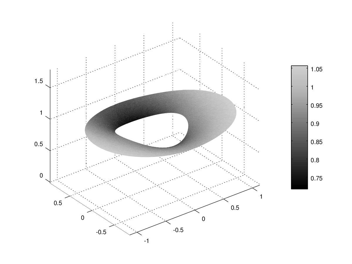
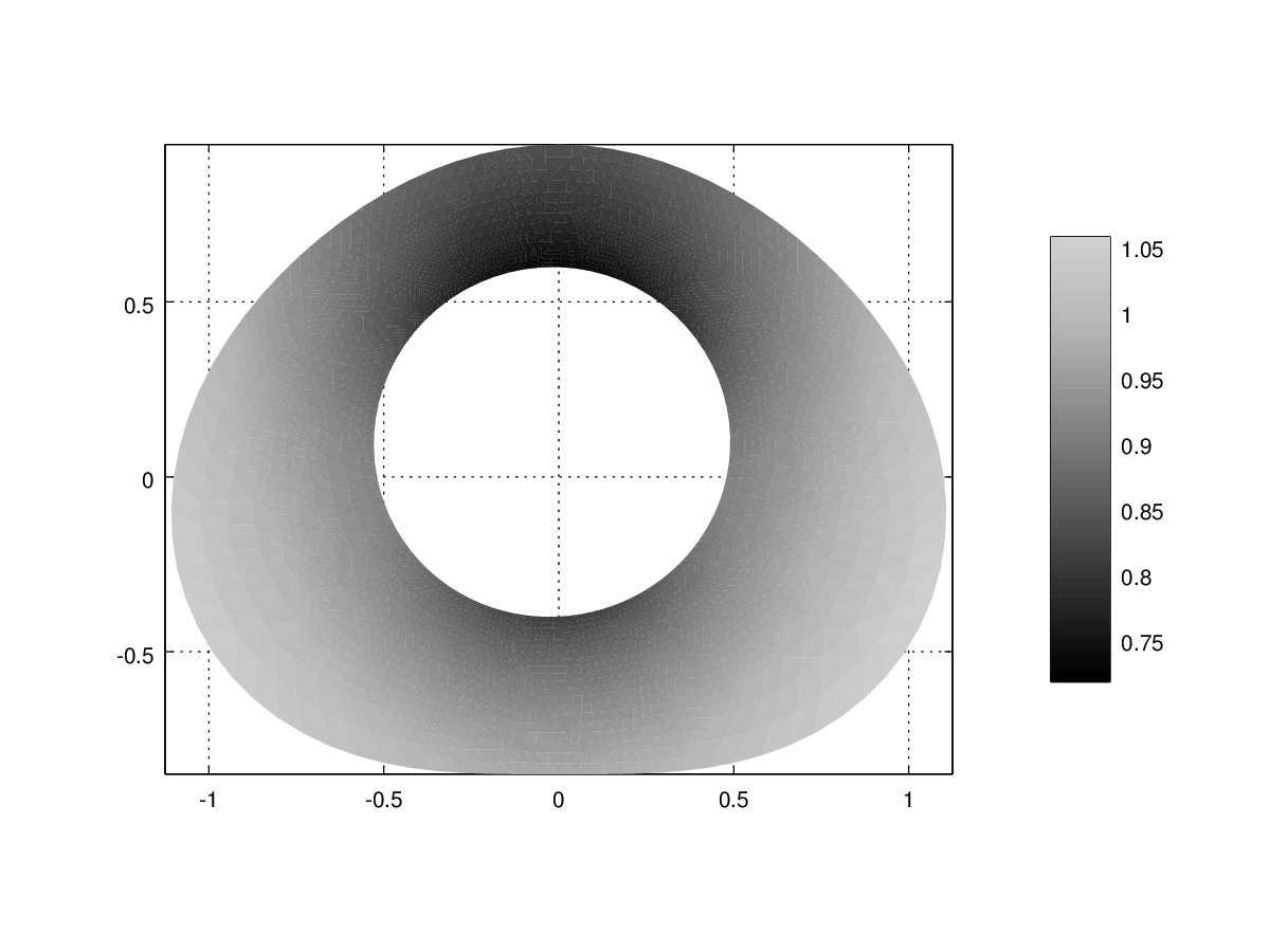
Figure 1. Exact solution.

Then we corrupt the Dirichlet data $g_{D}$ pointwise with a normal noise having zero mean and variance one, to obtained the corrupted Dirichlet data $g_{D}^{\delta}$. The noise is scaled so that

$$\|g_{D}^{\delta}-g_{D}\|_{\infty}=\alpha\|g_{D}\|_{\infty}$$

that is the relative amplitude of noise in $L^{\infty}$-norm is $\alpha$. In the experiments, we have chosen $\alpha=1\%$, $2\%$ and $5\%$. The exact Neumann data is used (i.e. $g_{N}^{\delta}=g_{N}$), as in practical situations it is the imposed data (the net current), whereas the $g_{D}$ is the measured data (the corresponding voltages). Therefore $g_{N}$ is known quite precisely compared to $g_{D}$. We then compute the corresponding amplitude of noise for the $L^{2}$ norm $\delta=\delta(\alpha,\|g_{D}\|_{\infty})$, which defined our stopping criterion for the iteration of the method.

The iterated quasi-reversibility problem is then solved using a conforming finite-element method using $P_{2}$ Lagrange finite elements for $u_{\varepsilon}^{M}$ and $RT_{1}$ Raviart-Thomas finite elements for $\mathbf{p}_{\varepsilon}^{M}$ [39]. The study of convergence of the finite-element approximation of the quasi-reversibility approximation toward the continuous solution is just a slight adaptation of section 4.4 in [31], as the formulations are quite similar, and therefore is omitted in the present study. To avoid an inverse crime, the direct and inverse problems are solved on different meshes.

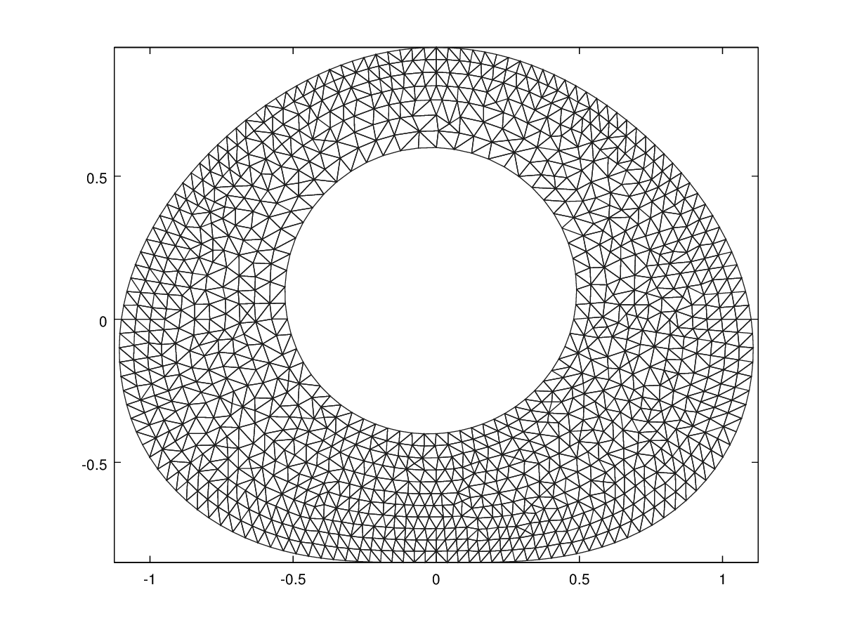
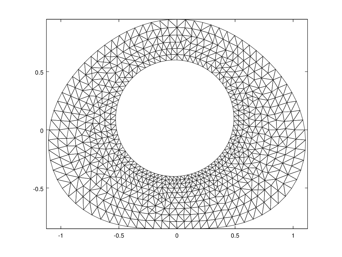
Figure 2. The direct and inverse meshes used in the numerical simulation.

According to our study, the choice of $\varepsilon$ is completely arbitrary in the iterated quasi-reversibility method. Therefore, we have chosen $\varepsilon=1$ in the experiments, as it leads to a good conditioning of the finite-element matrices.

First of all, we present in figure 3 the evolution of the residual

$$\sqrt{\|\nabla\cdot\mathbf{p}_{\varepsilon}^{M}\|_{L^{2}(\Omega)}^{2}+\|\nabla u_{\varepsilon}^{M}-\mathbf{p}_{\varepsilon}^{M}\|_{L^{2}(\Omega)}^{2}+\|u_{\varepsilon}-g_{D}^{\delta}\|_{L^{2}(\Gamma)}^{2}+\|\mathbf{p}_{\varepsilon}\cdot\nu-g_{N}^{\delta}\|_{L^{2}(\Gamma)}}$$

until the stopping criterion is reached. As expected theoretically, the greater is the noise, the smaller is $M(\delta)$.

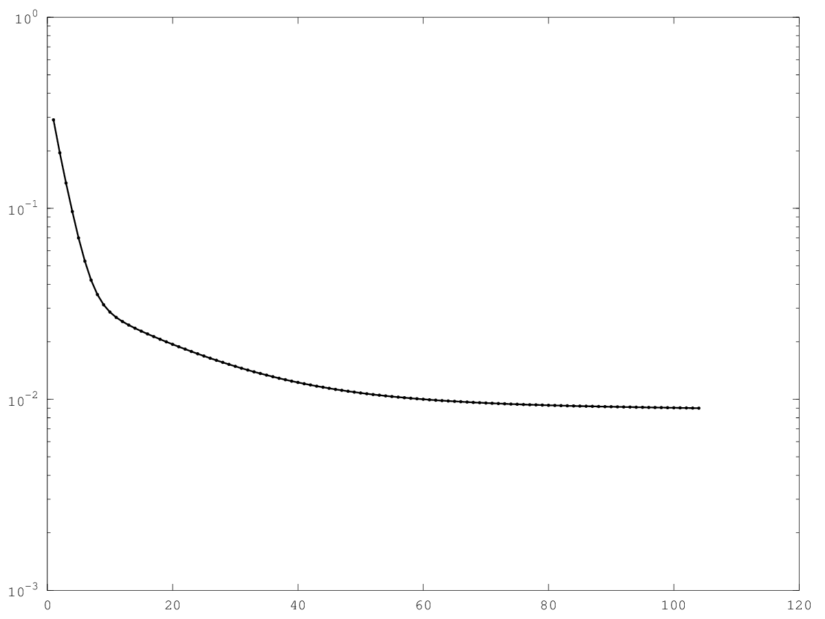
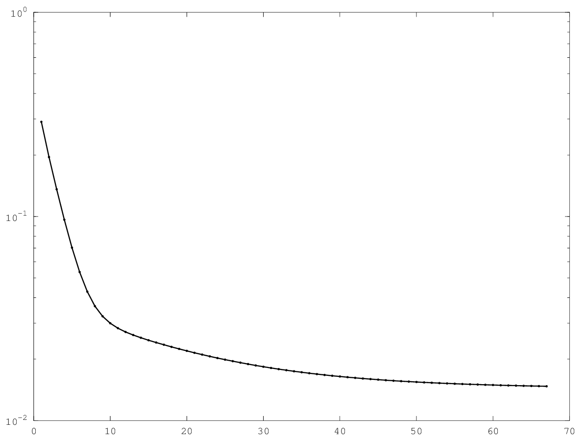
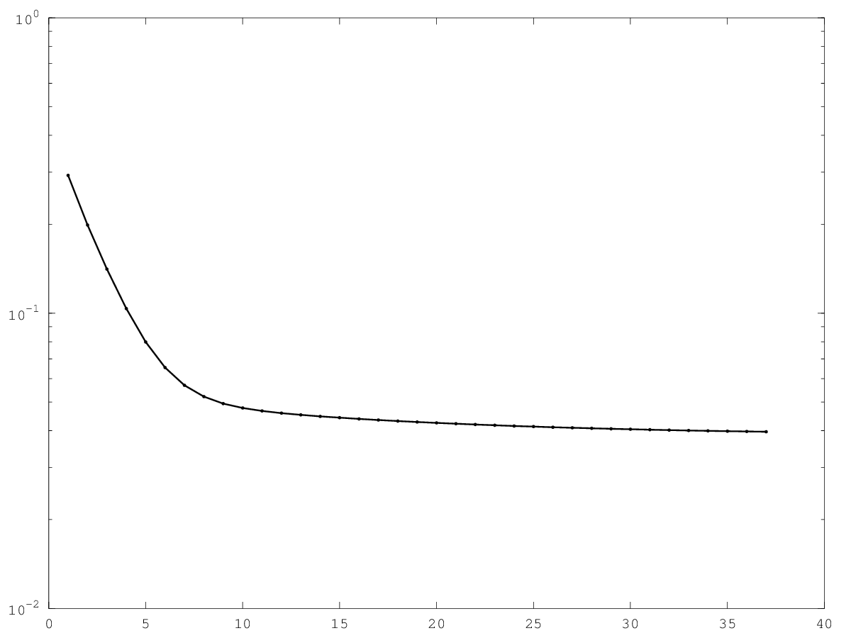
Figure 3. Residual vs. number of iterations, until stopping criterion is reached, for $\alpha$ = $1\%$, $2\%$ and $5\%$.

Now we present the reconstruction results: in figure 4, the exact solution is compared to the reconstructed one in the whole domain of study. In figure 5, we focus on the boundary $\Gamma$: we compare the exact data $g_{D}$, the noisy one $g_{D}^{\delta}$ used in the iterated quasi-reversibility method, and finally the trace of the reconstructed solution $u_{\varepsilon}^{M(\delta)}$. Note that the iterated quasi-reversibility method gives good result even with severely corrupted data.

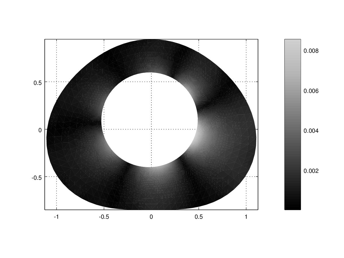
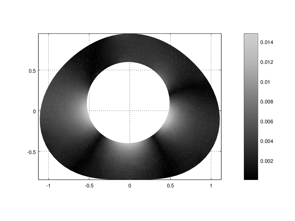
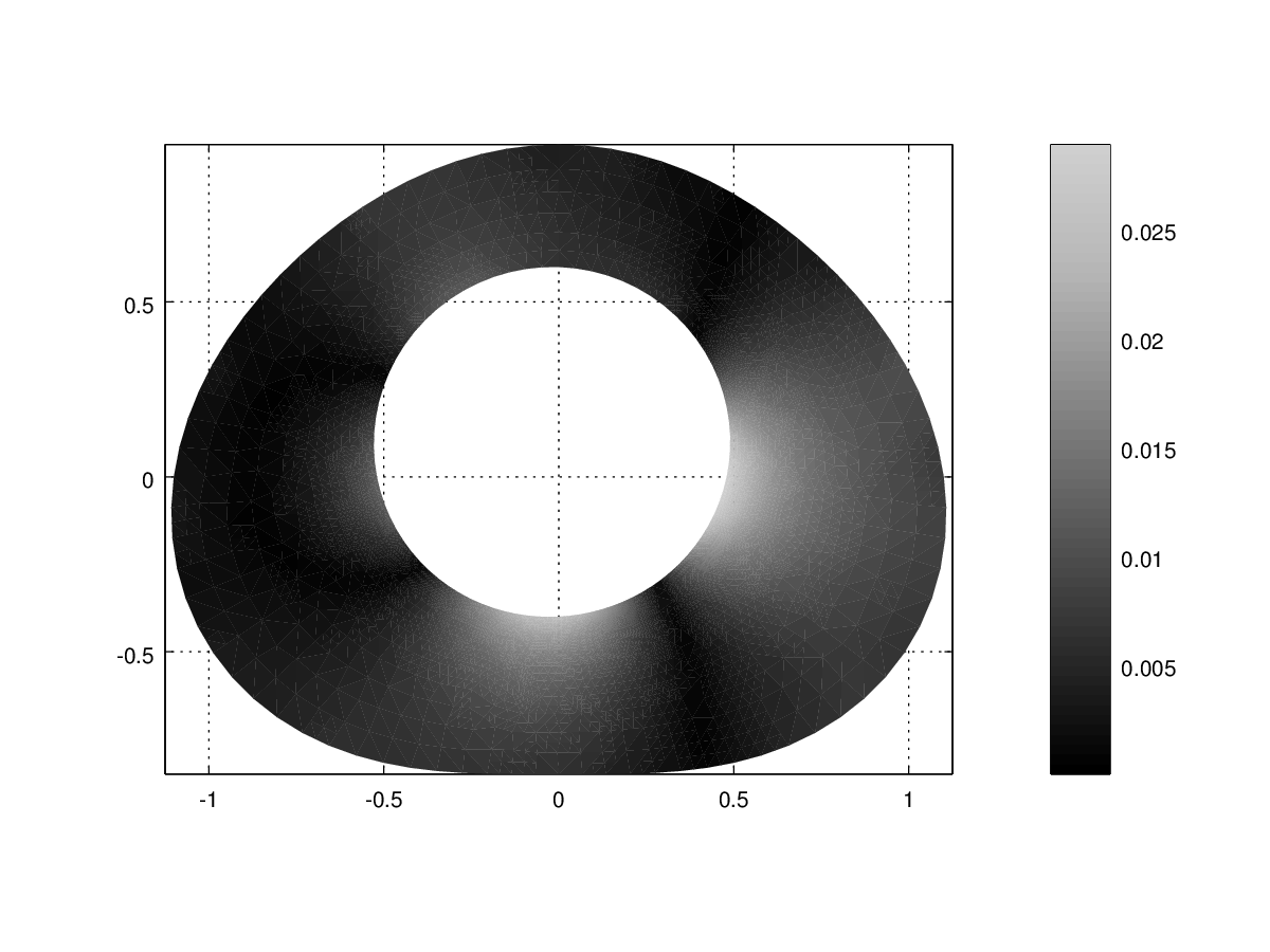
Figure 4. $|u_{\varepsilon}^{M(\delta)}-u|$, for $\alpha$ = $1\%$, $2\%$ and $5\%$.

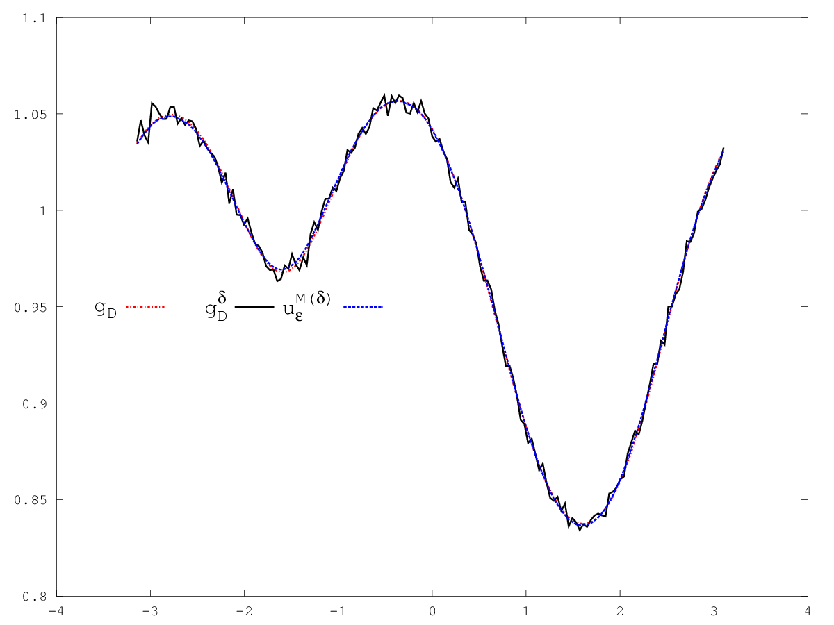
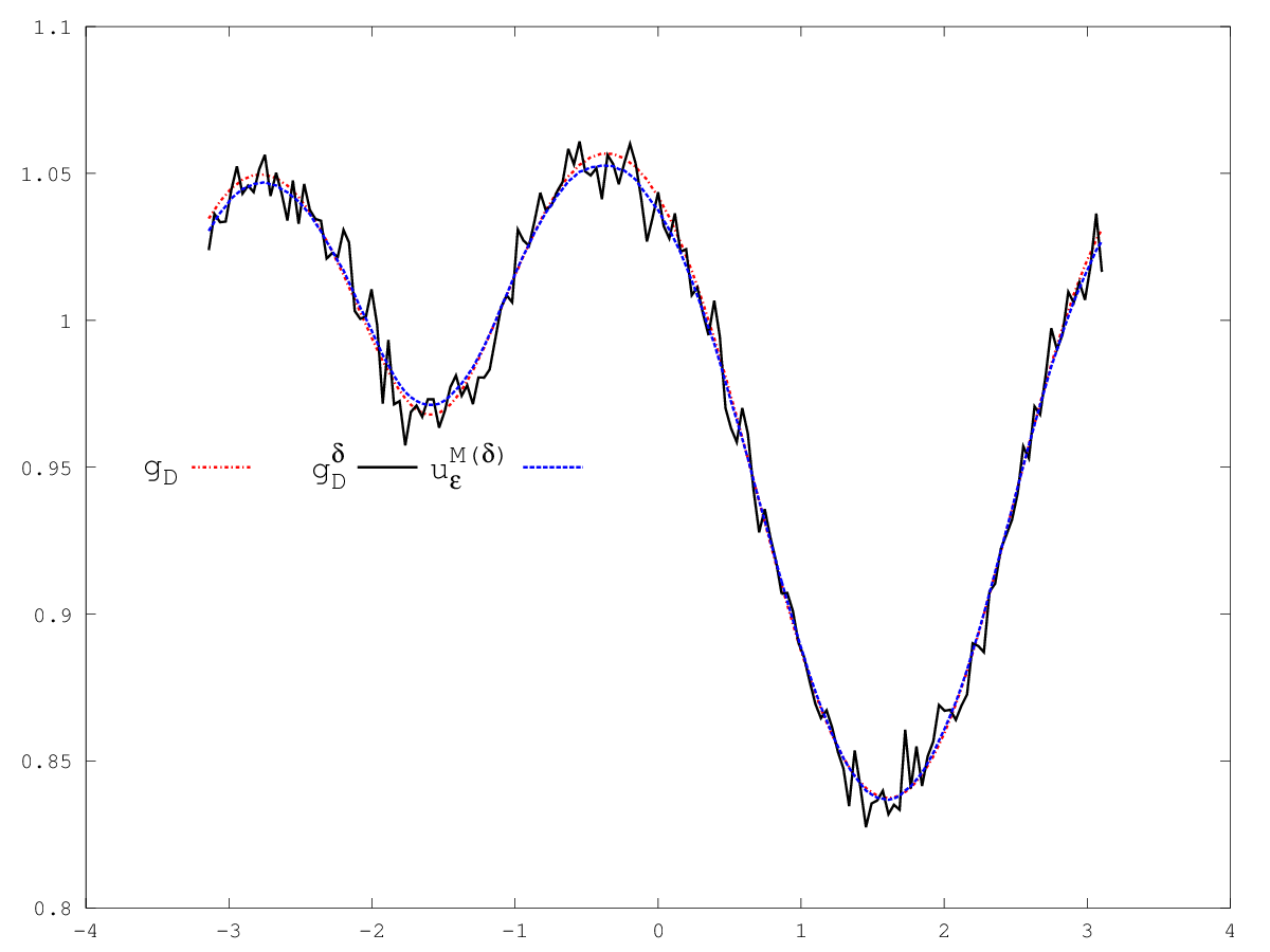
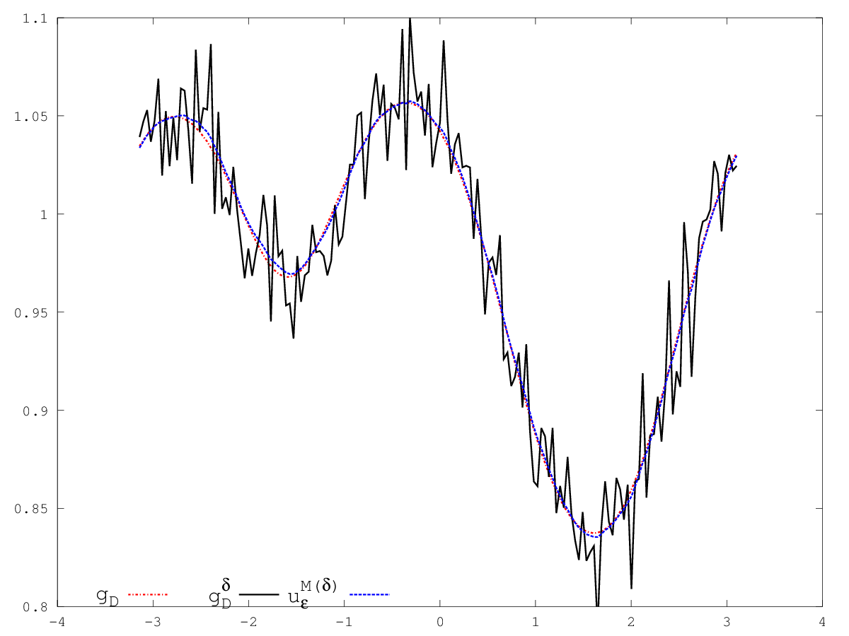
Figure 5. Exact Dirichlet data, noisy Dirichlet data, and trace of $u_{\varepsilon}^{M(\delta)}$ on $\Gamma$, for $\alpha$ = $1\%$, $2\%$ and $5\%$.

Finally, on figure 6, we present the reconstructed Robin coefficient on $\Gamma_{c}$, which was our main objective. Again, the reconstruction is still acceptable for high level of noise on the data.

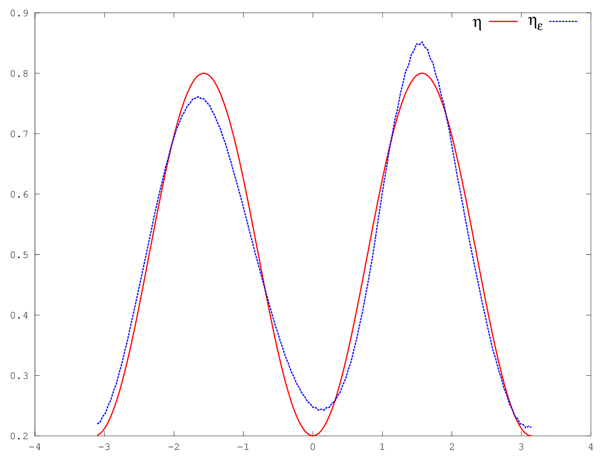
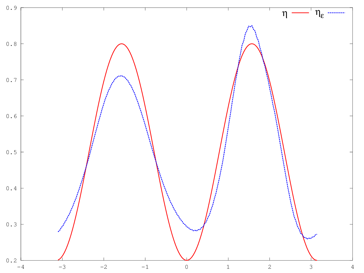
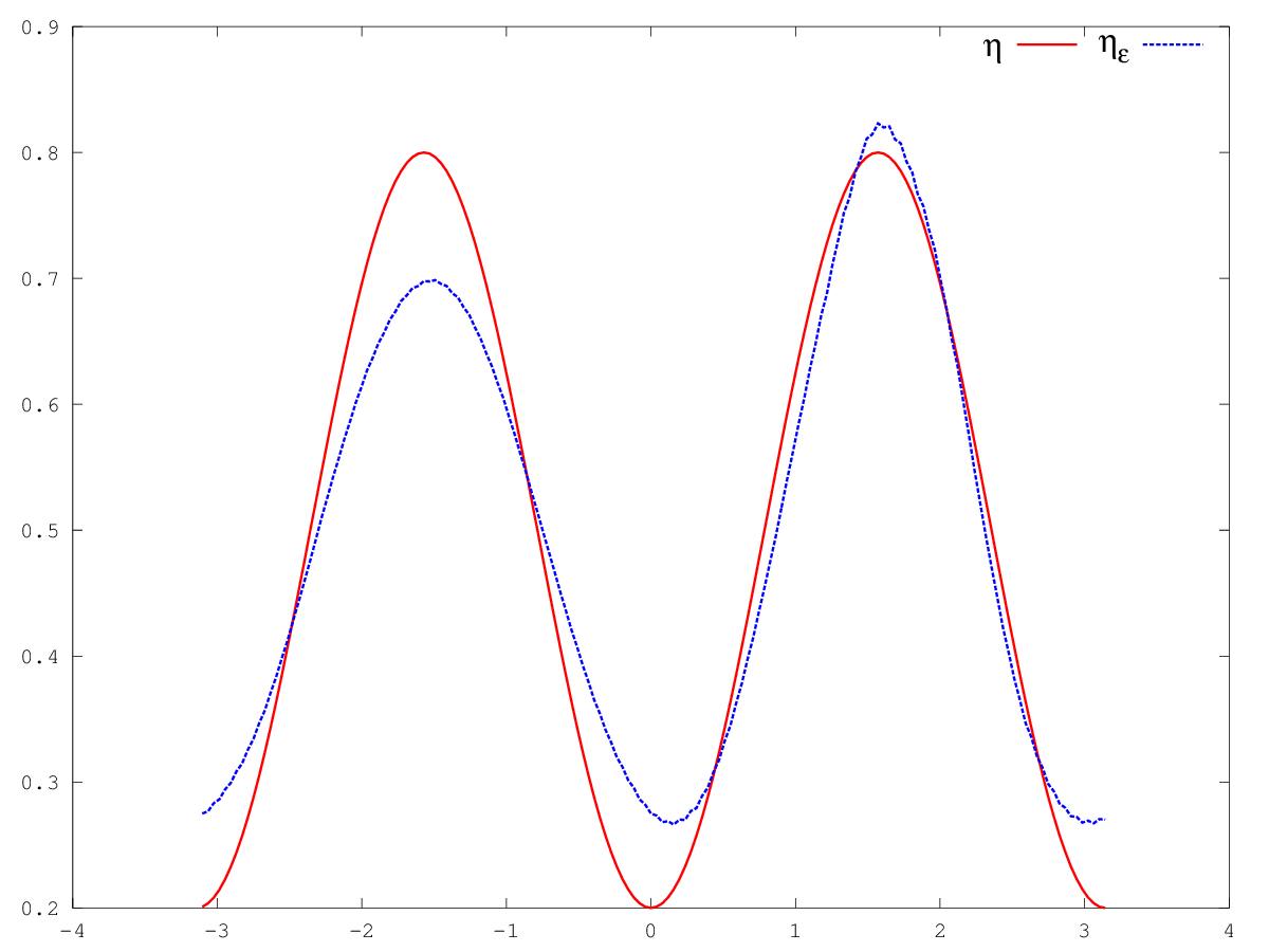
Figure 6. Exact ($\eta$) and reconstructed ($\eta_{\varepsilon}$) Robin coefficient on $\Gamma_{c}$, for $\alpha$ = $1\%$, $2\%$ and $5\%$.

6.2. One-dimensional heat equation

We now focus on the data-completion problem for a one-dimensional heat equation. The problem reads: find $u\in H^{1,1}((0,T)\times(a,b))$ such that

$$\left\{\begin{array}[]{cccl}\partial_{t}u&=&\partial_{xx}u&\text{in }(0,T)\times(a,b)\\ u(t,a)&=&g_{D}^{\delta},&\ t\in(0,T)\\ \partial_{x}u(t,a)&=&g_{N}^{\delta},&\ t\in(0,T).\end{array}\right.$$

Note that, as $\partial_{xx}u=\partial_{t}u\in L^{2}(0,T;L^{2}(a,b))$, we have $p:=\partial_{x}u\in L^{2}(0,T;H^{1}(a,b))$, and hence $g_{N}(t)=p(a,t)\in L^{2}(0,T)$ without additional assumption, which is not the case for the multi-dimensional case. Hence the equivalent data-completion problem with additional unknown $p$ reads: for $(g_{D}^{\delta},g_{N}^{\delta})\in L^{2}(0,T)\times L^{2}(0,T)$, find $u\in H^{1,1}((0,T)\times(a,b))$ and $p\in L^{2}(0,T;H^{1}(a;b))$ such that

$$\left\{\begin{array}[]{cccl}\partial_{t}u&=&\partial_{x}p&\text{in }(0,T)\times(a,b)\\ \partial_{x}u&=&p&\text{in }(0,T)\times(a,b)\\ u(t,a)&=&g_{D}^{\delta},&\ t\in(0,T)\\ p(t,a)&=&g_{N}^{\delta},&\ t\in(0,T).\end{array}\right.$$

According to our study, the quasi-reversibility regularization of this problem is: for $\varepsilon>0$, find $u_{\varepsilon}\in H^{1,1}((0,T)\times(a,b))$ and $p_{\varepsilon}\in L^{2}(0,T;H^{1}(a,b))$ such that for all $v\in H^{1,1}((0,T)\times(a,b))$, for all $q\in L^{2}(0,T;H^{1}(a,b))$

$$\int_{0}^{T}\int_{a}^{b}\Big{(}(\partial_{t}u_{\varepsilon}-\partial_{x}p_{\varepsilon})\,(\partial_{t}v-\partial_{x}q)+(\partial_{x}u_{\varepsilon}-p_{\varepsilon})\,(\partial_{x}v-q)\Big{)}\,dx\,dt$$

$$+\int_{0}^{T}\Big{(}u_{\varepsilon}(s,a)\,v(s,a)+p_{\varepsilon}(a,s)\,q(a,s)\Big{)}\,dt+\varepsilon\int_{0}^{T}\int_{a}^{b}\Big{(}\partial_{t}u_{\varepsilon}\,\partial_{t}v+\partial_{x}u_{\varepsilon}\,\partial_{x}v+p_{\varepsilon}\,q\Big{)}\,dx\,dt$$

$$=\int_{0}^{T}\Big{(}g_{D}^{\delta}(s)\,v(s,a)+g_{N}^{\delta}(s)\,q(s,a)\Big{)}\,ds,$$

and the iterated quasi-reversibility method: for $\varepsilon>0$, define $(u_{\varepsilon}^{-1},p_{\varepsilon}^{-1})=(0,0)$ and for all $M\in\mathbb{N}$, $u_{\varepsilon}^{M}\in H^{1,1}((0,T)\times(a,b))$ and $p_{\varepsilon}^{M}\in L^{2}(0,T;H^{1}(a,b))$ are such that for all $v\in H^{1,1}((0,T)\times(a,b))$, for all $q\in L^{2}(0,T;H^{1}(a,b))$,

$$\int_{0}^{T}\int_{a}^{b}\Big{(}(\partial_{t}u_{\varepsilon}^{M}-\partial_{x}p_{\varepsilon}^{M})\,(\partial_{t}v-\partial_{x}q)+(\partial_{x}u_{\varepsilon}^{M}-p_{\varepsilon}^{M})\,(\partial_{x}v-q)\Big{)}\,dx\,dt$$

$$+\int_{0}^{T}\Big{(}u_{\varepsilon}^{M}(s,a)\,v(s,a)+p_{\varepsilon}^{M}(a,s)\,q(a,s)\Big{)}\,dt+\varepsilon\int_{0}^{T}\int_{a}^{b}\Big{(}\partial_{t}u_{\varepsilon}^{M}\,\partial_{t}v+\partial_{x}u_{\varepsilon}^{M}\,\partial_{x}v+p_{\varepsilon}^{M}\,q\Big{)}\,dx\,dt$$

$$=\int_{0}^{T}\Big{(}g_{D}^{\delta}(s)\,v(s,a)+g_{N}^{\delta}(s)\,q(s,a)\Big{)}\,ds+\varepsilon\int_{0}^{T}\int_{a}^{b}\Big{(}\partial_{t}u_{\varepsilon}^{M-1}\,\partial_{t}v+\partial_{x}u_{\varepsilon}^{M-1}\,\partial_{x}v+p_{\varepsilon}^{M-1}\,q\Big{)}\,dx\,dt.$$

We discretize the space $H^{1,1}(\mathcal{Q})$ and $L^{2}(0,T;H^{1}(a,b))$ using a tensorial product of Lagrange finite elements, namely $P^{1}\otimes P^{1}$ finite elements for $H^{1,1}$ and $P^{0}\times P^{1}$ for $L^{2}(H^{1})$.

In our simulations, we choose $T=1$, $a=1$ and $b=2$. We consider two exact solution of the heat equation $\displaystyle u_{1}(t,x):=\frac{1}{8}\left(\frac{x^{3}}{3}+x\,(1+2\,t)\right)$ and $\displaystyle u_{2}(t,x):=e^{-t/4}\sin\left(t/2\right)$.

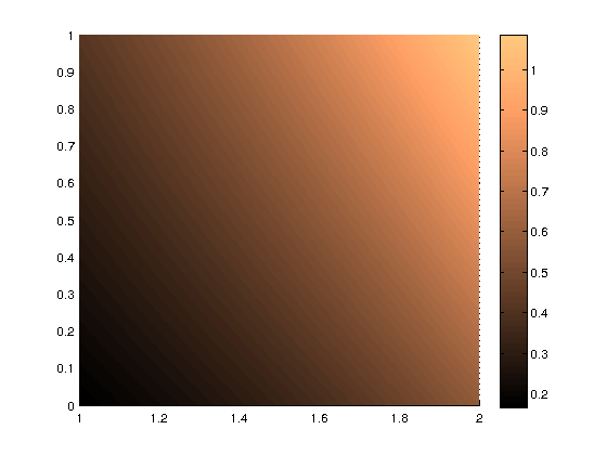
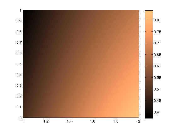
Figure 7. Exact solutions $u_{1}$ and $u_{2}$ in $\mathcal{Q}$.

The corresponding exact data $(g_{D},g_{N})$ are corrupted pointwise by a normal noise with zero means and variance one, which is scaled so that the noisy data $(g_{D}^{\delta},g_{N}^{\delta})$ verifies

$$\|g_{D}^{\delta}-g_{D}\|_{\infty}=\alpha\|g_{D}\|_{\infty},\quad\|g_{N}^{\delta}-g_{N}\|_{\infty}=\alpha\|g_{N}\|_{\infty}.$$

In our experiments, we test our method with $\alpha=2\%$ and $\alpha=5\%$. As in the elliptic case, we choose $\varepsilon=1$, and stop the iterations of the method once the stopping criterion is reached.

In figures 8 and 9, we present the relative error over $\mathcal{Q}$, defined as the ratio

$$\frac{u_{\varepsilon}^{M}(\delta)-u}{\|u\|_{\infty}}$$

for both solutions $u_{1}$ and $u_{2}$. We see that the iterated quasi-reversibility method gives also good reconstruction for this parabolic problem, even for high level of noise on both Dirichlet and Neumann data.

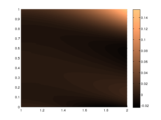
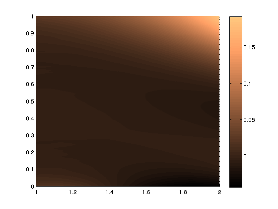
Figure 8. Relative error $(u_{1\varepsilon}^{M(\delta)}-u_{1})/\|u_{1}\|_{\infty}$ in $\mathcal{Q}$. Left: $\alpha=2\%$. Right: $\alpha=5\%$.

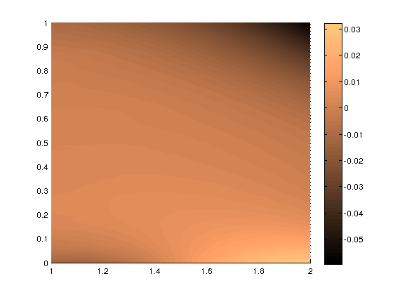
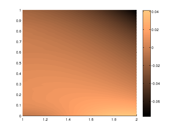
Figure 9. Relative error $(u_{2\varepsilon}^{M(\delta)}-u_{2})/\|u_{2}\|_{\infty}$ in $\mathcal{Q}$. Left: $\alpha=2\%$. Right: $\alpha=5\%$.

Finally, in figures 10, we present the evolution of the residual quantity

$$\sqrt{\|\partial_{t}u_{\varepsilon}^{M}-\partial_{x}p_{\varepsilon}^{M}\|_{L^{2}(\mathcal{Q})}^{2}+\|\partial_{x}u_{\varepsilon}^{M}-p_{\varepsilon}^{M}\|_{L^{2}(\mathcal{Q})}^{2}+\|u_{\varepsilon}^{M}(.,a)-g_{D}^{\delta}\|_{L^{2}(0,T)}^{2}+\|p_{\varepsilon}^{M}(.,a)-g_{N}^{\delta}\|_{L^{2}(0,T)}^{2}}$$

during the iterations of the method, until the stopping criterion is reached.

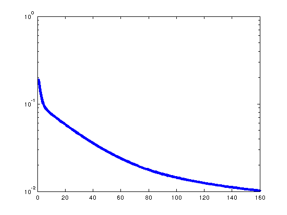
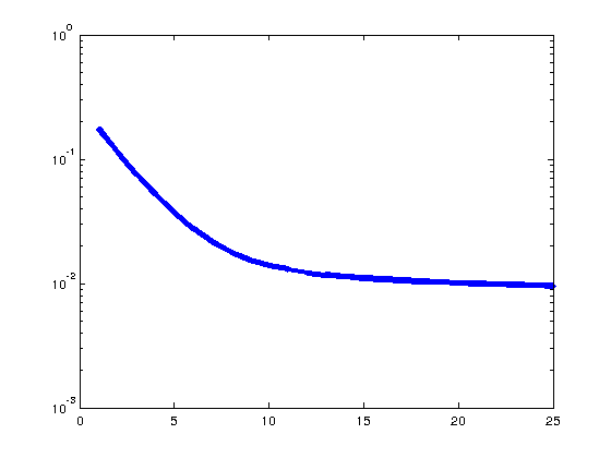
Figure 10. Residual vs. number of iterations, until stopping criterion is reached, for $\alpha=5\%$. Exact solution: left $u_{1}$, right $u_{2}$.

References

- [1] (MR2565570 ) [10.1088/0266-5611/25/12/123004] G. Alessandrini, L. Rondi, E. Rosset and S. Vessella, The stability for the Cauchy problem for elliptic equations, Inverse problems, 25 (2009), 123004.
- [2] [10.1088/0266-5611/23/2/020] F. Ben Belgacem, Why is the Cauchy problem severely ill-posed?, Inverse problems, 23 (2007), 823-836.
- [3] [10.1137/1.9781611972030] P. Grisvard, Elliptic Problems in Nonsmooth Domains, Classic in Applied Mathematics, SIAM, 2011.
- [4] [10.1051/cocv/2011168] J. Le Rousseau and G. Lebeau, On Carleman estimates for elliptic and parabolic operators. Applications to unique continuation and control of parabolic equations, ESAIM Control Optim. Calc. Var., 18 (2012), 712-747.
- [5] A. Ben Abda, J. Blum, C. Boulbe and B. Faugeras, Minimization of an energy error functional to solve a Cauchy problem arising in plasma physics: the reconstruction of the magnetic flux in the vacuum surrounding the plasma in a Tokamak, ARIMA 15 (2012).
- [6] [10.1016/j.jcp.2011.04.005] J. Blum, C. Boulbe and B. Faugeras Reconstruction of the equilibrium of the plasma in a Tokamak and identification of the current density profile in real time, Journal of Computational Physics, 231 (2012), 960–980.
- [7] L. Baratchart, L. Bourgeois, J. Leblond, Uniqueness results for inverse Robin problems with bounded coefficient, preprint, \arXiv1412.3283.
- [8] [10.1088/0266-5611/19/4/312] G. Alessandrini, L. Del Piero and L Rondi, Stable determination of corrosion by a single electrostatic boundary measurement , Inverse problems, 19 (2003), 973.
- [9] [10.1088/0266-5611/23/3/027] E. Sincich, Lipschitz stability for the inverse Robin problem, Inverse problems, 23 (2007), 1311.
- [10] [10.1088/0266-5611/15/6/303] S. Chaabane and M. Jaoua, Identification of Robin coefficients by the means of boundary measurements, Inverse problems, 15 (1999), 1425.
- [11] [10.1088/0266-5611/15/1/008] D. Fasino and G. Inglese, An inverse Robin problem for Laplace’s equation: theoretical results and numerical methods, Inverse problems, 15 (1999), 41.
- [12] [10.1088/0266-5611/22/1/007] S. Andrieux, T.N. Baranger and A. Ben Abda, Solving Cauchy problems by minimizing an energy-like functional, Inverse problems, 22 (2006), 115.
- [13] [10.1088/0266-5611/17/3/313] A. Cimetière, F. Delvare, M. Jaoua and F. Pons, Solution of the Cauchy problem using iterated Tikhonov regularization, Inverse problems, 17 (2001), 553.
- [14] [10.1088/0266-5611/27/4/045005] F. Ben Belgacem, D. T. Du and F. Jelassi, Extended-domain-Lavrentiev’s regularization for the Cauchy problem, Inverse Problems, 27 (2011), 045005.
- [15] [10.1088/0266-5611/22/4/012] M. Azaïez, F. Ben Belgacem and H. El Fekih, On Cauchy’s problem: II. Completion, regularization and approximation, Inverse Problems, 22 (2006), 1307.
- [16] [10.1088/0266-5611/31/3/035011] Y. Boukari and H. Haddar, A Convergent Data Completion Algorithm Using Surface Integral Equations, Inverse Problems, 31 (2015), 035011.
- [17] E. Burman, A stabilized nonconforming finite element method for the elliptic Cauchy problem, preprint, \arXiv1406.4385.
- [18] R. E. Puzyrev and A. A. Shlapunov, On an Ill-Posed Problem for the Heat Equation, Journal of Siberian Federal University, 5 (2012), 337-348.
- [19] R. Lattès and J. L. Lions, The Method of Quasi-reversibility: Applications to Partial Differential Equations, American Elsevier Publishing Company, 1969.
- [20] [10.1137/0151085] M. V. Klibanov and F. Santosa, A Computational Quasi-Reversibility Method for Cauchy Problems for Laplace’s Equation, SIAM Journal on Applied Mathematics, 51 (1991), 1653–1675.
- [21] [10.1137/06066970X] C. Clason and M. V. Klibanov, The Quasi-Reversibility Method for Thermoacoustic Tomography in a Heterogeneous Medium, SIAM Journal on Scientific Computing, 30 (2007), 1–23.
- [22] [10.1088/0266-5611/21/3/018] L. Bourgeois, A mixed formulation of quasi-reversibility to solve the Cauchy problem for Laplace’s equation, Inverse Problems, 21 (2005), 1087.
- [23] [10.1088/0266-5611/22/2/002] L. Bourgeois, Convergence rates for the quasi-reversibility method to solve the Cauchy problem for Laplace’s equation, Inverse Problems, 22 (2006), 413.
- [24] [10.1088/0266-5611/25/3/035005] H. Cao, M. V. Klibanov and S. V. Pereverzev, A Carleman estimate and the balancing principle in the quasi-reversibility method for solving the Cauchy problem for the Laplace equation, Inverse Problems, 25 (2009), 035005.
- [25] [10.1088/0266-5611/26/9/095016] L. Bourgeois and J. Dardé, A duality-based method of quasi-reversibility to solve the Cauchy problem in the presence of noisy data, Inverse Problems, 26 (2010), 095016.
- [26] [10.3934/ipi.2010.4.351] L. Bourgeois and J. Dardé, A quasi-reversibility approach to solve the inverse obstacle problem, Inverse Problems and Imaging, 4 (2010), 351-377.
- [27] [10.1088/0266-5611/28/1/015008] J. Dardé, The ’exterior approach’: a new framework to solve inverse obstacle problems, Inverse Problems, 28 (2012), 015008.
- [28] [10.3934/ipi.2014.8.23] L. Bourgeois and J. Dardé, The ”exterior approach” to solve the inverse obstacle problem for the Stokes system, Inverse Problems and Imaging, 8 (2014), 23-51.
- [29] [10.1155/S1025583499000041] K. A. Ames and L. E. Payne, Continuous dependence on modeling for some well-posed perturbations of the backward heat equation, Journal of Inequalities and Applications, (1999).
- [30] G. W. Clark and S. F. Oppenheimer, Quasireversibility methods for non-well-posed problems, Electronic Journal of Differential Equations, 8 1994, 1-9.
- [31] [10.1137/120895123] J. Dardé, A. Hannukainen and N. Hyvönen An -Based Mixed Quasi-reversibility Method for Solving Elliptic Cauchy Problems, SIAM J. Numer. Anal., 51 2013, 2123–2148.
- [32] [10.1142/S0218202597000487 ] P. Fernandes and G. Gilardi Magnetostatic and Electrostatic Problems in Inhomogeneous Anisotropic Media with Irregular Boundary and Mixed Boundary Conditions, Math. Models Methods Appl. Sci., 7 (1997).
- [33] [10.1137/S0036139994277828] K. Bryan and L. F. Caudill, Jr., An inverse problem in thermal imaging, SIAM J. Appl. Math., 56 (1996), pp. 715 – 735.
- [34] [10.1137/110855703] H. Harbrecht and J. Tausch, On the numerical solution of a shape optimization problem for the heat equation, SIAM J. Sci. Comput., 35 (2013), pp. A104 –- A121.
- [35] [10.1088/0266-5611/25/7/075005] M. Ikehata and M. Kawashita, The enclosure method for the heat equation, Inverse Problems, 25 (2009), pp. 075005, 10.
- [36] H. W. Engl, M. Hanke and A. Neubauer, Regularization of inverse problems, Mathematics and its Applications, 375. Kluwer Academic Publishers Group, Dordrecht, 1996.
- [37] A.N. Tykhonov, Solution of incorrectly formulated problems and the regularization method, Soviet Math. Dokl., 4 (1063).
- [38] [10.1007/978-0-387-70914-7] H. Brezis, Functional analysis, Sobolev spaces and partial differential equations, Universitext. Springer, New York, 2011.
- [39] [10.1137/1.9780898719208] P.G. Ciarlet, The Finite Element Method for Elliptic Problems, Classics in Applied Mathematics, SIAM, 2002.