Semi-Lagrangian discontinuous Galerkin schemes for some first- and second-order partial differential equations

Abstract.

Explicit, unconditionally stable, high-order schemes for the approximation of some first- and second-order linear, time-dependent partial differential equations (PDEs) are proposed. The schemes are based on a weak formulation of a semi-Lagrangian scheme using discontinuous Galerkin (DG) elements. It follows the ideas of the recent works of Crouseilles, Mehrenberger and Vecil (2010), Rossmanith and Seal (2011), for first-order equations, based on exact integration, quadrature rules, and splitting techniques for the treatment of two-dimensional PDEs. For second-order PDEs the idea of the scheme is a blending between weak Taylor approximations and projection on a DG basis. New and sharp error estimates are obtained for the fully discrete schemes and for variable coefficients. In particular we obtain high-order schemes, unconditionally stable and convergent, in the case of linear first-order PDEs, or linear second-order PDEs with constant coefficients. In the case of non-constant coefficients, we construct, in some particular cases, ”almost” unconditionally stable second-order schemes and give precise convergence results. The schemes are tested on several academic examples.

1. Introduction

In this paper we consider equations of the form

$$u_{t}-\frac{1}{2}Tr(\sigma\sigma^{T}D^{2}u)+b\cdot\nabla u+ru=0,\quad x\in\Omega,\ t\in(0,T),$$ (1)

where $\Omega\subset\mathbb{R}^{d}$ is a box (with some boundary conditions on $\partial\Omega$), $\sigma$ (matrix), $b$ (vector) and $r$ (scalar) may be $x$-dependent, at least Lipschitz continuous, together with an initial condition

$$u(0,x)=u_{0}(x),\quad x\in\Omega,$$ (2)

with $u_{0}\in L^{2}(\Omega)$. The matrix $\sigma$ may be zero or positive semidefinite. Unless otherwise stated, we will in general assume periodic boundary conditions for (1) in order to avoid difficulties on the boundary. We will assume sufficient regularity on the data in order to have existence and uniqueness of weak solutions of (1)-(2), and so that $t\rightarrow u(t,.)$ is in $C^{0}([0,T],L^{2}(\Omega))$.

We study and propose new semi-Lagrangian Discontinuous Galerkin schemes, also abbreviated ”SLDG” in this work, in order to approximate the solutions of (1)-(2).

The semi-Lagrangian (SL) approach (see [13], or the textbook [14]), is based on the approximation of the ”method of characteristics”. By considering a weak formulation of this principle, an explicit SLDG scheme is obtained. In the case of first-order PDEs with constant coefficient, our approach is based on a similar method as in the recent works of Crouseilles, Mehrenberger and Vecil [9] (for the Vlasov equation in plasma physics), Rossmanith and Seal [34]. However our approach seems not to have been considered for variable coefficients. It is slightly different from the work of Qiu and Shu [31] (see also Restelli et al [32]), where first a weak formulation of the PDE is considered, and then quadrature formulae are used (see also [33] for the original approach). Here we will furthermore introduce new SLDG schemes for second-order PDEs for which we prove stability and convergence results, and obtain higher-orders of accuracy when possible.

First, in Section 2, we revisit the one-dimensional first-order advection equation with non-constant advection term $b(x)$ (case $\sigma=0$ in (1)). We give a new unconditional stability result, and convergence proof, extending similar results of [9], [34] (or [31]) that was obtained for the case of a constant advection term. The unconditional stability property can be interesting when compared to a standard DG approach where a restrictive CFL condition must in general be considered [7].

Based on the operator construction for first-order advection, we then introduce, in Section 3, new schemes for linear second-order PDEs of type (1), in the form of explicit high-order SLDG schemes. These schemes are based, for the temporal discretization, on the use of ”weak Taylor approximations”, see in particular the review book by Kloeden and Platen [20] (see also Kushner [21] and the review book by Kushner and Dupuis [22], Platen [30], Milstein [25], Talay [37], Pardoux and Talay [28], Menaldi [24], Camilli and Falcone [4], Milstein and Tretyakov [26], [10]). Such approximations where used by R. Ferretti in [16] as well as in Debrabant and Jakobsen [11] in the context of semi-Lagrangian schemes, using interpolation methods for the space variable. The problem of coupling such approximations with a spatial grid approximation, in particular using a high-order interpolation method, can be the stability and the convergence proof of the method. The $P_{1}$ interpolation is known to be $L^{\infty}$ stable, but it is only second-order accurate in space (for regular data). Some higher-order SL approximations have been proved to be stable (and convergent) for specific equations and under large CFL numbers (see [15, 5]), or for some advection equations when the SL scheme can be reinterpreted in a weak form (we refer in particular to Ferretti’s work [16, 17]).

The schemes of the present paper can be seen as projections of these approximation on a discontinous Galerkin basis. We will in particular propose a second-order approximation (in time) corresponding to a Platen’s scheme [20, Chapter 14], but higher-order approximations (in time) could be obtained in the same way. The scheme will be proved to be also high-order in space, stable and convergent under a weak CFL condition (of the form ${\Delta x}^{4}\leq\lambda{\Delta t}$ for some constant $\lambda$, where ${\Delta t}$ and ${\Delta x}$ denote the time and mesh steps).

For the more simple case of second-order PDEs with constant coefficients, we also propose explicit and unconditionally stable schemes, high-order in space and up to third-order in time (higher-order can be obtained [2]).

In section 4 we consider extensions to some linear two-dimensional PDEs. For first-order PDEs, we show how to combine the scheme with higher-order splitting techniques, like Strang’s splitting, but also Ruth’s third-order splitting [35], Forest’s fourth-order splitting [18] and Yoshida’s sixth-order splitting [40] (see also [19] and [41]). A splitting strategy to treat general second-order PDEs with constant coefficients is explained. The case of second-order PDEs with variable diffusion coefficients is discussed but only treated in some specific cases (see Remark 4.4 as well as Example 7 and Example 8 of Section 5). The general case will be treated in a forthcoming work (see however Remark 4.3).

Finally in Section 5 we show the relevance of our approach on several academic numerical examples in one and two dimensions (using Cartesian meshes), including also a Black and Scholes PDE in mathematical finance.

The advantage of the proposed schemes is that they combine the DG framework which allows high-order spatial accuracy and the potential of degree adaptivity, together with unconditional stability properties in the $L^{2}$ norm from the weak formulation of the semi-Lagrangian scheme.

Note that our general strategy is to use a Cartesian grid, a particular one-dimensional advection scheme, and splitting techniques (for more standard Discontinuous Galerkin approaches, see for instance [8] or [29]).

Ongoing works using the current approach concern the construction of higher-order schemes for general second-order PDEs [2], extensions to nonlinear PDEs arising from deterministic control [3] or from stochastic control.

Acknowledgments. This work was partially supported by the EU under the 7th Framework Programme Marie Curie Initial Training Network “FP7-PEOPLE-2010-ITN”, SADCO project, GA number 264735-SADCO. The first author also wishes to thank K. Debrabant for pointing out Platen’s works as well as an anonymous referee for related references, which helped to simplify the presentation. We also thank D. Seal for useful comments and references. We are grateful to C.-W. Shu for pointing out problems in the preliminary version of the present work.

2. Advection equation

We first consider the semi-Lagrangian Discontinuous Galerkin scheme (SLDG for short) for the following one-dimensional first-order PDE, as in [9]

$$\begin{cases}v_{t}+b(x)v_{x}=0,\qquad(t,x)\in(0,T)\times\Omega\\ v(0,x)=v_{0}(x),\qquad x\in\Omega\end{cases}$$ (3)

where $\Omega=(x_{min},x_{max})$, together with periodic boundary conditions on $\Omega$.

In order to simplify the presentation and the proofs, we will assume that $\Omega=(0,1)$ and that $b$ is a $1$-periodic function.

Let $y=y_{x}$ denote the solution of the differential equation

$$\left\{\begin{array}[]{l}\dot{y}(t)=b(y(t)),\quad t\in\mathbb{R}\\ y(0)=x.\end{array}\right.$$ (6)

We will also assume that $b(\cdot)$ is Lipschitz continuous.

Let $N\in\mathbb{N}$, $N\geq 1$, ${\Delta t}=\frac{T}{N}$ a time step and $t_{n}=n{\Delta t}$ a time discretization. Let

$$v^{n}(x):=v(t_{n},x).$$

By the method of characteristics, the solution of (3) satisfies

$$v^{n+1}(x)=v^{n}(y_{x}(-{\Delta t})).$$ (7)

Then we aim to obtain a fully discrete scheme.

Let us consider a space discretization that is considered uniform for the sake of simplicity of presentation. Let ${\Delta x}=\frac{x_{max}-x_{min}}{M}$ for some integer $M\geq 1$, $x_{i-\frac{1}{2}}:=x_{min}+i{\Delta x}$, $\forall i=0,..,M$, and $I_{i}:=(x_{i-\frac{1}{2}},x_{i+\frac{1}{2}})$. Let $k\in\mathbb{N}$. We define $V_{k}$ as the space of discontinuous-Galerkin elements on $\Omega$ with polynomials of degree $k$, that is:

$$V_{k} = \{v\in L^{2}(\Omega,\mathbb{R}):v|_{I_{i}}\in P_{k},\forall i=0,..,M-1\}$$ (8)

where $P_{k}$ denotes the set of polynomials of degree at most $k$.

Remark 2.1.

In the classical semi-Lagrangian approach, looking for $u^{n}(x)$, an approximation of $v(t_{n},x)$, a first ”direct” iterative scheme for (7) would be

$$u^{n+1}(x_{i})=[u^{n}](y_{x_{i}}(-{\Delta t}))$$ (9)

where $[u^{n}](x)$ denotes some interpolation of the function $u^{n}$ at point $x$. We could take for instance a set of $k+1$ values $(x^{i}_{\alpha})_{\alpha=0,\dots,k}$ in each interval $I_{i}$, and define the new polynomial $u^{n+1}$ such that $u^{n+1}(x^{i}_{\alpha}):=[u^{n}](x^{i}_{\alpha}-b{\Delta t})$ for all $\alpha=0,\dots,k$. However, given the discontinuities between the intervals ${I_{i}}$, this may lead to instabilities in the scheme ([31]). For instance, taking $x^{i}_{\alpha}$ to be the Gauss quadrature points on each interval $I_{i}$ is in general unstable (see Appendix A, see also [27]).

Here we consider a Lagrange-Galerkin approach by taking the weak form of (7): for $n=0,\dots,N-1$, find $u^{n+1}\in V_{k}$ such that

$$\int\limits_{\Omega}u^{n+1}(x)\varphi(x)dx = \int\limits_{\Omega}u^{n}(y_{x}(-{\scriptstyle\Delta t}))\varphi(x)dx,\quad\forall\varphi\in V_{k},$$ (10)

and for $n=0$, find $u^{0}\in V_{k}$ such that:

$$\int\limits_{\Omega}u^{0}(x)\varphi(x)dx=\int\limits_{\Omega}v_{0}(x)\varphi(x)dx,\quad\forall\varphi\in V_{k}.$$ (11)

From now on, we rewrite (10) in the following abstract form :

$$u^{n+1}=\mathcal{T}_{b{\Delta t}}(u^{n}).$$

In the case of a constant coefficient $b$, $y_{x}(-{\Delta t})=x-b{\Delta t}$, and $u^{n}(x-b{\Delta t})$ is a piecewise constant polynomial. The integral $\int_{I_{i}}u^{n}(x-b{\Delta t})\varphi(x)dx$ will have in general two regular parts. Each part involves a polynomial of degree at most $2k$ and the Gaussian quadrature rule with $k+1$ points is applied and is exact. At this stage the method is the same as in [9], or [34]. Hence the new function $u^{n+1}$ can be computed by solving exactly (10).

However, if $b(x)$ is not a constant, $x\rightarrow u^{n}(y_{x}(-{\scriptstyle\Delta t}))$ is no more a piecewise polynomial. Therefore the computing procedure for the right-hand-side (R.H.S.) of (10) can no more be exact.

In order to obtain an implementable scheme, a precise ODE integration for the characteristics and a quadrature rule can be used. We follow an approach very similar to [31] for variable coefficients. It consists in using Gaussian quadrature formula to approximate (10) in regions where the involved functions are smooth.

Remark 2.2.

Indeed, in [31], an other SLDG scheme is presented, but our form is equivalent to one form of SLDG as explained in [31, Proposition 4.5]. This may lead to different programming algorithms however.

2.1. Preliminaries

Let $\{x_{\alpha}\}_{\alpha=0,..,k}$ be the set of Gauss points in the interval $(-1,1)$, with its corresponding weights $\{w_{\alpha}\}_{\alpha=0,..,k}$ ($w_{\alpha}>0$), such that:

$$\forall p\in P_{2k+1},\quad\int\limits_{-1}^{1}p(x)dx=\sum_{\alpha=0}^{k}w_{\alpha}p(x_{\alpha}).$$ (12)

In particular, we get on the interval $I_{i}$,

$$\forall p\in P_{2k+1},\quad\int\limits_{x_{i-\frac{1}{2}}}^{x_{i+\frac{1}{2}}}p(x)dx=\sum_{\alpha=0}^{k}w_{\alpha}^{i}p(x_{\alpha}^{i}),$$ (13)

where $x_{\alpha}^{i}:=x_{i}+x_{\alpha}{\Delta x}\equiv x_{i-\frac{1}{2}}+\frac{1}{2}(1+x_{\alpha}){\Delta x}$ and $w_{\alpha}^{i}:=\frac{{\Delta x}}{2}w_{\alpha}$.

To each set of Gauss points $\{x_{\alpha}^{i}\}_{\alpha=0,..,k}$ in $I_{i}$, we can associate the corresponding Lagrange polynomials (dual basis) $\{\varphi_{\alpha}^{i}\}_{\alpha=0,..,k}$ defined by

$$\varphi_{\alpha}^{i}(x):=1_{I_{i}}(x)\ \displaystyle\prod_{\begin{subarray}{c}0\leq\beta\leq k\\ \beta\neq\alpha\end{subarray}}\frac{x-x_{\beta}}{x_{\alpha}-x_{\beta}}.$$ (14)

For any $u^{n}\in V_{k}$, there exist coefficients $(u_{\alpha,i}^{n})_{\alpha=0,..,k}^{i=0,..,M-1}\in\mathbb{R}$ such that:

$$u^{n}(x)=\sum_{i=0}^{M-1}\sum_{\alpha=0}^{k}u_{\alpha,i}^{n}\varphi_{\alpha}^{i}(x).$$ (15)

In particular, the left-hand side of (10) for $\varphi=\varphi_{\alpha}^{i}$ becomes

$$\int\limits_{\Omega}u^{n+1}(x)\varphi_{\alpha}^{i}(x)dx = \int\limits_{I_{i}}u^{n+1}(x)\varphi_{\alpha}^{i}(x)dx=u_{\alpha,i}^{n+1}w_{\alpha}^{i}.$$

2.2. Definition of the scheme in the general case

Due to the discontinuities of $u^{n}$, we separate the right-hand side of (10) into several integral parts involving only regular functions: the R.H.S. of (10) is approximated by the Gaussian quadrature rule on each sub-interval where $u^{n}(y_{x}(-{\Delta t}))$ is a regular function.

For a given mesh cell $I_{i}$, we first consider the points $(x_{i,q})_{1\leq q\leq p_{i}}$ (in finite number) of the interval $(x_{i-\frac{1}{2}},x_{i+\frac{1}{2}})$, such that for $1\leq q\leq p_{i}$, $y_{x_{i,q}}(-{\Delta t})=x_{\ell_{i,q}-\frac{1}{2}}$ for some $\ell_{i,q}\in\mathbb{Z}$, and $x_{i,0}:=x_{i-\frac{1}{2}}$, $x_{i,p_{i}+1}:=x_{i+\frac{1}{2}}$ (see Figure 1). Then we apply the Gaussian quadrature rule on each interval $J_{i,q}=(x_{i,q},x_{i,q+1})$ and obtain the following quadrature rule, for any polynomial $\varphi\in V_{k}$:

$$\int\limits_{I_{i}}u^{n}(y_{x}(-{\scriptstyle\Delta t}))\varphi(x)dx = \sum_{q=0}^{p_{i}}\int\limits_{x_{i,q}}^{x_{i,q+1}}u^{n}(y_{x}(-{\scriptstyle\Delta t}))\varphi(x)dx$$ (16)

$$\simeq \sum_{q=0}^{p_{i}}\sum_{\alpha=0}^{k}\tilde{w}^{i}_{q,\alpha}u^{n}(y_{\tilde{x}^{i}_{q,\alpha}}(-{\scriptstyle\Delta t}))\varphi(\tilde{x}^{i}_{q,\alpha}),$$ (17)

with $\tilde{w}^{i}_{q,\alpha}:=\frac{w_{\alpha}}{2}(x_{i,q+1}-x_{i,q})$ and $\tilde{x}^{i}_{q,\alpha}:=x_{i,q}+\frac{1}{2}(1+x_{\alpha})(x_{i,q+1}-x_{i,q})\equiv\frac{x_{i,q}+x_{i,q+1}}{2}+x_{\alpha}(\frac{x_{i,q+1}-x_{i,q}}{2})$.

Definition of the scheme (operator $\widetilde{\mathcal{T}}_{b,{\Delta t}}$): $u^{n+1}$ is the unique element of $V_{k}$ satisfying for all $\varphi\in V_{k}$,

$$\int\limits_{\Omega}u^{n+1}(x)\varphi(x)dx = \sum_{i=0}^{M-1}\sum_{q=0}^{p_{i}}\sum_{\alpha=0}^{k}\tilde{w}^{i}_{q,\alpha}u^{n}\big{(}y_{\tilde{x}^{i}_{q,\alpha}}(-{\scriptstyle\Delta t})\big{)}\varphi(\tilde{x}^{i}_{q,\alpha}).$$ (18)

The scheme is made explicit by using formula (18) on each $\varphi=\varphi^{j}_{\beta}$. The scheme equivalently defines an operator $\widetilde{\mathcal{T}}_{b,{\Delta t}}$ such that

$$u^{n+1}={\widetilde{\mathcal{T}}}_{b,{\Delta t}}\ u^{n}.$$

In particular, if $b$ is constant, then $\widetilde{\mathcal{T}}_{b,{\Delta t}}=\mathcal{T}_{b,{\Delta t}}$, and this is no more true if $b$ is non-constant.

Definition 2.1.

For further analysis, let us introduce the following scalar product on $V_{k}$ (where the index ”G” stands for the use of the Gaussian quadrature rule):

$$(\varphi,\psi)_{G}:=\sum_{i=0}^{M-1}\sum_{q=0}^{p_{i}}\sum_{\alpha=0}^{k}\tilde{w}^{i}_{q,\alpha}\ \varphi(\tilde{x}^{i}_{q,\alpha})\ \psi(\tilde{x}^{i}_{q,\alpha}).$$ (19)

Then the scheme (18) is equivalently defined by

$$(u^{n+1},\varphi)=(u^{n}(y_{\cdot}(-{\Delta t})),\varphi)_{G},\ \ \forall\varphi\in V_{k}.$$

Figure 1. Determination of the point of discontinuity of the data.

2.3. Stability and error estimate for constant drift coefficient

The weak form (10) gives the stability of the scheme in the $L^{2}$ norm, at least in the case when $b=const$. Indeed, taking $\varphi=u^{n+1}$ in (10) we get

$$\|u^{n+1}\|_{L^{2}}^{2}=(u^{n}(\cdot-b{\Delta t}),\ u^{n+1})\leq\|u^{n}(\cdot-b{\Delta t})\|_{L^{2}}\,\|u^{n+1}\|_{L^{2}},$$

where $\|\cdot\|_{L^{2}}$ denotes the $L^{2}$ norm on $\Omega$ and $(\,.,\,.)$ is the associated scalar product. Then, by the periodic boundary condition, $\|u^{n}(\cdot-b{\Delta t})\|_{L^{2}}=\|u^{n}\|_{L^{2}}$ and therefore

$$\|u^{n+1}\|_{L^{2}}\leq\|u^{n}\|_{L^{2}}.$$ (20)

This proof works only for $b$ constant, however.

For any $w\in L^{2}$, we denote its projection on $V_{k}$ by $\Pi w$, corresponding to the unique element of $V_{k}$ such that

$$\|w-\Pi w\|_{L^{2}}=\inf_{f\in V_{k}}\|w-f\|_{L^{2}}.$$ (21)

Remark 2.3.

The function $u^{n+1}$ defined by (10) corresponds to the projection of the function $x\rightarrow u^{n}(y_{x}(-{\Delta t}))$ on the space $V_{k}$:

$$u^{n+1}=\Pi(u^{n}(y_{\cdot}(-{\Delta t})),$$

and, in the same way, we have $u^{0}=\Pi v_{0}$.

We now recall a simple estimate for the $L^{2}$ projection on $V_{k}$.

Lemma 2.1 (Projection error).

Let $k\geq 0$ and $\ell\leq k$. If $w\in\mathcal{C}^{\ell+1}$, then

$$\|w-\Pi w\|_{L^{2}}\leq|\Omega|^{1/2}C_{\ell}(w)\ {\Delta x}^{\ell+1}$$

where $C_{\ell}(w):=\frac{1}{2^{\ell+1}(\ell+1)!}\|w^{(\ell+1)}\|_{L^{\infty}}$.

Proof.

Let us write $w=P+R$ where $P$ is the element of $V_{k}$ corresponding, on each interval $I_{i}$, to the Taylor expansion of $w$ centered at $x_{i}$ and of degree $\ell$. We have $\|w-\Pi w\|_{L^{2}}\leq\|w-P\|_{L^{2}}=\|R\|_{L^{2}}\leq|\Omega|^{1/2}\|R\|_{L^{\infty}}$. By the definition of $R$ and usual Taylor estimates, we have $\|R\|_{L^{\infty}}\leq C_{\ell}{\Delta x}^{\ell+1}$. ∎

Let $v^{n}(x):=v(t_{n},x)$ where $v$ denotes the exact solution of (3). Using the $L^{2}$-stability of the projection, it is straightforward to show that $\|u^{n+1}-\Pi v^{n+1}\|_{L^{2}}=\|\Pi(u^{n}(\cdot-b{\Delta t})-v^{n}(\cdot-b{\Delta t})\|_{L^{2}}\leq\|u^{n}-v^{n}\|_{L^{2}}$, therefore we have

$$\|u^{n+1}-v^{n+1}\|_{L^{2}}\leq\|u^{n}-v^{n}\|_{L^{2}}+\|v^{n+1}-\Pi v^{n+1}\|_{L^{2}}.$$

By using Lemma 2.1, this leads to the following known convergence result [31].

Theorem 2.1.

Let $k\geq 0$ and $b$ be a constant. Assume the initial condition $v_{0}$ is $1$-periodic and in $\mathcal{C}^{k+1}$. Then, the following estimate holds:

$$\|u^{n}-v^{n}\|_{L^{2}}\leq\|u^{0}-v^{0}\|_{L^{2}}+CT\frac{{\Delta x}^{k+1}}{{\Delta t}},\quad\forall n\leq N,$$ (22)

where the constant $C$ depends only of $|\Omega|$ and $k$.

Remark 2.4.

By taking ${\Delta t}={\Delta x}$ this leads to an error estimate in $O({\Delta x}^{k})$. However the examples (such as in Example 1) will show a numerical behavior in $O({\Delta x}^{k+1})$ (as already remarked also in [31]). We refer to the recent work in [36] for more insight about this gap.

2.4. Non-constant $b$: preliminary results

For $u\in V_{k}$, the following approximation result is central. It controls the error between the desired formula (10) and the implementable scheme (18).

Proposition 2.1 (Gauss quadrature errors).

Let $k\geq 0$ and let $b$ be of class $\mathcal{C}^{2k+2}$ and $1$-periodic. Then:
$(i)$ For all $u\in V_{k}$,

$$\bigg{|}(u(y_{\cdot}(-{\Delta t})),\varphi)_{G}-(u(y_{\cdot}(-{\Delta t})),\varphi)\bigg{|}\leq C{\Delta t}{\Delta x}^{2}\|u\|_{L^{2}}\|\varphi\|_{L^{2}},\quad\forall\varphi\in V_{k}.$$

where $C\geq 0$ is a constant. In particular, we have, in the $L^{2}$-norm:

$$\widetilde{\mathcal{T}}_{b,{\Delta t}}u^{n}\equiv u^{n+1}=\mathcal{T}_{b,{\Delta t}}u^{n}+O({\Delta t}{\Delta x}^{2}\|u^{n}\|_{L^{2}}),\quad\forall n\geq 0.$$ (23)

$(ii)$ For all $u\in V_{k}$, for any $\psi$ in $\mathcal{C}^{k+1}$, 1-periodic,

$$\bigg{|}(u(y_{\cdot}(-{\Delta t}))-\psi(y_{\cdot}(-{\Delta t})),\varphi)_{G}-(u(y_{\cdot}(-{\Delta t}))-\psi(y_{\cdot}(-{\Delta t})),\varphi)\bigg{|}$$

$$\leq C{\Delta t}{\Delta x}^{2}\|u-\psi\|_{L^{2}}\|\varphi\|_{L^{2}}+CM_{k+1}(\psi){\Delta x}^{k+1}\|\varphi\|_{L^{2}},\quad\forall\varphi\in V_{k},$$ (24)

where $C\geq 0$ is a constant which depends only of $k$, and

$$M_{p}(\psi):=\max_{0\leq r\leq p}\|\psi^{(r)}\|_{L^{\infty}}.$$ (25)

$(iii)$ For any regular $\psi\in\mathcal{C}^{k+1}$, for any $\varphi\in V_{k}$,

$$(\psi,\varphi)_{G}=(\psi,\varphi)+O(M_{k+1}(\psi){\Delta x}^{k+1}\|\varphi\|_{L^{2}}).$$ (26)

$(iv)$ Furthermore, $\exists C\geq 0$, for any $\psi\in\mathcal{C}^{k+1}$, $1$-periodic,

$$\|\widetilde{\mathcal{T}}_{b,{\Delta t}}\psi-\mathcal{T}_{b,{\Delta t}}\psi\|_{L^{2}}\leq CM_{k+1}(\psi){\Delta x}^{k+1}.$$ (27)

Remark 2.5.

Some assumptions can be weakened, for instance $(i)$ and $(ii)$ are still valid using that $b^{(2k+1)}$ is in $L^{\infty}$, then in the error bounds (2.1) and (24) the ${\Delta t}{\Delta x}^{2}$ term should be replaced by ${\Delta t}{\Delta x}$. However these bounds will be used in Section 3 and the form (2.1) and (24) is preferred. Also, it is possible to prove that the error term $O(M_{k+1}(\psi){\Delta x}^{k+1})$ in $(ii)$, $(iii)$ and $(iv)$ can be improved to $O(M_{2k+1}(\psi){\Delta x}^{k+2})$ provided that $\psi\in\mathcal{C}^{2k+1}$.

Proof of Proposition 2.1

Notice that the estimates of $(i)$ and $(iii)$ are a consequence of $(ii)$ (either by choosing $\psi\equiv 0$ to obtain $(i)$, or by choosing ${\Delta t}\equiv 0$ and $u\equiv 0$ to obtain $(iii)$). Then $(iv)$ is deduced from $(iii)$ when applied to the regular function $\psi_{1}(x):=\psi(y_{x}(-{\Delta t}))$.

The plan is first to prove $(i)$, and then to generalize to $(ii)$. Precise estimates for the $(2k+2)$nd derivative of $x\rightarrow u(y_{x}(-{\Delta t}))$ will be needed in order to estimate the error when using a Gaussian quadrature formula. In the following, we first bound the derivatives of $x\rightarrow y_{x}(-t)$.

Lemma 2.2.

Assume that $b\in\mathcal{C}^{k}$, for some $k\geq 1$, and $1$-periodic. Let $L:=\|b^{\prime}\|_{L^{\infty}}$ and let $t\in\mathbb{R}$. Then $x\rightarrow y\equiv y_{x}(-t)$ is of class $\mathcal{C}^{k}$, $1$-periodic, and

$$\left\{\begin{array}[]{l}\displaystyle\|y\|_{L^{\infty}(0,1)}\leq 1+\|b\|_{L^{\infty}}|t|,\\[5.69046pt] \|\frac{\partial}{\partial x}y\|_{L^{\infty}(0,1)}\leq e^{L|t|},\\ \mbox{and, if $k\geq 2$,}\quad\displaystyle\|\frac{\partial^{q}}{\partial x^{q}}y\|_{L^{\infty}(0,1)}\leq C\,|t|^{q-1}\,e^{L|t|},\quad\mbox{$\forall q\in\{2,\dots,k\}$},\end{array}\right.$$ (31)

for some constant $C\geq 0$. In particular, all the previous derivatives are bounded on a fixed time interval $t\in[0,T]$.

Proof.

We consider $y$ as a function of the time $t$ and of $x$. We can assume that $x\in[0,1]$ since we have $y_{k+x}(t)=k+y_{x}(t)$ for all $k\in\mathbb{Z}$ and $t,x\in\mathbb{R}$. We denote by $y^{(k)}\equiv\frac{\partial^{k}}{\partial x^{k}}y$ the $k$-th derivative of $y$ with respect to $x$.

Firstly, $y(t,x)=x+\int_{0}^{t}b(y(s,x))ds$ and therefore, for $x\in(0,1)$, $|y(t,x)|\leq 1+\|b\|_{L^{\infty}}|t|$.

For $k=1$ and $b\in\mathcal{C}^{1}$, we have $\frac{\partial}{\partial t}\frac{\partial}{\partial x}y=b^{\prime}(y)\frac{\partial}{\partial x}y$ and $\frac{\partial}{\partial x}y(0)=1$, therefore $|\frac{\partial}{\partial x}y(t)|=\exp\big{(}\int_{0}^{t}b^{\prime}(y(s))ds\big{)}\leq e^{L|t|}$.

For $k\geq 2$, we have

$$\frac{\partial}{\partial t}y^{(k)} = (b^{\prime}(y)y^{(1)})^{(k-1)}$$

$$= b^{\prime}(y)y^{(k)}+\sum_{\ell=1}^{k-1}C^{\ell}_{k-1}(b^{\prime}(y))^{(\ell)}y^{(k-\ell)}.$$

Then we use a recursion argument for $\ell=1,\dots,k$. Let us assume that the spatial derivatives $y^{(\ell)}$ are bounded for $1\leq\ell\leq k-1$, with $\|y^{(\ell)}\|_{L^{\infty}(0,1)}\leq C_{\ell}|t|^{\ell-1}e^{L|t|}$. Then for $k\geq 2$, the function $f:=\sum_{\ell=1}^{k-1}C^{\ell}_{k-1}(b^{\prime}(y))^{(\ell)}y^{(k-\ell)}$ is bounded, with a bound of the form $\|f(.,t)\|_{L^{\infty}(0,1)}\leq C|t|^{k-2}e^{L|t|}$, for some constant $C$. By using the formula, for a given and fixed $x$,

$$y^{(k)}(t)=e^{\int_{0}^{t}b^{\prime}(y(s))ds}y^{(k)}(0)+\int_{0}^{t}e^{\int_{s}^{t}b^{\prime}(y(\theta))d\theta}f(s)ds,$$

the fact that $y^{(k)}(0)=0$ for $k\geq 2$ and for $s\in[0,t]$ (or $s\in[t,0]$ if $t\leq 0$):

$$|e^{\int_{s}^{t}b^{\prime}(y(\theta))d\theta}f(s)| \leq Ce^{L|t-s|}\,|s|^{k-2}e^{L|s|}$$

$$\leq C|t|^{k-2}\,e^{L|t|}$$

we conclude that $|y^{(k)}(t)|\leq C|t|^{k-1}\,e^{L|t|}$. ∎

Lemma 2.3.

Assume $q\geq k+1$, and $u\in V_{k}$. On any interval $J$ where $u$ is regular,

$$\|\frac{d^{q}}{dx^{q}}(u(y))\|_{L^{\infty}(J)}\leq C{\Delta t}\sum_{p=1}^{k}\|u^{(p)}\|_{L^{\infty}(y(J))}.$$

Proof.

We first recall an expression for the $q$-th derivative of the composite function $u(y)$, also known as ”Faà di Bruno’s formula” [12]:

$$\frac{1}{q!}\frac{d^{q}}{dx^{q}}(u(y(x)))=\sum_{p=1}^{k}u^{(p)}(y(x))\bigg{(}\sum_{(\alpha_{j}),\ \sum_{j}\alpha_{j}=p,\ \sum_{j}j\alpha_{j}=q}\frac{(y^{(1)}/1!)^{\alpha_{1}}\cdots(y^{(q)}/q!)^{\alpha_{q}}}{\alpha_{1}!\cdots\alpha_{q}!}\bigg{)}.$$ (32)

Here the sum is limited to $p\leq k$ (instead of $p\leq q$) since $u\in V_{k}$.

Therefore, together with Lemma 2.2, we obtain the bound

$$\|\frac{d^{q}}{dx^{q}}(u(y))\|_{L^{\infty}(J)}\leq C\sum_{p=1}^{k}\|u^{(p)}\|_{L^{\infty}(y(J))}\bigg{(}\sum_{(\alpha_{j}),\ \sum_{j=1}^{q}\alpha_{j}=p,\ \sum_{j=1}^{q}j\alpha_{j}=q}{\Delta t}^{\alpha_{2}+\dots+\alpha_{q}}\bigg{)}.$$

The case when $\alpha_{2}=\dots=\alpha_{q}=0$ happens only if $\alpha_{1}=p=q$. Since $q\geq k+1$, and $p\leq k$, this case never occurs. Therefore, the power of ${\Delta t}$ is at least $1$, which concludes the proof. ∎

Proof of Proposition 2.1$(i)$:.

Let $\varepsilon$ be the error term, defined by

$$\varepsilon:=\int_{0}^{1}u(y_{x}(-{\Delta t}))\varphi(x)dx-\sum_{i=0}^{M-1}\sum_{q=0}^{p_{i}}\sum_{\alpha=0}^{k}\tilde{w}^{i}_{q,\alpha}u(y_{\tilde{x}^{i}_{q,\alpha}}(-{\Delta t}))\varphi(\tilde{x}^{i}_{q,\alpha}).$$

We have $\varepsilon=\sum_{i}\sum_{q=0}^{p_{i}}\varepsilon_{i,q}$ where

$$\varepsilon_{i,q}:=\int_{J_{i,q}}u\big{(}y_{x}(-{\scriptstyle\Delta t})\big{)}\varphi(x)\,dx-\sum_{\alpha=0}^{k}\tilde{w}^{i}_{q,\alpha}u\big{(}y_{\tilde{x}^{i}_{q,\alpha}}(-{\scriptstyle\Delta t})\big{)}\varphi(\tilde{x}^{i}_{q,\alpha})$$ (33)

and with $J_{i,q}:=(x_{i,q},x_{i,q+1})$.

Let $u(y)$ be the function $x\rightarrow u(y_{x}(-{\Delta t}))$. Since $u(y)$ is $\mathcal{C}^{2k+2}$ regular on $J_{i,q}$ for each fixed $i$, $q\in\{0,\dots,p_{i}\}$, and that the R.H.S. of (33) corresponds to the Gaussian quadrature rule on $J_{i,q}$, then we have in particular

$$|\varepsilon_{i,q}|\leq C{\Delta x}_{i,q}^{2k+3}\,\|[u(y)\varphi]^{(2k+2)}\|_{L^{\infty}(J_{i,q})},$$

where ${\Delta x}_{i,q}:=x_{i,q+1}-x_{i,q}$.

On the other hand, since $\varphi\in V_{k}$,

$$\|[u(y)\varphi]^{(2k+2)}\|_{L^{\infty}(J_{i,q})}\leq C\sum_{r=0}^{k}\|\varphi^{(r)}\|_{L^{\infty}(J_{i,q})}\|[u(y)]^{(2k+2-r)}\|_{L^{\infty}(J_{i,q})}.$$

For all $r\in\{0,\dots,k\}$ we have $2k+2-r\geq k+2\geq k+1$, hence we can use Lemma 2.3 and obtain the bound

$$\|[u(y)\varphi]^{(2k+2)}\|_{L^{\infty}(J_{i,q})}\leq C\big{(}\sum_{r=0}^{k}\|\varphi^{(r)}\|_{L^{\infty}(J_{i,q})}\big{)}{\Delta t}\big{(}\sum_{p=1}^{k}\|u^{(p)}\|_{L^{\infty}(y(J_{i,q}))}\big{)}.$$

In particular,

$$\sum_{i,q}|\varepsilon_{i,q}|\leq C\sum_{r=0}^{k}\sum_{p=1}^{k}\sum_{i}\sum_{q=0}^{p_{i}}{\Delta t}{\Delta x}_{i,q}^{2k+3}\|\varphi^{(r)}\|_{L^{\infty}(J_{i,q})}\|u^{(p)}\|_{L^{\infty}(y(J_{i,q}))}$$

By a scaling argument [6, 23], and using that $\varphi\in V_{k}$ for fixed $k$, we have, $\forall 0\leq r\leq k$,

$$\|\varphi^{(r)}\|_{L^{\infty}(J_{i,q})}\leq\frac{C}{{\Delta x}_{i,q}^{r+1/2}}\|\varphi\|_{L^{2}(J_{i,q})}\leq\frac{C}{{\Delta x}_{i,q}^{k+1/2}}\|\varphi\|_{L^{2}(J_{i,q})},$$ (34)

for some constant $C$, assuming also ${\Delta x}_{i,q}\leq 1$ (the idea is to use the fact that for polynomials of degree $k$, by using norm equivalences, $\|\varphi^{(r)}\|_{L^{\infty}(0,1)}\leq C\|\varphi\|_{L^{2}(0,1)}$ for some constant $C$ independent of $\varphi$, and then to use a scaling argument from $(0,1)$ to $J_{i,q}$ to obtain the desired inequality).

Denoting by $|J|$ the length of any interval $J$, we have also

$$|J_{i,q}|e^{-L{\Delta t}}\leq|y(J_{i,q})|\leq|J_{i,q}|e^{L{\Delta t}},\quad L:=\|b^{\prime}\|_{L^{\infty}},$$

where $|J_{i,q}|={\Delta x}_{i,q}$. Hence, for $r\leq k$ and $p\leq k$,

$${\Delta x}_{i,q}^{2k+3}\sum_{i,q}\|\varphi^{(r)}\|_{L^{\infty}(J_{i,q})}\|u^{(p)}\|_{L^{\infty}(y(J_{i,q}))} \leq C{\Delta x}_{i,q}^{2k+3}\sum_{i,q}\frac{\|\varphi\|_{L^{2}(J_{i,q})}}{{\Delta x}_{i,q}^{r+1/2}}\frac{\|u\|_{L^{2}(y(J_{i,q}))}}{|y(J_{i,q})|^{p+1/2}}$$

$$\leq C{\Delta x}_{i,q}^{2}\sum_{i,q}\|\varphi\|_{L^{2}(J_{i,q})}\|u\|_{L^{2}(y(J_{i,q}))}.$$

Finally, by the Cauchy-Schwarz inequality,

$$\sum_{i,q}\|\varphi\|_{L^{2}(J_{i,q})}\|u\|_{L^{2}(y(J_{i,q}))} \leq \bigg{(}\sum_{i,q}\|\varphi\|^{2}_{L^{2}(J_{i,q})}\bigg{)}^{1/2}\bigg{(}\sum_{i,q}\|u\|^{2}_{L^{2}(y(J_{i,q}))}\bigg{)}^{1/2}$$

$$\leq \|\varphi\|_{L^{2}}\|u\|_{L^{2}}.$$

since $\bigcup_{i,q}J_{i,q}$ is a covering of $[0,1]$. Hence we obtain

$$\sum_{i,q}|\varepsilon_{i,q}|\leq C{\Delta t}{\Delta x}^{2}\|\varphi\|_{L^{2}}\|u\|_{L^{2}},$$

which concludes the proof of $(i)$.

Proof of Proposition 2.1$(ii)$:.

Let us write $\psi=P+R$ where $P\in V_{k}$ is defined as the Taylor expansion of $\psi$ on each $J_{i,q}=(x_{i,q},x_{i,q+1})$, around $x_{i,q}$. We consider the decomposition

$$u(y_{\cdot}({\scriptstyle-\Delta t}))-\psi(y_{\cdot}({\scriptstyle-\Delta t}))\equiv(u-P)(y_{\cdot}({\scriptstyle-\Delta t}))-R(y_{\cdot}({\scriptstyle-\Delta t}))$$ (35)

Then by Proposition 2.1$(i)$, for any $\varphi\in V_{k}$,

$$|((u-P)(y_{\cdot}({\scriptstyle-\Delta t})),\varphi)_{G}-((u-P)(y_{\cdot}({\scriptstyle-\Delta t})),\varphi)|\leq C{\Delta t}{\Delta x}^{2}\|u-P\|_{L^{2}}\|\varphi\|_{L^{2}}.$$

Using the fact that $\|R\|_{L^{2}}\leq C\|R\|_{L^{\infty}}\leq CM_{k+1}(\psi){\Delta x}^{k+1}$, we obtain the bound

$$|((u-P)(y_{\cdot}({\scriptstyle-\Delta t})),\varphi)_{G}-((u-P)(y_{\cdot}({\scriptstyle-\Delta t})),\varphi)|$$

$$\leq\ C{\Delta t}{\Delta x}^{2}\|u-\psi\|_{L^{2}}\|\varphi\|_{L^{2}}+CM_{k+1}(\psi){\Delta t}{\Delta x}^{k+3}\|\varphi\|_{L^{2}}.$$ (36)

There remains to bound the error

$$(R(y_{\cdot}({\scriptstyle-\Delta t})),\varphi)_{G}-(R(y_{\cdot}({\scriptstyle-\Delta t})),\varphi).$$

This is easily bounded by $C\|R\|_{\infty}\|\varphi\|_{L^{2}}=O({\Delta x}^{k+1}\|\varphi\|_{L^{2}})$. Combined with (35) and (36), we obtain the desired bound. ∎

2.5. Non-constant $b$: stability and error analysis

We now turn on the stability and convergence analysis. The following result shows the unconditional stability of the scheme, for any $k\geq 1$.

Proposition 2.2 (Stability).

Let $k\geq 0$ and let $b$ be Lipschitz continuous and $1$-periodic. Then:
$(i)$ for any $u\in L^{2}$, and $\tilde{u}(x):=u(y_{x}(-t))$, it holds:

$$\|\tilde{u}\|_{L^{2}}\leq e^{\frac{1}{2}L|t|}\ \|u\|_{L^{2}},\quad\mbox{where $L:=\|b^{\prime}\|_{L^{\infty}}$.}$$ (37)

$(ii)$ If furthermore $b$ is of class $\mathcal{C}^{2k+2}$, there exists a constant $C_{1}\geq 0$ such that, $\forall u\in V_{k}$,

$$\|\widetilde{\mathcal{T}}_{b,{\Delta t}}u\|_{L^{2}}\leq e^{C_{1}{\Delta t}}\|u\|_{L^{2}}\quad\forall u\in V_{k}.$$

$(iii)$ In particular for the scheme $u^{n+1}=\widetilde{\mathcal{T}}_{b,{\Delta t}}u^{n}$,

$$\|u^{n}\|_{L^{2}}\leq e^{C_{1}t_{n}}\|u^{0}\|_{L^{2}},\quad\forall n\geq 0,$$

where $t_{n}=n{\Delta t}$.

Proof.

$(i)$ We make use of the change of variable $x\rightarrow z:=y_{x}(-t)$, with periodic boundary conditions for the integrands. Therefore we have $x=y_{z}(t)$ and

$$\frac{\partial x}{\partial z}(t)=\exp\bigg{(}\int_{0}^{t}b^{\prime}(y_{z}(s))ds\bigg{)}\leq e^{L|t|}.$$

We then obtain

$$\int_{\Omega}|u(y_{x}(-t))|^{2}dx=\int_{\Omega}|u(z)|^{2}\left|\frac{\partial x}{\partial z}(t)\right|dz\leq e^{L|t|}\int_{\Omega}|u(z)|^{2}dz.$$

$(ii)$ By using (2.1), we have

$$\|\widetilde{\mathcal{T}}_{b,{\Delta t}}u\|_{L^{2}} \leq \|u(y_{\cdot}(-{\scriptstyle\Delta t}))\|_{L^{2}}+C{\Delta t}{\Delta x}^{2}\|u\|_{L^{2}}.$$ (38)

Together with (37) we get a stability constant

$$e^{\frac{L}{2}{\Delta t}}+C{\Delta t}{\Delta x}^{2}\leq e^{\frac{L}{2}{\Delta t}}(1+C{\Delta t}{\Delta x}^{2})\leq e^{\frac{L}{2}{\Delta t}}e^{C{\Delta t}{\Delta x}^{2}},$$

hence the desired result for any $C_{1}\geq 0$ such that $C_{1}\geq\frac{1}{2}L+C{\Delta x}^{2}$. ∎

We now state a first convergence result. It generalizes the error estimate of Theorem 2.1 established in the case when $b$ is constant, to the non-constant case.

Theorem 2.2 (Convergence).

Let $k\geq 0$. Assume the initial condition $v_{0}$ is $1$-periodic and of class $\mathcal{C}^{k+1}$. Let $b$ be $1$-periodic and of class $\mathcal{C}^{2k+2}$. There exist constants $C_{1}\geq 0$, $C\geq 0$ such that

$$\|u^{n}-v^{n}\|_{L^{2}}\leq e^{C_{1}T}\bigg{(}\|v^{0}-u^{0}\|_{L^{2}}+CT\frac{{\Delta x}^{k+1}}{{\Delta t}}\bigg{)},\quad\forall n\leq N.$$ (39)

Proof of Theorem 2.2.

By using the regularity of $v^{n+1}$ and Proposition 2.1$(iv)$ we have

$$\Pi v^{n+1}=\mathcal{T}_{b,{\Delta t}}v^{n}=\widetilde{\mathcal{T}}_{b,{\Delta t}}v^{n}+O({\Delta x}^{k+1}).$$ (40)

Because of the projection error $\|v^{n+1}-\Pi v^{n+1}\|=O({\Delta x}^{k+1})$, then we obtain the following consistency estimate:

$$v^{n+1}=\widetilde{\mathcal{T}}_{b,{\Delta t}}v^{n}+O({\Delta x}^{k+1}).$$ (41)

Therefore

$$u^{n+1}-v^{n+1} = \widetilde{\mathcal{T}}_{b,{\Delta t}}(u^{n}-v^{n})+O({\Delta x}^{k+1}).$$ (42)

By the stability bound of Proposition 2.2$(ii)$,

$$\|u^{n+1}-v^{n+1}\|_{L^{2}}\leq e^{C_{1}{\Delta t}}\|u^{n}-v^{n}\|_{L^{2}}+C{\Delta x}^{k+1}.$$

We conclude by induction. ∎

2.6. Stability to perturbations

We conclude by a stability result with respect to the error of the position of the characteristics.

Proposition 2.3.

Let $w_{1}(x):=y_{x}(-{\Delta t})$ and $w_{2}(x):=\bar{y}_{x}(-{\Delta t})$ be some approximation of $y_{x}(-{\Delta t})$ such that $\max\limits_{i=1,2}|w_{i}(x)-x|\leq c_{0}{\Delta t}$ for some constant $c_{0}>0$. Assume that $\frac{{\Delta t}}{{\Delta x}}\leq K$ for some constant $K>0$. Then for all $u,\varphi\in V_{k}$, it holds

$$\bigg{|}\int_{0}^{1}u(w_{2}(x))\varphi(x)dx-\int_{0}^{1}u(w_{1}(x))\varphi(x)dx\bigg{|}\leq C\frac{\|w_{2}-w_{1}\|_{L^{\infty}}}{{\Delta x}}\ \|u\|_{L^{2}}\|\varphi\|_{L^{2}}$$ (43)

for some constant $C\geq 0$ independent of ${\Delta t},{\Delta x}$.

Proof.

We first notice that $|y_{x}(-{\Delta t})-x|\leq c_{0}{\Delta t}\leq c_{0}\frac{{\Delta t}}{{\Delta x}}{\Delta x}\leq q{\Delta x}$ for some integer $q\geq 1$, as well as $|\bar{y}_{x}(-{\Delta t})-x|\leq q{\Delta x}$. For a given interval $I$, let $I_{q}:=I+[-q,q]{\Delta x}$. It holds:

$$\|u(w_{2})-u(w_{1})\|_{L^{2}(I)} \leq \|u^{\prime}\|_{L^{\infty}(I_{q})}\|w_{2}-w_{1}\|_{L^{\infty}}{\Delta x}^{1/2}$$

$$\leq c_{1}\frac{\|u\|_{L^{2}(I_{q})}}{{\Delta x}^{3/2}}\|w_{2}-w_{1}\|_{L^{\infty}}{\Delta x}^{1/2}\leq c_{1}\|u\|_{L^{2}(I_{q})}\frac{\|w_{2}-w_{1}\|_{L^{\infty}}}{{\Delta x}}$$

for some constant $c_{1}>0$ (we have used a scaling argument as before). We remark that $\|u\|^{2}_{L^{2}(I_{q})}=\sum_{j=-q,\dots,q}\|u\|^{2}_{L^{2}(I+q{\Delta x})}$ where $J=I+q{\Delta x}$ is also another interval of same length as $I$. Hence $\sum_{I}\|u\|^{2}_{L^{2}(I_{q})}=(2q+1)\|u\|^{2}_{L^{2}}$, and

$$\|u(w_{2})-u(w_{1})\|_{L^{2}} \leq c_{1}\sqrt{2q+1}\|u\|_{L^{2}}\frac{\|w_{2}-w_{1}\|_{L^{\infty}}}{{\Delta x}}.$$

The result (43) follows by using a Cauchy-Schwarz inequality. ∎

Corollary 2.4.

We consider that an error is made in the computation of the characteristic $y_{x}(-{\Delta t})$, such that

$$|\bar{y}_{x}(-{\Delta t})-y_{x}(-{\Delta t})|\leq\varepsilon$$ (44)

for some constant $C\geq 0$ and $\varepsilon>0$. Then the error estimate of order $CT\frac{{\Delta x}^{k+1}}{{\Delta t}}$ in Theorem 2.2 must be replaced by

$$CT\frac{{\Delta x}^{k+1}}{{\Delta t}}+CT\frac{\varepsilon}{{\Delta x}{\Delta t}}$$

Sketch of proof..

At each time step an error of order $\varepsilon=\|w_{2}-w_{1}\|_{L^{\infty}}$ is made in the computation of the characteristics. By the previous Lemma this results in a supplementary error term of order $\frac{\varepsilon}{{\Delta x}}$. Hence after $N=\frac{T}{{\Delta t}}$ time steps the error coming from the computations of the integrals will be bounded by $TO(\frac{\varepsilon}{{\Delta x}{\Delta t}})$. ∎

We remark that in practice, this approximation error is not seen in the numerical tests because the characteristics are computed using an analytical formula or a machine precision fixed point method when needed. A high-order approximation method would also lead to $\varepsilon:=C{\Delta t}^{q+1}$ in (44) which can be made arbitrarily small in particular because we deal only with one-dimensional approximations of characteristics in the proposed method.

3. Second-order PDEs

This section deals with SLDG schemes for second-order PDEs. We will first deal with a simple diffusion problem with constant coefficients, for which specific schemes can be obtained, and then we consider the more general case of advection - diffusion problems with variable coefficients.

3.1. Case of a diffusion equation with constant coefficient

We first consider a diffusion equation with a constant coefficient $\sigma\in\mathbb{R}$:

$$v_{t}-\frac{\sigma^{2}}{2}v_{xx}=0,\quad x\in\Omega,\ t\in(0,T),$$ (45)

$$v(0,x)=v_{0}(x),\quad x\in\Omega,$$ (46)

and aim to construct simple schemes in this particular setting. Following Kushner and Dupuis [22], a first scheme, in semi-discrete form, is

$$u^{n+1}(x)=\frac{1}{2}\bigg{(}u^{n}(x-\sigma\sqrt{{\Delta t}})+u^{n}(x+\sigma\sqrt{{\Delta t}})\bigg{)}\equiv S^{0}_{\Delta t}u^{n}\,(x).$$ (47)

It is easy to see that, taking $v^{n}(x):=v(t_{n},x)$ where $v$ is the solution of (45) and is assumed sufficiently regular, the following consistency error estimate holds:

$$\|\frac{v^{n+1}-S^{0}_{\Delta t}v^{n}}{{\Delta t}}\|_{L^{2}}=O({\Delta t}).$$

The basic SLDG scheme (also called hereafter SLDG-1) is based on the weak formulation of (47).

SLDG-1 scheme: Define recursively $u^{n+1}$ in $V_{k}$ such that

$$\int u^{n+1}(x)\varphi(x)dx=\int\frac{1}{2}\bigg{(}u^{n}(x-\sigma{\sqrt{{\Delta t}}})+u^{n}(x+\sigma{\sqrt{{\Delta t}}})\bigg{)}\varphi(x)\,dx,\quad\forall\varphi\in V_{k}.$$

(The initialization of $u^{0}$ is done as before). The scheme will be also written in abstract form as follows:

$$u^{n+1}=\mathcal{S}_{\Delta t}(u^{n}),$$

where

$$\mathcal{S}_{\Delta t}:=\Pi\mathcal{S}^{0}_{\Delta t}\equiv\frac{1}{2}\bigg{(}\mathcal{T}_{-\sigma{\sqrt{{\Delta t}}}}+\mathcal{T}_{\sigma{\sqrt{{\Delta t}}}}\bigg{)}.$$

Before doing the numerical analysis, our aim is first to improve the accuracy with respect to the time discretization. The technique proposed here is to use a convex combination of $u$, $S_{\Delta t}$, $S_{\Delta t}S_{\Delta t}$, …It will work only for the constant coefficient case ($\sigma$ constant).

Using Taylor expansions, for $u$ sufficiently regular, we have, for ${\Delta t}$ small,

$$S^{0}_{\Delta t}u = u+\frac{\sigma^{2}}{2}u_{xx}{\Delta t}+\frac{\sigma^{4}}{24}u^{(4)}_{x}{\Delta t}^{2}+O({\Delta t}^{3}),$$ (48)

$$S^{0}_{\Delta t}S^{0}_{\Delta t}u = u+\sigma^{2}u_{xx}{\Delta t}+\frac{\sigma^{4}}{3}u^{(4)}_{x}{\Delta t}^{2}+O({\Delta t}^{3}),$$ (49)

where $u_{x}^{(q)}$ denotes the $q$-th derivative of $u$ w.r.t. $x$.

On the other hand, if $v^{n}=v(t_{n},x)$ where $v$ is the exact solution of $v_{t}=\frac{\sigma^{2}}{2}v_{xx}$, we have

$$v^{n+1} = v^{n}+v_{t}{\Delta t}+\frac{1}{2}v_{tt}{\Delta t}^{2}+O({\Delta t}^{3})$$ (50)

$$= v^{n}+\frac{\sigma^{2}}{2}v^{n}_{xx}{\Delta t}+\frac{\sigma^{4}}{8}v^{n,(4)}{\Delta t}^{2}+O({\Delta t}^{3}).$$ (51)

Now, looking for coefficients $a,b,c$ such that $av^{n}+bS^{0}_{\Delta t}v^{n}+cS^{0}_{\Delta t}S^{0}_{\Delta t}v^{n}$ is equal to $v^{n+1}$ up to $O({\Delta t}^{3})$, using (48) and (49), we obtain the system

$$\left\{\begin{array}[]{rrrrrrr}a&+&b&+&c&=&1\\ &&\frac{b}{2}&+&c&=&\frac{1}{2}\\ &&\frac{b}{24}&+&\frac{c}{3}&=&\frac{1}{8}\end{array}\right.$$ (55)

and we find that $a=b=c=\frac{1}{3}$. Therefore, a second-order scheme (for constant coefficient) is now given by
SLDG-2 scheme:

$$u^{n+1}=S_{\Delta t}^{2}u^{n}:=\frac{1}{3}(u^{n}+S_{{\Delta t}}u^{n}+S_{{\Delta t}}S_{{\Delta t}}u^{n}).$$ (56)

Remark 3.1.

A variant of this scheme can be

$$u^{n+1}=\Pi\frac{1}{3}\bigg{(}u^{n}+S^{0}_{{\Delta t}}u^{n}+S^{0}_{{\Delta t}}S^{0}_{{\Delta t}}u^{n}\bigg{)}.$$ (57)

This is in general slightly different from (56) because $S_{\Delta t}S_{\Delta t}=\Pi S^{0}_{\Delta t}\Pi S^{0}_{\Delta t}$ may differ from $\Pi S^{0}_{\Delta t}S^{0}_{\Delta t}$. Nevertheless, the difference between the two will be of the order of the projection error $O({\Delta x}^{k+1})$ when applied to a regular data.

In order to obtain a third-order scheme, we can proceed in a similar way. First, we obtain the following expansions:

$$S^{0}_{\Delta t}u = u+\frac{\sigma^{2}}{2}u_{xx}{\Delta t}+\frac{\sigma^{4}}{24}u^{(4)}_{x}{\Delta t}^{2}+\frac{\sigma^{6}}{6!}u^{(6)}_{x}{\Delta t}^{3}+O({\Delta t}^{4}),$$

$$S^{0}_{\Delta t}S^{0}_{\Delta t}u = u+\sigma^{2}u_{xx}{\Delta t}+\frac{\sigma^{4}}{3}u^{(4)}_{x}{\Delta t}^{2}+\frac{2}{45}\sigma^{6}u^{(6)}_{x}{\Delta t}^{3}+O({\Delta t}^{4}),$$

$$S^{0}_{\Delta t}S^{0}_{\Delta t}S^{0}_{\Delta t}u = u+\frac{3}{2}\sigma^{2}u_{xx}{\Delta t}+\frac{7}{8}\sigma^{4}u^{(4)}_{x}{\Delta t}^{2}+\frac{61}{240}\sigma^{6}u^{(6)}_{x}{\Delta t}^{3}+O({\Delta t}^{4}).$$

Looking for coefficients $a,b,c,d$ such that $av^{n}+S^{0}_{\Delta t}v^{n}+S^{0}_{\Delta t}S^{0}_{\Delta t}v^{n}+S^{0}_{\Delta t}S^{0}_{\Delta t}S^{0}_{\Delta t}v^{n}$ is equal to $v^{n+1}$ up to $O({\Delta t}^{4})$, we find the system

$$\left\{\begin{array}[]{rrrrrrrrr}a&+&b&+&c&+&d=&1\\ &&\frac{b}{2}&+&c&+&\frac{3}{2}d=&\frac{1}{2}\\ &&\frac{b}{24}&+&\frac{c}{3}&+&\frac{7}{8}d=&\frac{1}{8}\\ &&\frac{b}{6!}&+&\frac{2}{45}c&+&\frac{61}{240}d=&\frac{1}{48}\end{array}\right.$$ (62)

and its solution

$$(a,b,c,d):=\frac{1}{45}(13,21,9,2).$$

Thus, the following scheme is of $3$rd-order in time:
SLDG-3 scheme:

$$u^{n+1}=S_{\Delta t}^{3}u^{n}:=\frac{13}{45}u^{n}+\frac{7}{15}S_{\Delta t}u^{n}+\frac{1}{5}S_{\Delta t}S_{\Delta t}u^{n}+\frac{2}{45}S_{\Delta t}S_{\Delta t}S_{\Delta t}u^{n}.$$

As in Remark 3.1, a variant of the scheme can be

$$u^{n+1}=\Pi\bigg{(}\frac{13}{45}u^{n}+\frac{7}{15}S^{0}_{\Delta t}u^{n}+\frac{1}{5}S^{0}_{\Delta t}S^{0}_{\Delta t}u^{n}+\frac{2}{45}S^{0}_{\Delta t}S^{0}_{\Delta t}S^{0}_{\Delta t}u^{n}\bigg{)}.$$ (63)

Since we are using a convex combination of stable schemes ($S_{\Delta t}$, $S_{\Delta t}S_{\Delta t}$ or $S_{\Delta t}S_{\Delta t}S_{\Delta t}$), the schemes SLDG-1, SLDG-2 and SLDG-3 are all stable in the $L^{2}$ norm.

Remark 3.2.

Up to 5th-order schemes - in time - can also be obtained (see [2]), using convex combinations of the form $u^{n+1}=\sum_{i=0}^{p}a_{i}(S^{0}_{\Delta t})^{i}u^{n}$.

We now state a convergence result for (45).

Theorem 3.1.

Let $k\geq 0$ and let $\sigma$ be a constant, and assume that the exact solution $v$ of (45) has bounded derivative $\frac{\partial^{q}v}{\partial x^{q}}$ for $q=\max(k+2,2p+2)$. We consider the SLDG-p schemes with $p=1,2$ or $3$. Then

$$\|v^{n}-u^{n}\|_{L^{2}}\leq\|v^{0}-u^{0}\|_{L^{2}}+CT(\frac{{\Delta x}^{k+1}}{{\Delta t}}+{\Delta t}^{p}),\quad\forall n\leq N.$$ (64)

Furthermore the same results hold for the variants (57),(63) for $p=2,3$.

Proof.

We will consider the proof in the case of the SLDG-2 scheme, with $p=2$, the other cases being similar. By using the regularity of the exact solution ($\frac{\partial^{3}v}{\partial t^{3}}$ and $v^{n,(6)}_{x}$ bounded), we have the following consistency estimate:

$$v^{n+1}=a_{0}v^{n}+a_{1}S^{0}_{\Delta t}v^{n}+a_{2}S^{0}_{\Delta t}S^{0}_{\Delta t}v^{n}+O({\Delta t}^{3}),$$ (65)

where $a_{0}=a_{1}=a_{2}=\frac{1}{3}$, and the bound $O({\Delta t}^{3})$ is in the norm $\|.\|_{L^{2}}$. Since $\Pi S^{0}_{\Delta t}\psi=\Pi S^{0}_{\Delta t}\Pi\psi+O({\Delta x}^{k+1})$ for regular data $\psi$, we have also $S^{2}_{\Delta t}v^{n}=\Pi(S^{0}_{\Delta t})^{2}v^{n}+O({\Delta x}^{k+1})$, and thus

$$v^{n+1}=a_{0}v^{n}+a_{1}S_{\Delta t}v^{n}+a_{2}S_{\Delta t}S_{\Delta t}v^{n}+O({\Delta t}^{3})+O({\Delta x}^{k+1}).$$ (66)

By the definition of the scheme we have

$$u^{n+1}=\sum_{i=0}^{2}a_{i}(S_{{\Delta t}})^{i}u^{n}.$$ (67)

We deduce, using the consistency estimate (65),

$$\|u^{n+1}-v^{n+1}\|_{L^{2}} \leq \|\sum_{i\leq 2}a_{i}(S_{\Delta t})^{i}(u^{n}-v^{n})\|_{L^{2}}+C{\Delta t}^{3}+C{\Delta x}^{k+1}$$

$$\leq \sum_{i\leq 2}a_{i}\|(S_{\Delta t})^{i}(u^{n}-v^{n})\|_{L^{2}}+C{\Delta t}^{3}+C{\Delta x}^{k+1}$$

$$\leq \|u^{n}-v^{n}\|_{L^{2}}+C{\Delta t}^{3}+C{\Delta x}^{k+1},$$

(since $a_{i}\geq 0$ and $\sum_{i}a_{i}=1$). The result follows by induction. ∎

3.2. Advection-diffusion with variable coefficients

We recall that for the following PDE:

$$-v_{t}-\frac{\sigma(t,x)^{2}}{2}v_{xx}-b(t,x)v_{x}+r(t,x)v=f(t,x),\quad x\in\Omega,\ t\in(0,T),$$

(68)

with $\Omega=\mathbb{R}$ and terminal condition $v(T,x):=w(T,x)$, introducing a probability space $\left({\mathcal{Q}},\mathbb{F},\mathbb{P}\right)$ with a filtration $\{\mathbb{F}_{t}\}_{t\geq 0}$, and a one-dimensional Brownian motion $(W_{t})_{t\geq 0}$, and the solution $X_{s}=X^{t,x}_{s}$ of the stochastic differential equation

$$dX_{s}=b(s,X_{s})ds+\sigma(s,X_{s})dW_{s},\quad s\geq t,$$

$$X_{t}=x,$$

and if $v$ is a regular solution of the PDE (68) on $(t,T)$ (assuming that the partial derivatives $\partial_{t}v$ and $\partial_{xx}v$ exist and are continuous) then the following equivalent expectation, or ”Feynman-Kac” formula, holds:

$$v(t,x)=\mathbb{E}\bigg{[}e^{-\int_{t}^{T}r(\theta,X_{\theta})d\theta}w(T,X^{t,x}_{T})+\int_{t}^{T}e^{-\int_{t}^{s}r(\theta,X_{\theta})d\theta}f(s,X^{t,x}_{s})\,ds\ \big{|}\ \mathcal{F}_{t}\bigg{]}.$$

(69)

To simplify, we shall focus here on the case when $b$ and $\sigma$ do not depend of time, and $r$ is constant. We consider the forward PDE:

$$u_{t}\ -\frac{\sigma(x)^{2}}{2}u_{xx}-b(x)u_{x}+ru=f(t,x),\quad x\in\Omega,\ t\in(0,T).$$ (70)

In that case the Feynman-Kac formula gives, with $h={\Delta t}$, $T=t+h$ and $u^{n}(x):=u(t_{n},x)$:

$$u^{n+1}(x)=\mathbb{E}\bigg{[}e^{-rh}u^{n}(X^{0,x}_{h})\big{|}\ \mathcal{F}_{t}\bigg{]}+w(h,x)$$ (71)

with

$$w(h,x):=\mathbb{E}\bigg{[}\int_{0}^{h}e^{-rs}f(t_{n}+h-s,X^{0,x}_{s})\,ds\ \big{|}\ \mathcal{F}_{t}\bigg{]}.$$ (72)

Let $\mathcal{A}w:=\frac{\sigma(x)^{2}}{2}w_{xx}+b(x)w_{x}-rw$. The term $w(h,x)$ is also the solution at time $s=h$ of the linear problem $w_{t}(s,x)=(\mathcal{A}w)(s,x)+\bar{f}(s,x)$ with initial condition $w(0,x)=0$, and with $\bar{f}(s,x):=f(t_{n}+s,x)$. Assuming that the source term $f$ is regular and that we can use its derivatives, we can approximate it with an error $O(h^{q+1})$ by using a Taylor expansion: $w(h,x)\simeq\sum_{j=1}^{q}\frac{h^{j}}{j!}w_{jt}(0,x)$ (where $w_{jt}$ denotes the $j$-th derivative with respect to time). In particular, $w_{t}(0,x)=\bar{f}(0,x)=f(t_{n},x)$, and $w_{tt}=(\mathcal{A}w+\bar{f})_{t}=\mathcal{A}w_{t}+\bar{f}_{t}=\mathcal{A}(\mathcal{A}w+\bar{f})+\bar{f}_{t}$, so $w_{tt}(0,x)=(\mathcal{A}f)(t_{n},x)+f_{t}(t_{n},x)$. Hence in order to devise a second-order scheme we approximate (72) by

$$w(h,x) = hf(t_{n},x)+\frac{h^{2}}{2}(\mathcal{A}f+f_{t})(t_{n},x)+O(h^{3}).$$ (73)

The modification of the scheme is obtained, therefore, by adding at each time step the following correction term atGGauss quadrature points

$$hf(t_{n},x)+\frac{h^{2}}{2}(\mathcal{A}f+f_{t})(t_{n},x).$$ (74)

For the approximation of the expectation in (71), we aim to use a higher-order semi-discrete approximation also called ”weak Taylor approximations” in the stochastic setting, see in particular Kloeden and Platen [20, Chapter 15]. General semi-discrete (and fully-discrete) approximations can be found in [22].

We will focus on first- and second-order weak Taylor approximations. Some of these approximation may use the derivatives of $b$ and $\sigma$ (Milstein [25], Talay [37], Pardoux and Talay [28]). In our case we shall use a derivative-free formula of Platen [30] (explicit second- and third-order derivative-free formula can be found in Kloeden and Platen [20], as well as multidimensional extensions).

Let us denote $b=b(x)$, $\sigma=\sigma(x)$ as well as $\gamma^{q}_{\Delta t}=\gamma^{q}_{\Delta t}(x)$:

$$\gamma^{q}_{\Delta t}(x) := x+b(x){\Delta t}+q\sigma(x)\sqrt{{\Delta t}}.$$ (75)

Our SLDG-1 scheme, corresponding to a first-order (weak Euler scheme), is defined by

$$u^{n+1}\equiv S^{(1)}_{\Delta t}u^{n}:=\Pi\bigg{(}\sum_{q=\pm 1}\alpha_{q}u^{n}(y^{q}_{\Delta t}(\cdot))\bigg{)}$$ (76)

with weights $\alpha_{-1}=\alpha_{1}=\frac{1}{2}$ and characteristics $y^{q}_{h}=\gamma^{q}_{h}$.

Our SLDG-2 scheme, corresponding to the second-order Platen’s scheme, is defined by

$$u^{n+1}\equiv S^{(2)}_{\Delta t}u^{n}:=\Pi\bigg{(}\sum_{-1\leq q\leq 1}\alpha_{q}u^{n}(y^{q}_{\Delta t}(\cdot))\bigg{)}$$ (77)

with weights $\alpha_{-1}=\alpha_{1}=\frac{1}{6}$ and $\alpha_{0}=\frac{2}{3}$ and characteristics $y^{q}_{h}=y^{q}_{h}(x)$ defined by:

$$y^{q}_{h}(x) = x+\frac{1}{2}(b(\gamma^{\sqrt{3}q}_{h})+b)\,h$$

$$+\frac{1}{4}\bigg{[}\big{(}\sigma(\gamma^{1}_{h})+\sigma(\gamma^{-1}_{h})+2\sigma\big{)}\sqrt{3}\ q+\big{(}\sigma(\gamma^{1}_{h})-\sigma(\gamma^{-1}_{h})\big{)}(3q^{2}-1)\bigg{]}\sqrt{h}.$$

Remark 3.3.

In the constant coefficient case $\sigma(x)\equiv\sigma$, the scheme becomes

$$u^{n+1}\equiv S^{(2)}_{\Delta t}u^{n}:=\Pi\bigg{(}\frac{1}{6}u^{n}(x-\sigma\sqrt{3{\Delta t}})+\frac{2}{3}u^{n}(x)+\frac{1}{6}u^{n}(x+\sigma\sqrt{3{\Delta t}})\bigg{)}$$ (79)

Remark 3.4.

Higher-order weak Taylor schemes can be found in [20] and could be used with DG to devise fully discrete schemes in the same way.

The above SLDG-1/2 schemes are no more exactly implementable because $b(x)$ and $\sigma(x)$ are not constant. So, as in the advection case, we consider the use of a Gaussian quadrature rule on each interval of regularity of the data.

Remark 3.5.

Notice that if $h$ is small enough such that

$$\|hb^{\prime}+\sqrt{h}\sigma^{\prime}\|_{L^{\infty}}<1,$$ (80)

then for each $q=\pm 1$ the function $x\rightarrow\gamma^{q}_{h}(x)$ is a one-to-one and onto function. Furthermore, its inverse can be easily and rapidly computed by using a fixed point method or Newton’s algorithm. Details are left to the reader.

In the same way, for $h$ small enough such that, for instance,

$$h\|b^{\prime}\|_{L^{\infty}}+3\sqrt{h}\|\sigma^{\prime}\|_{L^{\infty}}<1,$$ (81)

then $x\rightarrow y^{q}_{h}(x)$ as defined in (3.2) is one-to-one and onto function.

SLDG-1 scheme (fully discrete): For each given $\eta=\pm 1$, we consider a partition of $I_{i}$ into intervals $J^{\eta}_{i,q}$ such that all $y^{\eta}(J^{\eta}_{i,q})$ are subintervals of some $I_{j}$. We then define Gauss points $\tilde{x}^{i,\eta}_{q,\alpha}$ and the bilinear product $(a,b)_{G^{\eta}}$ in a similar way as in (19), that is, using the Gaussian quadrature rule on each $J^{\eta}_{i,q}$. Hence we define $\widetilde{S}^{(1)}_{{\Delta t}}u^{n}$ in $V_{k}$ such that

$$(\widetilde{S}^{(1)}_{{\Delta t}}u^{n},\varphi)=\frac{1}{2}\sum_{\eta=\pm}(u^{n}(y^{\eta}),\varphi)_{G^{\eta}},\quad\forall\varphi\in V_{k}.$$ (82)

Formula (82) involves two different quadrature rules, because the discontinuity points of $u^{n}(y^{+}(x))$ and $u^{n}(y^{-}(x))$ are not the same. It differs from the definition of $S^{(1)}_{{\Delta t}}u$, which satisfies

$$(S^{(1)}_{{\Delta t}}u,\varphi)=\frac{1}{2}\sum_{\eta=\pm}(u(y^{\eta}),\varphi),\quad\forall\varphi\in V_{k}.$$ (83)

SLDG-2 scheme (fully discrete): In a similar way, we define $\widetilde{S}^{(2)}_{{\Delta t}}u^{n}$ in $V_{k}$ by:

$$(\widetilde{S}^{(2)}_{{\Delta t}}u^{n},\varphi)=\sum_{-1\leq\eta\leq 1}\alpha_{\eta}(u^{n}(y^{\eta}_{\Delta t}),\varphi)_{G^{\eta}},\quad\forall\varphi\in V_{k}.$$ (84)

3.3. Stability and convergence

We first state some useful estimates for the operators $\widetilde{S}_{\Delta t}\in\{\widetilde{S}^{(1)}_{\Delta t},\,\widetilde{S}^{(2)}_{\Delta t}\}$. The proof is similar to the one of Proposition 2.1.

Proposition 3.1.

Let $k\geq 0$ and let $\sigma$ be of class $\mathcal{C}^{2k+2}$ and $1$-periodic. Then:
$(i)$ there exists a constant $C\geq 0$ such that, for any $y^{q}_{\Delta t}$, for all $u\in V_{k}$,

$$\bigg{|}(u(y^{q}_{\Delta t}),\varphi)_{G^{\eta}}-(u(y^{q}_{\Delta t}),\varphi)\bigg{|}\leq C{\sqrt{{\Delta t}}}{\Delta x}^{2}\|u\|_{L^{2}}\|\varphi\|_{L^{2}}\quad\forall\varphi\in V_{k}.$$

In particular, for any $u\in V_{k}$,

$$\widetilde{S}_{{\Delta t}}u=S_{{\Delta t}}u+O\big{(}{\sqrt{{\Delta t}}}{\Delta x}^{2}\|u\|_{L^{2}}\big{)}.$$ (85)

$(ii)$ For all $u\in V_{k}$, for any $\psi$ in $\mathcal{C}^{k+1}$, 1-periodic,

$$\widetilde{S}_{\Delta t}(u-\psi)=S_{\Delta t}(u-\psi)+O({\sqrt{{\Delta t}}}{\Delta x}^{2}\|u-\psi\|_{L^{2}})+O(M_{k+1}(\psi){\Delta x}^{k+1}),$$ (86)

where $C\geq 0$ is a constant.
$(iii)$ For any regular $\psi\in\mathcal{C}^{k+1}$, $1$-periodic, we have in the $L^{2}$ norm

$$\widetilde{S}_{\Delta t}\psi=S_{\Delta t}\psi+O(M_{k+1}(\psi){\Delta x}^{k+1}).$$ (87)

We now establish stability properties.

Proposition 3.2.

Let $k\geq 0$, and assume that $h$ is small enough in order that (80) (resp. (81)) holds.
$(i)$ (Stability with exact integration as in (76).) For any $u\in V_{k}$,

$$\|S_{\Delta t}u\|_{L^{2}}\leq(1+C{\Delta t})\|u\|_{L^{2}},$$

where $C\geq 0$ is a constant.
$(ii)$ (Stability with Gaussian quadrature rule as in (82).) For any $u\in V_{k}$,

$$\|\widetilde{S}_{\Delta t}u\|_{L^{2}}\leq(1+C{\Delta t}+C{\sqrt{{\Delta t}}}{\Delta x}^{2})\|u\|_{L^{2}}.$$

$(iii)$ In particular the fully discrete schemes SLDG-1 and -2 are $L^{2}$ stable under the ”weak” CFL condition

$${\Delta x}^{4}\leq\lambda{\Delta t},\quad\mbox{for some $\lambda>0$}.$$ (88)

Proof.

$(i)$ By making use of the convexity of $x\rightarrow x^{2}$, the change of variable formula $x\rightarrow y^{q}_{\Delta t}(x)$ (and denoting also $z\rightarrow x^{q}_{\Delta t}(z)$ the inverse function of $y^{q}_{\Delta t}$), we have

$$\|S_{\Delta t}u\|_{L^{2}}^{2} = \int\bigg{|}\sum_{q}\alpha_{q}u(x+b(x){\Delta t}+q\sigma(x)\sqrt{{\Delta t}})\bigg{|}^{2}dx$$

$$\leq \int\sum_{q}\alpha_{q}\bigg{|}u(x+b(x){\Delta t}+q\sigma(x)\sqrt{{\Delta t}})\bigg{|}^{2}dx$$

$$= \int\sum_{q}\frac{\alpha_{q}}{1+b^{\prime}(x^{q}(z)){\Delta t}+q\sigma^{\prime}(x^{q}(z))\sqrt{{\Delta t}}}|u(z)|^{2}dz.$$

Then we remark that $x^{q}_{\Delta t}(z)=x+O(\sqrt{{\Delta t}})$, so $1+b^{\prime}(x^{q}(z)){\Delta t}+q\sigma^{\prime}(x^{q}(z))\sqrt{{\Delta t}}=1+q\sigma^{\prime}(x)\sqrt{{\Delta t}}+O({\Delta t})$, and for ${\Delta t}$ small enough $0\leq(1+b^{\prime}(x^{q}(z)){\Delta t}+q\sigma^{\prime}(x^{q}(z))\sqrt{{\Delta t}})^{-1}\leq 1-q\sigma^{\prime}(x)\sqrt{{\Delta t}}+C{\Delta t}$ for some constant $C\geq 0$. Hence

$$\|S_{\Delta t}u\|_{L^{2}}^{2} \leq \int\sum_{q}\alpha_{q}(1-q\sigma^{\prime}(x)\sqrt{{\Delta t}}+C{\Delta t})|u(z)|^{2}dz$$

$$\leq (1+C{\Delta t})\int|u(z)|^{2}dz$$

where we have used that $\sum\alpha_{q}=1$, and $\sum_{q}q\alpha_{q}=0$. The desired result follows.

$(ii)$ This is a consequence of $(i)$ and of the bound (85) of Proposition 3.1. ∎

The convergence result for the approximation of (70) is the following.

Theorem 3.2.

Let $k\geq 0$ and let $\sigma$ be a $1$-periodic function, of class $\mathcal{C}^{2k+2}$. We consider the schemes SLDG-p for $p=1,2$ (implementable version).
Assume the exact solution $v$ has a bounded derivative $\frac{\partial^{q}v}{\partial x^{q}}$ for $q=\max(2p+2,k+1)$, and that the weak CFL condition (88) is satisfied, then

$$\|u^{n}-v^{n}\|_{L^{2}}\leq e^{L_{1}T}\bigg{(}\|u^{0}-v^{0}\|_{2}+CT(\frac{{\Delta x}^{k+1}}{{\Delta t}}+{\Delta t}^{p})\bigg{)},\quad\forall n\leq N,$$ (89)

for some constant $L_{1}\geq 0$.

In particular for ${\Delta t}=\lambda{\Delta x}$ for any $\lambda>0$, and $k=p\in\{1,2\}$, the SLDG-p schemes are fully discrete schemes and of order $O({\Delta x}^{p})$.

Proof of Theorem 3.2..

We first consider the SLDG-1 scheme $u^{n+1}=\widetilde{S}_{\Delta t}u^{n}$. By making use of the consistency error estimate, we have

$$v^{n+1}=\Pi S^{0}_{\Delta t}v^{n}+O({\Delta t}^{2})+O({\Delta x}^{k+1})=S_{\Delta t}v^{n}+O({\Delta t}^{2})+O({\Delta x}^{k+1}).$$ (90)

Furthermore, by proposition 3.1$(iii)$,

$$\|\widetilde{S}_{\Delta t}v^{n}-S_{\Delta t}v^{n}\|_{L^{2}}\leq CM_{k+1}(v^{n}){\Delta x}^{k+1}.$$ (91)

Hence

$$v^{n+1}=\widetilde{S}_{\Delta t}v^{n}+O({\Delta t}^{2})+O({\Delta x}^{k+1}),$$ (92)

and by difference with the scheme $u^{n+1}=\widetilde{S}_{\Delta t}u^{n}$:

$$\|u^{n+1}-v^{n+1}\| = \|\widetilde{S}_{\Delta t}u^{n}-\widetilde{S}_{\Delta t}v^{n}\|_{L^{2}}+C({\Delta t}^{2}+{\Delta x}^{k+1})$$ (93)

$$\leq e^{C{\Delta t}}\|u^{n}-v^{n}\|_{L^{2}}+C({\Delta t}^{2}+{\Delta x}^{k+1}),$$ (94)

for some constant $C\geq 0$, where we have made use of the stability estimate for $\widetilde{S}_{\Delta t}$. Therefore we obtain the desired error bound.

For the SLDG-2 scheme, the estimates are similar, using the fact Platen’s scheme is second-order to get the consistency estimate $v^{n+1}=S^{(2)}_{\Delta t}v^{n}+O({\Delta t}^{3})+O({\Delta x}^{k+1})$. The conclusion follows. ∎

4. Extension to two-dimensional PDEs and splitting strategies

4.1. First-order PDEs - two-dimensional case

We aim to extend the previous scheme to treat two-dimensional PDEs, by using splitting strategies and one-dimensional solvers of the previous section for advection in the direction of the coordinate axes.

Let $\Omega$ be a square box domain $\Omega=[x_{1,min},x_{1,max}]\times[x_{2,min},x_{2,max}]$ with periodic boundary conditions. Let us consider a spatial discretization of $\Omega$ into cells $I_{i,j}:=I_{i}\times J_{j}$ where $I_{i}$ (resp. $J_{j}$) is a cell discretization of $[x_{1,min},x_{1,max}]$ (resp. $[x_{2,min},x_{2,max}]$) as in the one-dimensional case using $M_{1}$ (resp. $M_{2}$) points. We define the corresponding space of 2d discontinuous Galerkin elements by using the $Q_{k}$ basis ($v\in Q_{k}$ if $v(x)=\sum_{i,j\leq k}v_{ij}x_{1}^{i}x_{2}^{j}$):

$$V_{k}^{(2)}:=\bigg{\{}v\in L^{2}(\Omega,\mathbb{R}),\,v|_{I_{i,j}}\in Q_{k},\ \forall(i,j)\bigg{\}}.$$ (95)

We consider the case of

$$u_{t}+b_{1}(x_{1},x_{2})u_{x_{1}}+b_{2}(x_{1},x_{2})u_{x_{2}}=0,\quad(x_{1},x_{2})\in\Omega.$$ (96)

The idea, already proposed in [34] or [9] is to split the equation into

$$u_{t}+b_{1}(x_{1},x_{2})u_{x_{1}}=0,\quad(x_{1},x_{2})\in\Omega$$ (97)

and

$$u_{t}+b_{2}(x_{1},x_{2})u_{x_{2}}=0,\quad(x_{1},x_{2})\in\Omega.$$ (98)

Let the corresponding characteristics $X^{q}_{(x_{1},x_{2})}(t)$ be defined by :

• for $q=1$: $X^{1}_{(x_{1},x_{2})}(t)=(y_{1}(t),x_{2})$ where

  $$y_{1}(t) \dot{y}_{1}(t)=b_{1}(y_{1}(t),x_{2}) y_{1}(0)=x_{1}$$ is the solution of with ,

• for $q=2$: $X^{2}_{(x_{1},x_{2})}(t)=(x_{1},y_{2}(t))$ where

  $$y_{2}(t) \dot{y}_{2}(t)=b_{2}(x_{1},y_{2}(t)) y_{2}(0)=x_{2}$$ is the solution of with .

Let $\mathcal{E}^{q}_{t}$ be the corresponding exact evolution operator in the direction of $x_{q}$. The exact solution of (97), with $q=1$ (resp. (98), with $q=2$) satisfies

$$v^{n+1}(x_{1},x_{2})=v^{n}(X^{q}_{(x_{1},x_{2})}(-{\Delta t}))=\mathcal{E}^{q}_{\Delta t}(v^{n})(x_{1},x_{2}).$$

We define the discrete evolution operator for (97), denoted $\tilde{\mathcal{T}}^{1}_{b_{1},{\Delta t}}$, so that for each fixed Gauss points $x_{2}=x^{i}_{\alpha}$ the one-dimensional scheme is used for the evolution in the direction $x_{1}$. We define in the same way the operator $\tilde{\mathcal{T}}^{2}_{b_{2},{\Delta t}}$ for the approximation of (98).

Remark 4.1.

In the case of (97) we do not try to compute precisely the $2d$ integrals

$$\int_{I_{i}\times J_{j}}u^{n}(X^{1}_{(x_{1},x_{2})}(-{\Delta t}))\,\varphi_{1}(x_{1})\varphi_{2}(x_{2})dx_{1}dx_{2},$$ (99)

where $\varphi_{1}$ and $\varphi_{2}$ are polynomial basis functions. The discontinuities of the integrand are no longer well localized and it would not be possible to obtain easily an accurate approximation for (99). Rather, the discrete scheme computes a high-order approximation of the following integrals on a full band $[0,1]\times J_{j}$

$$\int_{[0,1]\times J_{j}}u^{n}(X^{1}_{(x_{1},x_{2})}(-{\Delta t}))\,\varphi_{1}(x_{1})\varphi_{2}(x_{2})dx_{1}dx_{2},$$ (100)

and this is all what is needed.

Now, the results of Section 2, in particular Propositions 2.1 and 2.2, can be extended to the operators $\tilde{\mathcal{T}}^{q}_{b_{q},{\Delta t}}$, $q=1,2$. The difference is now that the consistency estimates are typically as follows, for $q=1,2$:

$$\|\mathcal{E}^{q}_{{\Delta t}}\varphi-\tilde{\mathcal{T}}^{q}_{b_{q},{\Delta t}}\varphi\|_{L^{2}}\leq C{\Delta t}^{2}{\Delta x}_{q}^{k+1}\|\varphi\|_{L^{2}},\quad\forall\varphi\in V_{k}^{(2)},$$

and

$$\|\mathcal{E}^{q}_{{\Delta t}}\psi-\tilde{\mathcal{T}}^{q}_{b_{q},{\Delta t}}\psi\|_{L^{2}}\leq C(\psi){\Delta x}_{q}^{k+1},\quad\forall\psi\in C^{k+1}.$$

Let furthermore $\mathcal{E}_{t}$ be the evolution operator for the initial advection problem (96). In the case when $b=(b_{1},b_{2})$ is constant we have

$$\mathcal{E}_{{\Delta t}}=\mathcal{E}^{2}_{{\Delta t}}\mathcal{E}^{1}_{{\Delta t}}$$

and we can therefore approximate the exact evolution $\mathcal{E}_{{\Delta t}}v^{n}$ by $\mathcal{T}^{2}_{b_{2},{\Delta t}}\mathcal{T}^{1}_{b_{1},{\Delta t}}u^{n}$ with no error coming from the splitting.

In the following, when there is no ambiguity, we furthermore denote

$$\mathcal{T}^{q}_{{\Delta t}}=\mathcal{T}^{q}_{b_{q},{\Delta t}}\quad q=1,2.$$

In the case when $b=(b_{1},b_{2})$ is non-constant, we recall the following approximations of the exponential $e^{(A+B){\Delta t}}$ for $A$ and $B$ matrices and for small ${\Delta t}$:

$$e^{(A+B){\Delta t}}=e^{B{\Delta t}}e^{A{\Delta t}}+O({\Delta t}^{2})\quad\mbox{(Trotter spitting)},$$ (101)

$$e^{(A+B){\Delta t}}=e^{B\frac{{\Delta t}}{2}}e^{A{\Delta t}}e^{B\frac{{\Delta t}}{2}}+O({\Delta t}^{3})\quad\mbox{(Strang's spitting)}.$$ (102)

leading us to consider the following splitting approximations

$$\mathcal{T}_{b{\Delta t}}\simeq\mathcal{T}^{2}_{{\Delta t}}\mathcal{T}^{1}_{{\Delta t}}\quad\mbox{(Trotter)}$$ (104)

$$\mathcal{T}_{b{\Delta t}}\simeq\mathcal{T}^{1}_{\frac{{\Delta t}}{2}}\mathcal{T}^{2}_{{\Delta t}}\mathcal{T}^{1}_{\frac{{\Delta t}}{2}}\quad\mbox{(Strang)}$$

of expected consistency error $O({\Delta t})$ and $O({\Delta t}^{2})$ respectively. These last two splitting schemes are similar to the ones used in [31].

Following [34], we shall also consider a $3$rd-order splitting scheme of Ruth [35], a $4$th-order splitting scheme of Forest [18] (see also Forest and Ruth [19]), as well as a $6$th-order splitting of Yoshida [41]).

Ruth’s $3$rd-order splitting:

$$\mathcal{T}_{b{\Delta t}}\simeq\mathcal{T}^{1}_{c_{1}{\Delta t}}\mathcal{T}^{2}_{d_{1}{\Delta t}}\mathcal{T}^{1}_{c_{2}{\Delta t}}\mathcal{T}^{2}_{d_{2}{\Delta t}}\mathcal{T}^{1}_{c_{3}{\Delta t}}\mathcal{T}^{2}_{d_{3}{\Delta t}},$$ (105)

with

$$c_{1}=7/24,\ c_{2}=3/4,\ c_{3}=-1/24\quad\mbox{and}\quad d_{1}=2/3,\ d_{2}=-2/3,\ d_{3}=1.$$

Forest’s 4th-order splitting:

$$\mathcal{T}_{b{\Delta t}}\simeq\mathcal{T}^{1}_{\gamma_{1}\frac{{\Delta t}}{2}}\mathcal{T}^{2}_{\gamma_{2}{\Delta t}}\mathcal{T}^{1}_{(\gamma_{1}+\gamma_{2})\frac{{\Delta t}}{2}}\mathcal{T}^{2}_{\gamma_{2}{\Delta t}}\mathcal{T}^{1}_{(\gamma_{1}+\gamma_{2})\frac{{\Delta t}}{2}}\mathcal{T}^{2}_{\gamma_{2}{\Delta t}}\mathcal{T}^{1}_{\gamma_{1}\frac{{\Delta t}}{2}},$$ (106)

with

$$\gamma_{1}:=\frac{1}{2-2^{1/3}}\quad\mbox{and}\quad\gamma_{2}=-\frac{2^{1/3}}{2-2^{1/3}}.$$

Yoshida’s 6th-order splitting:

$$\mathcal{T}_{b{\Delta t}}\simeq\mathcal{T}^{4th}_{y_{1}{\Delta t}}\mathcal{T}^{4th}_{y_{2}{\Delta t}}\mathcal{T}^{4th}_{y_{1}{\Delta t}},$$ (107)

where $\mathcal{T}^{4th}_{{\Delta t}}$ denotes the previous Forest’s $4$th-order approximation method,

$$y_{1}:=\frac{1}{2-2^{1/5}}\quad\mbox{and}\quad y_{2}:=-\frac{2^{1/5}}{2-2^{1/5}}.$$

Remark 4.2.

Stability in the $L^{2}$-norm is then easily obtained. Indeed, we have the $L^{2}$-stability of the one-directional advection operators $\mathcal{T}^{k}_{{\Delta t}}$, that is, for variable coefficients

$$\|\mathcal{T}^{k}_{{\Delta t}}u\|_{L^{2}}\leq e^{c{\Delta t}}\|u\|_{L^{2}}$$ (108)

for some constant $c$. Then, for instance for the Trotter splitting, we have $\|\mathcal{T}^{1}_{{\Delta t}}\mathcal{T}^{2}_{{\Delta t}}u\|_{L^{2}}\leq e^{2c{\Delta t}}\|u\|_{L^{2}}$, which gives the $L^{2}$ stability result

$$\|(\mathcal{T}^{1}_{{\Delta t}}\mathcal{T}^{2}_{{\Delta t}})^{n}u\|_{L^{2}}\leq e^{2ct_{n}}\|u\|_{L^{2}}.$$ (109)

In the same way any finite product of operators of the form of $\mathcal{T}^{k}_{\alpha_{k}{\Delta t}}$ (or any convex combination of such products) would lead to stable schemes.

Hence the results of Section 2 can be extended: for $\alpha=1,2,3,4$ and $6$ corresponding to the splittings (104), (104), (105), (106) and (107) respectively, for regular solutions, the one time step error will be of order

$$O({\Delta t}^{\alpha+1})+O({\Delta x}^{k+1}),$$ (110)

and the convergence error bound after $N$ time steps will be of order

$$O({\Delta t}^{\alpha})+O(\frac{{\Delta x}^{k+1}}{{\Delta t}}).$$ (111)

4.2. Second-order PDEs - two-dimensional case

We consider the case of

$$u_{t}-\frac{1}{2}Tr(\sigma(x)\sigma(x)^{T}D^{2}u)+b(x)\cdot\nabla u=f(t,x),\quad x\in\Omega,\ t\in(0,T)$$

(112)

(with initial condition $u(0,x)=u_{0}(x)$), where $\sigma(x)\in\mathbb{R}^{2\times 2}$ and $Tr(A)$ denotes the trace of the matrix $A$.

We introduce the following decomposition into the direction of diffusions represented by the column vectors of the matrix $\sigma$ (similar decompositions have been used by Kushner and Dupuis [22], Menaldi [24], Camilli and Falcone [4], Debrabant and Jakobsen [11], etc.):

$$\sigma\sigma^{T}=\sum_{q=1}^{2}\sigma_{q}\sigma_{q}^{T},\quad\mbox{where}\ \sigma_{q}:=\left(\begin{array}[]{c}\sigma_{1,q}\\ \sigma_{2,q}\end{array}\right).$$

Setting $B_{1}=\left(\begin{array}[]{c}b_{1}\\ 0\end{array}\right)$ and $B_{2}=\left(\begin{array}[]{c}0\\ b_{2}\end{array}\right)$, we write (112) as follows:

$$u_{t}+\sum_{q=1,2}\bigg{(}-\frac{1}{2}Tr(\sigma_{q}\sigma_{q}^{T}D^{2}u)+B_{q}\cdot\nabla u\bigg{)}=f(t,x).$$ (113)

Let us first consider the one-directional problem (one direction of diffusion):

$$u_{t}-\frac{1}{2}Tr(\sigma_{q}\sigma_{q}^{T}D^{2}u)+B_{q}\cdot\nabla u=0.$$ (114)

For this subproblem we consider weak Taylor schemes exactly as for the one-dimensional SLDG-1 and SLDG-2 schemes (75)-(76) and (77)-(3.2). Indeed these approximations are known to be also of order $1$ and $2$ in time for (114) in any dimension [20].

It remains to give the definition of a scheme, of sufficient order, for the approximation in two dimensions for terms of the form

$$\Pi(u^{n}(y^{q}_{\Delta t}(\cdot)))$$ (115)

where $\Pi$ is the projection on $V^{(2)}_{k}$ and $y^{q}_{\Delta t}(x)$ is now a vector of $\mathbb{R}^{2}$.

Remark 4.3.

In view of the definition of the characteristics (75) or (3.2), a typical problem is to compute accurately the projection on $V^{(2)}_{k}$ of a function of the form

$$(x_{1},x_{2})\rightarrow u^{n}(f_{1}(h,x_{1},x_{2}),f_{2}(h,x_{1},x_{2})),$$ (116)

with $h=\sqrt{{\Delta t}}$, where $f_{1}$ and $f_{2}$ are regular functions with known expressions, and such that

$$f_{1}(0,x_{1},x_{2})=x_{1} f_{2}(0,x_{1},x_{2})=x_{2}$$ and . (117)

A high-order approximation of the term (115), or (116) in the general case can be obtained by using the PDE satisfied by $v(s,x_{1},x_{2}):=u^{n}(f_{1}(s,x_{1},x_{2}),f_{2}(s,x_{1},x_{2}))$.

More precisely, assuming that $u^{n}$ is a regular function, we observe that $\partial_{s}v=\langle\partial_{s}f,\ \nabla u^{n}(f_{1},f_{2})\rangle$ and $\nabla v=Df^{T}\,\nabla u^{n}(f_{1},f_{2})$ (where $Df:=(\frac{\partial f_{i}}{\partial x_{j}})$ and $\nabla u=(\frac{\partial u}{\partial x_{i}})$). Therefore $\partial_{s}v=\langle\partial_{s}f,\ (Df^{T})^{-1}\nabla v\rangle=\langle Df^{-1}\partial_{s}f,\,\nabla v\rangle$ and $v$ is solution of the PDE

$$\partial_{s}v-\langle Df^{-1}\partial_{s}f,\,\nabla v\rangle=0,\quad s>0,$$ (118a)

$$v(0,x_{1},x_{2})=u^{n}(x_{1},x_{2})$$ (118b)

(the matrix inverse $Df(s,x_{1},x_{2})^{-1}$ is well defined for small $s\geq 0$ since by the assumptions (117) we have $Df(0,x_{1},x_{2})=Id$). Then we have a problem of the form (96) and we can apply the splitting approaches of Section 4.1 to obtain a high-order approximation of (116) on a DG basis.

Remark 4.4.

In the present work we will consider only numerical examples involving terms of the form $\Pi u^{n}(f_{1}(h,x_{1},x_{2}),x_{2})$ or $\Pi u^{n}(x_{1},f_{2}(h,x_{1},x_{2}))$ (i.e. $f_{2}(h,x_{1},x_{2})\equiv x_{2}$, or $f_{1}(h,x_{1},x_{2})\equiv x_{1}$), or of the form $\Pi u^{n}(f_{1}(h,x_{1}),f_{2}(h,x_{2}))$ with regular functions $f_{1}$ and $f_{2}$ and $h=\sqrt{{\Delta t}}$. For such cases, the one-dimensional discretization can be extended to two dimensions by straightforward splitting.

Finally, for the general case of (112), we define the scheme by using Strang’s splitting of the one time-step evolution operators for (114) and by adding the correction (74) for the source term.

5. Numerical examples

The first three examples are devoted to advection problems, while the other examples concern second-order equations.

We recall that $N$ is the number of time steps (and ${\Delta t}=T/N$), and $M$ is the number of spatial mesh points in the one-dimensional case (resp. $M_{1},M_{2}$ for two-dimensional cases).

Unless otherwise specified, the characteristics are one-dimensional and are always computed exactly (see added sentence in Section 5 before the first example).

Computations were performed on a DELL Latitude E6220, Intel Core i5, 2.50GHz, 4GO RAM, with Linux OS, 32-bit, using GNU C++.

Example 1. We consider an advection equation with non-constant advection term

$$v_{t}+b(x)v_{x}=0,\qquad x\in(0,1),\ t\in(0,T),$$ (119)

$$v(0,x)=sin(2\pi x),\qquad x\in(0,1),$$ (120)

and

$$b(x):=C_{0}+C_{1}\sin(2\pi x),\qquad\mbox{with $C_{0}=1$ and $C_{1}:=0.8$}$$ (121)

together with periodic boundary conditions on $(0,1)$. The exact solution is given by $v(t,x)=\sin(2\pi y_{x}(-t))$, where

$$y_{x}(-t)=\frac{1}{\pi}\mbox{atan}\bigg{(}-r+\mbox{tan}\bigg{(}\mbox{atan}(\frac{\tan(\pi x)+r}{a})-C_{0}\pi at\bigg{)}\bigg{)}$$

with $r:=\frac{C_{1}}{C_{0}}$ and $a:=\sqrt{1-r^{2}}$.

The results are given in Table 1 for ${\Delta t}\sim{\Delta x}$ with fixed CFL$=1.8$ and terminal time $T=1.3$. (Here the CFL corresponds to $\|b\|_{\infty}\frac{{\Delta t}}{{\Delta x}}$.) The numerical error behaves approximatively one order better than the expected one when ${\Delta t}=\lambda{\Delta x}$, that is of the order of $O(\frac{{\Delta x}^{k+1}}{{\Delta t}})\equiv O({\Delta x}^{k})$. Super-convergence results can be explained in some cases for other DG methods [39].

$L^{2}$ error		$k=1$		$k=2$		$k=3$		$k=4$
$M$	$N$	error	order	error	order	error	order	error	order
10	10	1.95E-01	-	3.45E-02	-	1.45E-02	-	7.83E-03	-
20	20	2.67E-02	1.93	6.06E-03	2.50	1.38E-03	3.39	2.33E-04	5.07
40	40	7.80E-03	1.77	6.39E-04	3.24	3.22E-05	5.42	4.31E-06	5.75
80	80	1.47E-03	2.40	3.62E-05	4.13	1.52E-06	4.40	7.74E-08	5.80
160	160	2.27E-04	2.69	3.31E-06	3.45	7.13E-08	4.41	2.48E-09	4.96
320	320	3.92E-05	2.53	4.03E-07	3.04	3.92E-09	4.18	8.03E-11	4.95

Table 1. (Example 1) non-constant advection, ${\Delta t}\sim{\Delta x}$ and CFL$=1.8$, $T=1.3$.

Example 2 (2D advection with non-constant coefficients). We consider the following rotation example of a ”bump”:

$$u_{t}+2\pi(-x_{2},x_{1})\cdot\nabla u=0,\qquad x=(x_{1},x_{2})\in\Omega,\ t\in(0,T),$$

$$u(0,x)=1-e^{-20((x_{1}-1)^{2}+x_{2}^{2}-r_{0}^{2})},$$

with $\Omega:=(-2,2)^{2}$, $r_{0}=0.25$ and terminal time $T=0.9$. Since $b(x_{1},x_{2})=2\pi(-x_{2},x_{1})$ is non-constant, Trotter’s splitting is no longer exact.

In Table 2, we test and compare the splitting algorithms as described in subsection 2.3, from order $2$ to $6$ (Strang’s splitting, Forest’s 4th-order splitting and Yoshida’s 6th-order splittings, tested with $k=2,4$, and $k=6$ respectively), using $M_{1}=M_{2}=M$ spatial mesh points. Trotter’s splitting error, not represented in Table (2), is of order $1$. We have avoided taking the particular case of $T=1$ (full turn) because it gives better numerical results but prevents proper understanding of the order of the method.

In this example, the initial datum is sufficiently close to $1$ outside a ball of radius $1.5$, so that the error coming from the boundary treatment is negligible.

$L^{2}$ error		Strang (with $k=2$)			Forest (with $k=4$)			Yoshida (with $k=6$)
$N$	$M$	error	order	cpu(s)	error	order	cpu(s)	error	order	cpu(s)
10	10	2.91E-01	-	0.004	1.66E-01	-	0.01	1.81E-02	-	0.07
20	20	6.62E-02	2.13	0.012	1.01E-02	4.04	0.03	2.45E-04	6.21	0.26
40	40	1.60E-02	2.05	0.032	6.24E-04	4.01	0.22	3.64E-06	6.07	1.65
80	80	3.99E-03	2.01	0.272	3.89E-05	4.00	2.04	5.61E-08	6.02	15.06
160	160	9.96E-04	2.00	2.844	2.43E-06	4.00	18.25	1.03E-09	5.77	120.98

Table 2. (Example 2), 2D rotation, $L^{2}$ errors at time $T=0.9$, using $M\times M$ grid points and splittings of order $2,4$ and $6$.

Example 3 (2D deformation with non-constant coefficients) In this example, close to the one in for instance Qiu and Shu [31, Example 5], the advection term is non-constant

$$u_{t}-\bigg{(}g(t)\cos(\frac{x^{2}}{2})\sin(y)\bigg{)}u_{x}+\bigg{(}g(t)\cos(\frac{y^{2}}{2})\sin(x)\bigg{)}u_{y}=0,$$

$$\hskip 142.26378pt\qquad(x,y)\in\Omega,\ t\in(0,T),$$

with $\Omega:=(-2,2)^{2}$, $T=1$ and same initial datum as in Example 4. Here we furthermore consider $g(t):=1$ for $t\in[0,\frac{T}{2}]$ and then $g(t):=-1$ for $t\in]\frac{T}{2},T]$, so that the exact solution after time $T$ is $u(T,x,y)=u_{0}(x,y)$.

In Table 3, we test and compare the splitting algorithms of orders $2$,$4$ and $6$ (Strang’s, Forest’s and Yoshida’s splittings), using polynomials of degree $k=2$, $4$ and $6$ respectively. The cpu times are also given in seconds.

$L^{2}$ error		Strang (with $k=2$)			Forest (with $k=4$)			Yoshida (with $k=6$)
$N$	$M$	error	order	cpu(s)	error	order	cpu(s)	error	order	cpu(s)
10	10	1.28E-01	-	0.005	7.82E-03	-	0.08	7.70E-04	-	0.85
20	20	1.45E-02	3.14	0.034	2.78E-04	4.81	0.36	6.60E-06	6.87	3.65
40	40	1.44E-03	3.33	0.104	9.06E-06	4.94	1.58	3.32E-08	7.64	16.20
80	80	1.66E-04	3.12	0.620	3.30E-07	4.78	7.73	2.71E-10	6.94	140.41

Table 3. (Example 3) 2D deformation, $L^{2}$ errors at time $T=1$, using $M\times M$ grid points and splittings of order $2,4$ and $6$.

Example 4 (1D convection diffusion). Now, we consider the diffusion equation

$$v_{t}-\frac{1}{2}\sigma^{2}v_{xx}+bv_{x}=0,\quad\forall x\in\Omega,\ t\in(0,T)$$ (122)

$$v(0,x)=\cos(2\pi x)+\frac{1}{2}\cos(4\pi x),\quad x\in\Omega$$ (123)

together with periodic boundary conditions on $\Omega=(0,1)$, with constants $\sigma=0.1$, $b=0.3$, and $T=0.2$. The exact solution is given by

$$v(t,x)=\sum_{k=1,2}c_{k}\exp(-2\sigma^{2}k^{2}\pi^{2}t)\cos(2k\pi(x-bt)),$$

with $c_{1}=1$ and $c_{2}=\frac{1}{2}$.

Since the operators $\frac{1}{2}\sigma^{2}\partial^{2}_{x}$ and $b\partial_{x}$ commute, we use the simple scheme

$$u^{n+1}=S^{\sigma}_{\Delta t}\mathcal{T}_{b{\Delta t}}u^{n}.$$

In Table 4 we study the orders of the SLDG-RKp schemes when ${\Delta t}\sim{\Delta x}$ and $p\in\{1,2,3\}$. The orders are as expected.

We also give in Table 5 the errors when taking larger time steps (${\Delta t}\gg{\Delta x}$), still showing good behavior, while the ratio $\frac{{\Delta t}}{{\Delta x}}$ varies from $0.40$ to $6.40$.

We have numerically also tested the case when $b=0$ (pure diffusion); the numerical results are very close to the present case.

$L^{2}$ error		SLDG-RK1 ($P_{1}$)		SLDG-RK2 ($P_{2}$)		SLDG-RK3 ($P_{3}$)
$M$	$N$	error	order	error	order	error	order
10	10	9.94E-03	-	1.37E-03	-	8.66E-05	-
20	20	1.39E-03	2.84	1.08E-04	3.67	3.70E-06	4.55
40	40	2.93E-04	2.25	3.63E-06	4.90	1.03E-07	5.17
80	80	8.02E-05	1.87	6.28E-07	2.53	9.81E-09	3.39
160	160	2.35E-05	1.77	9.72E-08	2.69	7.00E-10	3.81
320	320	8.22E-06	1.52	2.60E-08	1.90	5.79E-11	3.60
640	640	4.06E-06	1.02	6.17E-09	2.08	5.81E-12	3.32

Table 4. Example 4 (1D diffusion), SLDG-RKp schemes with ${\Delta t}\sim{\Delta x}$.

$L^{2}$ error		SLDG-RK1 ($P_{1}$)	SLDG-RK2 ($P_{2}$)	SLDG-RK3 ($P_{3}$)
$M$	$N$	error	error	error
20	10	1.37E-03	4.34E-05	1.79E-06
40	15	5.13E-04	6.87E-06	1.41E-07
80	20	1.39E-04	1.40E-06	1.11E-08
160	25	1.05E-04	1.83E-07	5.20E-10
320	30	8.49E-05	6.14E-08	3.09E-11
640	35	7.26E-05	4.35E-08	1.15E-11
1280	40	6.35E-05	3.31E-08	7.02E-12

Table 5. Example 4 (1D diffusion), SLDG-RKp with large time steps ${\Delta t}\gg{\Delta x}$.

Example 5 (1D Black and Scholes and boundary conditions) This example deals with the one-dimensional Black-Scholes (B&S) PDE for the pricing of a European put option with one asset [38]. After a change of variable in logarithmic coordinates, the equation for the European put option becomes on $\Omega:=(x_{min},x_{max})$:

$$\begin{cases}u_{t}-\frac{1}{2}\sigma^{2}u_{xx}+bu_{x}+ru=0,\qquad x\in\Omega,\ t\in(0,T),\\ u(0,x)=u_{0}(x)=K\max(1-e^{x},0)\qquad x\in\Omega,\\ u(t,x)=u_{\ell}(t)\equiv Ke^{-rt}-Ke^{x}\qquad t\in(0,T),\ x\leq x_{min},\\ u(t,x)=u_{r}(t)\equiv 0\qquad t\in(0,T),\ x\geq x_{max},\end{cases}$$ (124)

with $b:=-(r-\frac{1}{2}\sigma^{2})$ and where $x_{min}<0$ and $x_{max}>0$, and we have imposed boundary conditions outside of $\Omega$. Numerically, the initial datum exhibits singular behavior at $x=0$ (as it is only Lipschitz regular).

For this PDE the scheme reads

$$u^{n+1}=e^{-r{\Delta t}}S^{\sigma}_{\Delta t}\mathcal{T}^{b}_{{\Delta t}}u^{n}.$$

The following financial parameters are used: $K=100$ (strike price), $r=0.10$ (interest rate), $\sigma=0.2$ (volatility), and $T=0.25$ (maturity). Since the interesting part of the solution lies in a neighborhood of $x=0$ (notice that $\varphi$ has a singularity at $x=0$), for the computational domain we consider

$$\Omega=(x_{min},x_{max})=(-2,2).$$

In principle the PDE should be considered with $|x_{min}|,|x_{max}|>\!\!>1$, but here it can be numerically observed that the solution doesn’t really change for $|x_{min}|,|x_{max}|\geq 2$.

Results are reported in Table 6 for the $L^{2}$ errors, where ${\Delta t}$ is chosen of the same order as ${\Delta x}$, and the SLDG-RK1 SLDG-RK2 and SLDG-RK3 schemes are compared, together with a $P_{4}$ polynomial basis ($k=4$). We used a $P_{4}$ basis so that the error from the spatial approximation is in principle negligible with respect to the time discretisation error. We numerically observe the expected order 1 (resp. 2) for the SLDG-RK1 (resp. SLDG-RK2) scheme, and approximatly order 3 for the SLDG-RK3 scheme (of expected theoretical order 3).

Remark 5.1 (Boundary treatment).

For semi-Lagrangian schemes, the knowledge of $u(t,x)$ for $x\leq x_{min}$ or $x\geq x_{max}$ can be used if it is available. Here, ”out-of-bound” values are needed for computing $S^{0}v^{n}$, $S^{0}S^{0}v^{n}$ and $S^{0}S^{0}S^{0}v^{n}$ for $v^{n}=\mathcal{T}^{b}_{{\Delta t}}u^{n}$. In particular, the values $u^{n}(x+k\sigma\sqrt{{\Delta t}}-b{\Delta t})$ for $|k|\leq 3$ are used when $y:=x+k\sigma\sqrt{{\Delta t}}-b{\Delta t}$ lies outside of $(x_{min},x_{max})$. In that case, we simply directly use the ”out-of-bounds” values $u_{\ell}(t_{n},y)$ when $y\leq x_{min}$ or $u_{r}(t_{n},y)$ when $y\geq x_{max}$.

It is clear that this will not work for a general PDE posed on a given domain with given boundary conditions. (See however [1] for an example of a semi-Lagrangian scheme applied to a PDE with Neuman boundary conditions.)

$L^{2}$ error		SLDG-RK1			SLDG-RK2			SLDG-RK3
$M$	$N$	error	order	cpu(s)	error	order	cpu(s)	error	order	cpu(s)
10	10	6.30E-02	-	0.001	3.84E-02	-	0.001	4.17E-02	-	0.004
20	20	6.63E-03	3.25	0.008	2.27E-03	4.08	0.004	2.49E-03	4.07	0.004
40	40	2.54E-03	1.39	0.012	1.00E-04	4.50	0.016	1.24E-04	4.32	0.016
80	80	1.26E-03	1.01	0.028	4.11E-06	4.61	0.036	4.58E-06	4.76	0.040
160	160	6.28E-04	1.00	0.124	7.85E-07	2.39	0.124	1.13E-07	5.34	0.152
320	320	3.14E-04	1.00	0.424	1.94E-07	2.01	0.464	1.17E-08	3.27	0.528
640	640	1.57E-04	1.00	1.668	4.84E-08	2.00	1.805	1.23E-09	3.25	2.128

Table 6. Example 5 (1D Black and Scholes PDE). Error table with ${\Delta t}\sim{\Delta x}$, using SLDG-RK1, SLDG-RK2 and SLDG-RK3 methods with $P_{4}$ polynomials ($k=4)$.

Example 6 (1D diffusion with non-constant $\sigma(x)$). Now, we consider the following diffusion equation

$$v_{t}-\frac{1}{2}\sigma^{2}(x)v_{xx}=f(t,x),\qquad x\in(0,1),\ t\in(0,T)$$ (125)

$$v(0,x)=0\qquad x\in(0,1),$$ (126)

with periodic boundary conditions,

$$\sigma(x):=\sin(2\pi x),$$

and, for testing purposes, $f(t,x):={\bar{v}}_{t}(t,x)-\frac{1}{2}\sigma^{2}(x){\bar{v}}_{xx}(t,x)$ where ${\bar{v}}(t,x):=\sin(2\pi t)\,\cos(2\pi(x-t))$, which is therefore the exact solution ($v\equiv\bar{v}$).

In this case, in order to get higher than first-order accuracy in time, we use the SLDG-2 scheme corresponding to a Platen’s weak Taylor scheme. The correction for the source term $f(t,x)$ is treated by adding the term (74) at Gauss quadrature points, at each time step.

In Table 7 we first check the accuracy with respect to time discretization, with fixed spatial mesh size so that only the time discretization error appears.

Then, in Table 8 the errors are given for varying mesh sizes such that ${\Delta t}\equiv{\Delta x}$ and with $P_{1}$ or $P_{2}$ elements ($k=1$ or $k=2$). We find the expected orders for the schemes SLDG-1/2.

Remark 5.2.

Notice that there is no need for an assumption that the diffusion coefficient is non-vanishing in the proposed method.

$L^{2}$ error	SLDG-1		SLDG-2
$N$	error	order	error	order
100	1.19E-03	-	1.89E-04	2.05
200	5.95E-04	1.01	4.57E-05	1.97
400	2.96E-04	1.01	1.16E-05	1.93
800	1.48E-04	1.00	3.07E-06	1.91
1600	7.40E-05	1.00	8.17E-07	1.92

Table 7. Example 6 (1D diffusion with non-constant coefficient), with fixed spatial mesh ($M=100$ and $P_{4}$ polynomials) and varying time steps $N$.

$L^{2}$ error		SLDG-1 (with $P_{1}$)		SLDG-2 (with $P_{2}$)
$M$	$N$	error	order	error	order
10	10	8.60E-02	-	4.13E-02	-
20	20	3.52E-02	1.29	7.30E-03	2.50
40	40	1.59E-02	1.15	1.39E-03	2.39
80	80	7.54E-03	1.08	3.03E-04	2.20
160	160	3.67E-03	1.04	7.17E-05	2.08
320	320	1.81E-03	1.02	1.80E-05	1.99

Table 8. Example 6 (1D diffusion with non-constant coefficient), with ${\Delta t}\sim{\Delta x}$;

Example 7 (2D diffusion) We consider the following two-dimensional diffusion equation:

$$u_{t}-\frac{1}{2}(5u_{xx}-4u_{xy}+u_{yy})=0,\quad x\in\Omega,\ t\in(0,T),$$ (127)

$$u(0,x)=u_{0}(x),\quad x\in\Omega$$ (128)

set on $\Omega=(0,1)^{2}$ with periodic boundary conditions, and $T=0.2$. The initial datum is given by $u_{0}(x)=u_{01}(x+2y)+u_{02}(-y)$ and $u_{0i}(\xi):=\sum_{q=1,2}c^{i}_{q}\cos(2\pi q\xi)$ with the constant $c^{i}_{q}=\frac{1}{i+q}$. The exact solution is known.

In order to define the numerical scheme, we use the fact that

$$A:=\left[\begin{array}[]{rr}5&-2\\ -2&1\end{array}\right]=\sum_{k=1,2}\sigma_{k}\sigma_{k}^{T},\qquad\mbox{ with }\sigma_{1}:=\left(\begin{array}[]{c}1\\ 0\end{array}\right),\ \sigma_{2}:=\left(\begin{array}[]{c}2\\ -1\end{array}\right).$$

The results are given in Table 9, where we consider variable time steps and mesh steps ${\Delta t}\sim{\Delta x}$, $p=k$, and expect a global error of order $O({\Delta t}^{p})+O(\frac{{\Delta x}^{k+1}}{{\Delta t}})\equiv O({\Delta x}^{k})$.

In this example involving constant diffusion coefficients, we test up to third-order schemes.

$L^{2}$ error		SLDG-RK1 ($Q_{1}$)		SLDG-RK2 $(Q_{2})$		SLDG-RK3 $(Q_{3})$
$M_{1}=M_{2}$	$N$	error	order	error	order	error	order
10	10	6.66E-03	-	1.86E-04	-	2.20E-06	-
20	20	3.26E-03	1.02	4.52E-05	2.04	3.10E-07	2.83
40	40	1.61E-03	1.01	1.08E-05	2.06	3.20E-08	3.27
80	80	8.04E-04	1.00	2.69E-06	2.01	4.34E-09	2.88
160	160	4.01E-04	1.00	6.66E-07	2.01	4.90E-10	3.14

Table 9. Example 7 (2D diffusion equation), error table with ${\Delta t}\sim{\Delta x}$ using $Q_{k}$ polynomials.

Example 8 (2D diffusion with non-constant coefficients) We consider the following two-dimensional diffusion equation:

$$u_{t}-\frac{1}{2}Tr(\sigma\sigma^{T}D^{2}u)=f(t,x),\quad x\in\Omega,\ t\in(0,T),$$ (130)

$$u(0,x,y)=u_{0}(x,y),\quad(x,y)\in\Omega$$

set on $\Omega=(-\pi,\pi)^{2}$ with periodic boundary conditions, $T=1.0$. The diffusion matrix $A=\sigma\sigma^{T}$ is defined by

$$\sigma(x,y):=\left(\begin{array}[]{cc}cos(x)&cos(2x)\\ 0&sin(y)\end{array}\right).$$

In this test we have chosen $u(t,x,y):=cos(t)sin(2x)sin(x+y)$ and the source term $f(t,x)$ such that (130) holds. (The initial datum is therefore $u_{0}(x,y)=u(0,x,y)$).

The scheme is defined here by using either

• the weak Euler scheme for the diffusion part, combined with Trotter’s splitting (and with $Q_{1}$ polynomials) and a first-order correction for the source tem (as in (73)).

• the weak Platen scheme for the diffusion part, combined with Strang’s splitting (and with $Q_{2}$ polynomials) and a second-order correction for the source term (73), as explained in Section 4.2.

The results for $L^{2}$ errors are given in Table 10, where we consider variable time steps and mesh steps ${\Delta t}\sim{\Delta x}$. (see Section 4.1). The schemes are numerically roughly of the expected orders $1$ and $2$.

As mentioned in Remark 5.2, there is no need to assume strict positivity of the diffusion matrix in this approach.

$L^{2}$ error		Euler/Trotter (with $Q_{1}$)			Platen/Strang (with $Q_{2}$)
$M_{1}=M_{2}$	$N$	error	order	cpu(s)	error	order	cpu(s)
5	10	1.50E+00	-	0.01	2.96E-01	-	0.020
10	20	4.98E-01	1.59	0.02	3.14E-02	3.24	0.088
20	40	9.63E-02	2.37	0.11	3.40E-03	3.21	0.432
40	80	2.87E-02	1.75	0.74	7.10E-04	2.26	2.564
80	160	1.07E-02	1.43	5.44	1.66E-04	2.09	16.621

Table 10. Example 8 ($2D$ diffusion equation with variable coefficients)

Appendix A Instability of the direct scheme

Here we consider the ”direct scheme”, which defines naively at each time iteration a new piecewise polynomial $u^{n+1}\in V_{k}$ such that,

$$u^{n+1,i}_{\alpha}:=u^{n}(x^{i}_{\alpha}-b{\Delta t}),\quad\mbox{for all Gauss points $x^{i}_{\alpha}$.}$$

In Figure 2, we consider again $v_{t}+v_{x}=0$ with periodic boundary conditions on $(0,1)$, and with the initial data $v_{0}(x)=\sin(2\pi x)$. We have depicted two graphs with different choices of the parameter $N$. In each graph we plotted the result of the direct scheme (green line) and of the SLDG scheme (red line) at time $T=1$, with piecewise $P_{1}$ elements ($k=1$) and fixed spatial mesh using $M=46$ mesh steps. In the left graph, $N=80$ time steps and both curves are confounded; in the right graph, $N=320$, and the direct scheme becomes unstable. (We have found that the error behaves as $c^{N}{\Delta x}^{k+1}$ where $c>1$, when using $P_{k}$ elements.)

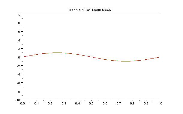
(a) $N=80$

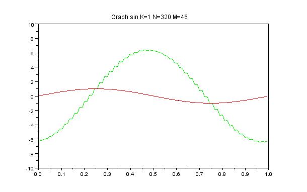
(b) $N=320$

Figure 2. Results for $N=80$ (left) and $N=320$ (right), using $P_{1}$ elements with $M=46$ in both cases. Instability appears on the right figure.

References

- [1] Y. Achdou and M. Falcone. A semi-Lagrangian scheme for mean curvature motion with nonlinear Neumann conditions. Interfaces Free Bound., 14(4):455–485, 2012.
- [2] O. Bokanowski and F. Bonnans. Semi-lagrangian schemes for second order equations. In preparation.
- [3] O. Bokanowski, Y. Cheng, and C.-W. Shu. Convergence of some Discontinuous Galerkin schemes for nonlinear Hamilton-Jacobi equations. To appear in Math. Comp.
- [4] F. Camilli and M. Falcone. An approximation scheme for the optimal control of diffusion processes. RAIRO Modél. Math. Anal. Numér., 29(1):97–122, 1995.
- [5] E. Carlini, R. Ferretti, and G. Russo. A weighted essentialy non oscillatory, large time-step scheme for Hamilton Jacobi equations. SIAM J. Sci. Comp., 27(3):1071–1091, 2005.
- [6] P. G. Ciarlet. Finite Element Method for Elliptic Problems. NorthHolland, Amsterdam, 1978.
- [7] B. Cockburn. Discontinuous Galerkin methods. ZAMM Z. Angew. Math. Mech., 83(11):731–754, 2003.
- [8] B. Cockburn and C.-W. Shu. Runge-kutta discontinuous galerkin methods for convection-dominated problems. Journal of Computational Physics, 223:398–415, 2007.
- [9] N. Crouseilles, M. Mehrenberger, and F. Vecil. Discontinuous Galerkin semi-Lagrangian method for Vlasov-Poisson. In CEMRACS’10 research achievements: numerical modeling of fusion, volume 32 of ESAIM Proc., pages 211–230. EDP Sci., Les Ulis, 2011.
- [10] K. Debrabant. Runge-Kutta methods for third order weak approximation of SDEs with multidimensional additive noise. BIT, 50(3):541–558, 2010.
- [11] K. Debrabant and E. R. Jakobsen. Semi-Lagrangian schemes for linear and fully non-linear diffusion equations. Math. Comp., 82(283):1433–1462, 2013.
- [12] F. Faà di Bruno. Note sur une nouvelle formule de calcul différentiel. Quarterly J. Pure Appl. Math., 1:359–360, 1857. (See also http://en.wikipedia.org/wiki/Faa_di_Bruno’s_formula).
- [13] M. Falcone and R. Ferretti. Convergence analysis for a class of high-order semi-Lagrangian advection schemes. SIAM J. Numer. Anal., 35(3):909–940 (electronic), 1998.
- [14] M. Falcone and R. Ferretti. Semi-Lagrangian approximation schemes for linear and Hamilton-Jacobi equations. Society for Industrial and Applied Mathematics (SIAM), Philadelphia, PA, 2014.
- [15] R. Ferretti. Convergence of semi-Lagrangian approximations to convex Hamilton-Jacobi equations under (very) large Courant numbers. SIAM J. Numer. Anal., 40(6):2240–2253 (2003), 2002.
- [16] R. Ferretti. A technique for high-order treatment of diffusion terms in semi-lagrangian schemes. Commun. Comput. Phys., 8:445–470, 2010.
- [17] R. Ferretti. On the relationship between semi-Lagrangian and Lagrange-Galerkin schemes. Numer. Math., 124(1):31–56, 2013.
- [18] E. Forest. Canonical integrators as tracking codes. (SSC-138), 1987.
- [19] E. Forest and R. Ruth. Fourth-order symplectic integration. Physica D: Nonlinear Phenomena, 43:105–117, 1990.
- [20] P. E. Kloeden and E. Platen. Numerical solution of stochastic differential equations, volume 23 of Applications of Mathematics (New York). Springer-Verlag, Berlin, 1992.
- [21] H. Kushner. Probability methods for approximations in stochastic control and for elliptic equations. Academic Press, New York, 1977. Mathematics in Science and Engineering, Vol. 129.
- [22] H. Kushner and P. Dupuis. Numerical methods for stochastic control problems in continuous time, volume 24 of Applications of mathematics. Springer, New York, 2001. Second edition.
- [23] P. Lesaint and P. A. Raviart. On a finite element method for solving the neutron transport equation. in Mathematical Aspects of Finite Elements in Partial Diffential Equations, pages 89–145, 1974.
- [24] J.-L. Menaldi. Some estimates for finite difference approximations. SIAM J. Control Optim., 27(3):579–607, 1989.
- [25] G. N. Milstein. Weak approximation of solutions of systems of stochastic differential equations. Theor. Prob. Appl., 30:750–766, 1986. (Transl. from Teor. Veroyatnost. i Primenen. 30 (1985), no. 4, 706–721.).
- [26] G. N. Milstein and M. V. Tretyakov. Numerical solution of the Dirichlet problem for nonlinear parabolic equations by a probabilistic approach. IMA J. Numer. Anal., 21(4):887–917, 2001.
- [27] K. W. Morton, A. Priestley, and E. Süli. Stability of the Lagrange-Galerkin method with nonexact integration. RAIRO Modél. Math. Anal. Numér., 22(4):625–653, 1988.
- [28] É. Pardoux and D. Talay. Discretization and simulation of stochastic differential equations. Acta Appl. Math., 3(1):23–47, 1985.
- [29] D. A. D. Pietro and A. Ern. Mathematical Aspects of Discontinuous Galerkin Methods, volume 69 of Mathematics & Applications. Springer-Verlag, Berlin, 2012.
- [30] E. Platen. Zur zeitdiskreten approximation von itoprozessen. Diss. B., 1984. IMath, Akad. der Wiss. Der DDR, Berlin.
- [31] J.-M. Qiu and C.-W. Shu. Positivity preserving semi-Lagrangian discontinuous Galerkin formulation: theoretical analysis and application to the Vlasov-Poisson system. J. Comput. Phys., 230(23):8386–8409, 2011.
- [32] M. Restelli, L. Bonaventura, and R. Sacco. A semi-Lagrangian discontinuous Galerkin method for scalar advection by incompressible flows. J. Comput. Phys., 216(1):195–215, 2006.
- [33] R. D. Richtmyer and K. W. Morton. Difference methods for initial-value problems. Second edition. Interscience Tracts in Pure and Applied Mathematics, No. 4. Interscience Publishers John Wiley & Sons, Inc., New York-London-Sydney, 1967.
- [34] J. A. Rossmanith and D. C. Seal. A positivity-preserving high-order semi-Lagrangian discontinuous Galerkin scheme for the Vlasov-Poisson equations. J. Comput. Phys., 230(16):6203–6232, 2011.
- [35] D. Ruth. A canonical integration technique. Technical report, 1983.
- [36] C. Steiner, M. Mehrenberger, and D. Bouche. A semi-Lagrangian discontinuous Galerkin approach. Technical Report hal-00852411, August 2013.
- [37] D. Talay. Efficient numerical schemes for the approximation of expectations of functionals of the solution of a SDE and applications. In Filtering and control of random processes (Paris, 1983), volume 61 of Lecture Notes in Control and Inform. Sci., pages 294–313. Springer, Berlin, 1984.
- [38] P. Wilmott, S. Howison, and J. Dewynne. The mathematics of financial derivatives. Cambridge University Press, Cambridge, 1995. A student introduction.
- [39] Y. Yang and C.-W. Shu. Analysis of optimal superconvergence of discontinuous Galerkin method for linear hyperbolic equations. SIAM J. Numer. Anal., 50(6):3110–3133, 2012.
- [40] H. Yoshida. Construction of higher order symplectic integrators. Physics Letters A, 150(5,6,7):262–268, 1990.
- [41] H. Yoshida. Recent progress in the theory and application of symplectic integrators. Celest. Mech. and Dyn. Astro., 56(1-2):27–43, 1993.