Transition Redshift: New constraints from parametric and nonparametric methods

Abstract

In this paper, we use the cosmokinematics approach to study the accelerated expansion of the Universe. This is a model independent approach and depends only on the assumption that the Universe is homogeneous and isotropic and is described by the FRW metric. We parametrize the deceleration parameter, $q(z)$, to constrain the transition redshift ($z_{t}$) at which the expansion of the Universe goes from a decelerating to an accelerating phase. We use three different parametrizations of $q(z)$ namely, $q_{\textnormal{\tiny{I}}}(z)=q_{\textnormal{\tiny{1}}}+q_{\textnormal{\tiny{2}}}z$, $q_{\textnormal{\tiny{II}}}(z)=q_{\textnormal{\tiny{3}}}+q_{\textnormal{\tiny{4}}}\ln(1+z)$ and $q_{\textnormal{\tiny{III}}}(z)=\frac{1}{2}+\frac{q_{\textnormal{\tiny{5}}}}{(1+z)^{2}}$. A joint analysis of the age of galaxies, strong lensing and supernovae Ia data indicates that the transition redshift is less than unity i.e. $z_{t}<1$. We also use a nonparametric approach (LOESS+SIMEX) to constrain $z_{t}$. This too gives $z_{t}<1$ which is consistent with the value obtained by the parametric approach.

^aDepartment of Physics $\&$ Astrophysics, University of Delhi, New Delhi 110007, India
        ^bDeen Dayal Upadhyaya College, University of Delhi, New Delhi 110015, India
       ^cDepartamento de Física Teórica e Experimental, UFRN, Campus Universitário,
         Natal, RN 59072-970, Brazil

  E-mail: nrani@physics.du.ac.in

1 Introduction

It is now widely accepted that we are living in a Universe which is accelerating at present [1, 2]. Measurements of distance moduli of Supernovae (SNe Ia) along with other independent observations such as results from the Planck satellite (Cosmic Microwave Background (CMB), Baryonic Acoustic Oscillations (BAO) ), etc. support this view [3, 4, 5]. However, the physics behind this late time cosmic acceleration is still a mystery. Cosmologists have come up with different models to solve this riddle [6]. Further, the discovery of high redshift SNe Ia provides strong evidence that the Universe was decelerating in the past [7]. Therefore, it is very important to find the epoch of transition from the slowing down to the speeding up of the expansion of the Universe.

Earlier Shapiro and Turner (2005) used both parametric and non-parametric methods to constrain the deceleration parameter, $q(z)$ and transition redshift, $z_{t}$ using SNe Ia data [8]. Melchiorri et. al (2007) also considered different dynamical dark energy models to put constraints on $z_{t}$ [9]. As expected, these constraints were model dependent. Further in 2007, Rapetti et al. developed a new kinematical method to study the dynamical history of the Universe [10]. By using the X-ray gas mass fraction measurements, they supported the transition of the Universe from a decelerated to an accelerated phase.

Many other authors have used different data sets such as Gamma Ray Bursts (GRBs), Hubble Observational Data $H(z)$, BAO, CMB, Galaxy Clusters , lookback time etc. to reconstruct $q(z)$ or to constrain the transition redshift [11, 12, 13, 14, 15, 16, 17, 18, 19, 20, 21, 22, 23]. Lima et al. (2012) have advocated many techniques that may constrain the transition redshift effectively in the future [24]. In a detailed study, Del Campo et al proposed three different $q(z)$ parametrizations and put constraints on the model parameters by using SNe Ia, $H(z)$, BAO/CMB data sets [25]. Recently, Vargas dos Santos et al. (2015) chose kink-like parametrizations of $q(z)$ and obtained constraints on the free model parameters especially the duration of the transition. They also used SNe Ia, BAO, CMB and H(z) data [26].

At present there is no well motivated theoretical model of the Universe which can explain all the aspects of this accelerated expansion. Hence it is reasonable to use a phenomenological approach. In this paper we study a popular cosmographic approach to characterize the properties of dark energy through the deceleration parameter. Here we also attempt to reconstruct $q(z)$ through a parametric method. This methodology has both advantages and disadvantages. One of the plus points of this technique is that it is independent of the matter-energy content of the Universe. The only assumption in this approach is that the Universe is homogeneous and isotropic on cosmic scales and the FRW metric is sufficient to describe the space-time of the Universe. The parametrization technique also helps to optimize future cosmological surveys. On the other hand, this formulation does not explain the real cause of the accelerated expansion. Further, the extracted value of the present deceleration parameter may be dependent on the assumed form of $q(z)$.

In this work we use three different parametrizations of $q(z)$ to constrain the transition redshift in a model independent manner. We also use information criteria to compare these models. As mentioned above, earlier work based on $q(z)$ parametrizations used SNe, $H(z)$, BAO, CMB etc. to study either the model parameters or the transition redshift. In this paper we highlight the importance of strong lensing data to study the “dynamic phase transition” in the universe when it switched from a decelerating to an accelerating phase. We further supplement this dataset with the age of galaxies and the recent data of SNe Ia (Joint Light Curve Analysis).

To check the consistency of our results, we also constrain $z_{t}$ using a nonparametric approach. Many nonparametric approaches like Principal Component Analysis (PCA), Gaussian Process (GP), Non Parametric Smoothing method (NPS) etc have been used in the literature to constrain cosmological parameters [27]. Here, we use the LOcally wEighted Scatterplot Smoothing method (LOESS). This method locates a smooth curve among the data points without having any information about the priors i.e. the functional form estimation is done using raw data only. For details of the method see [28, 29, 30]. This method does not consider the contribution of the observational errors. Therefore, in order to include the effects of errors in the analysis, LOESS is combined with SIMEX (SIMulation EXtrapolation method) [30].

The outline of the paper is as follows. In Section 2, we describe the parametric approach to put constraints on deceleration parameter ($q(z)$) and transition redshift ($z_{t}$). In Section 3 we adopt a nonparametric approach to constrain $z_{t}$. Discussion is presented in Section 4. Finally, Section 5 contains some concluding remarks.

2 Parametric Method

2.1 The Parametrizations of $q(z)$

The reconstructed form of the equation of state of dark energy ($\omega_{\tiny{de}}(z)$) is usually written as [31]

$$\omega_{\text{\tiny{de}}}(z)=\sum_{n=0}\omega_{n}x_{n}(z)$$ (1)

By analogy, we write the parametrized form of the deceleration parameter as

$$q(z)=\sum_{n=0}q_{n}x_{n}(z)$$ (2)

For different $x_{n}(z)$ we get different parametrizations of $q(z)$:

Redshift:         $x_{n}(z)=z^{n}$

Logarithmic:    $x_{n}(z)=[\textnormal{ln}(1+z)]^{n}$

Scale factor:     $x_{n}(z)=\left(\frac{1}{1+z}\right)^{2n}$

We use three different parametrizations of $q(z)$ corresponding to the above $x_{n}(z)$ [11, 32, 33].

$$q_{\textnormal{\tiny{I}}}(z)=q_{\textnormal{\tiny{1}}}+q_{\textnormal{\tiny{2}}}z$$ (3)

$$q_{\textnormal{\tiny{II}}}(z)=q_{\textnormal{\tiny{3}}}+q_{\textnormal{\tiny{4}}}\ln(1+z)$$ (4)

$$q_{\textnormal{\tiny{III}}}(z)=\frac{1}{2}+\frac{q_{\textnormal{\tiny{5}}}}{(1+z)^{2}}$$ (5)

The first parametrization is the Taylor series expansion of deceleration parameter around $z=0$ with $q_{\textnormal{\tiny{1}}}$ as the present value and $q_{\textnormal{\tiny{2}}}$ as the first derivative of $q(z)$ w.r.t. $z$. The second parametrization gives the present value of the deceleration parameter as $q_{\textnormal{\tiny{3}}}$ at $z=0$ while at higher redshifts it diverges. The third parametrization converges to $\frac{1}{2}$ as $z$ becomes large.

The Hubble parameter, $H(z)$ can be written in terms of $q(z)$ as

$$H(z)=H_{0}~{}\exp\left[\int\limits_{0}^{z}\frac{1+q(x)}{1+x}dx\right]$$ (6)

where $H_{0}$ is the present value of the Hubble constant.

The corresponding Hubble parameter for the above mentioned parametrizations can be expressed as-

$$H_{\textnormal{\tiny{I}}}(z,p)=H_{0}(1+z)^{1+q_{\textnormal{\tiny{1}}}-q_{\textnormal{\tiny{2}}}}~{}\exp(q_{\textnormal{\tiny{2}}}z)$$ (7)

$$H_{\textnormal{\tiny{II}}}(z,p)=H_{0}(1+z)^{1+q_{\textnormal{\tiny{3}}}}~{}\exp\left[\frac{q_{\textnormal{\tiny{4}}}}{2}[\ln(1+z)]^{2}\right]$$ (8)

$$H_{\textnormal{\tiny{III}}}(z,p)=H_{0}(1+z)^{\frac{3}{2}}~{}\exp\left[\frac{q_{\textnormal{\tiny{5}}}(z^{2}+2z)}{2(1+z)^{2}}\right]$$ (9)

Here $p$ represents the model parameters, i.e. the various $q_{i}^{\prime}s$.

2.2 Datasets and Method

2.2.1 Age of galaxies

We use two datasets of age of galaxies: Sample A and Sample B. Sample A consists of the age of $32$ passively evolving galaxies in the redshift range $0.117\leq z\leq 1.845$. This dataset is the collection of three subsamples [34].

The first subsample contains 10 early type field galaxies. The SPEED model is used to derive the age of these galaxies. It is assumed that stars in an elliptical galaxy have a single metallicity value which is an over-simplification. Further, the formation of stars in the single burst model may bias the age result as the formation of stars takes place at low redshift also. This problem can be rectified by considering only the old galaxies in each redshift bin. Jimenez et al. (2004) concluded from their study that the systematic errors associated with age of galaxies is not more than 10-15% even with these assumptions [35].

The second subsample consists of 20 old passive galaxies released by GDDS (Gemini Deep Deep Survey). The spectra obtained in this survey are of very high quality. For this subsample, McCarthy et al computed the synthetic spectra using the PEGASE.2 model and then compared the obtained spectra with the observed spectral energy distribution [36]. Simon et al. further reanalyzed this subsample using the SPEED model and obtained the age within 0.1 Gyr of the estimate of the GDDS collaboration. Finally, they emphasized that systematics are not a matter of concern for this subsample [34]. Dust depletion may also be a cause of systematic error, but this effect is again negligible.

The third subsample of sample A consists of two radio galaxies 53W091 and 53W069 [37, 38]. While deriving the age for these galaxies it was assumed that the large elliptical galaxy was formed in a single burst after which there was no star formation in it. This can cause over-estimation of age. However, the effect of the metallicity on the calculated age was found to be negligible. Following Samushia et al., we also use $12\%$ error in all the observed age data points[39].

We also work with another recent low redshift age dataset (Sample B) which consists of LRGs (Luminous Red Galaxies) selected from the SDSS DR7. This dataset consists of $12$ points in the redshift range $0.05<z<0.4$ [40]. The full spectrum fitting method is used to obtain the age of these galaxies by using the single population synthesis model (GalexEV/SteLib). The reason for using the combined spectrum is to improve the signal to noise ratio and to reduce contamination. Liu et al argue that the recent star formation in the galactic center of massive galaxies may systematically underestimate the obtained mean age at $z\leq 0.4$  [40]. But this bias is not very significant for galaxies with a large velocity dispersion. Following this criterion, we also prefer to use subsample IV of the data (Liu G., private communication, 2015).

We use the minimum chi-square technique to find the best fit model parameters.

$$\chi^{2}=\sum_{i=1}^{n_{1}}\frac{[t^{th}(z_{i},p)-\tau-t^{obs}(z_{i})]^{2}}{\sigma_{i}^{2}}$$

where $n_{1}$ is the number of data points used in the sample, $t^{th}(z_{i},p)$ is the theoretical age of the galaxy, $\tau$ is the delay factor or incubation time, $t^{obs}$ is the measured current age of the galaxy and $\sigma_{i}$ is the uncertainty in the observed age.

The theoretical expressions for the ages of galaxies ($t^{\tiny{th}}(z_{i},p)$) corresponding to the three parametrizations are as follows:

$$t_{\textnormal{\tiny{I}}}(z,p)=H_{0}^{-1}\int\limits_{0}^{\frac{1}{1+z}}x^{q_{\textnormal{\tiny{1}}}-q_{\textnormal{\tiny{2}}}}~{}~{}\exp\left[-q_{\textnormal{\tiny{2}}}\left(\frac{1-x}{x}\right)\right]dx$$ (10)

$$t_{\textnormal{\tiny{II}}}(z,p)=H_{0}^{-1}\int\limits_{0}^{\frac{1}{1+z}}x^{q_{\textnormal{\tiny{3}}}}\exp\left[-\frac{q_{\textnormal{\tiny{4}}}}{2}\left[\ln~{}\left(\frac{1}{x}\right)\right]^{2}\right]dx$$ (11)

$$t_{\textnormal{\tiny{III}}}(z,p)=H_{0}^{-1}\int\limits_{0}^{{\frac{1}{1+z}}}x^{\frac{1}{2}}~{}\exp\left[-\frac{q_{\textnormal{\tiny{5}}}}{2}(1-x^{2})\right]dx$$ (12)

Here $p$ represents the model parameters, i.e. the various $q_{i}^{\prime}s$.

In an earlier work, marginalization was done over the delay factor only and $H_{0}$ was kept fixed for the kinematic approach [11]. The recent value of $H_{0}$ determined by SNe and Mega-masers and also through a combination of data including the age of old galaxies at intermediate redshift are $73.8\pm 2.4~{}{\textnormal{K}ms^{-1}Mpc^{-1}}$ and $74.1\pm 2.2~{}{\textnormal{K}ms^{-1}Mpc^{-1}}$ respectively [41, 42]. However, the Planck results suggest $H_{0}=67.8\pm 0.9~{}{\textnormal{K}ms^{-1}Mpc^{-1}}$ [43]. Therefore instead of choosing fixed value of $H_{0}$, we minimized $\chi^{2}$ w.r.t. $H_{0}$ in order to take care care of this discrepancy. We find that minimization and marginalization are equivalent in our case.

$$\chi^{2}=A+C\tau^{2}+2B\tau$$ (13)

So we first minimize chi-square over the delay factor$(\tau)$. The minimum value of chi-square is

$$\tilde{\chi}^{2}=A-\frac{B^{2}}{C}$$ (14)

where

$$A=\sum_{i=1}^{n_{1}}\frac{(t^{th}(z_{i},p)-t^{obs}(z_{i}))^{2}}{\sigma_{i}^{2}},~{}~{}~{}~{}B=\sum_{i=1}^{n_{1}}\frac{(t^{th}(z_{i},p)-t^{obs}(z_{i}))}{\sigma_{i}^{2}},~{}~{}~{}~{}C=\sum_{i=1}^{n_{1}}\frac{1}{\sigma_{i}^{2}}$$

$\tilde{\chi}^{2}$ is again minimized over $H_{0}$

$$\tilde{\tilde{\chi}}=\frac{d\tilde{\chi}^{2}}{dH_{0}}=\frac{dA}{dH_{0}}-\frac{2B}{C}\frac{dB}{dH_{0}}$$ (15)

$$\textnormal{where}~{}~{}~{}~{}~{}\frac{dA}{dH_{0}}=\frac{-2D}{H_{0}^{3}}+\frac{2G}{H_{0}^{2}}$$

$$\textnormal{and}~{}~{}~{}\frac{dB}{dH_{0}}=-\frac{E}{H_{0}^{2}}$$

Putting the values of $\frac{dA}{dH_{0}}$ and $\frac{dB}{dH_{0}}$ in Equation (15) and equating to $0$, we get

$$\frac{1}{H_{0}}=\frac{-JE+GC}{-E^{2}+CD}$$

where

$$M=\sum_{i=1}^{n_{1}}\frac{[t_{obs}(z_{i})]^{2}}{\sigma_{i}^{2}},~{}~{}~{}~{}J=\sum_{i=1}^{n_{1}}\frac{t_{obs}(z_{i})}{\sigma_{i}^{2}},~{}~{}~{}~{}G=\sum_{i=1}^{n_{1}}\frac{\Delta(z_{i},p)t_{obs}(z_{i})}{\sigma_{i}^{2}}$$

$$E=\sum_{i=1}^{n_{1}}\frac{\Delta(z_{i},p)}{\sigma_{i}^{2}},~{}~{}~{}~{}D=\sum_{i=1}^{n_{1}}\frac{[\Delta(z_{i},p)]^{2}}{\sigma_{i}^{2}},~{}~{}~{}~{}\Delta(z_{i},p)=\frac{t^{\tiny{th}}(z_{i},p)}{H_{0}^{-1}}$$

The final chi-square obtained after minimizing over both the delay factor and the Hubble parameter is given by

$$\tilde{\tilde{\chi}}_{age}^{2}=M-\frac{J^{2}}{C}-\frac{(GC-JE)^{2}}{C(E^{2}-CD)}$$ (16)

2.2.2 Strong lensing

When light passes near matter, it bends due to the gravitational field. The same phenomenon occurs if there is a galaxy or galaxy cluster (lens) in the path of light coming from a bright object (quasar) usually termed as the source. If the source, lens and the observer are placed in such a way that all three lie in the same line of sight then a ring-like structure, called an Einstein ring, is formed and the phenomenon is called strong lensing (SL). Two or more images can form in strong lensing (for details see [44]).

The phenomenon of strong lensing can be used to constrain cosmological parameters. If we assume that the Singular Isothermal Sphere (SIS) or Singular Isothermal Ellipsoid (SIE) model can be used to represent the gravitational lens, then the radius of the Einstein ring is [45, 46, 47, 48]

$$\theta_{E}=4\pi\frac{\sigma^{2}_{\textnormal{\tiny{SIS}}}}{c^{2}}\frac{D_{ls}}{D_{os}}$$ (17)

Here $\theta_{E}$ is the radius of the Einstein ring, $D_{ls}$ is the angular diameter distance between the lens and the source, $D_{os}$ is the angular diameter distance between the observer and the source and $\sigma_{\textnormal{\tiny{SIS}}}$ is the velocity dispersion of the mass distribution of the lens.

We define the ratio of the measured angular diameter distances, i.e. $D_{ls}$ and $D_{os}$, as $\mathcal{D}^{obs}$:

$$\mathcal{D}^{obs}\equiv\frac{D_{ls}}{D_{os}}=\frac{c^{2}\theta_{E}}{4\pi\sigma_{\textnormal{\tiny{SIS}}}^{2}}$$ (18)

We select a subsample from the Sloan Lens ACS (SLACS) and Lens Structure and Dynamics survey (LSD). This subsample consists of $70$ data points in which lensing occurs due to galaxies while for the rest 10 lensing occurs due to clusters. In treating lensing due to clusters, several assumptions are commonly made like the whole gas inside is at same temperature, the gas pressure and gravity of the relaxed cluster balance each other according to hydrostatic equilibrium and the cluster is spherically symmetric. These assumptions may over-simplify the results and hence we do not include cluster data in our analysis. We also do not consider the four-image lens systems as the SIS lens model produces two images only. Finally we are left with a subsample which consists of $36$ data points. It is important to note that though the range $0\leq\mathcal{D}^{obs}\leq 1$ is the only physically meaningful one as $D_{ls}$ should always be smaller than $D_{os}$, we have also included points with $\mathcal{D}^{obs}>1$ since this is within 1$\sigma$. The redshift ranges of the lens and the source are $0.106\leq z_{l}\leq 1.004$ and $0.1965\leq z_{s}\leq 3.9$ respectively (for details see [45]).

To constrain the best fit model parameter, chi-square is written as

$$\chi_{SL}^{2}(p)=\sum_{i=1}^{n_{2}}\frac{(\mathcal{D}_{i}^{th}(p)-\mathcal{D}_{i}^{obs})^{2}}{\sigma_{\mathcal{D}^{obs}}^{2}}$$ (19)

where $n_{2}=36$ and $\sigma_{\mathcal{D}^{obs}}$ is the uncertainty in $\mathcal{D}^{obs}$.

The corresponding theoretical quantity $\mathcal{D}^{th}$ can be written as

$$\mathcal{D}^{th}(z_{l},z_{s};p)=\frac{D_{ls}^{th}}{D_{os}^{th}}=\frac{D_{A}(z_{l},z_{s};p)}{D_{A}(0,z_{s};p)}$$ (20)

In flat Friedmann-Robertson-Walker (FRW) cosmology, the angular diameter distance is

$$D_{A}(z_{l},z_{s};p)=\frac{1}{(1+z_{s})}\frac{c}{H_{0}}\int\limits_{z_{l}}^{z_{s}}\frac{dx}{E(x;p)}$$ (21)

$$D_{A}(0,z_{s};p)=\frac{1}{(1+z_{s})}\frac{c}{H_{0}}\int\limits_{0}^{z_{s}}\frac{dx}{E(x;p)}$$ (22)

$$E(x;p)=\frac{H(x;p)}{H_{0}}$$ (23)

In this method, the cosmological model enters through the ratio of the two angular diameter distances and so it is completely independent of the Hubble constant.

2.2.3 Supernova Ia

We use the latest Supernova Ia data which consists of $740$ data points [49]. This includes data from low redshift ($z<0.1$), SDSS-II ($0.05<z<0.4$) and SNLS 3 year ($0.2<z<1.0$) supernova samples. It is assumed that the supernova will have the same intrinsic luminosity at all redshifts provided they have identical colours, the same galactic environment and shape. This assumption is expressed through the distance estimator which can be written as [50]

$$\mu_{obs}(\alpha,\beta;M)=m^{*}_{B}-M+\alpha~{}X_{1}-\beta~{}C$$

Here $m^{*}_{B}$ is the rest-frame B band peak magnitude, and $\alpha$, $\beta$ and $M$ are the nuisance parameters. $X_{1}$ and $C$ describe the stretching of the light curve and colour at maximum brightness respectively.

The chi-square for the supernova analysis is written as

$$\chi^{2}_{\tiny{JLA}}(\mu_{0},M;p_{th},p_{obs})=\sum_{i=1}^{n_{3}}\frac{[\mu_{th}(z_{i};p_{th},\mu_{0})-\mu_{obs}(p_{obs};M)]^{2}}{\sigma_{\mu}^{2}}$$

where $n_{3}=740$, $p_{th}$ represents the model parameters and $p_{obs}$ are the nuisance parameters present in $\mu_{obs}$, i.e. $\alpha$ and $\beta$. We fix the values of $\alpha$ and $\beta$ according to the $\Lambda$CDM model as $0.14$ and $3.14$ respectively while we minimize over the parameters $M$ and $H_{0}$ [50].

Chi-square obtained after minimization over $M$ and $H_{0}$ is

$$\tilde{\chi}_{JLA}^{2}(p_{th},p_{obs})=A^{\prime}-\frac{B^{\prime 2}}{C^{\prime}}$$

$$A^{\prime}=\sum_{i=1}^{n_{3}}\frac{[\mu_{th}(z_{i};p_{th})-\mu_{obs}(p_{obs})]^{2}}{\sigma_{\mu}^{2}}$$

$$B^{\prime}=\sum_{i=1}^{n_{3}}\frac{[\mu_{th}(z_{i};p_{th})-\mu_{obs}(p_{obs})]}{\sigma_{\mu}^{2}}$$

$$C^{\prime}=\sum_{i=1}^{n_{3}}\frac{1}{\sigma_{\mu}^{2}}$$

$$\mu_{th}=5log_{10}(d_{l})+\mu_{0}$$

where $d_{l}$ is the Hubble-free luminosity distance and

$$\mu_{0}=5log_{10}(c/H_{0})+25$$

The combined chi-square is the sum of chi-squares obtained from all three datasets i.e.

$$\chi_{tot}^{2}=\tilde{\tilde{\chi}}_{age}^{2}+\chi^{2}_{\tiny{SL}}+\tilde{\chi}^{2}_{\tiny{JLA}}$$ (24)

2.3 Results

We parameterize the deceleration parameter with a two-parameter function ($q_{I}(z),q_{II}(z)$) and a one-parameter function ($q_{III}(z)$) to understand the expansion history of the Universe.. By fitting these functions to the combined set of Age, SL and SNe Ia data, we get the constraints described below.

•  Parametrization I   $q_{\textnormal{\tiny{I}}}(z)=q_{\textnormal{\tiny{1}}}+q_{\textnormal{\tiny{2}}}z$

Figure 1 shows $68.3\%$, $95.4\%$ and $99.7\%$ confidence level ellipses in the model parameter plane for the combined (Age+SL+JLA) dataset. Figure 2 shows the evolution of $q(z)$ w.r.t. $z$ with $1\sigma$, $2\sigma$ and $3\sigma$ errors.

The best fit parameter values for this parametrization are tabulated in Table 1. The value of $z_{t}$ from the strong lensing data is relatively large but combination of the three datasets (Age+SL+JLA) lowers it to a value which matches with other observations. The value of $q_{\textnormal{\tiny{I}}}(0)$ for the combined analysis is $-0.52$.

Table 1: Values of best fit parameters for $q_{\textnormal{\tiny{I}}}(z)$

Dateset	Age (Sample A)	Age (Sample B)	SL	JLA	Age(A+B)+SL+JLA
$q_{\textnormal{\tiny{1}}}$	-1.68	-0.052	-0.85	-0.57	-0.52
$q_{\textnormal{\tiny{2}}}$	1.55	0.54	0.23	0.74	0.53
$q_{\textnormal{\tiny{I}}}(0)$	-1.68	-0.052	-0.85	-0.57	-0.52
$\chi^{2}$	12.28	8.60	64.71	624.82	842.31
$\chi^{2}_{\nu}$	0.41	0.86	1.9	0.85	1.03
$z_{t}$	1.08	0.10	3.70	0.77	0.98
FoM	0.71	0.007	4.62	84.52	99.75

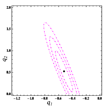
Figure 1: 1$\sigma$, 2$\sigma$ and 3$\sigma$ confidence level contours of chi-square in the $q_{\textnormal{\tiny{1}}}-q_{\textnormal{\tiny{2}}}$ plane for the combined datasets (Age+SL+JLA). The black dot shows the best fit value of the parameters.

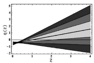
Figure 2: The variation of $q_{I}(z)$ vs $z$ with 1$\sigma$, 2$\sigma$ and 3$\sigma$ confidence regions. The thick black line is the best fit line. The horizontal line represents $q(z)=0$.

• Parametrization II:  $q_{\textnormal{\tiny{II}}}(z)=q_{\textnormal{\tiny{3}}}+q_{\textnormal{\tiny{4}}}\ln(1+z)$

For the combined dataset, the 1$\sigma$, 2$\sigma$ and 3$\sigma$ confidence contours in the $q_{\textnormal{\tiny{3}}}-q_{\textnormal{\tiny{4}}}$ plane are plotted in Figure 3. The value of $z_{t}$ obtained from the strong lensing data is once again on the high side, but by combining the strong lensing, age and JLA data, we get a value of $z_{t}$ which is consistent with other observations such as $H(z)$ etc. within 3$\sigma$ level. The value of $q_{\textnormal{\tiny{II}}}(0)$ for the combined dataset is $-0.56$. The best fit values of the model parameters are given in Table 2.

Table 2: Values of best fit parameters for $q_{\textnormal{\tiny{II}}}(z)$

Dataset	Age (Sample A)	Age (Sample B)	SL	JLA	Age(A+B)+SL+JLA
$q_{\textnormal{\tiny{3}}}$	-1.88	-0.04	-0.84	-0.61	-0.56
$q_{\textnormal{\tiny{4}}}$	2.54	0.54	0.30	1.02	0.83
$q_{\textnormal{\tiny{II}}}(0)$	-1.88	-0.04	-0.84	-0.61	-0.56
$\chi^{2}$	12.35	8.60	64.76	624.49	841.38
$\chi^{2}_{\nu}$	0.41	0.86	1.9	0.85	1.03
$z_{t}$	1.09	0.08	15.44	0.82	0.96
$FoM$	0.39	0.006	2.58	65.32	73.90

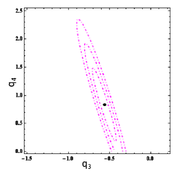
Figure 3: $1\sigma$, $2\sigma$ and $3\sigma$ confidence level ellipse for the combined observations. Black dot represents the best fit value of the model parameters.

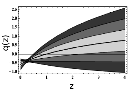
Figure 4: Evolution of $q_{II}(z)$ with $z$. The filled regions are the 1$\sigma$, 2$\sigma$ and 3$\sigma$ confidence level regions respectively. The thick black line is the best fit line. The horizontal line represents $q(z)=0$.

•  Parametrization III:  $q_{\textnormal{\tiny{III}}}(z)=\frac{1}{2}+\frac{q_{\textnormal{\tiny{5}}}}{(1+z)^{2}}$

The value of best fit parameters for different datasets are tabulated in Table 3. $q_{\textnormal{\tiny{III}}}(0)$ for the joint analysis is $-0.8$. Figures 5 and 6 show the variation of the chi-square with model parameters and the evolution of the deceleration parameter with redshift respectively.

Table 3: Values of best fit parameters for $q_{\textnormal{\tiny{III}}}(z)$

Dataset	Age (Sample A)	Age (Sample B)	SL	JLA	Age(A+B)+SL+JLA
$q_{\textnormal{\tiny{5}}}$	-2.58	-0.57	-2.14	-1.3	-1.30
$q_{\textnormal{\tiny{III}}}(0)$	-2.08	-0.07	-1.64	-0.8	-0.80
$\chi^{2}$	12.47	8.67	66.13	625.23	841.62
$\chi^{2}_{\nu}$	0.42	0.86	1.9	0.85	1.03
$z_{t}$	1.27	0.07	1.07	0.61	0.60

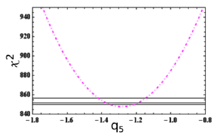
Figure 5: Chi-square vs model parameter variation is shown by the Dot-Dashed line for the combined observations. Black horizontal lines are the 1$\sigma$, 2$\sigma$ and 3$\sigma$ lines.

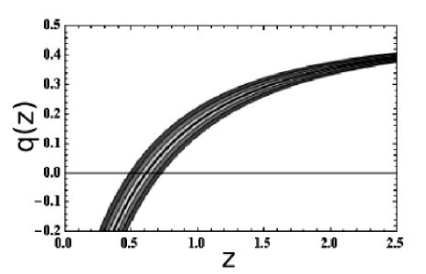
Figure 6: The evolution of $q_{III}(z)$ with $z$. The $1\sigma$, $2\sigma$ and $3\sigma$ confidence regions are shown by the filled regions. The thick black line is the best fit line. The horizontal line is the line corresponding to $q(z)=0$

2.4 Information Criteria

Information criteria are used to rank different models that are available to describe a given dataset. We use the Akaike Information Criterion (AIC) and the Bayesian Information Criterion (BIC). For details see [51, 52, 53]

$$\textnormal{AIC}=\chi^{2}+2P$$

$$\textnormal{BIC}=\chi^{2}+2P\textnormal{ln}d$$

where $P$ and $d$ are the number of model parameters and data points in the dataset respectively. $\chi^{2}$ is the minimum value of chi square. If $d/P<40$, it is good to use the corrected Akaike Information Criterion ($\textnormal{AIC}_{c}$) [54].

$$\textnormal{AIC}_{c}=\textnormal{AIC}+\frac{2P(P+1)}{(d-P-1)}$$

In our work $d/P>40$ and so we calculate AIC for all three parametrizations. We also calculate BIC. To compare the models, we calculate the differences given by $\Delta$AIC and $\Delta$BIC.

$$\Delta\textnormal{AIC}=\textnormal{AIC}_{j}-\textnormal{AIC}_{m}$$

$$\Delta\textnormal{BIC}=\textnormal{BIC}_{j}-\textnormal{BIC}_{m}$$

$\textnormal{AIC}_{m}$ and $\textnormal{BIC}_{m}$ are the minimum value of AIC and BIC respectively. If more than one model fits the observations equally, then the value of AIC and BIC will be minimum for the model having the minimum number of model parameters.

•  Summary of Information Criteria Results

The results for different models using the information criteria is given in Table 4.

Table 4: Information Criteria results for Age, SL and JLA data

Model	$P$	$\Delta$ BIC	$\Delta\textnormal{AIC}$
$q_{\tiny{I}}(z)$	2	14.11	4.70
$q_{\tiny{II}}(z)$	2	13.18	3.77
$q_{\tiny{III}}(z)$	1	0.0	0.0

$\bullet$ We also use the Figure of Merit (FoM) tool to quantify the robustness of the constraints obtained. For two parameters, FoM is defined as the inverse of $95\%$ confidence limit area. Tighter constraints in the parametric space give large values of FoM’s.

3 Nonparametric Method

3.1 Hubble Data

For this, we use recent Hubble data which includes $30$ data points. The redshifts of the passively evolving galaxies are known with high accuracy. So these galaxies can be used as chronometers and can provide the direct measurement of the $H(z)$. This is known as the differential age approach and 23 data points in this dataset are measured using this approach. The second way to measure $H(z)$ is by the clustering of the galaxies. In this method, $H(z)$ measurement is done by using the peak position of the BAO in the radial direction as the standard ruler. This approach is called clustering. Seven measurements of $H(z)$ are done by clustering. The complete dataset is taken from Yun Chen et al. [48]

3.2 Method

Non parametric method includes the study of the neighbourhood points of the focal point. For this we need to calculate the smoothing parameter or span $(s)$. This parameter tells us about the proportion of observations to be used in the local regression. $s$ ranges from $0$ to $1$. To find the appropriate value of $s$, we use the cross-validation method [30]. In this method, the cross-validation function $(CV)$ is defined as

$$CV(s)=\frac{1}{n}\sum_{i}(h(z_{i})-\hat{h}(z_{-i}))^{2}$$ (25)

where $n$ is the number of data points used in LOESS, $h(z_{i})$ are the data points of the original data, $\hat{h}(z_{-i})$ are the fitted values obtained after omitting the $i^{th}$ observation from the local regression method at the point of interest i.e. $z_{i,0}$. $CV$ is calculated for different $s$ i.e. from 0.2 to 1. The value of $s$ which minimizes $CV$ is the best smoothing parameter for the particular data set. For the data set we use, $s=0.92$ is the best value.

The number of data points that we will use in LOESS can be calculated using the relation

$$n=N.s$$ (26)

where $N$ is the total number of data points. In the data set we use, $N=30$ and $s=0.92$ so $n=27$.

The next step of the method is the estimation of kernel in such a way that the points closer to the focal point ($z_{i,0}$) get more weight then the farther points. This is because the points which are closer to the focal point are more correlated and so will affect the estimation of $\hat{h}(z_{i})$ more than the farther points. The weight or kernel function can be calculated using the following tricube function

$$w_{ij}=\left\{\begin{array}[]{l l}(1-u_{ij}^{3})^{3}&\quad{\textnormal{for}~{}~{}|u_{ij}|<1}\\ 0&\quad\text{otherwise}\end{array}\right.$$ (27)

where

$$u_{ij}=\frac{(z_{j}-z_{i,0})}{\Delta}$$ (28)

$\Delta$ is the maximum difference between the focal point and the last ($j^{th}$) element of its window i.e. max$|z_{j}-z_{i,0}|$.

To calculate the value of reconstructed $h(z)$ i.e. $\hat{h}(z_{i})$, we define chi-square as

$$\chi^{2}=\sum_{i=1}^{n}w_{ij}(h(z_{i})-a-(b*z_{i}))^{2}$$ (29)

The value of $[a+(b*z_{i})]$ which minimizes chi-square gives the value of $\hat{h}(z_{i})$. This process is repeated for all data points to find the reconstructed value corresponding to all redshifts given in the real data.

3.3 Results

The $CV$ versus $s$ plot is shown in Figure 7. This shows that the smoothing parameter value which minimizes the cross validation function is $0.92$.

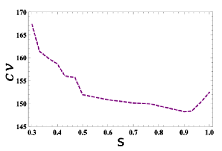
Figure 7: CV vs s plot for the Hubble data

Figure 8 shows the variation of $H(z)/(1+z)$ with $z$. The scattered points are the values of $H(z)/(1+z)$ from the data with error bars.The blue line represents the reconstructed values of $H(z)/(1+z)$ using the LOESS method. In the LOESS method observational errors are not taken into account. This can be done using the SIMEX. The results of using LOESS with SIMEX is shown by the orange line in Figure 8. The detail of SIMEX are given in [30]. It is clear from the plot that the transition from decelerated expansion to accelerated expansion occurs at $z_{t}\sim 0.7$. For reference we plot the $H(z)/(1+z)$ for $\Lambda$CDM model (green line) which gives $z_{t}\sim 0.6$.

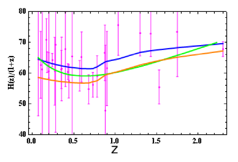
Figure 8: Variation of $H(z)/(1+z)$ with $z$; the blue line corresponds to the reconstructed values through LOESS, the orange line shows reconstructed values from LOESS+SIMEX and the green line is for $\Lambda$CDM model.

4 Discussion

In the present analysis we use a sample of age data (passively evolving galaxies+LRGs) which has $44$ points and is therefore larger than the data used earlier. As pointed out earlier, Jimenez et al. (2004) showed that the uncertainties associated with the age data may not be more than $10-15\%$ [35]. Recently, Jun Jie Wei et al. analysed the data with $24\%$ uncertainty in the observed age of passively evolving galaxies in order to take care of some of the unknown systematics which are not sufficiently understood [55]. As expected, the constraints obtained on the model parameters were weaker. Wei et al. also relaxed the assumption of a uniform delay factor for all galaxies. Instead they considered the case in which the delay factor is distributed through a Gaussian and a Top Hat distribution. They conclude that the delay factor distribution does not affect the result significantly. In the present work, we minimize both the effect of delay factor and Hubble parameter analytically, something we believe has not been addressed completely in the past.

Strong gravitational lensing is another important tool used in this work to constrain the transition redshift. Recent work done by different groups has made this probe more popular to constrain the cosmological parameters [45, 56, 57, 58]. But there are many systematic issues with this method. The three important uncertainties associated with this method are the unknown mass distribution of the galaxies, stellar velocity dispersion and the line of sight mass contamination. Further, the data for lensing is drawn from different surveys which may also cause a systematic error.

As the true mass profile of the galaxies is not known, various models have been proposed in the literature. But due to the simplicity, most frequently used are the SIS (Singular Isothermal Sphere) and SIE (Singular Isothermal Ellipsoid) models. The advantage of considering the SIS model is that, to a first approximation, it describes the average properties of the galaxies quiet accurately. However, real galaxies show some deviation from the assumed symmetry. Models including ellipticity provide a better description of mass distribution but they need a comparatively large number of parameters.

As mentioned earlier, the total density distribution of the lenses is described by the SIS model (stellar and dark matter halo). In principle, the velocity dispersion of the stellar component might be different from that of the dark component. This fact is supported by X-ray properties of late elliptical galaxies. Treu et al. (2006), after analysing the large sample of lenses of SLACS survey [59], noticed that the average ratio of $\sigma_{0}$ and $\sigma_{SIS}$ (for the total mass) is very close to unity. This result suggests that some unknown nexus exists between the stellar and dark matter halo which is sometime referred to as the ”bulge halo conspiracy”. In practice, $\sigma_{0}$ and $\sigma_{SIS}$ are related as

$$\sigma_{SIS}=f_{\tiny{E}}\sigma_{0}$$

Here $f_{E}$ is a free parameter which incorporates the uncertainties like the error introduced in $\theta_{E}$ due to the SIS assumption, the rms error between the observed velocity dispersion and model velocity dispersion etc. In literature, $f_{E}$ has been treated in a variety of ways. Melia et al. for instance, kept it as a free parameter [57]. Wang and Xu present a new method which completely eliminates the uncertainty appearing due to $f_{E}$ [60]. Van de Ven et al have found that $\sqrt{0.8}<f_{E}<\sqrt{1.2}$ [61]. In this work we assume $f_{E}=1$.

The third systematic is due to line of sight mass contamination [56, 62, 63]. In the present work, lenses are assumed to be isolated. In principle the line of sight density fluctuations can affect the lens model also. Bar-kana showed that large scale structure (LSS) changes the angular diameter distance at a given redshift [64]. This shows that if the effect of LSS, is not included while reconstructing the lens, it may lead to incorrect conclusions. This effect dominates when the source and the lens are at large redshifts. Keeton et al claim that external shear perturbation is small due to LSS so its effect on gravitational lenses can be neglected [65]. A larger dataset for strong lensing may help to get rid of this effect.

The total uncertainty present in $\mathcal{D}^{obs}(\sigma_{0},f_{E},\theta_{E})$ is calculated by using the propagation equation. The uncertainty both in the Einstein radius $\theta_{E}$ and the velocity dispersion $\sigma_{0}$ are $\sim 5\%$ each [66]. The error in $f_{E}$ is nearly $6\%$ [57, 59, 61]. So the total error in $\mathcal{D}^{obs}$ comes out to be approximately $16\%$ .

5 Conclusions

More than four decades ago, Allan Sandage (1970) argued that we need a precise measurement of the Hubble constant ($H_{0}$) and the deceleration parameter $q(z)$ to distinguish between various cosmological models [67]. But with the progress in the cosmological observations, it is believed that we may require more than two numbers to understand the expansion history of the universe [68]. In this regard, the reconstruction of $q(z)$ and the study of the transition redshift are very important in describing the evolution history of the universe.

One of the objective of this work is to include strong lensing (SL) data for the reconstruction of $q(z)$ through a parametric approach. There are many advantages of using SL data in the form of distance ratio. Firstly, this ratio is independent of the Hubble parameter. Secondly, this data can lift the degeneracies in the determination of the constraints obtained from the other observations. Finally, this method does not depend upon the evolutionary effect of the sources and is also immune to dust absorption. In contrast to the SL data, the constraints obtained from the age data depend upon the Hubble parameter. Therefore we have minimized the $\chi^{2}$ w.r.t. $H_{0}$ and the delay factor analytically, which was not addressed completely in the past [11].

The constraints obtained on the transition redshift by using strong lensing, age of the galaxies and recent SNe Ia data through a parametric approach are as follows:

$1.$ All the three $q(z)$ parametrizations are consistent with an accelerating universe at the present epoch and the best fit value of $z_{t}$ is less than $1$.

$2.$ Within $3\sigma$ confidence level, both the present values of the deceleration parameter and the transition redshift are in concordance with the constraints obtained from the other observations such as H(z), BAO, Clusters etc.

$3.$ The evolution of the deceleration parameter w.r.t. the redshift shows that there is no slowing down of the present cosmic acceleration as reported earlier [69, 70].

$4.$ We observe the tension between the results obtained from the high redshift ( Sample A) and the low redshift age data ( Sample B). This inconsistency disappears when it is combined with other datasets.

$5.$ The present value of $q(z)$ and $z_{t}$ obtained from these parametrizations ($q_{I},q_{II}$) have large error bars at high redshift. This may be due to lack of data points and more importantly the uncertainties associated with the lensing data set. The present strong lensing data is not precise enough to constrain the model parameters tightly. Therefore, we use the combination of age, strong lensing and SNe Ia data. These observations have different restrictive powers in the parametric space. Hence, it is always better to use complementary tools to put constraints on the model parameter. This also helps to break the degeneracy inherent in the parametric space. With the addition of age data and SNe Ia data, the constraints on the parameters improve and become consistent with the $\Lambda$CDM model.

$6.$ We use two information criteria (AIC & BIC) for selecting the best parameterization. $\Delta$BIC greater than $6$ is considered as strong evidence against the model with the higher BIC [54]. The rule remains same for $\Delta$AIC. In our calculation, $\Delta$AIC and $\Delta$BIC are minimum for the third parametrization as expected. The value of $\Delta$BIC is greater than $6$ for the first and second parametrizations, which indicates a positive evidence against these models. We believe that the IC analysis favours the third parametrization.

In order to obtain the effective constraints using SL data, one must control the associated systematics. One very important parameter linked with SL measurements is the observed velocity dispersion (${D_{ls}/D_{os}}\propto\sigma^{2}$). As reported by Schwab et al. [71], the actual velocity dispersion is luminosity weighted along the line of sight and also over the spectrometer aperture. In addition to all these factors, one should also take care of the radial and tangential component of velocity dispersion. After including the above factors in the analysis, $\mathcal{D}^{obs}$ is replaced by [72]

$$N(\alpha,\beta,\gamma,\delta){\theta_{E}^{\alpha-1}\over{4\pi\sigma_{0}^{2}}}$$

This modified ratio takes care of the anisotropy present in the velocity dispersion as well as other lens parameters.

As $\mathcal{D}^{obs}$ is dependent on $\sigma_{0},N(\alpha,\beta,\gamma,\delta)$ and $\theta_{E}$, it is crucial to check the sensitivity of these parameters on the $\mathcal{D}^{obs}$. If we substitute the mean values of these parameters, we find that the value of $\mathcal{D}^{obs}$ gets reduced by around $12\%$. What is more surprising is that this new data set of reduced $\mathcal{D}^{obs}$ leads to a universe which is decelerating at present, something which is not supported by observations. This leads us to conclude that our understanding of the lens quantities needs to improve further.

The point we want to highlight is that the determination of lens parameters as well as the observed quantities in the SL data are very crucial. Small changes in the lens parameters may change the result completely. Therefore a better understanding of the assumptions and the systematics associated with the lens parameters must be addressed.

The obtained constraints are limited by the quantity and the quality of the data for strong lensing. Nevertheless, the obtained results are meant to highlight the importance of strong lensing as well as the updated age data which gives an independent estimate of the cosmological parameters. At present the known gravitational lenses are of the order $\sim 10^{2}$. It is expected that next generation space telescopes such as Euclid will observe $\sim 10^{5}$ strong galaxy-galaxy gravitational lenses. So in the near future, we can expect that the enhanced data sets will allow us to put tighter constraints on the cosmological parameters [73]. Similarly it is also expected that future surveys such as BOSS will observe a large number of quiescent massive LRGs and hence more accurate age-redshift data of galaxies will be obtained [74]. This may further reduce the systematic uncertainties associated with age data.

The constraints obtained from the nonparametric approach are summarized as follows:

$7.$ We have applied a nonparametric method (LOESS) to constrain $z_{t}$ by using the Hubble data only because this technique can reconstruct the global trend of the observed quantities without assuming any prior or cosmological model. So by studying the variation of $H(z)/(1+z)$ w.r.t. $z$ through LOESS method one can constrain $z_{t}$ easily. This method gives a smooth curve using a nonparametric regression through the real scattered data points. The value of $z_{t}$ comes out to be about $0.7$. This is in agreement with the value we obtained using the model independent (cosmokinematics) approach. Further, the transition redshift obtained from the LOESS+SIMEX analysis does not change significantly but it scales down the variation of $H(z)/(1+z)$ as compared to its values obtained from the LOESS only. But we did not use Hubble data in the parametric approach as this dataset has been used recently for constraining the deceleration parameter [26].

The most important point is that knowledge of the nature of the dark sector of the Universe is still woefully inadequate. We believe therefore that we should use model independent techniques (both parametric as well as nonparametric) with all available datasets for extracting as much information as possible about the Universe and its structure.

Acknowledgments

Authors are thankful to the anonymous referee for useful comments. NR acknowledges financial support from the UGC Non-NET scheme (Govt. of India) and the facilities provided at IUCAA Resource Centre, Delhi University. NR also thanks Remya Nair (IUCAA, Pune) and Sanjeev Kumar (DU) for helpful discussions. One of the author (DJ) is thankful to CTP (Jamia Milia Islamia, New Delhi) for research support. AM thanks Research Council, University of Delhi, Delhi for providing support under R & D scheme 2014-15. Authors are greatful to Lixin Xu, Fulvio Melia, Marek Biesiada, Ariadna Montiel and Vincenzo Salzano for useful suggestions and discussion.

References

- [1] Riess A.G. et al., (Supernova Search Team), Observational Evidence from Supernovae for an Accelerating Universe and a Cosmological Constant, Astron. J. 116 (1998) 1009 [arXiv: astro-ph/9805201].
- [2] Perlmutter S. et al., (Supernova Cosmology Project), Measurements of Omega and Lambda from 42 High-Redshift Supernovae, Astrophys. J. 517 (1999) 565 [arXiv: astro-ph/9812133].
- [3] Eisenstein D.J. et al., Detection of the Baryon Acoustic Peak in the Large-Scale Correlation Function of SDSS Luminous Red Galaxies, Astrophys. J. 633 (2005) 560 [arXiv: astro-ph/0501171]; Percival W.J. et al., Measuring the Baryon Acoustic Oscillation scale using the Sloan Digital Sky Survey and 2dF Galaxy Redshift Survey, Mon. Not. Roy. Astron. Soc. 381 (2007) 1053 [arXiv:0705.3323[astro-ph]].
- [4] Ade P.A.R. et al. (Planck collaboration), Planck 2013 results. XVI. Cosmological parameters, Astron. Astrophys. 571 (2014) 66 [arXiv:1303.5076 [astro-ph]].
- [5] Tegmark M. et al., (SDSS), Cosmological parameters from SDSS and WMAP, Phys.Rev.D 69 (2004) 103501 [arXiv: astro-ph/0310723].
- [6] Carroll S.M., The Cosmological Constant, Living Rev. Rel 4 (2001) 1 [astro-ph/0004075]; Padmanabhan T., Cosmological constant-the weight of the vacuum, Phys. Rep. 380 (2003) 235 [arXiv:hep-th/0212290]; Copeland E.J., Sami M. & Tsujikawa S., Dynamics of Dark Energy, IJMPD 15 (2006) 1753[arXiv:hep-th/0603057]; Sahni V. Starobinsky A., Reconstructing Dark Energy, IJMPD 15 (2006) 2105 [arXiv:astro-ph/0610026]; Frieman J.A., Turner M.S. & Huterer D., Dark Energy and the Accelerating Universe, Ann. Rev. Astron. Astrophys. 46 (2008) 385 [arXiv: 0803.0982]; Caldwell R.R. Kamionkowski M., The Physics of Cosmic Acceleration, Ann. Rev. Nucl. Part. Sci. 59 (2009) 397 [arXiv:0903.0866]; Weinberg D. H. et al., Observational probes of cosmic acceleration, Phys. Rep. 530 (2013) 87 [arXiv:1201.2434]
- [7] Riess A. G. et al., New Hubble Space Telescope Discoveries of Type Ia Supernovae at : Narrowing Constraints on the Early Behavior of Dark Energy, Astrophys. J. 659 (2007) 98 [arXiv: astro-ph/0611572]
- [8] Shapiro C. Turner M.S, What Do We Really Know about Cosmic Acceleration?, Astrophys. J. 649 (2006) 563 [arXiv:astro-ph/0512586].
- [9] Melchiorri A., Pagano L. & Pandolfi S., When did cosmic acceleration start?, Phys. Rev. D 76 (2007) 041301 [arXiv:0706.1314]
- [10] Rapetti D. et al., A kinematical approach to dark energy studies, Mon. Not. Roy. Astron. Soc. 375 (2007) 1510 [arXiv:astro-ph/0605683]
- [11] Nair R., Jhingan S & Jain D., cosmokinematics: a joint analysis of standard candles, rulers and cosmic clocks, JCAP 1201 (2012) 018 [arXiv:1109.4574].
- [12] Wang F.Y. Dai Z.G., Constraining the cosmological parameters and transition redshift with gamma-ray bursts and supernovae, Mon. Not. Roy. Astron. Soc. 368 (2006) 371 [arXiv: astro-ph/0512279]
- [13] Xu Lixin, Li W. & Lu J., Constraints on kinematic model from recent cosmic observations: SN Ia, BAO and observational Hubble data, JCAP 0907 (2009) 031 [arXiv: 0905.4552].
- [14] Cunha J.V. Lima J.A.S. Transition redshift: new kinematic constraints from supernovae, Mon. Not. Roy. Astron. Soc. 390 (2008) 210 [arXiv:0805.1261].
- [15] Gong Y. Wang A., Reconstruction of the deceleration parameter and the equation of state of dark energy, Phys. Rev. D 75 (2007) 043520 [arXiv:astro-ph/0612196].
- [16] Lima J.A.S., Holanda R.F.L. & Cunha J.V., Are Galaxy Clusters Suggesting an Accelerating Universe Independent of SNe Ia and Gravity Metric Theory? (2009) [arXiv: 0905.2628]
- [17] Farooq O., Crandall S. Ratra B., Binned Hubble parameter measurements and the cosmological deceleration-acceleration transition, Phys. Lett. B 726 (2013) 72 [arXiv:1305.1957]
- [18] Farooq O. Ratra B., Hubble Parameter Measurement Constraints on the Cosmological Deceleration-Acceleration Transition Redshift, Astrophys. J. 766 (2013) 01 [arXiv:1301.5243]
- [19] Riess A.G. et al., Type Ia Supernova Discoveries at from the Hubble Space Telescope: Evidence for Past Deceleration and Constraints on Dark Energy Evolution, Astrophys. J. 607 (2004) 665 [arXiv:astro-ph/0402512]
- [20] Elgaroy O. Multamaki T., Bayesian analysis of Friedmannless cosmologies, JCAP 0609 (2006) 002 [arXiv:astro-ph/0603053]
- [21] Guimaraes A.C.C., Cunha J.V. & Lima J.A.S., Bayesian analysis and constraints on kinematic models from union SNIa, JCAP 0910 (2009) 010 [arXiv:0904.3550]
- [22] Turner M. Riess A., Do Type Ia Supernovae Provide Direct Evidence for Past Deceleration of the Universe?, Astrophys. J. 569 (2002) 18 [arXiv:astro-ph/0106051].
- [23] Cai R.G. Tuo Z., Detecting the cosmic acceleration with current data, Phys. Lett. B 706 (2011) 116 [arXiv:1105.1603]
- [24] Lima J.A.S. et al., Is the transition redshift a new cosmological number? (2012) [arXiv:1205.4688]
- [25] Del Campo S. et al., Three thermodynamically based parametrizations of the deceleration parameter, Phys. Rev. D 86 (2012) 083509 [arXiv: 1209.3415]
- [26] Vargas dos Santos M., Reis R. R. R Waga I., Constraining cosmic deceleration-acceleration transition with type Ia supernova, BAO/CMB and H(z) data (2015) [arxiv:1505.03814]
- [27] Huterer D.& Starkman G., Parametrization of Dark-Energy Properties: A Principal-Component Approach, Phys. Rev. Lett. 90 (2003) 031301 [arXiv:astro-ph/0207517] Shafieloo A., Model-independent reconstruction of the expansion history of the Universe and the properties of dark energy, Mon. Not. Roy. Astron. Soc. 380 (2007) 1573 [arXiv:astro-ph/0703034] Holsclaw T. et al., Nonparametric reconstruction of the dark energy equation of state, Phys. Rev. D 82 (2010) 103502 [arXiv:1009.5443] Holsclaw T. et al., Nonparametric Dark Energy Reconstruction from Supernova Data, Phys. Rev. Lett. 105 (2010) 241302 [arXiv:1011.3079] Lazkoz R., Salzano V. & Sendra I., Revisiting a model-independent dark energy reconstruction method, Euro Phys. Jr. C 72 (2012) 2130 [arXiv:1202.4689] Seikel M., Clarkson C. & Smith M., Reconstruction of dark energy and expansion dynamics using Gaussian processes, JCAP 06 (2012) 036 [arXiv:1204.2832] Shafieloo A., Crossing statistic: reconstructing the expansion history of the universe, JCAP 08 (2012) 002 [arXiv:1204:1109] Nesseris S. & Garcia-Bellido J., Comparative analysis of model-independent methods for exploring the nature of dark energy, Phys. Rev. D 88 (2013) 063521 [arXiv:1306.4885] Sapone D., Majerotto E. & Nesseris S., Curvature versus distances: Testing the FLRW cosmology, Phys. Rev. D 90 (2014) 023012 [arXiv:1402.2236] Li zhengxiang et al., Constructing a cosmological model-independent Hubble diagram of type Ia supernovae with cosmic chronometers (2015) [arXiv:1504.03269] Vitenti S.D.P. & Penna-Lima M., A general reconstruction of the recent expansion history of the universe (2015) [arXiv:1505.01883]
- [28] W. Cleveland,Robust Locally Weighted Regression and Smoothing Scatterplots, J. Amer. Statist. Assoc. 74 (1979) 82936
- [29] W. Cleveland & S.J. Devlin, Locally Weighted Regression: An Approach to Regression Analysis by Local Fitting, J. Amer. Statist. Assoc. 83 (1988) 596
- [30] Montiel A. et al, Nonparametric reconstruction of the cosmic expansion with local regression smoothing and simulation extrapolation, Phys. Rev. D 89 (2014) 043007 [arXiv: 1401.4188]
- [31] Amendola L. Tsujikawa S., Dark Energy: Theory and Observations (Ist edition), Cambridge University Press (2010).
- [32] Huterer D. Turner M.S., Prospects for probing the dark energy via supernova distance measurements, Phys. Rev. D 60 (1999) 081301
- [33] Efstathiou G., Constraining the equation of state of the Universe from distant Type Ia Supernovae and Cosmic Microwave Background Anisotropies, Mon. Not. Roy. Astron. Soc. 342 (2000) 810
- [34] Simon J., Verde L. & Jimenez R., Constraints on the redshift dependence of the dark energy potential, Phys. Rev. D 71 (2005) 123001 [arXiv:astro-ph/0412269]
- [35] Jimenez R. et al., Synthetic stellar populations: Single stellar populations, stellar interior models and primordial proto-galaxies, Mon. Not. Roy. Astron. Soc. 349 (2004) 240 [arXiv:astro-ph/0402271]
- [36] McCarthy P.J. et al., Evolved Galaxies at from the Gemini Deep Deep Survey: The Formation Epoch of Massive Stellar Systems, Astrophys. J. Lett. 614 (2004) L9 [arXiv:astro-ph/0408367]
- [37] Dunlop J. et al., A 3.5-Gyr-old galaxy at redshift 1.55, Nature 381 (1996) 581
- [38] Nolan L. et al., F stars, metallicity, and the ages of red galaxies at , Mon. Not. Roy. Astron. Soc. 341 (2003) 464 [arXiv:astro-ph/0103450]
- [39] Samushia L. et al., Constraints on dark energy from the lookback time versus redshift test, Phys. Lett. B 693 (2010) 509 [arXiv: 0906.2734]
- [40] Liu G. et al., The Age-redshift Relation for Luminous Red Galaxies Obtained from Full Spectrum Fitting and its Cosmological Implications, Astrophys. J. 758 (2012) 107 [arXiv: 1208.6502]
- [41] Riess A.G. et al., A 3% Solution: Determination of the Hubble Constant with the Hubble Space Telescope and Wide Field Camera 3, Astrophys. J. 730 (2011) 119 [arXiv:1103.2976]
- [42] Lima J.A.S. & Cunha J.V., A 3% Determination Of at intermediate redshifts, Astrophys. J. 781 (2014) L38 [arXiv:1206.0332]
- [43] Ade P.A.R. et al. (Planck collaboration), Planck 2015 results. XIII. Cosmological parameters [arXiv:1502.01589]
- [44] Narayan R. Bartelmann M., Lectures on Gravitational Lensing (1996) [arXiv:astro-ph/9606001]
- [45] Cao S. et al., Constraints on cosmological models from strong gravitational lensing systems, JCAP 1203 (2012) 016 [arXiv:1105.6226]
- [46] Ofek E.O. et al., The redshift distribution of gravitational lenses revisited: constraints on galaxy mass evolution, Mon. Not. Roy. Astron. Soc. 343 (2003) 639 [arXiv:astro-ph/0305201]
- [47] Liao K Zhu Z-H, Constraints on f(R) cosmologies from strong gravitational lensing systems, Phys. Lett. B 714 (2012) 1 [arXiv:1207.2552]
- [48] Chen Y. et al., Constraints on a phiCDM model from strong gravitational lensing and updated Hubble parameter measurements, JCAP 1502 (2015) 010 [arXiv:1312.1443]
- [49] Betoule M. et al., Improved cosmological constraints from a joint analysis of the SDSS-II and SNLS supernova samples, Astron. Astrophys. 568 (2014) 32 [arXiv:1401.4064]
- [50] Li Zhengxiang, Ding X. & Zhu Zong-Hong Unbiased constraints on the clumpiness of the Universe from standard candles, Phys. Rev. D 91 (2015) 083010 [arXiv:1504.03482]
- [51] Liddle A. R., How many cosmological parameters?, Mon. Not. Roy. Astron. Soc. 351 (2004) L49 [arXiv:astro-ph/0401198]
- [52] Davis T.M. et al., Scrutinizing Exotic Cosmological Models Using ESSENCE Supernova Data Combined with Other Cosmological Probes, Astrophys. J. 666 (2007) 716 [arXiv:astro-ph/0701510]
- [53] Szydlowski M. et al., AIC, BIC, Bayesian evidence against the interacting dark energy model, Euro Phys. Jr. C 75 (2015) 1 [arXiv:0801.0638]
- [54] Dantas M.A. et al., Time and distance constraints on accelerating cosmological models, Phys. Lett. B 699 (2011) 239 [arXiv:1010.0995]
- [55] Wei Jun Jie et al., The Age–Redshift Relationship of Old Passive Galaxies, Astron. J. 150 (2015) 13 [arXiv:1505.07671]
- [56] Biesiada M., A. Piorkowska & B. Malec, Cosmic equation of state from strong gravitational lensing systems, Mon. Not. Roy. Astron. Soc. 406 (2010) 1055 [arXiv:1105.0946]
- [57] Melia F., Wei Jun-Jie & Wu Xue-Feng, A Comparison of Cosmological Models Using Strong Gravitational Lensing Galaxies, Astron. J. 149 (2015) 1 [arXiv:1410.0875]
- [58] Yuan C.C. & Wang F.Y., Cosmological test using strong gravitational lensing systems, Mon. Not. Roy. Astron. Soc. 452 (2015) 2423 [arXiv:1506.08486]
- [59] Treu T. et al., The Sloan Lens ACS Survey. II. Stellar Populations and Internal Structure of Early-Type Lens Galaxies, Astrophys. J. 640 (2006) 662 [arXiv:astro-ph/0512044]
- [60] Wang N. Xu L., Strong Gravitational Lensing and its Cosmic Constraints, Mod. Phy. Lett. A 28 (2013) 1350057 [arXiv:1309.0887]
- [61] Van de Ven G., Van Dokkum P.G. & Franx M. The Fundamental Plane and the evolution of the M/L ratio of early-type field galaxies up to z1 Mon. Not. Roy. Astron. Soc. 344 (2003) 924 [arXiv: astro-ph/0211566]
- [62] Biesiada M. et al., Dark energy constraints from joint analysis of standard rulers and standard candles, Res. Astron. Astrophys. 11 (2011) 641
- [63] Dalal N., Hennawi J.F. & Bode P., Noise in Strong Lensing Cosmography, Astrophys. J. 622 (2005) 99 [arXiv: astro-ph/0409028]
- [64] Bar-kana R., Effect of Large-Scale Structure on Multiply Imaged Sources, Astrophys. J. 468 (1996) 17 [arXiv: astro-ph/9511056]
- [65] Keeton C.R., Kochanek C.S. & Seljak U., Shear and Ellipticity in Gravitational Lenses, Astrophys. J. 482 (1997) 604 [arXiv: astro-ph/9610163]
- [66] Grillo C., Lombardi M. & Bertin G., Cosmological parameters from strong gravitational lensing and stellar dynamics in elliptical galaxies, Astron. Astrophys. 477 (2008) 397 [arXiv:0711.0882]
- [67] Sandage A.R., Cosmology:A search for two numbers, Phys. Today 23 (1970) 34
- [68] Neben A.R. Turner M.S., Beyond and : Cosmology is no longer just two numbers, Astrophys. J. 769 (2013) 133
- [69] Crdenas V. H., Bernal C. & Bonilla A., Cosmic slowing down of acceleration using , Mon. Not. Roy. Astron. Soc. 433 (2013) 3534 [arXiv:1306.0779]
- [70] Margaa J., Crdenas V.H. & Motta V., Cosmic slowing down of acceleration for several dark energy parametrizations, JCAP 1410 (2014) 017 [arXiv:1407.1632]
- [71] Schwab J., Boltan A.S. & Rappaport S.A., Galaxy-Scale Strong-Lensing Tests of Gravity and Geometric Cosmology: Constraints and Systematic Limitations, Astrophys. J. 708 (2010) 750 [arXiv:0907.4992]
- [72] Rasanen S., Bolejko K. & Finoguenov A., A new test of the FLRW metric using distance sum rule, Phys. Rev. Lett. 115 (2015) 101301 [arXiv:1412.4976]
- [73] Serjeant S., Up to 100,000 reliable strong gravitational lenses in future dark energy experiments, Astrophys. J. 793 (2014) L10
- [74]