Confinement and $\alpha_{s}$ in a strong magnetic field

Abstract

Hadron decay widths are shown to increase in strong magnetic fields as $\Gamma(eB)\sim\frac{eB}{\kappa}\Gamma(0)$. The same mechanism is shown to be present in the production of the sea quark pair inside the confining string, which decreases the string tension with the growing $eB$ parallel to the string . On the other hand, the average energy of the $q\bar{q}$ holes in the string world sheet increases, when the direction of B is perpendicular to the sheet. These two effects stipulate the spectacular picture of the B dependent confinement and $\alpha_{s}$, discovered on the lattice.

1

The QCD confinement (as well as perturbative gluon exchange) was shown to be created by the nonperturbative (np) color-electric field correlators [1, 2, 3] which are not affected by magnetic field (m.f.) in the lowest order in $\alpha_{s}$. However, in the next order in $\alpha_{s}$ (or in the $1/N_{c}$ expansion) both confinement and gluon exchange (GE) interaction contain quark loops, which interact with the m.f. and can influence the resulting potentials.

For the GE part it was found in [4], that the energy growth of the virtual $q\bar{q}$ in m.f. prevents the original $Q\bar{Q}$ system from the collapse, keeping the GE interaction $\langle V_{\rm GE}(\mbox{\boldmath${\rm q}$})\rangle$ finite at all $eB$.

An interesting picture has emerged from the recent lattice studies in [5], where it was shown, that confinement interaction $V_{\rm conf}(R)$ decreases for ${\rm B}$ parallel to ${\rm R}$ and increases for the perpendicular orientation, while $|V_{GE}|$ behaves in the opposite way. In the present paper we suggest an explanation of the behavior $V_{conf}(R)$ and $\alpha_{s}$, and simultaneously we point out the stimulating role of m.f. in the strong hadron decay process.

The paper is organized as follows. In the next section we display the path integral Hamiltonian in m.f., the resulting wave functions, and some properties of the spectrum for the opposite charge $q\bar{q}$ systems. In section 3 we derive shortly the magnetic focusing effect in the creation of the $q\bar{q}$ pair. In section 4 we describe the appearance of sea quark holes in the confining film and the m.f. dependence of the resulting effective string tension. We also discuss the dependence on the relative direction of m.f. and make a comparison with lattice data. In section 5 the $\alpha_{s}$ dependence on m.f. is derived and compared to lattice data. In section 6 we compare our results with the effective action expansion and lattice data on average field strength squared in m.f. In section 7 a quantitative comparison of our results with the lattice data is presented. Section 8 is devoted to the summary of results and possible developments of the effects presented in the paper.

2 Hamiltonian technic for hadrons in magnetic field

In this section we exploit the path-integral Hamiltonian approach for the $q\bar{q}$ systems (mesons) in m.f., which for the neutral case is embodied in the Hamiltonian [6, 7, 8]

$$H=\frac{\mbox{\boldmath${\rm P}$}^{2}}{2(\omega_{1}+\omega_{2})}+\frac{\mbox{\boldmath${\rm\pi}$}^{2}}{2\tilde{\omega}}+U(\mbox{\boldmath${\rm\eta}$})+\sum_{i=1,2}\frac{m_{i}^{2}+\omega_{i}^{2}}{2\omega_{i}},$$ (1)

where ${\rm P}$ is the total momentum, $\mbox{\boldmath${\rm\pi}$}=\frac{1}{i}\frac{\partial}{\partial\mbox{\boldmath${\rm\eta}$}}$, and ${\rm\eta}$ is the relative $q\bar{q}$ distance, while $m_{1}=m_{2}\equiv m$ is the current quark mass. Here $\omega_{i}$ is the (virtual) energy of the quark $i$ which should be found from the minimum of the total energy eigenvalue, $H\Psi_{n}=E_{n}\Psi_{n}$ and

$$\left.\frac{\partial E_{n}(\omega_{1},\omega_{2})}{\partial\omega_{i}}\right|_{\omega_{i}=\omega_{i}^{(0)}}=0.$$ (2)

The resulting stationary value $E_{n}(\omega_{1}^{(0)},\omega_{2}^{(0)})$ is the actual energy of the $q\bar{q}$ system.

In the course of the decay the $q\bar{q}$ pair appears nearby the string connecting the original quarks $Q$ and $\bar{Q}$, which are assumed to be heavy for simplicity. We shall show in this section, that the magnetic focusing effect [9] is acting since both $q$ and $\bar{q}$ are charged. In this case (ignoring the c.m. motion, $\mbox{\boldmath${\rm P}$}\equiv 0)$ one should write the total Hamiltonian as

$$H_{Q\bar{Q}}^{(q\bar{q})}=\frac{\mbox{\boldmath${\rm p}$}^{2}_{1}+m^{2}_{1}}{2\omega_{1}}+\frac{\mbox{\boldmath${\rm p}$}^{2}_{2}+m^{2}_{2}}{2\omega_{2}}+\frac{\omega_{1}+\omega_{2}}{2}+U(\mbox{\boldmath${\rm r}$}_{1}-\mbox{\boldmath${\rm R}$}_{\bar{Q}})+U(\mbox{\boldmath${\rm r}$}_{2}-\mbox{\boldmath${\rm R}$}_{Q}).$$ (3)

The solution is readily obtains as a sum of two heavy-light mesons, centered at $\mbox{\boldmath${\rm R}$}_{Q}$ and $\mbox{\boldmath${\rm R}$}_{\bar{Q}}$. However, one should impose the condition of the relative state quantum number for $q\bar{q}$ which can be created by the nonperturbative (n.p.) or perturbative mechanism, yielding $J^{PC}=0^{++}(^{3}P_{0}$ mechanism) or $1^{--}$ (${}^{3}S_{1}$ mechanism) $q\bar{q}$ states respectively.

Now let us switch on the m.f. The Hamiltonian (3) transforms as follows

$$H_{Q\bar{Q}}^{(q\bar{q})}(B)=\sum_{i=q,\bar{q}}\frac{(\mbox{\boldmath${\rm p}$}_{i}^{\bot}-e_{i}\mbox{\boldmath${\rm A}$})^{2}+\omega^{2}_{i}+m^{2}_{i}-e_{i}\mbox{\boldmath${\rm\sigma}$}^{(i)}\mbox{\boldmath${\rm B}$}+(p_{i}^{(\|)})^{2}}{2\omega_{i}}+U(\mbox{\boldmath${\rm r}$}_{1}-\mbox{\boldmath${\rm R}$}_{\bar{Q}})+U(\mbox{\boldmath${\rm r}$}_{2}-\mbox{\boldmath${\rm R}$}_{Q}).$$ (4)

Here $\mbox{\boldmath${\rm A}$}(\mbox{\boldmath${\rm r}$})=\frac{1}{2}(\mbox{\boldmath${\rm B}$}\times\mbox{\boldmath${\rm r}$})$, and it is convenient to choose the origin $\mbox{\boldmath${\rm r}$}=0$ just in the middle of the distance $(\mbox{\boldmath${\rm R}$}_{Q}-\mbox{\boldmath${\rm R}$}_{\bar{Q}})$. Now one can separate out the center of mass motion using the coordinates

$$\mbox{\boldmath${\rm\rho}$}=\frac{\omega_{1}\mbox{\boldmath${\rm r}$}_{1}+\omega_{2}\mbox{\boldmath${\rm r}$}_{2}}{\omega_{1}+\omega_{2}},~{}~{}\mbox{\boldmath${\rm\eta}$}=\mbox{\boldmath${\rm r}$}_{1}-\mbox{\boldmath${\rm r}$}_{2},~{}~{}\mbox{\boldmath${\rm\pi}$}=\frac{1}{i}\frac{\partial}{\partial\mbox{\boldmath${\rm\eta}$}},~{}~{}\mbox{\boldmath${\rm P}$}=\frac{1}{i}\frac{\partial}{\partial\mbox{\boldmath${\rm\rho}$}},$$ (5)

and one has

$$H_{QQ}^{(q\bar{q})}(B)=H(\mbox{\boldmath${\rm P}$})+H_{\pi}+U$$ (6)

where $H(\mbox{\boldmath${\rm P}$})$ can be eliminated using the pseudomomentum procedure as in [8], $U$ stands for the last two terms in (4), and

$$H_{\pi}=\frac{\mbox{\boldmath${\rm\pi}$}^{2}}{2\tilde{\omega}}+\sum_{i=1,2}\frac{m^{2}_{i}+\omega^{2}_{i}-e_{i}\mbox{\boldmath${\rm\sigma}$}_{i}\mbox{\boldmath${\rm B}$}}{2\omega_{i}}+\frac{\tilde{\omega}\Omega^{2}_{\eta}\mbox{\boldmath${\rm\eta}$}^{2}_{\bot}}{2}+X_{\eta}\mbox{\boldmath${\rm L}$}_{\eta}\mbox{\boldmath${\rm B}$},$$ (7)

where [10], $(e_{1}=e=-e_{2})$ and subscripts $\bot$ and $\|$ refer to the direction of ${\rm B}$,

$$X_{\eta}=-\frac{e(\omega_{2}-\omega_{1})}{2\omega_{1}\omega_{2}},~{}~{}\Omega_{\eta}=\frac{eB}{2\tilde{\omega}}.$$ (8)

We take into account, that expanding $U$ in powers of $\mbox{\boldmath${\rm r}$}_{i}$ one has $U=\sigma R-\sigma\mbox{\boldmath${\rm\eta}$}\mbox{\boldmath${\rm n}$}+O(r^{2}_{i})$ where $\mbox{\boldmath${\rm R}$}=\mbox{\boldmath${\rm R}$}_{\bar{Q}}-\mbox{\boldmath${\rm R}$}_{Q},\mbox{\boldmath${\rm n}$}=\frac{\mbox{\boldmath${\rm R}$}}{R}$, and therefore disregarding $U$ in the first approximation, one has a solution for $H_{\pi}(\omega_{1}=\omega_{2}=\omega)$

$$M(\omega)=\frac{m^{2}+\omega^{2}}{\omega}+\frac{eB}{\omega}(2n_{\bot}+1),$$ (9)

yielding at the stationary point $\left.\frac{\partial M}{\partial\omega}\right|_{\omega=\omega_{0}}=0$,

$$M_{0}\equiv M(\omega_{0})=2\sqrt{m^{2}+e_{q}B}.$$ (10)

Note, that in both cases ${}^{3}P_{0}(S=1,L=1)$ and ${}^{3}S_{1}$ the spin and orbital projections cancel. Hence the $q\bar{q}$ pair acquires the effective mass (10), which grows with $eB$, when the $q\bar{q}$ loop stays in the confining film, when ${\rm B}$ is perpendicular to ${\rm R}$.

One can easily see in (7), (8) that the situation is different in the case when ${\rm B}$ is parallel to the $q\bar{q}$ loop trajectory since in this case $\Omega_{\eta}=0$ in (8) and the resulting $M_{0}=2m$ in (10).

However for the transverse m.f. the string acquires additional energy $M_{0},$ Eq. (10), and the total energy of the $Q\bar{Q}$ string with the $q\bar{q}$ hole can be estimated as $E(R)=V_{Q\bar{Q}}(R)+M_{0}=\sigma R+M_{0}$, and the resulting ratio of the energy increase per one hole is

$$\frac{\Delta E(B)}{E(R)}\cong\frac{2\sqrt{m^{2}_{q}+e_{q}B}}{\sigma R}$$ (11)

3 Magnetic focusing in the $q\bar{q}$ pair creation

Magnetic focusing was treated in [9] in the case of two elementary objects; we now take the case of hadron constituents in (4). Consider the expansion of $U$ in the powers at the ratios $\frac{r_{i}}{R},~{}~{}i=1,2$. Taking $\mbox{\boldmath${\rm\rho}$}=\frac{\mbox{\boldmath${\rm r}$}_{1}+\mbox{\boldmath${\rm r}$}_{2}}{2}$, one has

$$U=\sigma R-\sigma\eta_{\|}+\frac{\sigma}{R}(2\rho^{2}_{\bot}+\frac{1}{2}\mbox{\boldmath${\rm\eta}$}^{2}),$$ (12)

where the subscripts $(\|)$ and $(\bot)$ stand for parallel and perpendicular with respect to ${\rm R}$. Taking into account (7), and solving $H\varphi=(H_{\pi}+U)\varphi$, one obtains the $B$-dependent wave function (for $n_{\bot}=0)$

$$\varphi_{0}(\eta_{\bot})=\frac{\exp(-\eta^{2}_{\bot}/2r^{2}_{\bot})}{\sqrt{\pi}r_{\bot}},~{}~{}\frac{1}{r^{2}_{\bot}}=\sqrt{\frac{2\sigma\omega_{0}}{R}+(e_{q}B)^{2}},$$ (13)

where $\omega_{0}$ is to be found from the stationary point of the $\omega$-dependent energy, as in (2). For the lowest energy state one has from (13) and (7).

$$E(\omega)=\omega+\frac{1}{2}\sqrt{\frac{2\sigma}{\omega R}}+\frac{1}{\omega}\sqrt{\frac{2\sigma\omega}{R}+(e_{q}B)^{2}}.$$ (14)

Taking the minimum of (14), one finds $r^{2}_{\bot}$ and hence $\varphi_{0}(0)$. Now the $q\bar{q}$ pair creation is described by the $q\bar{q}$ Green’s function [6] (in the background of the original $Q\bar{Q}$ Wilson loop),$G_{q\bar{q}}(x,y)\sim\langle\mbox{\boldmath${\rm x}$},\mbox{\boldmath${\rm x}$}|e^{-H(x_{4}-y_{4})}|\mbox{\boldmath${\rm y}$}\mbox{\boldmath${\rm y}$}\rangle\sim|\varphi(0)|^{2}e^{-ET}.$ Hence the change in the wave function due to $B$ can be characterized by the magnetic focusing factor

$$\xi=\frac{\varphi^{2}_{0}(\eta_{\bot}=0;eB)}{\varphi^{2}_{0}(\eta_{\bot}=0;0)}=\frac{\sqrt{\frac{2\sigma\omega_{0}(eB)}{R}+(e_{q}B)^{2}}}{\sqrt{\frac{2\sigma\omega_{0}(0)}{R}}},$$ (15)

One can see in (15) two limiting cases

$$a)~{}~{}e_{q}B\ll\kappa^{2},~{}~{}\xi\cong 1+\frac{(e_{q}B)^{2}}{\kappa^{4}},~{}~{}\kappa^{2}=\left(\frac{\sqrt{3}\sigma}{R}\right)^{2/3}$$ (16)

$$b)~{}~{}e_{q}B\gg\kappa^{2},~{}~{}\xi\approx\frac{e_{q}B}{\kappa^{2}}.$$ (17)

For $R\approx 1$fm one has $\kappa^{2}=0.14$ GeV² ($\kappa^{2}=0.22$ Gev² for $R=0.5$ fm), and one obtains a strong amplifying factor for $\mbox{\boldmath${\rm B}$}\|\mbox{\boldmath${\rm R}$}$ and $eB\approx 1$ GeV².

4 Sea quark effects in the confinement regime

It is clear, that m.f. acts on the fixed boundary Wilson loop $W_{Q\bar{Q}}(A)$ through the creation of sea quark loops, which effectively create the holes in the film, covering the original Wilson loop.

Following [11, 12] one can write the partition function with the account of sea quark loops as

$$Z=\int DA\exp\mathcal{L}_{A}W_{Q\bar{Q}}(A)det(m_{q}+\hat{D}(A).$$ (18)

where $det(m_{q}+\hat{D}(A)$ can be written in the path integral form

$$det(m_{q}+\hat{D}(A))=\exp\left[tr\left(-\frac{1}{2}\int^{\infty}_{0}\frac{ds}{s}\left(D^{4}z\right)e^{-K(s)}W_{q\bar{q}}(A)\right)\right].$$ (19)

Here $W_{q\bar{q}}$ is the closed loop of the sea quark and

$$K(s)=\frac{1}{4}\int^{s}_{0}\left(\frac{dz_{\mu}(\tau)}{d\tau}\right)^{2}d\tau+m^{2}_{q}s.$$ (20)

Expanding (19) in powers of $W_{q\bar{q}}$ and averaging over DA, one obtains the effective one-loop partition function [11, 12]

$$Z_{1loop}=-\frac{1}{2}\int^{\infty}_{0}\frac{ds}{s}(D^{4}z)_{xx}d^{4}x~{}e^{-K(s)}\chi(W_{q\bar{q}},W_{Q\bar{Q}}),$$ (21)

where $\chi$ is a a connected average of the product of two loops

$$\chi=\langle W_{q\bar{q}}(A)W_{Q\bar{Q}}(A)\rangle-\langle W_{q\bar{q}}(A)\rangle\langle W_{Q\bar{Q}}(A)\rangle.$$ (22)

The properties of $\chi$ for different contour orientations of $C_{q\bar{q}}$ and $C_{Q\bar{Q}}$ have been studied in [13, 14, 15], and in [14] it was found , that for the simplest case of the flat overlapping contours of opposite orientation one can approximate $\chi$ as follows

$$\chi\approx\frac{1}{N^{2}_{c}}\exp(-\sigma S_{\Delta})=\frac{1}{N^{2}_{c}}\exp(-\sigma_{ren}S)$$ (23)

where $S_{\Delta}$ is the area with subtracted area of loops $q\bar{q}$, and $\sigma_{ren}=\left\langle\frac{S_{\Delta}}{S}\right\rangle\sigma$ is the string tension renormalized with account of sea quarks holes.

We define the density of the sea quark holes in the confining film in $W_{Q\bar{Q}}(R,T)$,    $\rho=\frac{\Delta S}{S}$, where $\Delta S$ is the area of the holes, in the case of zero m.f., and follow the development of $\rho$ with the magnetic field. It is clear, that the increasing energy of the holes yields the increase of the effective string tension, which can be estimated from (11) as

$$\frac{\Delta\sigma(eB)}{\sigma}=\rho\frac{\Delta E(B)}{E(R)}=\frac{\Delta S}{S}\frac{2\sqrt{e_{q}B}}{\sigma R},$$ (24)

while the growth of $\rho$ due to magnetic focusing in the case of $B_{\|}$ should decrease effective string tension with $\Delta\sigma\sim\rho\xi(eB)$.

As a result one can write, taking into account, that

$$\frac{\Delta\sigma(eB=0)}{\sigma}=\frac{\Delta S}{S}=\rho,~{}~{}\frac{\overline{\Delta\sigma(eB)}}{\sigma}=\frac{\Delta\sigma(eB)-\Delta\sigma(eB=0)}{\sigma}$$ (25)

$$\frac{\overline{\Delta\sigma(eB)}}{\sigma}=\frac{\Delta S}{S}(f_{\bot}(eB)-f_{\|}(eB)),$$ (26)

where

$$f_{\bot}(eB)=\frac{2\sqrt{|e_{q}B|}}{\sigma R},$$ (27)

and for $f_{\|}(eB)$ one has only the magnetic focusing effect,

$$f_{\|}(eB)=\xi(eB){-1}.$$ (28)

Note, that the signs of both terms (27), (28) in Eq. (26), are opposite.

One must have in mind, that the term $f_{\|}(eB)$ is present for the parallel direction of the m.f., $\mbox{\boldmath${\rm B}$}=\mbox{\boldmath${\rm B}$}\|$, while the second term on the r.h.s. in (26) $f_{\bot}(eB)$ is active when magnetic field is perpendicular to the area.

5 Perturbative gluon exchange in magnetic field

We now turn to the gluon exchange interaction $V_{OGE}$ in magnetic field, which was studied on the lattice in [5, 16, 17] and analytically in [18], and exploited in [19] to predict the meson mass behavior in m.f.

It was argued in [18], that m.f. creates a screening effect in $V_{OGE}$ due to the appearance of the quark loop contribution, which grows in m.f. in the same way, as the quark pair energy (10). This effect was known for a long time [20] and was exploited in [21] to predict the saturating effect in QED. Following this line in the framework of QCD in [18] was obtained the one-loop $V_{OGE}$ with the dependence on m.f. in the form

$$V_{OGE}(Q)=-\frac{16\pi}{Q^{2}}\frac{\bar{\alpha}_{s}}{\left(1+\frac{\bar{\alpha}_{s}n_{f}|e_{q}B|}{\pi Q^{2}}\exp\left(\frac{-q^{2}_{\bot}}{2|e_{q}B|}\right)T\left(\frac{q^{2}_{\|}}{4\sigma}\right)\right)},$$ (29)

where $T(z)\cong\frac{2z}{3+2z}$, $Q^{2}=q^{2}_{\bot}+q^{2}_{\|}$, and

$$\bar{\alpha}_{s}=\frac{\alpha_{s}^{(0)}}{1+\frac{\alpha_{s}^{(0)}}{4\pi}\bar{\beta}\ln\frac{Q^{2}+M^{2}_{B}}{M^{2}_{0}}}=\frac{4\pi}{\bar{\beta}ln\frac{Q^{2}+M^{2}_{B}}{\Lambda^{2}_{QCD}}};~{}~{}\bar{\beta}=\frac{11}{3}N_{c}.$$ (30)

When one is measuring $V_{OGE}(R)$ on the lattice with $R\sim(0.5\div 1)$ fm, one has $q^{2}_{\|}<\sigma$ and small or vanishing $q_{\bot}$. Correspondingly one can expand $T(z)$ and rewrite (29) as

$$\langle V_{OGE}(R)\rangle_{eB}=\langle V_{OGE}(R)\rangle_{0}\frac{\bar{\alpha}_{s}}{1+C\bar{\alpha}_{s}},~{}~{}C=\frac{n_{f}|e_{q}B|}{6\pi\sigma}$$ (31)

and

$$\frac{\Delta\alpha(eB)}{\bar{\alpha}_{s}}=-\bar{\alpha}_{s}+\frac{\bar{\alpha}_{s}}{1+C\bar{\alpha}_{s}}=-\frac{C\bar{\alpha}_{s}}{1+C\bar{\alpha}_{s}}.$$ (32)

Note the difference between the screening situation in QCD and QED. In QED there is no string, and hence no string direction ${\rm R}$, and the exchange and the $e^{+}e^{-}$, loops, transverse with respect to ${\rm B}$, become heavy $(\sim\sqrt{eB}$, Eq. (9)) and this effect screens the Coulomb interaction in the transverse direction.

In QCD the confining film (the string) defines the direction ${\rm R}$, with the sea quark loop lying inside the film and hence one should have the screening effect as in (32) for $\mbox{\boldmath${\rm R}$}\bot\mbox{\boldmath${\rm B}$}$ and no screening in the case $\mbox{\boldmath${\rm R}$}\|\mbox{\boldmath${\rm B}$}$, when sea quarks move in the loops along m.f.

In this case, however, the focusing effect, $\xi(eB)>1$, is acting, increasing the sea quark loop density $\rho=\frac{\Delta S}{S}$ as $\frac{\Delta S}{S}(\xi(eB)-1)$. This density is entering the general one-loop expression (30) for $\alpha_{s}$, where $\bar{\beta}=\beta_{0}=\frac{11}{3}N_{c}-\frac{2}{3}n_{f}$ and the last two factors estimate the relative density of gluon and quark loops respectively. In our case the increased density of quark loops leads to the replacement in (30)

$$\bar{\beta}\to\beta_{0}+\Delta\beta_{0}=\frac{11}{3}N_{c}-\frac{2}{3}n_{f}-\frac{2}{9}n_{f}(\xi(eB)-1),$$ (33)

since only 1/3 the $n_{f}$ quark loops lies in the parallel to ${\rm B}$ position.

Expanding in (30) in powers of $(\xi-1)$, one obtains

$$\frac{\Delta\alpha_{s}}{\alpha_{s}}=\frac{2}{9}\frac{n_{f}}{\beta_{0}}(\xi-1).$$ (34)

One can see different signs of the m.f. action on $\alpha_{s}$ in (32) and (34).

6 Comparison to the effective action expansion

We now turn to the general arguments, based on the expansion of the effective action $S_{eff}$, corresponding to (19), namely we define as in [17], appendix D,

$$\left\langle\det(m_{q}+\hat{D}(A))\right\rangle=\exp(-S_{eff}).$$ (35)

The fourth order term in the expansion of $S_{eff}$ in powers of constant field terms was obtained in [22] and generalized to the case of the superposition of magnetic field $B$ and colorelecric field ${\rm\mathcal{E}}$ and colormagnetic ${\rm\mathcal{B}}$ in [17].

The $O(B^{2})$ contribution has the form (see Eq. (D.5) from [17])

$$S_{eff}^{(2,2)}=-\frac{V_{4}}{180\pi^{2}}\frac{(eB)^{2}}{m^{4}_{q}}[3tr\mbox{\boldmath${\rm\mathcal{B}}$}^{2}_{\|}+tr\mbox{\boldmath${\rm\mathcal{B}}$}^{2}_{\bot}+tr\mbox{\boldmath${\rm\mathcal{E}}$}_{\bot}-\frac{5}{2}tr\mbox{\boldmath${\rm\mathcal{E}}$}^{2}_{\|}].$$ (36)

Now taking into account, that the partition function $Z$ (19) is proportional to $\exp(-S_{eff})$, one can immediately see, that in the case $\mbox{\boldmath${\rm\mathcal{E}}$}\bot\mbox{\boldmath${\rm B}$}$ (i.e. ${\rm B}$ orthogonal to the Wilson loop surface, which was denoted above in the paper as the case of $\mbox{\boldmath${\rm B}$}_{\bot}$), one has

$$\exp(-S_{eff})=\exp(|{\rm const}|(eB)^{2}\mbox{\boldmath${\rm\mathcal{E}}$}^{2}_{\bot})>1,$$ (37)

while in the case of $\mbox{\boldmath${\rm B}$}_{\|}$ one obtains

$$\exp(-S_{eff})=\exp(-|{\rm const}|(eB)^{2}\mbox{\boldmath${\rm\mathcal{E}}$}^{2}_{\|})<1.$$ (38)

The string tension is obtained from the correlator of the colorelectric fields [1]

$$\sigma=\frac{1}{2}\int D(x)d^{2}x,~{}~{}D(x,y)\sim\langle tr\mbox{\boldmath${\rm\mathcal{E}}$}_{i}(x)\phi\mbox{\boldmath${\rm\mathcal{E}}$}_{i}(y)\phi\rangle.$$ (39)

Note, that $\exp(-S_{eff})$ enters as a factor in the field averaging denoted by angular brackets (39). Hence Eqs. (37), (38) tell us, that

$$\sigma(\mbox{\boldmath${\rm\mathcal{E}}$}_{\bot},\mbox{\boldmath${\rm B}$})>\sigma(0,0)$$ (40)

$$\sigma(\mbox{\boldmath${\rm\mathcal{E}}$}_{\|},\mbox{\boldmath${\rm B}$})<\sigma(0,0)$$ (41)

in agreement with lattice measurements of [5].

On the lattice the relevant behavior for $\langle\mbox{\boldmath${\rm\mathcal{E}}$}^{2}_{\|}\rangle$ and $\langle\mbox{\boldmath${\rm\mathcal{E}}$}^{2}_{\bot}\rangle$ was found first in [22] for the $SU(2)$ group and in [17] for the real QCD and is in agreement with [5] and our results for $\Delta\sigma(B_{\|})$ and $\Delta\sigma(B_{\bot})$ respectively.

Note also, that in (37), (38) the coefficient of $\mbox{\boldmath${\rm\mathcal{E}}$}^{2}_{\|}$ is 2.5 times bigger than that of $\mbox{\boldmath${\rm\mathcal{E}}$}^{2}_{\bot}$, which is qualitatively similar to our relations of $\Delta\sigma(B_{\|})$ and $\Delta\sigma(B_{\bot})$, following from $f_{\|}$ and $f_{\bot}$, Eqs. (28) and (27).

7 Comparison to the lattice data [5]

To compare with numerical data one should fix the parameters, entering in our equations (26)-(28), (32), (34). Actually, the relative density of the $q\bar{q}$ holes in the confinement area $\frac{\Delta S}{S}$ is the only free parameter of our approach and we choose it as $\frac{\Delta S}{S}=0.15$, i.e. we suggest that the holes of sea quark loops occupy $\sim 15\%$ of the whole area in absence of m.f.

For $f_{\bot}$ (27) and $\xi(eB)$, Eq. (16) one should define the average value of $\langle\frac{1}{R}\rangle$ in the lattice measurements, and we take it $\langle\frac{1}{R}\rangle=\frac{1}{0.75~{}{\rm fm}}=0.267$ GeV, since a large part of measurement was done in the interval $0.5$ fm $<R<$ 1 fm. Correspondingly, $\kappa^{2}=0.16$ GeV² in (16), and one obtains

$$\frac{\Delta\sigma(eB_{\bot})}{\sigma}=0.31\sqrt{\frac{eB}{1~{}{\rm GeV}^{2}}},$$ (42)

where we have taken into account, that $\bar{e}_{q}B\cong\frac{1}{2}eB$ for $n_{f}=2+1$. Now we turn to the function $\xi(eB)$ in (15), which can be approximated as $\xi(eB)\cong\sqrt{1+\frac{(e_{q}B)^{2}}{\kappa^{4}}}$, and again with $\bar{e}_{q}B\cong\frac{1}{2}eB$, one has

$$\frac{\Delta\sigma(eB_{\|})}{\sigma}=-\frac{\Delta s}{s}\left(\sqrt{1+\frac{1}{4}\left(\frac{eB}{\kappa^{2}}\right)^{2}}-1\right).$$ (43)

The resulting curves of $\sigma(eB)$ for $B_{\bot}$ and $B_{\|}$ are shown in Fig. 1 together with the lattice calculations of [5] (see Fig. 4 there at $L=40$). One can see a quantitative agreement in both cases with our estimate $\frac{\Delta S}{S}=0.15$, and important agreement can be seen in the low $eB$ behavior, where (43) yields quadratic growth $\delta\sigma(eB_{\|})\sim-\frac{\Delta S}{S}\left(\frac{eB}{2\kappa^{2}}\right)^{2}$.

We now turn to the case of $\alpha_{s}(eB)$, Eqs. (31)–(34). In (31) one has for $n_{f}=3,$ $\bar{e}_{q}\simeq e/2,$ $C=0.44\frac{eB}{1~{}{\rm GeV}^{2}}$, and therefore with $\bar{\alpha}_{s}\cong 0.4$, one has

$$\frac{\Delta\alpha_{s}(eB_{\bot})}{\alpha_{s}}=-\frac{0.176(eB/{\rm GeV}^{2})}{1+0.176(eB/{\rm GeV}^{2})},$$ (44)

and for $\alpha_{s}(eB_{\|})$, writing (34) to all orders of $\xi^{n}$,

$$\frac{\Delta\alpha_{s}(eB_{\|})}{\alpha_{s}}\cong\frac{\sqrt{1+\left(\frac{eB}{2\kappa^{2}}\right)^{2}}-1}{14.5-\sqrt{1+\left(\frac{eB}{2\kappa^{2}}\right)^{2}}}$$ (45)

It is clear that (45) is valid for $eB\mathrel{\mathchoice{\lower 3.6pt\vbox{\halign{$\mathsurround=0pt\displaystyle\hfil#\hfil$\cr<\crcr\sim\crcr}}}{\lower 3.6pt\vbox{\halign{$\mathsurround=0pt\textstyle\hfil#\hfil$\cr<\crcr\sim\crcr}}}{\lower 3.6pt\vbox{\halign{$\mathsurround=0pt\scriptstyle\hfil#\hfil$\cr<\crcr\sim\crcr}}}{\lower 3.6pt\vbox{\halign{$\mathsurround=0pt\scriptscriptstyle\hfil#\hfil$\cr<\crcr\sim\crcr}}}}1$ GeV².

The resulting curves of $\alpha(eB)$ for $B_{\bot}$ and $B_{\|}$ are shown in Fig. 2 together with the lattice calculations of [5] (see Fig. 5 there at $L=40$). One can find the same type of behavior, and again due to $\xi(eB)$, in our prediction for $\Delta\alpha_{s}(eB_{\|})$ at small $\left(\frac{eB}{\kappa^{2}}\right)$, which agrees well with the data of [5]. Our values for $\Delta\alpha_{s}(eB_{\bot})$ though are $\sim 40\%$ smaller in magnitude than the lattice data, but the general trend and sign are the same. Concluding, one can notice a qualitative agreement and, for the case of $B_{\|}$, also a good quantitative agreement between our results and lattice measurements.

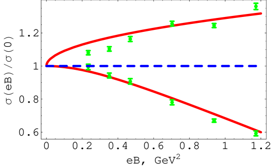
Figure 1: $\sigma(eB)/\sigma(B=0)$ for $B_{\bot}$ (upper red curve) and $B_{\|}$ (lower red curve), in comparison with lattice data from [5] (green points)

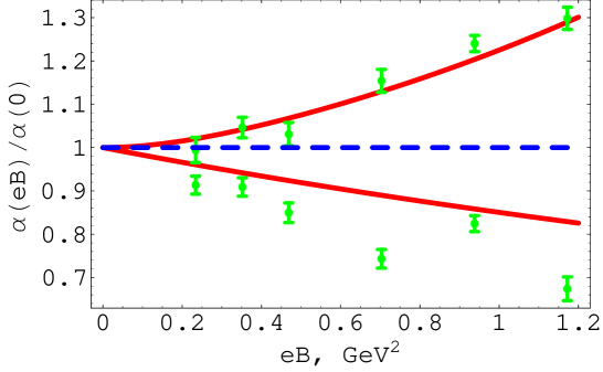
Figure 2: $\alpha_{s}(eB)/\alpha_{s}(B=0)$ for $B_{\bot}$ (lower red curve) and $B_{\|}$ (upper red curve), in comparison with lattice data from [5] (green points)

8 Summary and conclusions

Our discussion above is actually an attempt to qualitatively understand the dynamical mechanism beyond the $\sigma$ and $\alpha_{s}$ dependence on m.f. We have identified two possible effects in the action of external magnetic field on confinement, which can act only through sea quarks loops. The first is the increasing production of loops in m.f. – the focusing effect. The second effect is the energy increase due to loop production, since they become effectively heavier in m.f., and this acts only when m.f. is perpendicular to the area surface. As a result one obtains different signs of combining effects; as shown in Fig. 1 and Fig. 2 and this corresponds to the lattice data [5].

To make quantitative comparison with lattice data of [5, 16, 17] the only fitting parameter is $\rho=\frac{\Delta S}{S}$ which was taken as 0.15 . Note the difficulty in deriving it from the general theory [1, 2, 3], since the corresponding integrals are diverging and need regularization. The results for $\Delta\sigma$ are in a fine agreement with [5].

We have calculated the screening of the $\alpha_{s}(eB)$ due to the quark pair creation in m.f., which occurs in $\mbox{\boldmath${\rm B}$}_{\bot}$ and has the same physical mechanism as in the $q\bar{q}$ energy growth due to m.f., Eq. (10). The stimulated creation of the $q\bar{q}$ pairs in the case of $B_{\|}$ leads to the increase of $\alpha_{s}$. The resulting forms of $\Delta\alpha_{s}$ in Fig. 2 agree with lattice data [5], and we have found the increase of $\alpha_{s}$ in $\mbox{\boldmath${\rm B}$}_{\|}$ due to the enhanced quark loop production, which is an antiscreening effect.

The authors are grateful to Massimo D’Elia for discussions, suggestions and numerical data. The authors are grateful to M.A.Andreichikov, B.O.Kerbikov and members of the ITEP theory seminar for useful discussions. The financial support of the RFBR grant 1402-00395 is gratefully acknowledged.

References

-
[1]
H.G.Dosch, Phys. Lett. B 190, 177 (1987);
H.G.Dosch and Yu.A.Simonov, Phys. Lett. B 205, 339 (1988);
Yu.A.Simonov, Nucl. Phys. B 307, 512 (1988). -
[2]
M.D’Elia, A.Di Giacomo and E.Meggiolaro, Phys. Lett. B 408, 315
(1997); Phys. Rev. D 67 , 114504 (2003):
A.Di Giacomo, H.G.Dosch, V.I.Shevchenko and Yu.A.Simonov, Phys. Rept.372, 319 (2007). -
[3]
Yu.A.Simonov, Phys. Usp. 39, 313 (1996); hep-ph/979344;
Yu.A.Simonov and V.I.Shevchenko, Adv. High. En. Phys. 2009, 873051 (2009); Intern. J. Mod. Phys. A 18, 127 (2003); Phys. Rev. Lett. 85, 1811 (2000). - [4] M.A.Andreichikov, V.D.Orlovsky and Yu.A.Simonov, Phys. Rev. Lett. 110, 162002 (2013).
- [5] C. Bonati, M.D’Elia, M.Mariti and F.Negro, Phys. Rev. D 89 , 114502 (2014).
- [6] Yu. A. Simonov, Phys. Rev. D 88, 025028 (2013).
- [7] Yu. A. Simonov, Phys. Rev. D 88, 053004 (2013).
- [8] M.A.Andreichikov, B.O.Kerbikov, V.D.Orlovsky and Yu.A.Simonov, Phys.Rev. D 87, 094029 (2013).
-
[9]
Yu. A. Simonov, Phys. Rev. D 88, 093001 (2013);
M.A.Andreichikov, B.O.Kerbikov and Yu.A.Simonov JETP Lett, 99, 246 (2014). - [10] A.M.Badalian and Yu.A.Simonov, Phys. Rev. D 87, 074012 (2013).
- [11] Yu. A. Simonov, Phys. Rev. D 84, 065013 (2011).
- [12] A. M. Badalian V.D.Orlovsky and Yu.A.Simonov, Phys. At. Nucl. 76, 955 (2013).
-
[13]
L.Del Debbio, A.Di Giacomo and Yu.A.Simonov, Phys. Lett. B 332
111 (1994);
P.Bicudo, N.Cardoso and M.Cardoso, Phys. Lett. B 710, 343 (2012). - [14] V.I.Shevchenko and Yu.A.Simonov, Phys. Rev. D 66, 056012 (2008).
- [15] D.S.Kuzmenko, Yu.A.Simonov and V.I.Shevchenko, Phys. Usp. 41, 1 (2004).
- [16] G.S.Bali, F.Bruckmann, G.Endrödi and A.Schäfer, Phys. Rev. Lett. 112, 042301 (2014); arXiv: 1311.2559 [hep-lat].
- [17] G.S.Bali, F.Bruckmann, G.Endrödi and A.Schäfer, F.Gruber, JHEP, 1304 , 1303 (2013); arXiv: 1303.1328 [hep-lat].
- [18] M.A.Andreichikov, B.O.Kerbikov, V.D.Orlovsky and Yu.A.Simonov, Phys. Rev. Lett. 110, 162002 (2013); arxiv: 1211.6568.
- [19] M.A.Andreichikov, B.O.Kerbikov, V.D.Orlovsky and Yu.A.Simonov, Phys. Rev. D 87, 094029 (2013); arxiv: 1211.6568.
-
[20]
Yu. M.Loskutov and V.V.Skobelev, Vestnik MGU, physics, astronomy,
24, 95 (1983);
A.V.Kuznetsov, N.V.Mikheev and M.V.Osipov, Mod. Phys. Lett. A 17, 231 (2002). -
[21]
A.E.Shabad and V.V.Usov, Phys. Rev. Lett. 98 180403 (2007);
Phys. Rev. D 77, 125001
(2008):
M.I.Vysotsky, Pis’ma v Zh. Eksp. Teor. Fiz. 92, 22 (2010); B.Machet and M.I.Vysotsky, Phys. Rev. D 83, 025022 (2011). - [22] V.Novikov, M.A.Shifman, A.Vainshtein and V.I.Zakharov, Fortsch. Phys. 32, 585 (1984).
- [23] E.-M.Ilgenfritz, M.Kalinowski, M.Müller-Preussker, B.Petersson and A.Schreiber, Phys. Rev. D 85, 114504 (2012), arXiV: 1303.3972[hep-lat].