Investigating the Impact of Metric Aggregation Techniques on Defect Prediction

Abstract

Code metrics collected at the method level are often aggregated using summation to capture system properties at higher levels (e.g., file- or package-level). Since defect data is often available at these higher levels, this aggregation allows researchers to build defect prediction models. Recent findings by Landman et al. indicate that aggregation is likely to inflate the correlation between size and complexity metrics. In this paper, we explore the effect of nine aggregation techniques on the correlation between three types of code metrics, namely Lines of Code, McCabe, and Halstead metrics. In addition to summation, we study aggregation techniques that are measures of: (1) central tendency (average and median), (2) dispersion (standard deviation and inter-quartile range), (3) shape (skewness and kurtosis), and (4) income inequality (Theil index and Gini coefficient). Our results show that defect prediction models built using summation outperform those built using other aggregation techniques. We also find that more complex aggregations are no different than much simpler ones and that incorporating all aggregation types in the same model does not provide a significant improvement over using summation alone.

1 Introduction

Code metrics can be computed at different levels of granularity to help analyze the defect-proneness of software components. While metrics such as the Chidamber and Kemerer suite (Chidamber and Kemerer, 1994) are defined at the class-level, others such as Lines Of Code (LOC), (McCabe, 1976), and (Halstead, 1977) measure complexity at the module level. These module-level metrics are typically aggregated using sum or average to lift their values to higher levels (Gill and Kemerer, 1991; Lanza and Marinescu, 2006; Mordal-Manet et al, 2011).

Recent findings of Landman et al (2014) suggest that aggregation is likely to amplify the correlation between LOC and other code metrics at the file level, which is consistent with previous results (Li and Cheung, 1987; Jay et al, 2009; Basili and Perricone, 1984; Feuer and Fowlkes, 1979; Curtis et al, 1979a). Their study, which involved a large corpus of Java methods, indicates that the linear correlation between LOC and McCabe’s cyclomatic complexity increases when both metrics are summed over larger units of code. However, it is not known whether this observation generalizes to other types of metrics or other aggregation techniques.

We, therefore, aim to study the impact that different aggregation techniques have on defect prediction at the file level using three types of code metrics, namely LOC, McCabe, and Halstead metrics. In addition to summation, we study aggregation techniques that measure: (1) central tendency (Average and Median), (2) dispersion (Standard Deviation and Inter-quartile Range), (3) shape (Skewness and Kurtosis), and (4) income inequality (Theil index and Gini coefficient). We analyze the aggregated metrics by performing correlation analysis and building regression models with repeated cross-validation. Our empirical study involves 12 releases of three open-source projects and addresses the following research questions:

1. What are the aggregation techniques that do not inflate the correlation between LOC and other metrics at the file level?
   As reported by Landman et al (2014), we find that aggregating the studied complexity metrics using Sum tends to inflate their correlation with LOC at the file level. On the other hand, the correlation with LOC tends to decrease when aggregation is performed using Median as well as the measures of shape and income inequality.

2. Do different aggregation techniques convey different information?
   Yes, although we observe high rates of correlation among aggregations of the same family (e.g., Skewness and Kurtosis, Theil and Gini), the redundancy among aggregations of different families remains low.

3. Does the type of aggregation used in defect prediction models matter?
   Using repeated 10-fold cross validation, our results show that defect prediction models built using summation outperform those built using other aggregation techniques. We also conclude that incorporating all aggregation types in the same model does not provide a significant improvement over using summation alone.

The remainder of the paper is organized as follows. Section 2 discusses related work within the context of metric aggregation. Section 3 describes our experimental setup by elaborating on the code metrics and aggregation techniques that we use. It also presents our regression models along with the evaluation criteria. Section 4 presents a detailed analysis of the results. Section 5 discusses the threats to the validity of our findings. Finally, Section 6 concludes our work and points out possible future enhancements.

2 Related Work

There seems to be a trade-off between the simplicity of an aggregation method and its suitability to represent the data accurately. While the former is important to arrive at an easy-to-describe aggregation, the latter is necessary to provide reliable decisions about software maintainability. For example, even though Sum is a simple metric, it was recently shown to render some code metrics redundant (Landman et al, 2014). Also, simple measures of central tendency such as the mean are often deemed inappropriate when the underlying data is skewed (Concas et al, 2007; Vasa et al, 2009). As a result, several aggregation approaches were proposed in literature to overcome such limitations.

One family of metric aggregation techniques uses income inequality measures that were originally proposed to quantify the imbalance in wealth distribution in a given population. In this regard, Vasa et al (2009) use the Gini coefficient (Gini, 1912) on class-level metrics to understand the evolution of object-oriented systems. Their results indicate that the Gini coefficients do not change significantly between adjacent releases and that the relatively high values of such coefficients indicate that developers tend to prefer centralized and complex abstractions over distributed and simple ones. On the other hand, Serebrenik and van den Brand (2010) propose using Theil index (Theil, 1967) instead of the Gini coefficient for metric aggregation as the latter is not decomposable among separate groups of a given population. They argue that decomposability highlights intra-group and inter-group inequality and thus is essential to explain the inequality among a given population rather than just measuring it.

Another approach for metric aggregation relies on fitting a statistical distribution to the set of observed metric values. In this sense, the aggregation would be based on the estimated values of the distribution parameters. It is evident that the viability of such approach is dependent on the choice of statistical distribution as well as the dataset being used. For example, while Tamai and Nakatani (2002) report that size data such as the number of methods per class and the number of lines of code per method follow a negative binomial distribution, Concas et al (2007) argue that the former follows a log-normal distribution and the latter follows a power-law.

3 Experimental Design

Our study involves 12 releases of three open source projects: Eclipse, Apache Ant, and jEdit. Eclipse (eclipse.org) is a cross-platform IDE with an extensible plug-in architecture. Ant (ant.apache.org) is a build tool implemented in Java - initially proposed as an alternative to Unix make. jEdit (jedit.org) is a Java-based text editor targeted for programmers. Table 1 shows, for each project, the releases that we used as well as the download locations where we obtained the corresponding source code and post-release defect information.

Table 1: Studied Projects.

	Releases	Source code	Post-release defects
Eclipse	2.0, 2.1, 3.0	archive.eclipse.org	st.cs.uni-saarland.de
Ant	1.3, 1.4, 1.5, 1.6, 1.7	archive.apache.org	code.google.com/p/promisedata
jEdit	4.0, 4.1, 4.2, 4.3	sourceforge.net	code.google.com/p/promisedata

After obtaining the source code of the 12 releases, we used McCabe IQ 8.3 (McCabe Software, 2014) to collect three types of method-level code metrics: LOC, McCabe, and Halstead metrics. These metrics are then aggregated to the file level via nine aggregation techniques. Using the aggregated metrics and the post-release defect information, we build regression models to study the impact of the different aggregations on defect prediction. Figure 1 shows an overview of our approach.

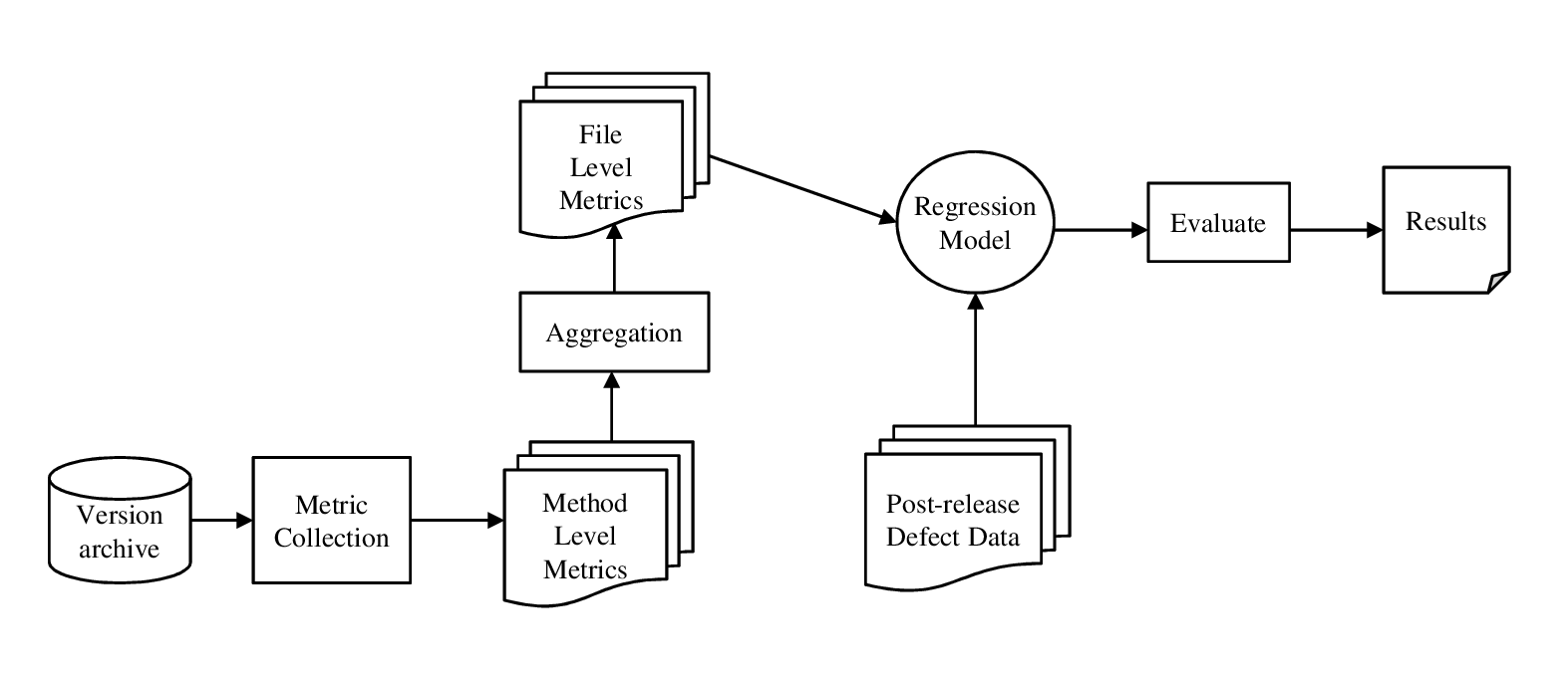
Figure 1: Approach overview.

3.1 Code Metrics

Code metrics are relatively easy to compute and are widely used in literature (Sunohara et al, 1981; Menzies et al, 2004; Zhang, 2009; Zimmermann et al, 2007; Jiang et al, 2008; Curtis et al, 1979b; Menzies et al, 2007; Khoshgoftaar and Munson, 1990) to assess software quality, build prediction models, understand maintenance complexity, etc. In this work, we consider three types of commonly used code metrics: LOC, McCabe, and Halstead metrics. While McCabe metrics such as cyclomatic complexity (McCabe, 1976) aim at measuring the complexity associated with a software module using the number of forks in the corresponding control-flow graph, Halstead metrics estimate the complexity using the number of operators and operands in the module. Table 2 lists the metrics we use in our study and provides a brief description of each as described in McCabe Software (2014).

Table 2: Code metrics used.

Metric	Type	Description
LOC	-	Total number of lines in a module
Cyclomatic Complexity (v(G))	McCabe	Number of linearly independent paths in the flow-graph of a module
Essential Complexity (ev(G))	McCabe	Degree to which a module contains unstructured constructs
Module Design Complexity (iv(G))	McCabe	Complexity of the design reduced module
Program Volume (V)	Halstead	Minimum number of bits required for coding the program
Program Difficulty (D)	Halstead	Level of difficulty in the program
Program Length (N)	Halstead	Total number of operators and operands
Program Level (L)	Halstead	Level at which the program can be understood
Intelligent Content (I)	Halstead	Complexity of a given algorithm independent of the language used
Programming Effort (E)	Halstead	Estimated mental effort required to develop the program
Error Estimate (B)	Halstead	Estimated number of errors in the program
Programming time (T)	Halstead	Estimated amount of time to implement the algorithm

3.2 Aggregation Techniques

For a given module $D$ and a code metric $M$, we denote by $M(D)$ the value of $M$ when applied to $D$. For example $LOC(foo)$ is the number of lines of code in method $foo$. If a file $F$ contains $N$ methods ${D_{1},D_{2},...,D_{N}}$, then $M$ could be defined for $F$ by aggregating the values $M(D_{1}),M(D_{2}),...,M(D_{N})$. Such aggregation could be done in different ways, giving rise to different interpretations of $M$ at the file level. For example, aggregating $LOC$ by Sum would result in a file-level metric (say Sum(LOC)) that measures the overall size of $F$. However, aggregating it using Standard Deviation would result in a different file-level metric (SD(LOC)). In this work, we consider nine aggregation techniques including the typical Sum. For a given set of values $X=\{x_{1},x_{2},...,x_{N}\}$ we define the nine aggregation techniques as follows. Note that $Q_{1}(X)$, $Q_{2}(X)$, and $Q_{3}(X)$ denote the first, second, and third quartiles of X respectively.

3.2.1 Summation

$Sum(X)=\sum\limits_{i=1}^{N}x_{i}$

3.2.2 Measures of Central Tendency

• Average: $Avg(X)=\bar{X}=\frac{Sum(X)}{N}$

• Median: $Med(X)=Q_{2}(X)$

3.2.3 Measures of Dispersion

• Standard deviation: $SD(X)=\sqrt{\frac{\sum\limits_{i=1}^{N}(x_{i}-\bar{X})^{2}}{N-1}}$
  

• Inter-quartile range: $IQR(X)=Q_{3}(X)-Q_{1}(X)$

3.2.4 Measures of Shape

• Skewness: $Skew(X)=\frac{\frac{\sum\limits_{i=1}^{N}(x_{i}-\bar{X})^{3}}{N}}{(\frac{\sum\limits_{i=1}^{N}(x_{i}-\bar{X})^{2}}{N-1})^{\frac{3}{2}}}$
  

• Kurtosis: $Kurt(X)=\frac{\frac{\sum\limits_{i=1}^{N}(x_{i}-\bar{X})^{4}}{N}}{(SD(X))^{4}}-3$

3.2.5 Income Inequality Measures

• Theil index: $Theil(X)=\frac{1}{N}\sum\limits_{i=1}^{N}(\frac{x_{i}}{\bar{X}}ln\frac{x_{i}}{\bar{X}})$
  

• Gini coefficient: $Gini(X)=\frac{2\sum\limits_{i=1}^{N}ix^{\prime}_{i}}{N\sum\limits_{i=1}^{N}x^{\prime}_{i}}-\frac{N+1}{N}$
  where $\{x^{\prime}_{1},x^{\prime}_{2},...,x^{\prime}_{N}\}$ is a sorted version of $X$.

3.3 Selection of Predictors

Given that we have 12 metrics and 9 aggregation techniques, it follows that there are 108 predictors to account for in our regression models. However, prior to building the models, it is important to mitigate any potential redundancy among these predictors to avoid model instability and degradation in predictive performance (Kuhn and Johnson, 2013). Redundancy among predictors exists in two forms: pairwise correlation and multi-collinearity. While correlation measures the degree of association between pairs of variables, multi-collinearity refers to the situation when there is a concurrent relationship between multiple variables, i.e. when some variables could be predicted from a combination of other ones. In this work, we pre-process the set of predictor variables by applying correlation and multi-collinearity analyses as follows:

1. Correlation analysis: We use Varclus (Sarle, 1990) to analyze correlations among the predictor variables. Varclus is a hierarchical approach that depicts variables in clusters each of which is associated with a correlation level. We consider Spearman rank correlation ($\rho$) such that, for each cluster with $|\rho|>0.7$, we select one variable and discard all the rest. We use the varclus function provided by the Hmisc package in R (R Core Team, 2014) to perform this analysis.

2. Multi-collinearity analysis: The variables retained from the previous step are further analyzed to check for potential multi-collinearity. We perform such analysis by considering how well each variable is predicted by the others. Variables that are highly predictable are discarded in an iterative fashion until all remaining variables exhibit low levels of redundancy. Specifically, we quantify the predictability of a particular variable v by fitting a linear regression model that uses v as response and the other variables as predictors. We then use the adjusted coefficient of determination $R^{2}$, which represents the goodness of fit, to measure the predictability of v. Therefore, in each iteration, we compute the $R^{2}$ for all variables and drop the one associated with the highest value. This process is repeated until all the $R^{2}$ values are below a cutoff threshold. This approach is implemented via function redun provided by the Hmisc package in R, which uses a default cutoff threshold of 0.9.

We refer to the pre-processing stage comprising these two steps as the ”filtering” phase since it is used to filter the predictor variables that are used in the models. Since this phase could be applied on the method-level metrics as well as the aggregated ones, we propose two alternatives for selecting the predictor variables, which we describe next.

3.3.1 One-level filtering approach

In this approach, we first perform aggregation to obtain the file-level metrics. Then, we apply the filtering mechanism on the resulting 108 variables. Figure 2 shows an overview of this approach where the method-level metrics are denoted by $M_{1}$, $M_{2}$, …, $M_{N}$ and the aggregation functions by $A_{1}$, $A_{2}$, …, $A_{P}$.

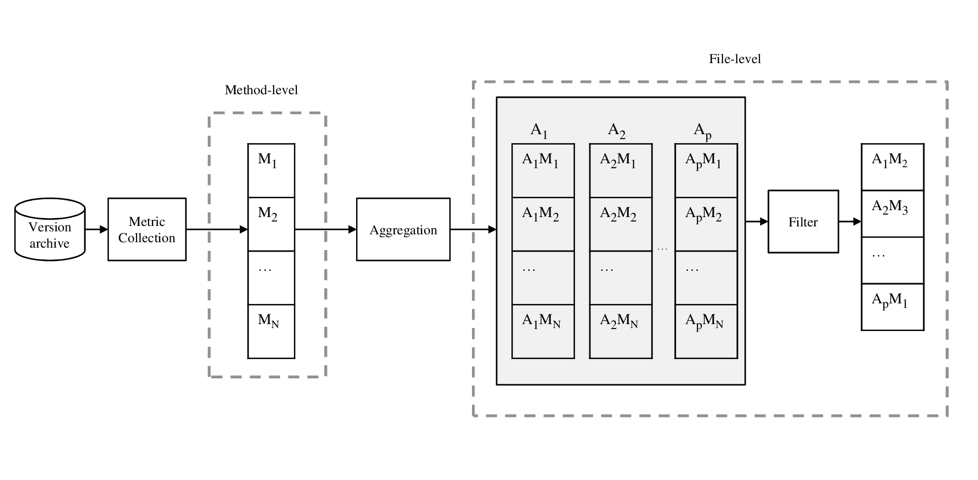
Figure 2: One-level filtering approach (the final set of variables is depicted randomly).

3.3.2 Two-level filtering approach

This approach is depicted in Figure 3. In contrast to the previous approach, we first apply filtering on the method-level metrics to obtain $M_{i}$, $M_{j}$, …, $M_{k}$. These metrics are then aggregated to the file level using each of the aggregation techniques. At the file level, we re-apply filtering to obtain the final set of predictor variables.

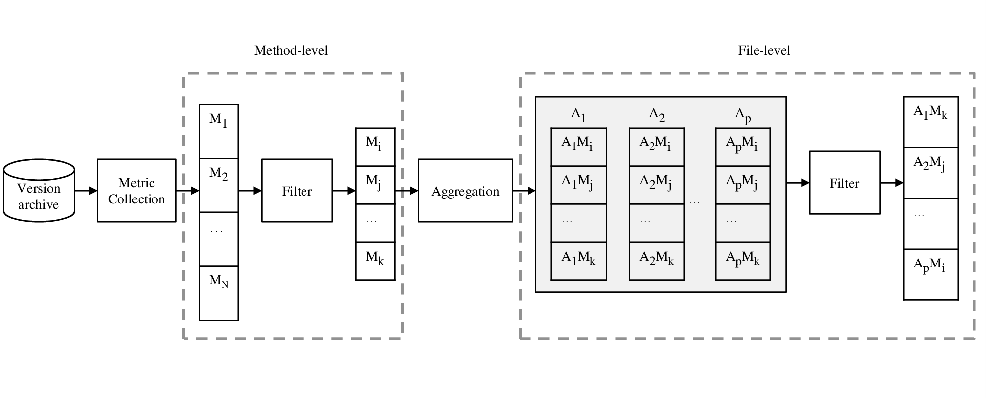
Figure 3: Two-level filtering approach (the final set of variables is depicted randomly).

3.4 Defect Prediction using Aggregated Code Metrics

Defect prediction aims at modeling the relationship between a set of explanatory (i.e. predictor) variables and the fault-proneness of a software component (dependent variable). In this work, we use as predictor variables the set of aggregated metrics resulting from the two aforementioned filtering approaches. We study the impact of such metrics on the accuracy of defect prediction by building linear and logistic regression models having the file-level defect information as the dependent variable.

3.4.1 Regression Models

Linear regression uses a linear equation of the form $\beta_{0}+\beta_{1}x_{1}+...+\beta_{n}x_{n}$ to predict the value of the dependent variable, where $x_{1},...,x_{n}$ are assumed to be the predictor variables. The regression coefficients $\beta_{0},\beta_{1},...,\beta_{n}$ are usually determined relative to a given training set using Least-squares estimation. In our case, we use linear regression to predict the number of post-release defects that are likely to be present in a given file.

As opposed to linear regression, the dependent variable in logistic regression is a binary variable, indicating whether a file has defects or not. This outcome is predicted using a logistic function of the form $\frac{1}{1+e^{-(\beta_{0}+\beta_{1}x_{1}+...+\beta_{n}x_{n})}}$. The output would be a value between 0 and 1. Typically, a file would be classified as defective if the output is greater than $0.5$.

In our analysis, we use the implementations lm and glm provided by R (R Core Team, 2014) to build the linear and logistic models respectively.

3.4.2 Performance Measures

We evaluate the predictive accuracy of our regression models using repeated 10-fold cross validation (Witten and Frank, 2005). Specifically, we partition each dataset $D$ into 10 equally-sized disjoint subsets $S_{1},S_{2},...,S_{10}$. For each subset $S_{i}$, we use $D-S_{i}$ to build the model and $S_{i}$ for prediction. The whole process is then repeated 10 times to account for the effect of randomness.

In each iteration, we measure the accuracy of the linear models by computing the mean squared error (MSE) between the predicted values and the actual ones. As for the logistic models, we use the area under the ROC curve (Bradley, 1997) (AUC) which is commonly used to evaluate binary classifiers. AUC ranges between 0 and 1 where higher values indicate better performance. As such, a random classifier would have an AUC of 0.5. We report the average values for MSE and AUC metrics across all the iterations of the cross-validation.

4 Results

In this section, we present the results of our empirical study with respect to our three research questions.

(RQ1) What are the aggregation techniques that do not inflate the correlation between LOC and other metrics at the file level?

In an ideal situation, one would desire aggregation techniques that preserve as much information as possible about the signals exhibited by method-level metrics when lifting their values to the file level. However, previous research indicates that aggregating certain metrics to the file level using summation inflates their correlation with LOC (Landman et al, 2014; Li and Cheung, 1987; Jay et al, 2009; Basili and Perricone, 1984; Feuer and Fowlkes, 1979; Curtis et al, 1979a). This might have a detrimental effect as many metrics might become redundant at the file level. This research question aims at investigating how aggregation techniques other than the typical summation affect the correlation with LOC at the file level. We address this issue by comparing correlations before and after aggregation. Specifically, we first compute the Spearman rank correlation $\rho$ between $LOC$ and every other metric at the method level. Then, for each aggregation technique $A$ and each metric $M$, we compute $\rho$ for $A(LOC)$ and $A(M)$. In our analysis, we consider the absolute value of $\rho$ since we are interested in the degree of correlation rather than its polarity. Table 3 reports the average increase in $|\rho|$ across all 12 datasets between $LOC$ and each code metric, according to the nine aggregation functions. For example, the average increase in $|\rho|$ for LOC and cyclomatic complexity when Sum is used for aggregation is 14%.

Table 3: Average increase in Spearman rank correlation with LOC at the file level.

	Sum	Avg	Med	SD	IQR	Skew	Kurt	Theil	Gini
v(G)	14%	4%	-5%	4%	3%	1%	0%	0%	2%
ev(G)	83%	27%	-28%	38%	4%	27%	35%	26%	26%
iv(G)	16%	5%	-7%	6%	2%	1%	-1%	1%	3%
N	6%	4%	0%	4%	3%	0%	-1%	-5%	-5%
V	5%	4%	0%	4%	3%	0%	-1%	-11%	-12%
L	-10%	-24%	-5%	-77%	-87%	-51%	-8%	-31%	-24%
D	8%	-1%	-3%	-5%	-5%	-7%	-3%	-25%	-21%
I	9%	-3%	-1%	-4%	-4%	-8%	-2%	-22%	-18%
E	1%	1%	0%	2%	2%	-1%	-2%	-18%	-19%
B	5%	4%	0%	4%	3%	-1%	-1%	-23%	-20%
T	1%	1%	0%	2%	2%	-1%	-2%	-18%	-19%

The results clearly show that the increase in correlation depends on the metric being considered as well as the aggregation function used. For all metrics, except Halstead’s program level (L), there is at least one aggregation function that increases its correlation with LOC and another one that decreases it. Moreover, it can be noticed that most aggregation functions other than Sum generally tend to decrease the correlation rather than increase it, especially for the Halstead metrics.

Our conclusions regarding Sum are in line with previous research in the sense that it tends to increase correlation at the file level. However, we find this increase rather moderate as it ranges between $1\%$ and $16\%$ for all metrics except McCabe’s essential complexity (ev(G)) and Halstead’s program level (L). Also, for most of the metrics, Sum results in the highest increase among all the aggregation functions.

Concerning Avg, SD, and IQR, we notice a similar pattern to that associated with Sum although they generally result in lower increase rates. In contrast to Sum, all of them decrease the correlation for Halstead’s program difficulty (D) and intelligent content (I).

On the other hand, the results indicate that the overall tendency among Med, measures of shape (Skew and Kurt), and income inequality measures (Theil and Gini) is to decrease the correlation with LOC at the file level rather than increasing it. One might argue that this would be as misleading as increasing the correlation. However, we believe it is not harmful as long as it does not render file-level metrics redundant while their method-level counterparts are not. In this regard, we notice that Med is the only aggregation that does not inflate the correlation for any metric and, even for the cases where it decreases the correlation, we find that the decrease is generally low. With the exception of essential complexity ev(G), we can draw similar conclusions regarding the measures of shape. Concerning the income inequality measures, the overall decrease associated with them is more significant as it ranges between $5\%$ and $31\%$ for Theil and between $5\%$ and $24\%$ for Gini.

Sum increases file-level correlation between most of the studied metrics and LOC. Conversely, Median as well as the measures of shape and income inequality tend to decrease such correlation.

(RQ2) Do different aggregation techniques convey different information?

In the previous research question, we investigated the redundancy of different file-level aggregated code metrics with respect to LOC. Nevertheless, it is also important to study different forms of redundancy among the aggregation techniques themselves; i.e., to check whether aggregating the same metric using different techniques would yield different signals. If this is the case, then one would expect to build defect prediction models with better explanatory power by incorporating all such aggregations if possible. We address this research question by assigning to each aggregated metric a ”redundancy measure” that ranges between 0 and 1 where higher values indicate higher redundancy. We compute such redundancy measure using correlation and multi-collinearity analysis in a similar way to that presented in Section 3.3. For each code metric $M$, we quantify the redundancy associated with each aggregation function $A_{i}$ as follows:

1. Correlation analysis: We apply Varclus on the set ${A_{1}(M),A_{2}(M),...,A_{9}(M)}$ and choose only one metric from each cluster having $|\rho|>0.7$. The metric to be chosen is the one that has the lowest rank in the following order: Sum, Avg, Med, SD, IQR, Skew, Kurt, Theil, and Gini. For example, if the cluster contains Theil(M), Med(M), and IQR(M), we choose Med(M) to be retained and discard all the rest. The order we devise is based on our judgment regarding the complexity associated with each aggregation. For example, we believe that measures of central tendency are simpler than measures of dispersion which are simpler than the measures of shape. We also consider Sum to be the simplest aggregation and the measures of income inequality to be the most complex. The metrics discarded in this stage are assigned a redundancy measure of 1 and the remaining ones will be evaluated in the next step.

2. Multi-collinearity analysis: Using the aggregations obtained from the previous step, we build a linear regression model with $A_{i}(M)$ as the dependent variable and the remaining aggregations as predictors. We then quantify the redundancy associated with $A_{i}(M)$ using the adjusted coefficient of determination $R^{2}$. Therefore, a high value of $R^{2}$ would mean that aggregating $M$ using $A_{i}$ conveys a redundant signal as it can be well-predicted by the remaining aggregations. In this paper, we use a cutoff threshold of 0.9 to determine whether a signal is redundant or not.

We conduct the analysis per code metric for all aggregations. That is, for each metric, we compute the redundancy measure for all of its possible aggregations. The results we obtained are shown as box plots for three metrics: LOC in Figure 4, McCabe’s cyclomatic complexity in Figure 5, and Halstead’s program level in Figure 6. For the remaining metrics we just present the median values in Table 4.

Figure 4 shows that aggregating LOC using Sum or Skew results in unique signals as the redundancy measures for these aggregations are relatively low. For Sum, the redundancy measures range between 0.27 and 0.58 with a median of 0.36 and for Skew they range between 0.32 and 0.6 with a median of 0.49. On the other hand, it can be noticed that the redundancy measures associated with Kurt and Gini are equal to 1 in all 12 datasets. This is due to the fact that these aggregations were discarded in the correlation analysis phase. Specifically, we found that Kurt is generally correlated with Skew and Gini is usually correlated with Theil. Concerning the other aggregations, they do exhibit significantly higher redundancy measures than Sum and Skew but not to the extent to be considered completely redundant. In fact, each of them is deemed non-redundant (i.e. redundancy measure $<0.9$) in at least 3 out of the 12 datasets we analyzed.

We make the same general conclusions with respect to the different aggregations of cyclomatic complexity, shown in Figure 5. The results, however, show that both of the income inequality measures are entirely redundant and that Kurt exhibits some uniqueness in its signal. Concerning Halstead’s program level (L), Figure 6 shows that Sum is associated with the lowest redundancy values which range between $0.12$ and $0.23$. We also find that the measures of shape, and to a lesser extent, Avg and SD exhibit satisfactory uniqueness in their signals. On the other hand, Med, IQR, and Gini are entirely redundant.

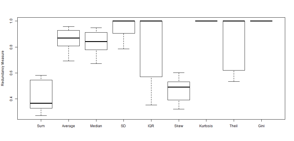
Figure 4: The distribution of the redundancy measures for each aggregation of LOC across the 12 datasets.

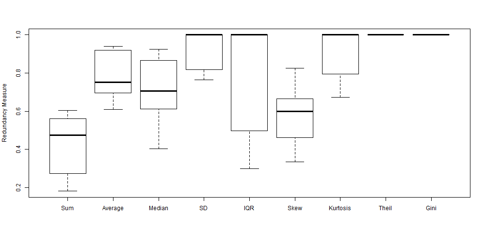
Figure 5: The distribution of the redundancy measures for each aggregation of McCabe’s cyclomatic complexity v(G) across the 12 datasets.

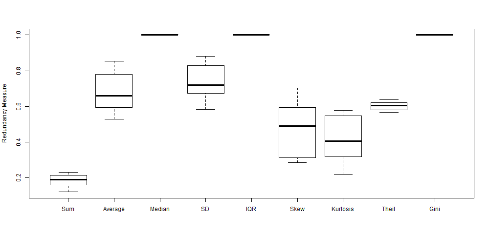
Figure 6: The distribution of the redundancy measures for each aggregation of Halstead’s program level (L) across the 12 datasets.

Table 4: The median value of redundancy measures per code metric across the 12 datasets.

	Sum	Avg	Med	SD	IQR	Skew	Kurt	Theil	Gini
ev(G)	0.45	0.78	0.53	1.00	0.62	1.00	0.32	1.00	1.00
iv(G)	0.46	0.67	0.64	1.00	1.00	1.00	0.35	1.00	1.00
V	0.49	0.82	0.81	1.00	1.00	0.62	1.00	0.58	1.00
D	0.32	0.72	1.00	0.80	1.00	0.36	1.00	0.53	1.00
N	0.45	0.86	0.85	1.00	1.00	0.57	1.00	0.61	1.00
I	0.32	0.67	1.00	0.76	1.00	0.40	1.00	0.55	1.00
E	0.20	1.00	0.07	1.00	1.00	0.68	1.00	0.58	1.00
B	0.34	1.00	0.15	1.00	1.00	0.56	1.00	0.42	1.00
T	0.20	1.00	0.07	1.00	1.00	0.68	1.00	0.58	1.00

Table 4 shows, for each of the remaining code metrics, the median value of the redundancy measures associated with each of its aggregations across the 12 datasets. For example, the median redundancy measure of $Sum(ev(G))$ is 0.45. It can be noticed that Sum is the only aggregation that results in a non-redundant signal for all code metrics. The corresponding redundancy measure ranges between 0.2 and 0.49. In fact, all other aggregations except Gini result in a relatively non-redundant signal for at least one code metric. Examples include Avg(iv(G)), Med(E), SD(I), IQR(ev(G)), Skew(D), Kurt(ev(G)), and Theil(B). Nevertheless, it is evident that the measures of dispersion, kurtosis and Theil index tend to result in signals with higher redundancy levels.

The main conclusion we draw regarding this research question is that different aggregations do convey different signals about the underlying metrics - even though some exhibit this pattern more frequently than the others. This means that code metrics could be represented at the file level by several non-redundant signals - which would be more informative than using one type of aggregation only.

Each of the studied aggregations, except Gini, provides a non-redundant signal for at least one code metric. Sum exhibits non-redundancy for all metrics.

(RQ3) Does the type of aggregation used in defect prediction models matter?

The results of the two previous research questions indicate that it is possible to retain file-level aggregated metrics that are not redundant with respect to one another. Specifically, in RQ1 we found that certain aggregations do not inflate the correlation with LOC and in RQ2 we found that most studied aggregations exhibit non-redundant signals for at least one code metric. As such, we aim at investigating whether these findings could be leveraged to improve file-level defect prediction. We do so by evaluating the accuracy of defect prediction models built using each type of aggregation separately. That is, for each aggregation $A$, we build linear and logistic regression models that predict the incidence of post-release defects using the 12 code metrics aggregated to the file level using $A$. In addition, we investigate a ”full” model that incorporates all the aggregations of all the code metrics at once. We denote this model by All and use it as a means to check whether the different signals conveyed by different aggregations have an additive effect on the accuracy of defect prediction. If this is the case, then such model would outperform all models that involve one type of aggregation only. We perform predictor selection using the two approaches presented in section 3.3 and use repeated 10-fold cross validation to test our models. We measure the accuracy of the linear models using the mean-squared error of prediction and evaluate the performance of the logistic models using AUC. Table 6 shows the average MSE that we obtained for the linear models across all the iterations of the repeated cross validation. Similarly, Table 7 shows the average AUC for the logistic models. Rows denoted by F1 (resp. F2) correspond to the models built using the One-level (rep. Two-level) filtering approach.

Table 6 shows that, among the nine aggregation techniques, the linear models built using Sum outperform those built with other aggregations for most of the datasets as they achieve lower values of MSE. We also find that aggregations pertaining to the same family yield similar results and that the measures of shape outperform the measures of dispersion and income inequality.

The results do not support the expectation that the full model would outperform those built using one type of aggregation only. When comparing the full model to the one built using Sum, we notice a marginal improvement for the Eclipse 2.0, Eclipse 3.0, and Ant 1.7 datasets. For the remaining datasets, Sum results in MSE values that are less than or equal to those achieved by All. With respect to the other aggregations, the full model achieves slightly better results for all datasets except Ant 1.3, Ant 1.4, and Ant 1.5.

Another observation that could be deduced from the results is that One-level and Two-level filtering mechanisms result in similar MSE values. This means that the filtering approach does not have a significant influence on the prediction accuracy. As such, it would be obvious to favor the one that retains fewer predictor variables as it would result in a more comprehensible model that is simple to communicate. Table 5 shows the average number of variables retained by each filtering approach across the 12 datasets. The numbers adjacent to the aggregation type represent the total number of independent variables to account for. While both approaches result in major reductions, our findings indicate that Two-level filtering consistently results in fewer predictor variables and, thus, would be more suitable for model analysis.

Table 5: Average number of variables retained by the two filtering approaches.

	One-level Filtering	Two-level Filtering
All (108)	18.6	13.8
Sum (12)	2.0	2.0
Avg (12)	3.6	2.7
Med (12)	3.7	3.0
SD (12)	3.7	2.6
IQR (12)	3.6	3.0
Skew (12)	3.7	2.7
Kurt (12)	3.2	2.5
Theil (12)	4.7	2.7
Gini (12)	4.7	3.0

Similarly to the linear regression results, we find that the logistic models built with Sum generally outperform those built using other aggregations. With the exception of the Ant 1.4 dataset, Sum achieves higher AUC values for all studied projects. Sum also outperforms the full model for releases 1.5, 1.6, and 1.7 of Ant, as well as releases 4.1 and 4.2 of jEdit. The differences however are not significant as they range between 0.02 and 0.04. On the other hand, the full model achieves marginally better results with respect to the three releases of Eclipse in addition to releases 4.0 and 4.3 of jEdit.

In summary, Tables 6 and 7 show that incorporating all aggregations in the same model does not enhance the accuracy of linear or logistic defect prediction models. Specifically, we could not observe a general improvement induced by the full model (All) with respect to the Sum model that resulted in the best performance among the studied aggregations. This comparison was done according to the average MSE and AUC values across all the iterations of the cross validation. To further analyze the statistical significance of any potential differences between the All and Sum models, we use the Mann-Whitney U test. In addition to checking whether the MSE (and AUC) values exhibited by both models are statistically significant, we also quantify the extent of this difference (effect size) using Cliff’s $|d|$ (Macbeth et al, 2011). In this regard, Romano et al (2006) provide three thresholds to interpret the values of $|d|$: 0.147, 0.33, and 0.474. The effect would be considered negligible if it is less than 0.147, small if it is between 0.147 and 0.33, medium if it is between 0.33 and 0.474, and large otherwise. Table 8 shows, for each dataset, the statistical significance of the Mann-Whitney U test (p-value) in addition to Cliff’s $|d|$. Concerning the results of the linear regression, we find that the difference between the two sets of MSE values is statistically significant for all datasets. However, the effect size is negligible for most of them and small with respect to Ant 1.5 and jEdit 4.3. On the other hand, the difference between the sets of AUC values exhibited by the regression models is statistically significant for half of the datasets. Among these datasets, the effect size is negligible for Eclipse 3.0 and small for the rest. These findings support our conclusion that different aggregations do not have an additive effect on the accuracy of file-level defect prediction.

The studied aggregations do not have an additive effect on the accuracy of defect prediction. Regression models built with all aggregations at once are not better than those built using Sum only.

Table 6: Average MSE achieved by the linear models across the different iterations of the cross-validation. F1 (resp. F2) corresponds to the models built using the One-level (rep. Two-level) filtering approach.

		All	Sum	Avg	Med	SD	IQR	Skew	Kurt	Theil	Gini
Eclipse 2.0	F1	0.88	0.90	1.00	1.02	0.98	1.01	0.94	0.94	0.98	0.98
	F2	0.91	0.91	1.00	1.02	0.98	1.01	0.95	0.95	0.98	0.98
Eclipse 2.1	F1	0.30	0.30	0.32	0.32	0.32	0.32	0.31	0.31	0.32	0.32
	F2	0.30	0.30	0.32	0.32	0.32	0.32	0.31	0.31	0.32	0.32
Eclipse 3.0	F1	0.89	0.92	1.01	1.05	1.00	1.04	0.96	0.96	1.01	1.01
	F2	0.92	0.92	1.02	1.05	0.99	1.04	0.96	0.97	1.01	1.01
Ant 1.3	F1	0.56	0.47	0.53	0.51	0.52	0.51	0.51	0.53	0.51	0.52
	F2	0.54	0.47	0.52	0.52	0.51	0.51	0.50	0.53	0.53	0.53
Ant 1.4	F1	0.37	0.32	0.32	0.32	0.32	0.33	0.32	0.33	0.32	0.32
	F2	0.36	0.32	0.32	0.32	0.32	0.33	0.32	0.32	0.31	0.32
Ant 1.5	F1	0.13	0.12	0.14	0.14	0.14	0.14	0.13	0.12	0.13	0.13
	F2	0.13	0.12	0.14	0.14	0.13	0.14	0.12	0.12	0.13	0.13
Ant 1.6	F1	1.13	1.03	1.49	1.52	1.39	1.48	1.18	1.20	1.34	1.37
	F2	1.10	1.03	1.49	1.52	1.39	1.48	1.23	1.25	1.35	1.37
Ant 1.7	F1	1.01	1.04	1.38	1.42	1.23	1.42	1.15	1.19	1.17	1.24
	F2	1.05	1.05	1.38	1.42	1.25	1.42	1.15	1.20	1.19	1.26
jEdit 4.0	F1	4.70	4.61	6.09	6.08	6.05	6.15	5.25	5.54	6.00	5.81
	F2	4.78	4.70	6.09	6.08	6.00	6.14	5.08	5.22	5.95	5.79
jEdit 4.1	F1	3.02	2.86	3.77	3.85	3.74	3.87	3.32	3.70	3.73	3.61
	F2	3.10	2.84	3.77	3.84	3.75	3.87	3.31	3.67	3.73	3.63
jEdit 4.2	F1	1.03	0.96	1.23	1.25	1.22	1.25	1.12	1.06	1.22	1.19
	F2	1.08	0.97	1.23	1.25	1.22	1.24	1.10	1.05	1.21	1.19
jEdit 4.3	F1	0.03	0.03	0.03	0.03	0.03	0.03	0.03	0.03	0.03	0.03
	F2	0.03	0.03	0.03	0.03	0.03	0.03	0.03	0.03	0.03	0.03

Table 7: Average AUC achieved by the logistic models across the different iterations of the cross-validation. F1 (resp. F2) corresponds to the models built using the One-level (rep. Two-level) filtering approach.

		All	Sum	Avg	Med	SD	IQR	Skew	Kurt	Theil	Gini
Eclipse 2.0	F1	0.76	0.75	0.68	0.64	0.71	0.66	0.71	0.66	0.71	0.71
	F2	0.75	0.75	0.69	0.64	0.71	0.66	0.71	0.66	0.70	0.71
Eclipse 2.1	F1	0.71	0.70	0.64	0.60	0.66	0.61	0.68	0.66	0.66	0.67
	F2	0.71	0.70	0.63	0.60	0.65	0.61	0.68	0.66	0.66	0.67
Eclipse 3.0	F1	0.75	0.75	0.65	0.60	0.67	0.63	0.72	0.70	0.66	0.68
	F2	0.74	0.75	0.65	0.60	0.67	0.63	0.71	0.69	0.66	0.68
Ant 1.3	F1	0.73	0.80	0.69	0.73	0.69	0.74	0.72	0.74	0.70	0.72
	F2	0.81	0.80	0.70	0.75	0.68	0.77	0.76	0.77	0.71	0.73
Ant 1.4	F1	0.65	0.64	0.67	0.66	0.64	0.63	0.62	0.64	0.64	0.65
	F2	0.64	0.66	0.67	0.69	0.67	0.64	0.67	0.64	0.69	0.68
Ant 1.5	F1	0.76	0.78	0.67	0.63	0.73	0.66	0.76	0.75	0.74	0.74
	F2	0.76	0.78	0.68	0.62	0.75	0.67	0.76	0.74	0.75	0.74
Ant 1.6	F1	0.80	0.84	0.67	0.58	0.73	0.61	0.80	0.76	0.74	0.75
	F2	0.80	0.84	0.68	0.58	0.73	0.62	0.78	0.75	0.74	0.74
Ant 1.7	F1	0.80	0.81	0.68	0.55	0.73	0.56	0.77	0.76	0.75	0.74
	F2	0.79	0.81	0.68	0.57	0.72	0.56	0.77	0.75	0.74	0.73
jEdit 4.0	F1	0.80	0.78	0.64	0.65	0.65	0.62	0.75	0.72	0.65	0.67
	F2	0.78	0.78	0.65	0.63	0.66	0.61	0.75	0.72	0.65	0.67
jEdit 4.1	F1	0.80	0.83	0.65	0.62	0.68	0.63	0.78	0.77	0.67	0.69
	F2	0.80	0.83	0.66	0.64	0.67	0.63	0.78	0.77	0.68	0.69
jEdit 4.2	F1	0.79	0.84	0.65	0.62	0.66	0.60	0.79	0.75	0.68	0.70
	F2	0.81	0.84	0.66	0.63	0.68	0.60	0.79	0.75	0.70	0.72
jEdit 4.3	F1	0.78	0.75	0.72	0.72	0.76	0.78	0.71	0.70	0.67	0.67
	F2	0.76	0.75	0.66	0.67	0.72	0.68	0.68	0.74	0.69	0.64

Table 8: The results of Mann-Whitney U test and Cliff’s delta concerning the difference in predictive accuracy between All and Sum models.

	Linear		Logistic
	p-value	Cliff’s $|d|$	p-value	Cliff’s $|d|$
Eclipse 2.0	$<0.001$	0.046	$<0.001$	0.157
Eclipse 2.1	$<0.001$	0.008	0.610	0.003
Eclipse 3.0	$<0.001$	0.045	$<0.001$	0.032
Ant 1.3	$<0.001$	0.057	0.007	0.142
Ant 1.4	$<0.001$	0.009	0.277	0.059
Ant 1.5	$<0.001$	0.179	0.045	0.104
Ant 1.6	$<0.001$	0.011	$<0.001$	0.247
Ant 1.7	$<0.001$	0.031	$<0.001$	0.204
jEdit 4.0	$<0.001$	0.100	0.833	0.002
jEdit 4.1	$<0.001$	0.095	$<0.001$	0.170
jEdit 4.2	$<0.001$	0.134	$<0.001$	0.169
jEdit 4.3	$<0.001$	0.192	0.766	0.019

5 Threats to Validity

5.1 Internal Validity

Our analysis considers a rather small subset of static static code metrics. Therefore, the conclusions that we draw might not generalize to other types of software metrics or even to other code metrics. Concerning the aggregation techniques that we employed, they are not comprehensive although they cover a wide range of commonly used measures. We also applied aggregation at the file level only. Higher level aggregations might have different implications.

5.2 External Validity

We used three open source projects to analyze the impact of aggregation on defect prediction. This choice was constrained by the availability of file-level defect information. Although the studied systems are mature and commonly used in literature, our findings might not apply to other systems.

6 Conclusion

While defect prediction is usually conducted at the file level, many code metrics are defined at the method level. To overcome this problem, researchers often aggregate such metrics using summation to build file-level defect prediction models. Previous research has shown that summation-based aggregation increases correlation between code metrics, which is likely to render many of them redundant at the file level. In this paper, we investigated nine different aggregation techniques relative to their impact on defect prediction. In addition to summation, we explored measures of central tendency, dispersion, and income inequality. The set of code metrics that we used included lines of code, McCabe, and Halstead metrics.

Using 12 releases of three open source projects, our results indicate that different aggregation techniques do convey different statistical information but their collective impact on defect prediction does not outperform simple summation. Specifically, we found that certain aggregations such as Median do not inflate file-level correlation with LOC and that most of the studied aggregations provide a non-redundant signal for at least one code metric. However, when building logistic and linear defect prediction models, we found that models that incorporate more types of aggregations do not have a higher predictive power than those built using summation only.

As future work, we intend to investigate whether our findings hold for higher levels of aggregation, e.g. package, plugin, etc. We also plan to study the impact of aggregation on other types of software metrics such as process metrics (Rahman and Devanbu, 2013) and ownership metrics (Bird et al, 2011). As opposed to code metrics which measure different aspects of the code structure, these metrics relate to the history of changes associated with a software artifact. They are usually defined at the file level but could be defined at a higher level if need be.