Radial Flow Pattern of a slow Coronal Mass Ejection

Abstract

Height-time plots of the leading edge of coronal mass ejections (CME) have often been used to study CME kinematics. We propose a new method to analyze the CME kinematics in more detail by determining the radial mass transport process throughout the entire CME. Thus our method is able to estimate not only the speed of the CME front but also the radial flow speed inside the CME. We have applied the method to a slow CME with an average leading edge speed about 480 km s^-1. In the Lagrangian frame, the speed of the individual CME mass elements stay almost constant within 2 and 15 R_S, the range over which we analyzed the CME. Hence we have no evidence of net radial forces acting on parts of the CME in this range nor of a pile-up of mass ahead of the CME. We find evidence that the leading edge trajectory obtained by tie-pointing may gradually lag behind the Lagrangian front-side trajectories derived from our analysis. Our results also allow a much more precise estimate of the CME energy. Compared with conventional estimates using the CME total mass and leading-edge motion, we find that the latter may overestimate the kinetic energy and the gravitational potential energy.

1 Introduction

For decades, the kinematics of CMEs have been characterized by the motion of their leading edge. Since most other parts of the CME show up as either amorphous or diffuse objects in coronagraph images, few other significant and recognizable features could reliably be traced in time or associated in stereo image pairs. Alternatives used in relatively few studies were the column density barycenter (Mierla et al., 2009) or some distinct details of the amorphous core patch sometimes visible in the central region of the CME. The plasma of this core could in some cases be traced as continuation of the prominence material in EUV images which was ejected along with the CME eruption (Mierla et al., 2011). The leading edge height-time diagrams are still the main data source to characterize the CME kinematics. Even though prone to some pointing error, the height diagrams are repeatedly differentiated to yield velocity and acceleration histories which then form the base for travel time estimates and speculations about their dynamics, respectively (e.g., Mierla et al., 2011; Bein et al., 2011).

Another key ingredient for estimates on the CME dynamics is the total mass of the CME. Since the white-light signal in coronagraphs is essentially due to Thomson scattering at coronal free electrons, a mass estimate from the coronagraph image brightness seems straight forward. The apparent mass of a CME, however, does not stay constant with time. Even hours after the eruption, it continues to rise but more slowly than during the eruption phase. By that time the leading edge has reached 10 R_S and more. This continuous increase of the apparent CME mass has been attributed to either a pile-up of solar wind plasma ahead of the CME or continuous outflow of low coronal plasma from behind the occulter (e.g., Bein et al., 2013).

Kinetic energy estimates of CMEs often simply combine the total mass estimate with the leading edge velocity (e.g., Carley et al., 2012). This ignores any variation of the flow speed and variations of the mass distribution inside the CME. Ventura et al. (2002) derived the distribution of the line-of-sight flow velocity in two CMEs from Doppler-shifts of the O VI line observed by UVCS onboard SOHO. They found that at a given time the line-of-sight velocity within the CMEs increased with distance from 1.5 to 3 R_S. We suspect therefore that the conventional leading edge velocity may not well represent the characteristic speed of the entire CME mass and that conventional kinetic energy estimates may be too high. However, Ventura et al. (2002) could only discriminate the line-of-sight velocity which for a CME propagating close to the plane of the sky forms only a small component of the total velocity.

In this paper we propose a new CME analysis which allows a more refined determination of the CME kinematics. Instead of integrating the column density visible in successive, background-cleaned coronagraph images to monitor the entire visible CME mass, we only integrate azimuthally, normal to the dominant propagation direction. This yields radial mass density profiles at any observational time which allow us to follow the radial CME density transport in much more detail. Given that this mass density is propagated according to a continuum equation, we can derive the radial velocity profiles of this propagation.

We demonstrate the new approach by applying it to an observed CME. The according data is presented in section 2, while the method is outlined in detail in section 3 and applied in the following sections. In the last section are conclusions and discussions.

2 Data

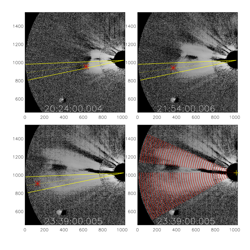
Figure 1: Examples of combined COR1 and COR2 images for three different observational times. The units are in pixel. The red asterisks mark the mean position of the leading edge from eight independent hand-traced positions for each time frame. All leading edge positions fall into the solid yellow cone of 10-degree width. In the bottom right panel, the red circular sections display the boundaries of the 39 shells inside which the mass is integrated.

A filament associated with a CME erupted at around 17:30 UT on November 10 2010 from an active region at Stoneyhurst coordinates 27^∘E, 10^∘N. The CME was then observed in the field of view of the coronagraphs onboard the Solar TErrestrial RElations Observatory (STEREO), and the coronagraphs onboard the Solar and Heliospheric Observatory (SOHO). In Figure 1, we present the combined COR1 and COR2 images at three selected time instances taken by STEREO A. In each case, pre-event background images were subtracted. Figure 1 therefore essentially shows the excess brightness produced by the CME. The dark region around the central latitude of 10${}^{{}^{\circ}}$N is due to the presence of a streamer in the pre-event image which dissolved after the eruption.

For later comparison, we hand-traced the leading edge position of the CME in a conventional way (e.g., Bein et al., 2011). As the leading edge, we define the most distant point of the CME cloud boundary. This boundary cannot always be located precisely because the CME brightness rises from a varying noise level at different distances from the center of the Sun. In order to determine the uncertainty, we repeated the tracking independently for eight times for each frame, and derived the mean and its variance of the leading edge position for each time frame. The mean leading edge positions were all located inside the yellow cone superposed in Figure 1. The averaged leading edge positions are marked by red asterisks. The leading edge distance versus time and its associated $3\sigma$ uncertainty are shown in Figure 2. The average speed of about 476 $\mathrm{kms^{-1}}$ yields a fairly close linear fit as shown by the straight line.

The simultaneous views of the CME from different perspectives provide a good constraint to determine its propagation direction in three dimensions. On November 10 2010, the two STEREO spacecraft were separated from the Earth by about 85^∘ each. Applying the graduated cylindrical shell forward modeling of Thernisien et al. (2009), we derived a propagation longitude about 27^∘E from the Sun-Earth line. This complies well with the location of the source region and implies a propagation at $\alpha=22^{\circ}$ behind the eastern plane-of-the sky of STEREO A.

3 Method

3.1 Mass estimate

A great advantage in the interpretation of white-light coronagraph images is the fact that the major part of its brightness signal is produced by Thomson scattering which depends linearly in the density $N_{e}$ of the scattering free electrons. The major non-Thomson scattered contributions like stray light and dust scatter are removed by subtracting the pre-event background image. The remaining image brightness then should show the CME density distribution produced by Thomson scattering alone. The details of this scattering process have already been developed more than fifty years and yield for the total image brightness in a given image pixel (Minnaert, 1930; van de Hulst, 1950; Billings, 1966).

$$B=B_{\odot}\frac{\pi\sigma_{e}}{2}\int_{\mathrm{LOS}}F(r,\chi,u)\;N_{e}(\mathbf{r})\;d\ell,$$ (1)

$$F(r,\chi,u)=2\frac{(1-u)C(r)+uD(r)}{1-u/3}-\frac{(1-u)A(r)+uB(r)}{1-u/3}\sin^{2}\chi$$

where $B_{\odot}$ is the mean solar brightness (MSB) of the solar disk, $\sigma_{e}$ is the coefficient of the differential Thomson scattering cross section and the parameter $u$ accounts for the solar disk limb darkening. The variables $A,B,C$ and $D$ are known functions (van de Hulst coefficients) of the distance $r$ of the scattering location from the solar center and $\chi$ is the respective scattering angle for a photon from the solar center to the observer. The integration has to be performed along the line-of-sight (LOS) defined by the effective view direction of the image pixel and $s$ is the geometrical distance along the LOS. We label the different LOSs by $\rho$, their closest distance to the Sun and set $s=0$ at this closest approach to Sun so that $r=\sqrt{\rho^{2}+s^{2}}$.

Since we do not know the true variation of $N_{e}$ along the LOS, Equation  1 cannot be evaluated without further assumptions. We adopt the approach proposed by Colaninno & Vourlidas (2009); Carley et al. (2012) which assumes the density is concentrated entirely in the mean propagation plane at an angle $\alpha$ off the plane-of-the-sky. Formally, this results in replacing $F(r,\chi,u)$ in (1) by $F(\rho/\cos\alpha,\pi/2-\alpha,u)$. For the limb darkening coefficient $u$ we adopt a value of 0.56.

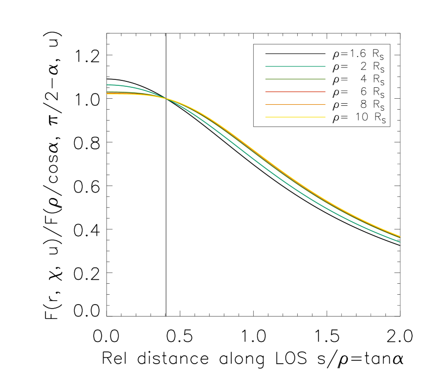
Figure 3: Thomson scattering weight function $F(r,\chi,u)$ along the line-of-sight distance $s$ for various LOS paths with distance of $\rho=1.6,2,4,6,8,10~{}R_{S}$ from the center of the Sun. The ordinate $F$ is normalized to the respective value at $s=\rho\tan\alpha$ where $\alpha$ is the angle of $22^{\circ}$ between the CME propagation plane and the POS. The abscissa is normalized by $\rho$. The vertical line represents $\alpha=22^{\circ}$.

In Figure 3 we show the variation of the weighting coefficient $F$ along a LOS at different distances $\rho$ from the solar center normalized to its value on the propagation plane at angle $\alpha$. If we knew the shape of the density distribution along the LOS at some distance $\rho$, the true column density $\int N_{e}\;d\ell$ differs from the approximate $\int\tilde{N}_{e}\;d\ell$ derived above by a factor obtained from the convolution of the known normalized density distribution along the LOS with the respective normalized weighting coefficient in Figure 3. The all-in-propagation-plane assumption yields

$$\int_{\mathrm{LOS}}F(r,\chi,u)\;N_{e}(\mathbf{r})\;d\ell=F(\frac{\rho}{\cos\alpha},\frac{\pi}{2}-\alpha,u)\int_{\mathrm{LOS}}\tilde{N}_{e}(\mathbf{r})\;d\ell$$

$$\text{or}\qquad\frac{\int_{\mathrm{LOS}}N_{e}(\mathbf{r})\;d\ell}{\int_{\mathrm{LOS}}\tilde{N}_{e}(\mathbf{r})\;d\ell}=[\int_{\mathrm{LOS}}\frac{F(r,\chi,u)}{F(\frac{\rho}{\cos\alpha},\frac{\pi}{2}-\alpha,u)}\;\frac{N_{e}(\mathbf{r})}{\int_{\mathrm{LOS}}N_{e}(\mathbf{r})\;d\ell^{\prime}}\;d\ell]^{-1}$$ (2)

We note that normalized weighting coefficient does hardly depend on the distance $\rho$ of the LOS from the solar center. I.e., a CME plasma volume propagating radially with a constant angle of propagation off the POS, i.e. with a constant $s/\rho$, receives the same LOS weighting. For an extended CME with an unknown LOS distribution, the correction we have to apply to the column density determined by the all-in-propagation-plane assumption does therefore hardly depend on $\rho$ if the CME propagates strictly radially.

We further note that a closer inspection shows that the $s$-dependence of the weighting coefficient in Figure 3 is due to the approximate $1/r^{2}$ dependence of the van de Hulst coefficients which reflects the decrease of the incident Sun light with distance from the solar center. The influence of the variation with scattering angle through the differential Thomson cross section is only minor.

3.2 Mass profiles and their uncertainty analysis

After the conversion of the excess brightness into the column electron density per pixel in the CME region, we can estimate the according column mass assuming a He²⁺/H⁺ composition of 10%. To analyze the mass transport inside the CME, we integrate the CME column mass density from each pixel over discrete shells of radius $r$ centered at Solar center to obtain mass $m(r,t)$ per unit length in radial direction at the times $t$ of the respective image. The discretization of radial shells is indicated in the bottom right panel of Figure 1. To define shells, we have divided the radial range from 1.6 to 14.8 R_S into 39 equal intervals and each 0.34 R_S wide. This discretization is large enough to raise the integrated mass in each shell significantly above the noise level, and small enough to sufficiently resolve the radial mass density distribution. In order to reduce the noise in the estimates of $m$ we limit the integration in latitude to the smallest possible sector which includes the CME. Note that we also excluded the narrow wedge near the center of the CME where the pre-event streamer disturbs the excess brightness.

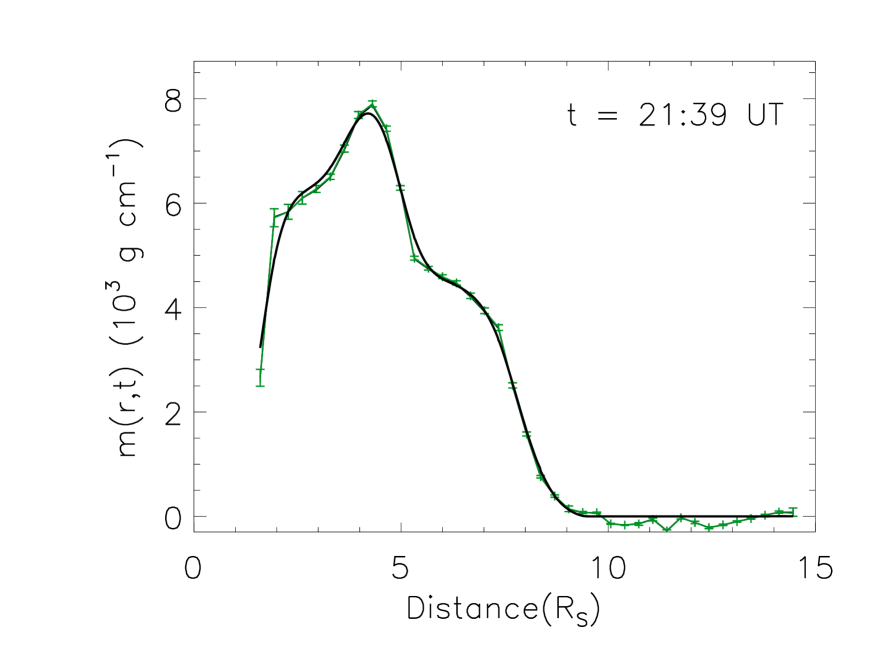
Figure 4: Example of the radial mass density profile at 21:39 UT. The green curve and the respective curve symbols were obtained from integrations of the image brightness. The error bars represent the $3\sigma$ of the integration results obtained for different selections of the CME sector and propagation angle. The black curve is a smoothed fit obtained from a smoothing spline.

There are two possible sources of systematic error in $m(r,t)$. One error in $m(r,t)$ may be due to the assumption in Equation 2 about the line-of-sight distribution of the CME mass, in particular due to a wrong longitudinal propagational angle $\alpha$. A second error in $m(r,t)$ may have been introduced by the somewhat arbitrary selection of the latitudinal integration boundaries. Choosing them too wide causes additional noise to be added to $m(r,t)$. To estimate these possible errors, we repeated the calculation of $m(r,t)$ twelve times for slightly different integration boundaries and also varied the propagation angle $\alpha$ within $22\pm 5^{\circ}$. As an example, in Figure 4 the average and $3\sigma$ uncertainty of the radial mass density profile from its twelve integrations at 21:39 UT is displayed in green.

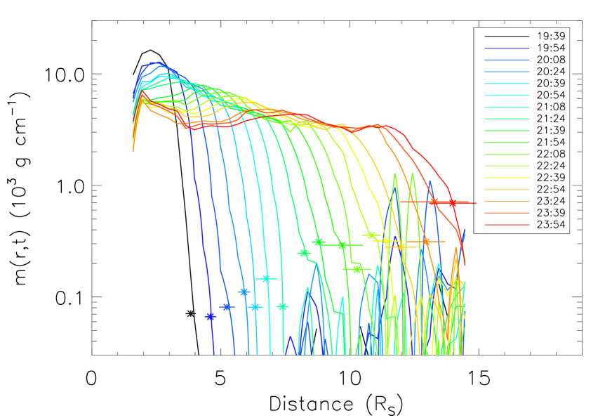
Figure 5: Time series of the mass profiles as a function of distance plotted in logarithm scale. The lines in different colors represent the mass profiles at different times. The color and time correspondence is shown in the upper right legend. The positions of the leading edge and their associated uncertainties are indicated by asterisks and errorbars.

Figure 5 displays the whole time series of mass density profiles $m(r,t)$ thus obtained. The colors from black to red indicate time $t$ in increasing order. On each curve, the asterisk marks the position of the hand-traced leading edge. We can see that the leading edge corresponds to finite, different mass densities which slightly increase with distance. There is still some residual CME mass ahead of the leading edge. The spikes in $m(r,t)$ at about $r>10R_{S}$ are due to the increasing noise in the coronagraph images towards the outer boundary of the field of view.

In order to derive other quantities from $m(r,t)$ and their uncertainty, we first fitted smoothing splines to $m(r,t)$ obtained so far. The amount of smoothing was controlled by the variance of the individual profiles from their average. One such smoothing spline is shown in black in Figure 4. Note that well ahead of the CME, $m(r,t)$ was set to zero before the smoothing. The mass measurements start to be sufficiently reliable at $\simeq 2~{}R_{S}$, about 0.5 $R_{S}$ above the COR 1 occulter.

3.3 Flow speed derivation

If we assume that there is no mass contribution from the pileup of the solar wind around the CME, the mass flow is described by a continuity equation

$$\frac{\partial{\rho}}{\partial{t}}+\boldsymbol{\nabla}\cdot(\rho\mathbf{v})=0.$$ (3)

The radial mass density profiles $m(r,t)$ which we have derived above are integrals of the volume mass density $\rho$ over cylinder surface sections which are spanned by the weighted LOS integration in one direction and heliographic latitude section in the other. Clearly, if $\mathbf{v}$ has only a radial component, the $\boldsymbol{\nabla}\cdot$-operation commutes with both integrations and Equation 3 could be transformed to

$$\frac{\partial{m}}{\partial{t}}+\frac{\partial}{\partial r}(mv_{r})=0$$ (4)

We expect that the major velocity component of the CME is indeed radial so that Equation 4 gives a good approximation to the evolution of the radial mass density $m$.

It is obvious that mass flow in latitudinal direction can be coped with by partial integration and does not change Equation 4 as long as the longitudinal integration boundaries were chosen wide enough to include the entire visible CME signal. The effect of a latitudinal component of the mass flow is more difficult to estimate. From Figure 3 we see immediately that a change of the propagation angle $\alpha$ or of the LOS density profile in the CME with distance $\rho$ could lead to a brightness change without changing the true column mass density. However, from many CME observations it has become evident that the non-radial components of the CME propagation is small. We will therefore in the following drop the index $r$ of $v_{r}$ in Equation 4 and assume this equation to be an adequate description for the evolution of $m$, neglecting possible changes in the mass density caused by the non-radial components of $\mathbf{v}$.

At first sight, Equation 4 seems of little value as long as $v(r,t)$ is not known. However since $m(r,t)$ is measured, it opens a chance to derive the velocity. Given that $m(r\rightarrow\infty,t)$ vanishes, an integration of Equation 4 over radius with variable lower bound yields

$$v(r,t)=-\frac{1}{m(r,t)}\;\frac{\partial}{\partial{t}}\int_{r}^{\infty}m(r^{\prime},t)dr^{\prime}$$ (5)

That is to say, at a given time, the total mass change beyond $r$ comes from the mass flow through the shell at $r$.

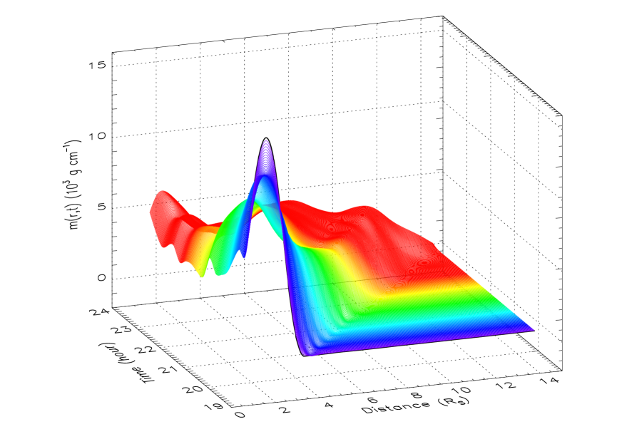
Figure 6: 2D cubic spline interpolation of mass profiles from 19:39 to 23:54 UT and between 1.6 and 14.8 R_S. The $X$ axis indicates the distance, and $Y$ axis indicates the time. The first mass profile at 19:39 UT is displayed in black, and the following mass profiles change their color with time from violet to red.

In Equation 5, the calculation of the velocity requires the time derivatives of mass profiles. To reliably calculate these derivatives, we interpolated the mass profiles using cubic splines. The result of such interpolations is presented in Figure 6. The first mass profile at 19:39 UT is displayed in black, and the following mass profiles change color with time from violet to red. The statistical error in $v(r,t)$ was obtained by repeating the calculation 300 times with mass density profiles $m(r,t)$ contaminated by random noise profiles of an amplitude which agrees to the standard deviation determined for $m(r,t)$. The variation in the resulting velocities was used to determine the error in $v(r,t)$. In such a way, we can derive an Eularian flow field within the CME at each interpolated space-time position. Some of the velocity profiles and associated errorbars at defined shell positions and at selected representative times are displayed in Figure 7. The solid curve in each panel is a quadratic fit to the derived velocity profile. Figure 8 shows an example of the time evolution of the Eulerian velocity at a given distance. We find that the Eulerian velocity decreases with time at all distances.

So far, we have ignored possible mass sources in the CME continuum equation 3 and 4. One such possibility which has been discussed is the pile up of solar wind mass in front of a fast propagating CME. We see similar density enhancements ahead of fast solar wind streams where they run into the warped up current sheet. Formally, this could be taken into account by adding a source term in Equation 4. The effect on the velocity derived can be seen straight forwardly. If a source is present, then

$$\frac{\partial}{\partial t}m=-\frac{\partial}{\partial r}(vm)+s(r,t)$$

$$\text{Set}\qquad f(r,t)=\int^{r}s(r^{\prime},t)dr^{\prime}\quad\text{then}$$

$$\frac{\partial}{\partial t}m=-\frac{\partial}{\partial r}(vm)+\frac{\partial}{\partial r}f=-\frac{\partial}{\partial r}((\underbrace{v-f/m}_{v^{\prime}})m)$$

Hence, the source term is absorbed in the flow velocity which we obtain from Equation 5. For example if there is mass pile-up in front of the CME, $f$ should grow near the front side of the CME from zero to the piled-up mass well ahead of the CME. This should lead to a strong decrease of the velocity $v^{\prime}$ since, at the front side of the CME, $m$ drops with distance and the velocity contamination $f/m$ increases even stronger than $f$ alone. Therefore a mass pile-up should show as a decrease in the velocity profile near the CME front. In Figure 7 we see that the velocity at the CME front is persistently about 450-500 km s^-1. Note that the error in the most distant velocity estimate has a relatively large uncertainty because it was obtained in Equation 5 from a division by a small mass density $m(r,t)$.

3.4 Validation of flow speeds

To check the consistency of the velocity $v(r,t)$ derived above we have used it in the continuity equation, i.e., Equation 4 to predict the radial mass density profile $m(r,t_{j})$ from a given initial value $m(r,t_{j-1})$. Both times $t_{j-1}$ and $t_{j}$ were chosen to coincide with the observational times the coronagraph images were taken so that the respective mass density profiles were those obtained directly from the integration of image data. The continuity equation was integrated by a straight forward Lax-Wendroff scheme. The boundary condition varies linearly from $m(r_{0},t_{j-1})$ to $m(r_{0},t_{j})$ at each time step.

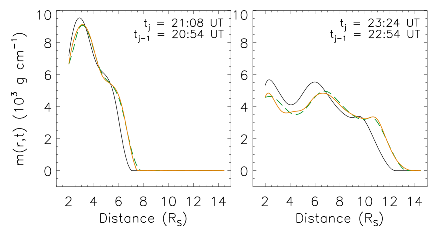
Figure 9: Comparison of measured and calculated mass profiles. The solid lines in black and orange show the measured $m(r,t)$ at times $t_{j-1}$ and $t_{j}$. The dashed line in green is the $m(r,t)$ at $t_{j}$ calculated from the profile at $t_{j-1}$.

Figure 9 shows examples at two pairs $t_{j-1}$ and $t_{j}$ of successive image times. The solid black and orange lines are the measured mass density profiles at $t_{j-1}$ and $t_{j}$, respectively. The dashed green line is the profile calculated from $t_{j-1}$ to $t_{j}$ using the flow speeds $v(r,t)$ derived in the previous subsection. It can be seen that the predicted and measured mass density profiles fit fairly well.

4 Results

The knowledge of the velocity and mass distribution allows us to study the CME kinetics in much more detail than was possible in many previous investigations. However, $v(r,t)$ is the velocity is in the Eulerian frame with $r$ and $t$ considered independent variables which is sometimes difficult to interpret. It is more instructive to see the CME mass transport in the frame of the individual CME mass element.

4.1 Lagrangian trajectories and leading edge positions

A change of Equation 4 to the Lagrangian frame is achieved first by integrating the velocity to the Lagrangian or material path of a mass element

$$\frac{\partial}{\partial t}R(t,t_{0})=v(r=R(t,t_{0}),t)\quad\text{with initial condition}\quad R(t_{0},t_{0})=r_{0}$$ (6)

In this formulation, the paths $R$ are labeled according to the time $t_{0}$ (2nd argument) when they pass the distance $r_{0}\simeq 2\,R_{\odot}$ where we start our velocity derivation.

Along these paths the advected mass density $m(r=R(t,t_{0}),t)$ then changes in time according to

$$\frac{dm}{dt}=-m\frac{\partial v}{\partial r}(r=R(t,t_{0}),t)$$ (7)

The error bars assigned to each path represent the estimated uncertainty obtained again by repeated integrations of Equation 6 of the average flow speed perturbed with random noise profiles of amplitude in agreement with the standard deviation of $v(r,t)$.

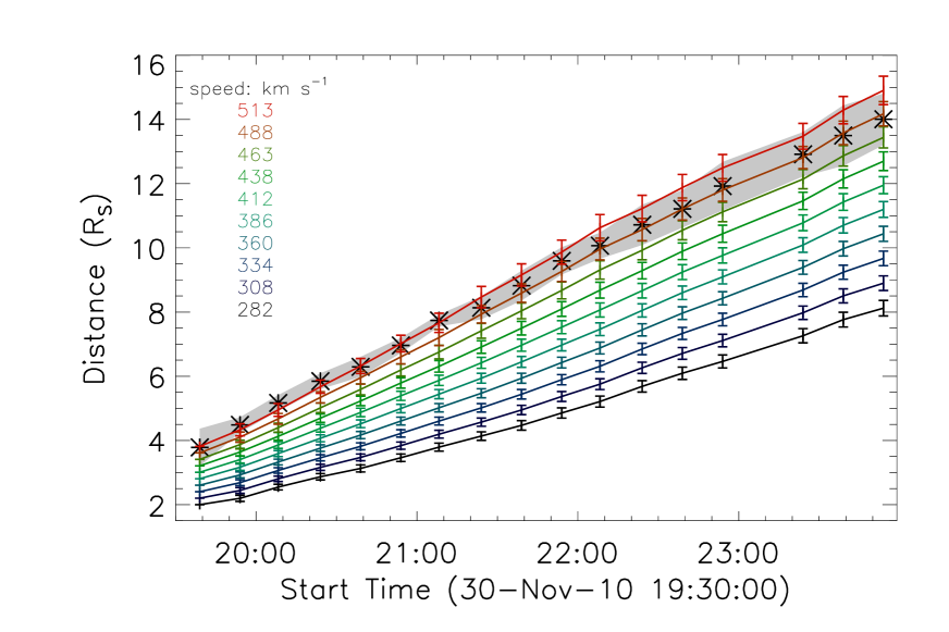
Figure 10: Some Lagrangian trajectories derived from the Eularian velocity profiles. At their starting time 19:39 UT, they were equally distributed within the CME region between 2 and 3.8 $R_{S}$. The error bars are derived from the uncertainties of the velocity profiles. The asterisks and the shaded gray color mark the leading edge positions and their associated uncertainties. The corresponding averaged Lagrangian speeds are indicated in the left in the same color as the respective trajectories.

From the derived Eularian velocity field in the last section, it is possible to derive the Lagrangian path of a mass element starting from $r_{0}$ at time $t_{0}$. In Figure 10, we present the Lagrangian path of 10 mass elements starting at 19:39 UT. At 19:39 UT, the CME mass covers a range from 2 to 3.8 R_⊙. The selection of ten mass elements is to make the errorbars of the trajectories distinguishable between neighboring trajectories, and at the same time sufficiently resolve the properties of different trajectories. For the CME studied here, each mass element propagates at almost a constant Lagrangian velocity. The height-time diagram of the Lagrangian paths in Figure 10 closely resembles a fan, however, each Lagrangian path (and those in between) carrying a different amount of mass density. If we approximate these velocities by exact constants, it is easily seen that $\partial v/\partial r\propto 1/t$ and the mass density along a Lagrangian path decreases as $\propto 1/R$.

Any significant derivation of the Lagrangian path from a straight line indicates either an physical acceleration $dv/dt$ of CME masses or, as discussed in section 3.3, the presence of a mass source. In the example studied here we conclude from the constancy of the Lagrangian trajectories that there is possibly no evidence for either of the two.

We note that the asterisks, which represent the radial advance of the leading edge are attached to the fastest Lagrangian path in the beginning but slightly fall behind systematically at later times. The leading edge we have picked by visual inspection (see Figure 2) may therefore not exactly correspond to a material path as the name suggests. It seems that as the CME front dims away at increasing distance from the Sun, there is a tendency to place the leading edge position further inward where the image brightness is more enhanced.

Another interesting aspect of Figure 10 is the possibility to extrapolate the Lagrangian paths backwards. We find that the fastest path with a mean velocity of 521 $\mathrm{km\,s^{-1}}$ intersects the solar surface at 18:35 UT, about one hour after a flare in the EUV images indicates the initiation of the eruption at $t_{\mathrm{flare}}=17:30$ UT. The slower velocity paths extrapolate to the surface at increasingly later times, the slowest velocity path with a mean of 283 $\mathrm{km\,s^{-1}}$ intersects $r=1$ at 18:58 UT. A mass element experiencing approximately a constant acceleration between some time $t_{\mathrm{start}}$ and time $t_{\mathrm{end}}$ will propagate afterwards on a Lagrangian path which intersects the solar surface at $(t_{\mathrm{start}}+t_{\mathrm{end}})/2$, irrespective of the strength of the acceleration. If this simple model holds true, the fast masses (red trajectories in Fig. 10) must have been accelerated earlier than the slow masses (dark blue trajectories).

4.2 CME energy

Usually the kinetic energy of a CME is estimated by simply using its total mass and the leading edge speed. This ignores the extended distribution of CME mass and velocity. For the CME we analyzed here, we see systematically lower speeds with increasing distance from the leading edge. Therefore, the conventional approach probably tends to overestimate the kinetic energy of a CME.

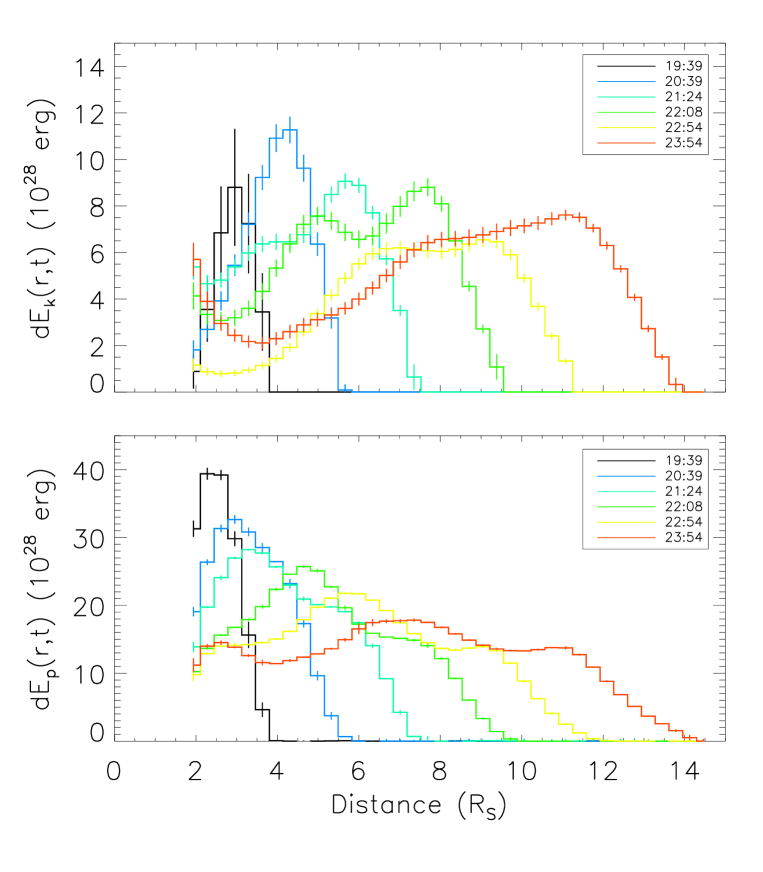
Figure 11: Profiles of kinetic energy and gravitational potential energy in each shell at a few representative times. The energy profiles at different colors represent the profiles at different times. The color-time correspondence is shown in the upper right legend.

In the upper panel of Figure 11, we show the kinetic energy of the CME between successive shells at $r_{i}$ and $r_{i+1}$ at a few selected times

$$dE_{\mathrm{k}}(r_{i},r_{i+1},t)=\int_{r_{i}}^{r_{i+1}}\frac{m(r,t)}{2}v^{2}(r,t)\;dr.$$ (8)

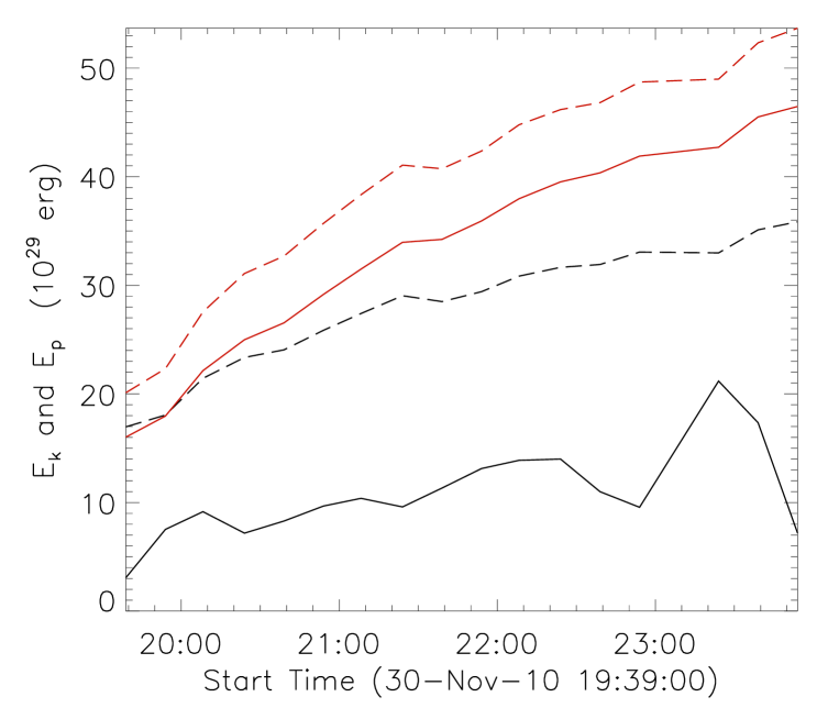
Figure 12: Total kinetic energy and gravitational potential energy of the CME in our FOV are shown by black and red solid lines, respectively. The dashed lines represent the respective conventional energy estimates derived using the total mass and the leading edge motion.

The non-uniformity of the kinetic energy of CME shells can be clearly seen. In Figure 12 the time evolution of the total kinetic energies of the entire CME $E_{k}$ are marked in black. The values derived with the conventional method indicated by the dashed line can be four times larger than the values obtained with our more refined method indicated by the solid line. This large discrepancy mainly comes from the $v^{2}$ term in Equation 8.

Another energy we estimated is the gravitational potential energy above the solar surface according to:

$$dE_{\mathrm{p}}(r_{i},r_{i+1},t)=\int_{r_{i}}^{r_{i+1}}m(r,t)g_{\odot}\frac{R_{S}}{r}(r-R_{S})\;dr.$$ (9)

The potential energy of each shell at the same selected times as the kinetic energy is illustrated in the lower panel of Figure 11. The non-uniformity of the potential energy is also evident. The total potential energy $E_{p}$ plotted in red in Figure 12 reveals that $E_{p}$ estimated using total mass and leading edge distances may also overestimate the true value. The discrepancy between $E_{p}$ derived with these two different methods is much smaller, compared with that of $E_{k}$.

5 Conclusions and Discussions

We have presented a new approach to analyze the mass evolution and advection in a CME. It yields the radial mass density distribution and, as a derived quantity, the radial velocity profile and its temporal evolution. This represents much more detailed information than previous mass evolution diagrams. As another advantage, our analysis is much less dependent on subjective manual interference than the traditional tie-pointing of the leading edge.

Our analysis allows us to detect acceleration also inside the CME and, at least indirectly, from implausible velocity profiles to conclude about the existence of CME mass sources in the solar wind, e.g., by pile-up. These conclusions could not be drawn from the conventional total mass evolution plots. In the present study of a slow CME, we did not find a speed decrease in the profiles which could indicate such a pile-up expected ahead of CME. In future we will apply our analysis to a fast CME where such a pile-up is more probable. In this case, we will include a pile-up induced source term in the continuity equation.

The velocity profiles obtained are compatible with a self-similar propagation of the CME between 2 and 15 R_S, at least as far as the radial advection of CME mass density is concerned. From the mass and velocity profiles inside the CME we can determine where the most mass and kinetic energy is stored. This could by forward extrapolation help to forecast effective travel times which do not always seem to agree well with the speed of the leading edge. By a careful backwards extrapolation towards the source it might in some cases become possible to explore the initial distribution of the CME mass in the corona. E.g. it could tell, how much of the CME mass originates in the chromosphere or in protuberances and which portion is delivered by streamer plasma at higher altitudes (Kramar et al., 2009).

It is also our aim to extend the profiles beyond the FOV of COR2 and use the HI1 and HI2 coronagraph data of STEREO. From in-situ observations of a solar wind transient, the speed at different positions of an ICME can be measured directly. As an outlook, we plan to compare the speed distribution in the FOV of COR to HI with the mass flow observed in-situ at 1 AU. Another extension of our study would be to apply it to the observations from the two view directions of the STEREO spacecraft. The possible three dimensional distributions of mass and velocity profiles would be constrained by their independent measurements from two view points.

Figure 2: The distance-time plot of the leading edge and a corresponding linear fit. The symbols represent the mean and the $3\sigma$ uncertainties of the leading edge distance. An averaged speed and its $3\sigma$ uncertainty derived from the linear fit is indicated in the upper part.

Figure 7: The distribution of flow speed with distance for six selected time instances. The error bars in each panel were derived from the uncertainties of the mass profiles.

Figure 8: An example of the evolution of flow speed with time at a distance of $r=3.96~{}R_{S}$. The error bars are the same as in Figure 7.

References

- Bein et al. (2011) Bein, B. M., Berkebile-Stoiser, S., Veronig, A. M., et al. 2011, ApJ, 738, 191
- Bein et al. (2013) Bein, B. M., Temmer, M., Vourlidas, A., Veronig, A. M., & Utz, D. 2013, ApJ, 768, 31
- Billings (1966) Billings, D. E. 1966, A guide to the solar corona
- Carley et al. (2012) Carley, E. P., McAteer, R. T. J., & Gallagher, P. T. 2012, ApJ, 752, 36
- Colaninno & Vourlidas (2009) Colaninno, R. C., & Vourlidas, A. 2009, ApJ, 698, 852
- Kramar et al. (2009) Kramar, M., Davila, J., Xie, H., & Antiochos, S. 2009, in AAS/Solar Physics Division Meeting, Vol. 40, AAS/Solar Physics Division Meeting nr 40
- Mierla et al. (2011) Mierla, M., Chifu, I., Inhester, B., Rodriguez, L., & Zhukov, A. 2011, A&A, 530, L1
- Mierla et al. (2009) Mierla, M., Inhester, B., Marqué, C., et al. 2009, Sol. Phys., 259, 123
- Minnaert (1930) Minnaert, M. 1930, Zeitschrift fuer Astrophysik, 1, 209
- Thernisien et al. (2009) Thernisien, A., Vourlidas, A., & Howard, R. A. 2009, Solar Physics, 256, 111
- van de Hulst (1950) van de Hulst, H. C. 1950, Bulletin of the Astronomical Institutes of the Netherlands, 11, 135
- Ventura et al. (2002) Ventura, R., Spadaro, D., Uzzo, M., & Suleiman, R. 2002, A&A, 383, 1032