Frequency-Dependent Dispersion Measures and Implications for Pulsar Timing

Abstract

We analyze the frequency dependence of the dispersion measure (DM), the column density of free electrons to a pulsar, caused by multipath scattering from small scale electron-density fluctuations. The DM is slightly different along each propagation path and the transverse spread of paths varies greatly with frequency, yielding arrival time perturbations that scale differently than the inverse square of the frequency, the expected dependence for a cold, unmagnetized plasma. We quantify DM and pulse-arrival-time perturbations analytically for thin phase screens and extended media and verify the results with simulations of thin screens. The rms difference between DMs across an octave band near 1.5 GHz $\sim 4\times 10^{-5}\,{\rm pc\ cm^{-3}}$ for pulsars at $\sim 1$ kpc distance. Time-of-arrival errors resulting from chromatic DMs are of order a few to hundreds of nanoseconds for pulsars with DM $\mathrel{\hbox{\hbox to0.0pt{\hbox{\lower 4.0pt\hbox{$\sim$}}\hss}\hbox{$<$}}}30$ pc cm^-3 observed across an octave band but increase rapidly to microseconds or larger for larger DMs and wider frequency ranges. Frequency-dependent DMs introduce correlated noise into timing residuals whose power spectrum is ‘low pass’ in form. The correlation time is of order the geometric mean of the refraction times for the highest and lowest radio frequencies used and thus ranges from days to years, depending on the pulsar. We discuss the implications for methodologies that use large frequency separations or wide bandwidth receivers for timing measurements. Chromatic DMs are partially mitigable by using an additional chromatic term in arrival time models. Without mitigation, our results provide an additional term in the noise model for pulsar timing; they also indicate that in combination with measurement errors from radiometer noise, an arbitrary increase in total frequency range (or bandwidth) will yield diminishing benefits and may be detrimental to overall timing precision.

1. Introduction

Pulsar arrival times with sub-microsecond accuracy are required for the detection of nanohertz-frequency gravitational waves using pulsar timing arrays (e.g. Foster & Backer, 1990) and have payoffs in related areas, such as precision tests of theories of gravity Kramer et al. (2006), determination of neutron star masses Antoniadis et al. (2013), and characterization of microstructure in the interstellar medium (ISM) Isaacman & Rankin (1977).

A pulse’s time of arrival (TOA) includes a group delay term, $t_{\rm DM}(\nu)=K\nu^{-2}\rm DM$, where the dispersion measure (DM) is the integral of the electron number density along the line of sight, $\nu$ is the frequency and the constants are $K=cr_{e}/2\pi$ and the classical electron radius $r_{e}$. A key step in arrival-time analysis is the removal of the dispersion term. Estimates of DM  based on TOA differences between two or more frequencies show that DM is epoch dependent for most well-studied pulsars (Isaacman & Rankin, 1977; Hamilton et al., 1985; Cordes et al., 1990; Phillips & Wolszczan, 1991; Backer et al., 1993; Kaspi et al., 1994; Ilyasov et al., 2005; Ramachandran et al., 2006; Demorest et al., 2013; Keith et al., 2013; Petroff et al., 2013; Fonseca et al., 2014). Temporal variations include a slow, systematic trend as a pulsar moves toward or away from us along with stochastic variations from pulsar motion that causes the line of sight to sample electron-density fluctuations on a variety of scales.

In this paper we show that the DM is also frequency dependent because the ISM is sampled differently due to multipath scattering. The DM along each ray path is slightly different and the size of the ray-path bundle increases monotonically with decreasing frequency, leading to a net difference in dispersive delays in the sum over all ray paths. The variation with frequency of $\rm DM(\nu,t)$ stays constant for a refraction time, which is the time scale for the ray-path bundle to move by its transverse extent and can range from hours to years (Rickett et al., 1984; Stinebring et al., 2000). Our analysis includes the general case of an arbitrary medium described by a wavenumber spectrum that varies along the line of sight (LOS). We give specific results for the case of a thin screen and for a medium with homogeneous statistics for electron-density variations. We compare analytical results with simulations of scattering and dispersion. Our analysis is for the strong scattering regime where all of the flux from a pulsar is scattered. In the summary and conclusions section we briefly discuss the weak scattering regime and its role in precision timing.

Our results complement those of Lam et al. (2015), who quantified TOA errors that result from estimates for DM that make use of timing observations at different frequencies that are not made on the same day. Here we show that even simultaneous multi-frequency measurements yield TOA errors because the DM varies with frequency.

Section 2 derives the basic effect and gives specific results for a thin screen and for a medium with uniform statistics. Section 3 concerns implications for pulsar timing methodology and precision. Section 4 discusses our results and summarizes our conclusions. In Appendix A we derive scattering quantities and in Appendix B we derive the RMS two-frequency variation of DM.

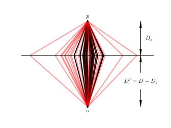
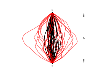
Figure 1.— Geometries for scattering from a thin screen (left) and filled medium (right). Black lines show simulated ray paths at frequency $\nu$ and red lines are for frequency ${\nu^{\,\prime}}=\nu/2$. The pulsar-observer distance is $D$. The thin screen is at a distance $D_{s}$ from the pulsar at $p$ and ${D^{\prime}}=D-D_{s}$ from the observer at $o$.

2. Dispersion Measure Variations in Time and Frequency

There are several underlying causes for temporal variations of DM but only electron density fluctuations in the ISM produce a large enough frequency dependence to be important in precision timing . For a spatially uniform $n_{e}$, the DM  is independent of frequency and any epoch dependence comes from changes in the pulsar distance $D$. Motions of the pulsar and Earth with a combined velocity $100V_{100}$ km s^-1 parallel to the LOS yield $\delta\rm DM\sim 3\times 10^{-6}~{}{\rm pc~{}cm^{-3}}V_{100}t_{\rm yr}n_{e_{0.03}}$ over $t_{\rm yr}$ years for a typical average electron density $n_{e}=0.03$ cm^-3. Linear trends in DM are indeed seen (e.g. Keith et al., 2013) but this effect is likely to be frequency independent.

Chromatic DMs result from multipath propagation caused by diffraction and refraction from interstellar electron density variations. The effect we identify is not due to geometrical path-length differences alone. Gravitational lensing, for example, could produce multiple ray paths through a medium with constant electron density, but the resulting DM variations would be negligible ($\mathrel{\hbox{\hbox to0.0pt{\hbox{\lower 4.0pt\hbox{$\sim$}}\hss}\hbox{$<$}}}10^{-16}$ pc cm^-3) given observational bounds on time delays between paths $<1~{}\mu s$. Moreover, they would be achromatic.

Density variations exist over a wide range of length scales from kpc to around $10^{3}$ km (e.g. Armstrong et al., 1995) and the smaller ones are responsible for multipath propagation. The DM varies slightly between ray paths and the cross-sectional area of the ray-path bundle at any position along the LOS is strongly frequency dependent, $\propto\nu^{4}$. Density microstructure therefore plays two roles: causing multipath propagation and providing variable path integrals of the electron density. Figure 1 shows frequency-dependent ray paths for a thin scattering screen and for a medium that fills the volume between us and a pulsar; it also defines some of our notation.

We model the electron density to be $n_{e}({{\bf x}})=\overline{n}_{e}({{\bf x}})+\delta n_{e}({{\bf x}})$, where $\overline{n}_{e}({{\bf x}})$ is a constant local mean and $\delta n_{e}({{\bf x}})$ is the zero-mean fluctuating part described by a wavenumber spectrum $P_{\delta n_{e}}({\bf q},z)$ that can vary slowly along the line of sight ($z$-axis). We adopt a power-law wavenumber spectrum of the form

$$P_{\delta n_{e}}({\bf q},z)=\rm C_{n}^{2}(z)q^{-\beta},\quad\quad q_{0}\leq q\leq q_{1}.$$ (1)

The dependence on only the magnitude of ${\bf q}$ is a simplifying assumption, discussed further in the next subsection, that conflicts with some observations that show elliptical scattered images but is consistent with others that show circular images.

The electromagnetic phase perturbation $\phi$ from the index of refraction in a cold plasma is proportional to the integrated electron density along a ray path (Rickett, 1990, Appendix A, Eq. A5),

$$\phi({{\bf x}})=-\lambda r_{e}\int_{\rm{}_{ray}}\!\!\!\!\!dz\,n_{e}({{\bf x}^{\prime}}(z),z),$$ (2)

where ${{\bf x}}$ is the transverse location in the observation plane a distance $D$ from the pulsar while ${{\bf x}^{\prime}}$ is a transverse vector at a location $z$ along the LOS.

For any single ray path the phase perturbation corresponds to a dispersive time delay $t_{\rm DM}=(1/2\pi)(d\phi/d\nu)$ characterized by a dispersion measure, $\rm DM=-\phi/\lambda r_{e}$. Converting $\lambda r_{e}$ to DM units at 1 GHz yields a natural value for one radian of phase, $\delta\rm DM_{1}=3.84\times 10^{-8}$ pc cm^-3. Since we know that pulsars are scattered significantly at radio frequencies, phase perturbations $\phi_{F}$ on the Fresnel scale $r_{F}=\sqrt{\lambda D/2\pi}\sim 10^{11}$ cm are necessarily many radians. The Fresnel scale corresponds to less than one day of transverse motion for pulsar velocities $\sim 100$ km s^-1. We therefore expect DM to vary by large multiples of $\delta\rm DM_{1}$ on time scales of weeks and longer because the RMS phase grows with increasing time span for media with a spectrum like that in Eq. 1. By similar reasoning, we expect frequency-dependent DM differences $\gg\delta\rm DM_{1}$ because ray paths at widely spaced frequencies have separations much larger than the Fresnel scale.

Figure 2 shows the manifestation of chromatic DMs in simulated arrival times vs. frequency. The curve in the main part of the figure is dominated by the mean $\rm DM=10$ pc cm^-3. The inset shows the deviations from the mean curve from 0.4 to 0.8 GHz for 100 realizations of a phase screen with $\phi_{F}=30$ rad, demonstrating the spread in arrival times over $\pm 1~{}\mu s$ at the lowest frequency.

2.1. Simulations of Phase Screens and Ray-path Averaging

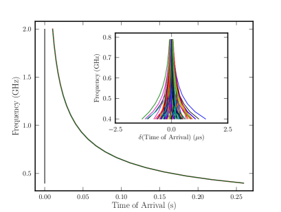
Figure 2.— Trajectories of a dispersed pulse in the time-frequency plane for 100 realizations using a phase screen with $\phi_{F}=30$ rad at 1 GHz. The dedispersed trajectories are shown aligned with $t=0$, and the inset shows details of the dedispersed trajectories for the lower part of the frequency band.

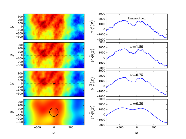
Figure 3.— Phase screen for electron-density fluctuations with a Kolmogorov wavenumber spectrum that has $\phi_{F}=5$ rad RMS phase variation on the Fresnel scale. The $x$ and $y$ coordinates are in units of the Fresnel scale at 1 GHz and the RMS phase difference grows as $\Delta^{5/6}$ between two points separated by $\Delta=[(\Delta x)^{2}+(\Delta y)^{2}]^{1/2}$. For a velocity $V_{x}=100$ km s^-1, each sample corresponds to 0.28 d and the entire span of $x$ corresponds to 2 yr. Left: phase screens without (top) and with spatial smoothing. The bottom three panels are for frequencies of 1.5, 0.75, and 0.3 GHz, as labeled in the right hand panels. Plotted circles (barely discernible in the middle two frames) are projected scattering-disk sizes and represent the region with $1/e$ radius on the phase screen that is averaged to produce the DM difference at any given epoch and frequency. The area scales as $\nu^{22/5}$. Right: phase variations corresponding to trajectories along the dashed lines in the left-hand panels. The 1D curves are not smoothed versions of $\phi(x)$ in the top panel because the smoothing is two dimensional.

Phase screens were simulated using approaches similar to those presented in Cordes et al. (1986); Coles et al. (1987); Foster & Cordes (1990); Hu et al. (1991) and Coles et al. (2010). An array in the wavenumber domain was filled with white, Gaussian, Hermitian noise shaped by the square root of the ensemble-average power spectrum. A 2D inverse FFT yields the phase screen. To include low-frequency components excluded by the FFT, we separately added wavenumber components with periods up to three times the array size in each direction. Phase fluctuations were scaled to a specified Fresnel phase at a fiducial frequency, which we took to be 1 GHz. We exploited the scale invariance of the phase fluctuations by simulating a set of phase screens for small values $\phi_{F}=5$ rad, which require fairly small 2D arrays, and rescaling to larger values. We verified that this procedure was correct by explicitly simulating a few large phase screens.

Figure 3 shows an example phase screen and the averaging areas projected onto the screen for a 5:1 range of frequencies. DM differences are due solely to the change in averaging area. At different epochs the averaging areas sample different parts of the screen, producing stochastic variations in DM that are correlated over the time it takes for the averaging area to move by its diameter. The difference in DM between a pair of frequencies is constant over the correlation time for the higher of the two frequencies, which has the smaller scattering disk.

Figure 4 shows realizations of $\rm DM(\nu,t)$ at eight frequencies (left-hand panel) obtained using a phase screen for a Kolmogorov spectrum ($\beta=11/3$). The figure demonstrates that variations in DM on long time scales are similar over a 5:1 frequency range, but differ on short time scales, with a more rapid variation at higher frequencies. The variation in DM has a very ‘red’ power spectrum and is a non-stationary process. However, the DM differences between pairs of frequencies (right-hand panel) have flatter spectra and show characteristic time scales associated with ray-path smoothing. The autocorrelation widths are roughly the geometric mean of the smoothing lengths at each pair of frequencies. These smoothing lengths correspond to the times scales of refractive scintillations. Consequently the time series of DM differences between a pair of frequencies is a ‘red’ process with a Gaussian-like power spectrum. Figure 5 shows power spectra of DM variations at two radio frequencies (red curves) and power spectra of DM differences for several pairs of frequencies (black curves).

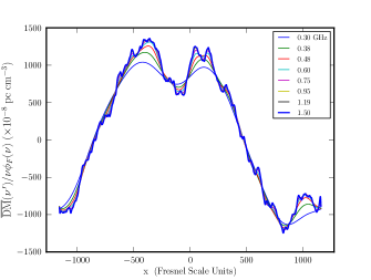
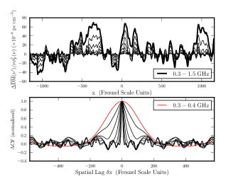
Figure 4.— (Left) A single realization showing $\rm DM(t)$ at 8 frequencies from 0.3 GHz (red) to 1.5 GHz. The DM values have been normalized by the quantity $\nu_{1}\phi_{F}(\nu_{1})$ for $\nu_{1}=1$ GHz. (Right) Top panel: time series of $\rm DM(t)$ differences between 1.5 GHz and all lower frequencies. The thinnest lines are for the frequencies nearest 1.5 GHz and the thickest for 0.3 GHz. Bottom panel: normalized autocorrelation functions of the difference time series in the top panel along with the ACF of the DM difference between the two lowest frequencies (0.4 and 0.5 GHz, red). The main lobe of each ACF near zero lag represent the characteristic spatial scale of the DM difference. Spatial units can be converted to time units using $\Delta x=V_{x}\Delta t$. Using 100 km s^-1 velocity and a Fresnel scale for 1 GHz and 1 kpc distance, one spatial unit corresponds to 0.14 d.

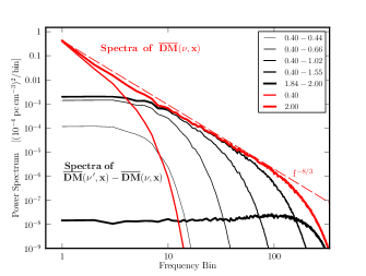
Figure 5.— Power spectra of dispersion measure variations $\overline{\rm DM}\ (\nu,{{\bf x}})$ (red lines) and of dispersion-measure differences between frequencies $\overline{\rm DM}({\nu^{\,\prime}})-\overline{\rm DM}(\nu)$ as designated in the legend. The results are based on 1000 realizations of a screen with $\phi_{F}=30$ rad and a Kolmogorov spectrum, which yields a power spectrum for DM variations with a $-8/3$ slope, as indicated by the dashed line.

2.2. Frequency-Dependent Averaging Over Ray Paths

The measurable DM is an average over all ray paths that reach Earth. At any location along the integration path, the narrow ray-path bundle spans a transverse area described by ${{\bf x}}(z)$ that also depends on frequency. We define a frequency-dependent averaging function ${A_{\nu}({{\bf x}},z)}$ that is normalized to unit area, $\int d{{\bf x}}\,{A_{\nu}({{\bf x}},z)}=1$. The averaged DM is the LOS integral of the convolution of the averaging function with the electron density,

$$\overline{\rm DM}(\nu,{{\bf x}})=\langle\rm DM({{\bf x}})\rangle+\int_{0}^{D}dz^{\,\prime}\int_{-\infty}^{\infty}d{{\bf x}^{\prime}}\,{A_{\nu}({{\bf x}}-{{\bf x}^{\prime}},z^{\,\prime})}\delta n_{e}({{\bf x}^{\prime}},z^{\,\prime}),$$ (3)

where the frequency-independent term $\langle\rm DM({{\bf x}})\rangle$ is the ensemble average (denoted by angular brackets) of the integrated electron density ${\overline{n}_{e}}$. An appropriate averaging function ${A_{\nu}({{\bf x}},z)}$ is the scattered image of the pulsar that generally also includes refraction, which offsets the image from the actual pulsar direction. The scattered image $I({\mbox{\boldmath$\theta$}})$ is the two-dimensional Fourier transform of the visibility function $\Gamma({\mbox{\boldmath$b$}})=\exp(-D_{\phi}({\mbox{\boldmath$b$}})/2)$, where $D_{\phi}$ is the phase structure function defined in Appendix A. The phase structure function is the mean-square phase difference of the wavefield between two points separated by distance $b$ transverse to the LOS. In accordance with our assumptions about the spectrum $P_{\delta n_{e}}$, $D_{\phi}$ depends only on the magnitude of $b$.

In the most general case, the image can be elliptical or split into multiple subimages. Elliptical images have been seen for some scattered sources while others are nearly axisymmetric. An extreme case for a nearby pulsar was given by Brisken et al. (2010), who infer an image that is Gaussian-like but with $\sim 1$ % of the flux spread into a long, linear image with high aspect ratio. Refraction angles are evidently smaller than scattering angles based on the lack of significant angular wandering in VLBI images. In addition, for media having wavenumber spectra like those that are consistent with a wide range of scattering and scintillation measurements, refraction angles are expected to be small. Since our goal is to describe the basic phenomenon of frequency-dependent DMs rather than address all possible varieties of scattering and refraction, the essential features are captured with a simplified approach that allows analytical tractability. The calculation undertaken here simply looks at the difference in electron column density that results from the frequency dependence of the ray-path bundle that samples the medium. The calculation of the arrival-time difference does not take into account additional delays that result from lateral shifts of the ray-path bundle due to refraction or changes due to focusing and defocusing by quadratic phase changes. We emphasize therefore that our results likely underestimate the total frequency-dependence of DMs.

First we make some simple estimates of DM variations. From the phase structure function $D_{\phi}(b)$ we show that the RMS variation of $\overline{\rm DM}$ across the screen-averaging area scales as the square of the RMS Fresnel phase $\phi_{F}$, and in the next section we derive a precise scaling law for the RMS difference in $\overline{\rm DM}$ between two frequencies. The DM structure function is equal to $D_{\phi}(b)/(\lambda r_{e})^{2}$. Without any ray-path averaging, it can be written in terms of the RMS Fresnel phase as

$$D_{\rm DM}(b)=\frac{\phi_{F}^{2}}{(\lambda r_{e})^{2}}\left(\frac{b}{r_{F}}\right)^{\beta-2}.$$ (4)

Averaging over ray-paths yields an RMS DM difference obtained by averaging the DM structure function over a circular area with radius $\sigma_{X}\sim r_{F}\phi_{F}^{2/(\beta-2)}\geq r_{F}$ (which can be derived using Eq. A8, A9, A12 and B8). This prescription is applicable only for moderate to strong scattering with $\phi_{F}\mathrel{\hbox{\hbox to0.0pt{\hbox{\lower 4.0pt\hbox{$\sim$}}\hss}\hbox{$>$}}}1$. We discuss weak scattering in Section 3.4. The averaging radius is essentially the ‘refraction’ scale for refractive scintillations, which is equal to the observed scattering angle projected onto the screen at a distance $D^{\prime}$ from Earth (c.f. Figure 1); it is also the minimum scale for DM variations. This gives for $\nu$ in GHz,

$$\overline{\rm DM}_{\rm rms}\sim\phi_{F}^{2}/\lambda r_{e}\sim 3.84\times 10^{-8}\,{\rm pc~{}cm^{-3}}\ \nu\phi_{F}^{2}.$$ (5)

The scaling of $\overline{\rm DM}_{\rm rms}$ as the square of $\phi_{F}$ arises because the screen phase and the averaging radius are both approximately linear in $\phi_{F}$. The Fresnel phase scales with frequency as $\nu^{-17/12}$ so $\overline{\rm DM}_{\rm rms}\propto\nu^{-11/6}$.

In our detailed analysis, we use averaging functions that are symmetric and concentric at different frequencies. In particular, we adopt a symmetric Gaussian function for ${A_{\nu}({{\bf x}},z)}$,

$${A_{\nu}({{\bf x}},z)}=\left[2\pi\sigma_{X}^{2}(z,\nu)\right]^{-1}e^{-x^{2}/2\sigma_{X}^{2}(z,\nu)},$$ (6)

where the one-dimensional width $\sigma_{X}$ is proportional to the observed scattering angle and therefore scales with frequency as $\sigma_{X}\propto\nu^{-x_{\theta}}$ with $x_{\theta}\approx 2$. We have confirmed numerically that the Gaussian averaging function yields nearly identical results to usage of the scattering image appropriate for a Kolmogorov spectrum of fluctuations.

2.3. Two-frequency DM Differences

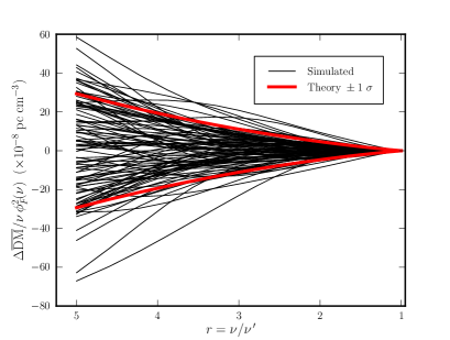
Figure 6.— Plot of $\Delta\overline{\rm DM}$ normalized by $\nu\phi_{F}^{2}(\nu)$ vs frequency ratio $r=\nu/{\nu^{\,\prime}}$ for 100 realizations (black lines). Also shown is $\pm F_{\beta}(r)$ scaled by the coefficient in Eq. 12 (red lines), which is the $\pm$ one standard deviation range of plotted values.

The difference in $\overline{\rm DM}$ between two frequencies $\nu$ and ${\nu^{\,\prime}}$ (measured at the same location ${{\bf x}}$, corresponding to the same epoch),

$$\Delta\overline{\rm DM}(\nu,{\nu^{\,\prime}},{{\bf x}})=\overline{\rm DM}({\nu^{\,\prime}},{{\bf x}})-\overline{\rm DM}(\nu,{{\bf x}}),$$ (7)

has an RMS difference,

$$\sigma_{\footnotesize\overline{\rm DM}}(\nu,{\nu^{\,\prime}})=\left\langle\left[\Delta\overline{\rm DM}(\nu,{\nu^{\,\prime}},\,{{\bf x}})\right]^{2}\right\rangle^{1/2}.$$ (8)

Electron-density wavenumber spectra with $\beta>2$ produce DM variations that are dominated by the largest scales. For these $\beta$, the relevant scales range from the smoothing length $\sigma_{X}\approx{D^{\prime}}{\theta_{d}}_{\nu}$ to the ‘outer scale’ of the spectrum that is likely determined by the sizes of structures and clouds in the ISM. The largest structures correspond to time variations in DM up to $10^{4}$ years or longer for parsec scales and characteristic velocities $\sim 100$ km s^-1. We are concerned with much shorter time scales for which the mean-square difference is an appropriate tool because large scale variations $\gg\sigma_{X}$ cancel out.

In Appendix B we derive the RMS DM difference using Gaussian smoothing functions and express the result in two forms, one that uses the scattering measure $SM=\int dz\ \rm C_{n}^{2}(z)$ and a second that uses the Fresnel phase evaluated at the higher frequency,

$$\sigma_{\footnotesize\overline{\rm DM}}(\nu,{\nu^{\,\prime}}) = F_{\beta}(\nu/{\nu^{\,\prime}})\times\left\{\begin{array}[]{ll}G_{\beta}Q_{\beta}\,r_{e}\ c^{\beta/2}\,D^{(\beta-2)/2}\nu^{-\beta/2}\,\rm SM&\quad\quad\quad\text{Scattering Measure}\\ \\ g_{\beta}\,q_{\beta}\left(\frac{\displaystyle\nu\phi_{F}^{2}(\nu)}{\displaystyle cr_{e}}\right)&\quad\quad\quad\text{Fresnel Phase}.\end{array}\right.$$ (12)

The dimensionless quantities $Q_{\beta},q_{\beta}$ depend only on the wavenumber spectrum while the dimensionless quantities $G_{\beta},g_{\beta}$ depend on the LOS distribution of $\rm C_{n}^{2}$ (thin screen vs. statistically uniform medium, etc.) as well as on the spectrum. Values for Kolmogorov media are given in Table 1. All of the relative frequency dependence is contained in the function $F_{\beta}(r)$,

$$F_{\beta}(r)=\left\{2^{(4-\beta)/2}\left[1+r^{2\beta/(\beta-2)}\right]^{(\beta-2)/2}-r^{\beta}-1\right\}^{1/2},$$ (13)

where $r\equiv\nu/{\nu^{\,\prime}}$. This vanishes for $r=1$, as expected and increases monotonically with $r$ for $2<\beta<4$.

For a Kolmogorov spectrum,

$$\sigma_{\footnotesize\overline{\rm DM}}(\nu,{\nu^{\,\prime}}) = F_{11/3}(r)\times\left\{\begin{array}[]{ll}3.76\times 10^{-5}\,{\rm pc~{}cm^{-3}}\,G_{11/3}\,D^{5/6}\nu^{-11/6}\,\rm SM_{-3.5}&\quad\quad\quad\text{Scattering Measure}\\ \\ \,4.42\times 10^{-5}\,{\rm pc~{}cm^{-3}}\,g_{11/3}\,\displaystyle\left[\frac{\nu\phi_{F}^{2}(\nu)}{1000}\right]&\quad\quad\quad\text{Fresnel Phase}.\end{array}\right.$$ (17)

where SM is expressed in units of $10^{-3.5}~{}\rm kpc~{}m^{-20/3}$, the distance $D$ in kpc, and the frequency $\nu$ in GHz; $\phi_{F}(\nu)$ is in radians.

The LOS is characterized by either SM or $\phi_{F}$, which can be estimated from the scintillation bandwidth $\Delta\nu_{d}$ and time scale $\Delta t_{\rm ISS}$. These are defined respectively as the half-width at half-maximum of the intensity correlation function vs. frequency difference and as the half-width at $1/e$ of the intensity correlation function vs. time lag. For a thin screen,

$$\rm SM_{-3.5}=0.74\,\nu^{11/3}\left(\Delta\nu_{d}D\right)^{-5/6}\left[(D_{s}/D)(1-D_{s}/D)\right]^{-5/6}$$ (18)

while for a statistically homogenous medium with constant $\rm C_{n}^{2}$,

$$\rm SM_{-3.5}=2.26\,\nu^{11/3}\left(\Delta\nu_{d}D\right)^{-5/6}.$$ (19)

To get $\phi_{F}$ we use the relationship between the pulse broadening time $\tau_{d}$ and the scintillation bandwidth, $\tau_{d}=C_{1}/2\pi\Delta\nu_{d}$, where $C_{1}$ is a constant of order unity (Cordes & Rickett, 1998; Lambert & Rickett, 1999),

$$\phi_{F}(\nu)=\sqrt{2}\left[\frac{C_{1}}{(D/D_{s})(1-D_{s}/D)}\right]^{(\beta-2)/4}\left(\frac{\nu}{\Delta\nu_{d}}\right)^{(\beta-2)/4}\approx 9.6~{}{\rm rad}\left(\frac{\nu/\Delta\nu_{d}}{100}\right)^{5/12},$$ (20)

where the quantity in square brackets $\sim{\cal O}(1)$ and the approximate expression is for a Kolmogorov spectrum. A ratio $\nu/\Delta\nu_{d}\sim 100$ is of order the value for nearby millisecond pulsars at $\nu=1$ GHz. A similar expression can be written in terms of the diffractive scintillation time scale $\Delta t_{\rm ISS}$ and the effective velocity $V_{\rm eff}$ by which the line of sight changes with time,

$$\phi_{F}(\nu)\approx 8~{}{\rm rad}\left(\sqrt{\nu}\,V_{\rm eff,100}\Delta t_{\rm ISS,1000}\right)^{-5/6},$$ (21)

with $V_{\rm eff}=100V_{\rm eff,100}$ km s^-1, and $\Delta t_{\rm ISS}=10^{3}\Delta t_{\rm ISS,1000}$ s. A relation between scattering measure and $\phi_{F}$ is given in Eq. A9.

Figure 6 shows $\Delta\overline{\rm DM}$ plotted against frequency ratio $r=\nu/{\nu^{\,\prime}}$ (black lines) based on simulations of phase screens with $\phi_{F}=30$ rad at 1 GHz. We also show the predicted RMS $\sigma_{\footnotesize\overline{\rm DM}}(\nu,{\nu^{\,\prime}})$ (red lines) indicating statistical consistency between the theoretical and simulation results. Individual realizations show a tendency for $\Delta\overline{\rm DM}$ to be dominated by a linear dependence on $r-1$, though there are counterexamples that show a significant quadratic dependence. In Section 3 we utilize this approximate linearity as a basis for possible mitigation of the effect in timing data.

3. Implications for Timing Accuracy

There are many complications to the estimation of arrival times. Recent work has addressed the removal of time-variable DMs (e.g. Pennucci et al., 2014; Lee et al., 2014; Liu et al., 2014) but no work to our knowledge has aimed at mitigating the frequency dependence. Other chromatic ISM effects include delays from diffraction and refraction that have been discussed elsewhere (e.g. Foster & Cordes, 1990; Rickett, 1990; Cordes & Shannon, 2010). Also important is the evolution with frequency of the intrinsic shape of a pulsar’s pulse (e.g. Craft & Comella, 1968; Craft, 1970; Ahuja et al., 2007; Hassall et al., 2012; Pennucci et al., 2014; Liu et al., 2014), which produces a systematic TOA error vs. frequency that is partially covariant with DM variations but is assumed to be independent of epoch. Since these and other effects are largely independent, their variances add and therefore can be discussed separately from the frequency-dependent effect analyzed here.

We consider multiple frequency measurements at a fixed epoch, so we drop any explicit time dependence from $\overline{\rm DM}$. A simple model for the TOA at frequency $\nu$ includes dispersive delays and measurement errors as perturbations of the ‘true’ TOA, $t_{\infty}$,

$$t_{\nu}=t_{\infty}+\frac{K\overline{\rm DM}(\nu)}{\nu^{2}}+\epsilon_{\nu}.$$ (22)

The quantity $\epsilon_{\nu}$ is an additive, frequency-dependent error that is uncorrelated between different frequencies for radiometer-noise but is highly correlated for intrinsic pulse jitter, at least over modest frequency separations.

3.1. Dual Frequency Measurements

An observing strategy exploits the lever-arm provided by widely-spaced frequencies to obtain a high-precision estimate for DM, which then is used to estimate a DM-compensated arrival time, $t_{\infty}$. Here we derive the resulting errors in DM and $t_{\infty}$.

Consider two arrival times $t_{\nu},t_{\nu^{\,\prime}}$ measured at frequencies $\nu$ and ${\nu^{\,\prime}}<\nu$ at the same epoch. The usual operational practice is to estimate DM (denoted by the caret) by inverting Eq. 22 under the assumption that DM is frequency independent,

$$\widehat{\rm DM}=\frac{t_{\nu^{\,\prime}}-t_{\nu}}{K({\nu^{\,\prime}}^{-2}-\nu^{-2})}.$$ (23)

The dispersion delay is then removed from the measured TOA $t_{\nu}$ to estimate the infinite-frequency TOA,

$$\widehat{t}_{\infty}=t_{\nu}-\frac{K\widehat{\rm DM}}{\nu^{2}}=t_{\infty}+\frac{K[\overline{\rm DM}(\nu)-\widehat{\rm DM}]}{\nu^{2}}+\epsilon_{\nu}.$$ (24)

For a frequency ratio $r=\nu/{\nu^{\,\prime}}$, the difference between the estimated and true $\overline{\rm DM}(\nu)$ is

$$\overline{\rm DM}(\nu)-\widehat{\rm DM}=\left(\frac{r^{2}}{r^{2}-1}\right)\left[\overline{\rm DM}(\nu)-\overline{\rm DM}({\nu^{\,\prime}})\right]+\frac{\nu^{2}\left(\epsilon_{\nu}-\epsilon_{\nu^{\,\prime}}\right)}{K}.$$ (25)

and the resulting error in the infinite-frequency TOA is

$$\delta t_{\infty}\equiv t_{\infty}-\widehat{t}_{\infty}=\frac{K}{\nu^{2}}\left(\frac{r^{2}}{r^{2}-1}\right)\Delta\overline{\rm DM}(\nu,{\nu^{\,\prime}})+\left(\frac{\epsilon_{\nu^{\,\prime}}-r^{2}\epsilon_{\nu}}{r^{2}-1}\right).$$ (26)

The estimator $\widehat{t}_{\infty}$ is unbiased if the DM variations and the errors $\epsilon_{\nu}$ have zero mean values over an ensemble. The contribution to $\delta t_{\infty}$ from the measurement error $\epsilon_{\nu}$ at the higher frequency is enhanced by a factor $r^{2}$. This means that the error at the lower frequency $\epsilon_{\nu^{\,\prime}}$ can be larger than the high-frequency error by a factor equal to a modest fraction of $r^{2}$ and not unduly affect the precision of $\widehat{t}_{\infty}$.

The combined RMS timing error $\sigma_{\widehat{t}_{\infty}}$ is the quadratic sum of the individual RMS errors,

$$\sigma_{\widehat{t}_{\infty}}=\left(\sigma_{t_{\infty},\delta\overline{\rm DM}}^{2}+\sigma_{t_{\infty},\epsilon}^{2}\right)^{1/2}.$$ (27)

3.1.1 TOA Error from Frequency-dependent DMs

The RMS DM difference $\sigma_{\overline{\rm DM}(\nu,{\nu^{\,\prime}})}$ defined in Eq. 12-13 implies an RMS error in TOA,

$$\sigma_{t_{\infty},\delta\overline{\rm DM}}=\frac{r^{2}}{|r^{2}-1|}\frac{K\sigma_{\overline{\rm DM}(\nu,{\nu^{\,\prime}})}}{\nu^{2}} = E_{\beta}(r)\times\left\{\begin{array}[]{ll}\displaystyle(2\pi)^{-1}G_{\beta}Q_{\beta}\,r_{e}^{2}\ c^{(\beta+2)/2}\,D^{(\beta-2)/2}\nu^{-(\beta+4)/2}\,\rm SM,&\quad\text{Scattering Measure}\\ \\ g_{\beta}\,q_{\beta}\left[\dfrac{\displaystyle\phi_{F}^{2}(\nu)}{\displaystyle 2\pi\nu}\right],&\quad\text{Fresnel Phase},\end{array}\right.$$ (31)

where the $r$-dependent factors have been combined into a timing-error function valid for $2<\beta<4$ (see Figure 13),

$$E_{\beta}(r)=\dfrac{r^{2}F_{\beta}(r)}{|r^{2}-1|}.$$ (32)

For a Kolmorovov spectrum, the RMS timing error is

$$\sigma_{t_{\infty},\delta\overline{\rm DM}} = E_{11/3}(r)\times\left\{\begin{array}[]{ll}156\,{\rm ns}\ G_{11/3}\,D^{5/6}\nu^{-23/6}\,\rm SM_{-3.5}&\quad\quad\quad\text{Scattering Measure}\\ \\ 184\,{\rm ns}\ g_{11/3}\,q_{11/3}\,\left[\displaystyle\dfrac{\nu^{-1}\phi_{F}^{2}(\nu)}{1000}\right]&\quad\quad\quad\text{Fresnel Phase}.\end{array}\right.$$ (36)

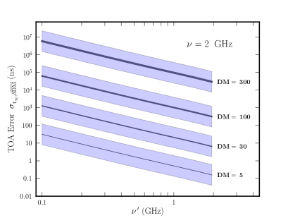
Figure 7.— RMS error in the DM-corrected TOA $t_{\infty}$ vs. frequency for a fixed upper frequency of 2 GHz and four values of average DM, as labeled. The curves for different DMs were calculated using the pulse-broadening time $\tau_{d}$ from the scaling law in Eq. 7 of Bhat et al. (2004) to obtain $\phi_{F}(\nu)$ using Eq. 20 and then evaluating Eq. 31 for different $r=\nu/{\nu^{\,\prime}}$. The spread in values demarked by the shaded regions results from the variation about the empirical mean relation between $\log_{10}\tau_{d}$ and $\log_{10}\rm DM$. While we show curves extending down to 0.1 GHz, pulse broadening will likely dominate the timing precision and will render some pulsars undetectable at lower frequencies.

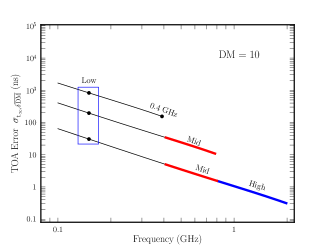
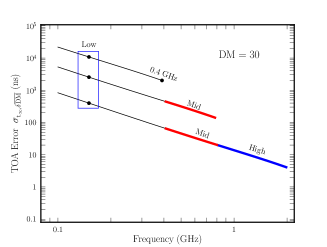
Figure 8.— RMS $t_{\infty}$ vs. frequency ${\nu^{\,\prime}}$ for dual-frequency observations for pulsars with $DM=10$ pc cm^-3 (left) and $DM=30$ pc cm^-3 (right). For each curve the rightmost frequency is the highest frequency of the pair and the curve gives $\sigma_{t_{\infty}}(\nu,{\nu^{\,\prime}})$. Lower $\nu$ have higher $\sigma_{t_{\infty}}(\nu,{\nu^{\,\prime}})$. Low, mid, and high-frequency bands are indicated.

Figure 7 shows $\sigma_{t_{\infty},\delta\overline{\rm DM}({\nu^{\,\prime}},\nu)}$ vs ${\nu^{\,\prime}}$ for $\nu=2$ GHz for four values of average DM. We calculated these curves by estimating the Fresnel phase at the reference frequency $\nu=2$ GHz using Eq. 20 and then expressing the scintillation bandwidth at the highest frequency $\nu$ in terms of the pulse broadening time using $\Delta\nu_{d}=C_{1}/2\pi\tau_{d}$. We get $\tau_{d}$ from the empirical relation $\log_{10}\tau_{d}(\mu s)=-3.46+0.154x+1.07x^{2}-[2\beta/(\beta-2)]\log_{10}\nu$ for $\nu$ in GHz (e.g. Bhat et al., 2004). The variation about this mean relation is $0.7$ in $\log_{10}\tau_{d}(\mu s)$. We use $\beta=11/3$ though Bhat et al. find a best-fit value that is slightly greater. The curves in the figure may therefore underestimate the timing error because we use $\nu=2$ GHz. The figure demonstrates the strong dependence of the TOA error on chromatic DMs because $\tau_{d}$ and thus $\phi_{F}$ increase nonlinearly with DM and the TOA error scales as the square of $\phi_{F}$.

Figure 8 complements Figure 7 by showing the TOA error for observations that involve different frequency ranges and for two different but rather low values of DM (10 and 30 pc cm^-3). Each curve in the figure corresponds to two-frequency observations where the higher frequency $\nu$ is the right-most frequency (2, 0.8, and 0.4 GHz) and the lower frequency ${\nu^{\,\prime}}$ is the horizontal axis. Obtaining TOAs with $<0.1~{}\mu s$ precision clearly requires a high frequency of no less than 0.8 GHz for low-DM pulsars. The curves presented here and in Figure 7 demonstrate that low frequency telescopes such as LOFAR need to be coupled with higher-frequency telescopes operating at $\mathrel{\hbox{\hbox to0.0pt{\hbox{\lower 4.0pt\hbox{$\sim$}}\hss}\hbox{$>$}}}2$ GHz to provide TOA errors $\mathrel{\hbox{\hbox to0.0pt{\hbox{\lower 4.0pt\hbox{$\sim$}}\hss}\hbox{$<$}}}0.1~{}\mu s$ from chromatic DMs. Note however, that the total DM-corrected timing error also involves radiometer noise and pulse jitter, which favor wide frequency spans that are discussed next.

3.1.2 Measurement Errors from Radiometer Noise, Pulse Jitter, and Diffractive Scintillations

To treat any kind of measurement error, we use a correlation function (normalized to unit maximum) $\rho_{\nu{\nu^{\,\prime}}}=\langle\epsilon_{\nu}\epsilon_{{\nu^{\,\prime}}}\rangle/\sigma_{\nu}\sigma_{\nu^{\,\prime}}$ between the errors at two frequencies. The RMS of the second term in Eq. 26 is then

$$\sigma_{t_{\infty},\epsilon} = \frac{\left[r^{4}\sigma_{\nu}^{2}+\sigma_{\nu^{\,\prime}}^{2}-2r^{2}\sigma_{\nu}\sigma_{\nu^{\,\prime}}\rho_{\nu{\nu^{\,\prime}}}\right]^{1/2}}{|r^{2}-1|}.$$ (37)

Radiometer noise ($\epsilon=$ rn) is uncorrelated between TOAs obtained using non-overlapping bandpasses, so $\rho_{\nu{\nu^{\,\prime}}}=0$ and

$$\sigma_{\widehat{t}_{\infty},\rm rn}=\dfrac{\sqrt{r^{4}\sigma_{\nu}^{2}+\sigma_{\nu^{\,\prime}}^{2}}}{|r^{2}-1|}.$$ (38)

In our analysis we consider wide frequency ranges with logarithmic spacings of frequencies and assume that bandwidths are proportional to frequency. This naturally leads to a power-law scaling of the TOA error from radiometer noise,

$$\frac{\sigma_{\rm rn,{\nu^{\,\prime}}}}{\sigma_{\rm rn,\nu}} = \left(\frac{{\nu^{\,\prime}}}{\nu}\right)^{x_{\rm rn}}\equiv r^{-x_{\rm rn}}.$$ (39)

We then rewrite Eq. 38 as

$$\sigma_{\widehat{t}_{\infty},\rm rn}=\dfrac{\sigma_{rn,\nu}\left(r^{4}+r^{-x_{\rm rn}}\right)^{1/2}}{|r^{2}-1|}.$$ (40)

Individual pulses show phase and amplitude jitter ($\epsilon=$ j) that cause small shape changes in the averages of large numbers of pulses used to calculate TOAs. The resulting TOA error is correlated between frequencies, sometimes highly so. If perfectly correlated ($\rho_{\nu{\nu^{\,\prime}}}=1$) and identical, jitter produces no error in $\widehat{\rm DM}$ because the TOAs move in tandem at the two frequencies (c.f. Eq. 25). The resulting TOA error from jitter is then simply $\sigma_{j}$. However, single pulses and average profiles evolve slowly with frequency, yielding random and systematic TOA errors, respectively. Generally the jitter correlation will be less than 100%, yielding a larger contribution to the TOA error than from perfectly correlated jitter. However, the frequency separation over which single pulses decorrelate is large for the few cases that have been studied. These include the Crab pulsar (Sallmen et al., 1999) which decorrelates over about 0.7 GHz and the millisecond pulsar J0437-4715, which decorrelates over a 2-GHz bandwidth (Shannon et al., 2014). For the brightest pulsars, the TOA errors from jitter and radiometer noise are comparable (Shannon & Cordes, 2012; Dolch et al., 2014; Shannon et al., 2014) so when pulse jitter is not completely correlated, mis-estimation of DM is comparable to that from radiometer noise.

We adopt a power-law scaling analogous to that for radiometer noise,

$$\frac{\sigma_{\rm j,{\nu^{\,\prime}}}}{\sigma_{\rm j,\nu}} = \left(\frac{{\nu^{\,\prime}}}{\nu}\right)^{x_{\rm j}}\equiv r^{-x_{\rm j}}.$$ (41)

The resulting expression for the jitter-induced timing error for perfect correlation between frequencies ($\rho_{\nu{\nu^{\,\prime}}}=1$) is

$$\sigma_{\widehat{t}_{\infty},\rm j}=\frac{\sigma_{j,\nu}|r^{2}-r^{-x_{\rm j}}|}{|r^{2}-1|}.$$ (42)

Diffractive scintillations (DISS) have correlation times and bandwidths that range, respectively, from minutes to hours and $\sim 100$ kHz to 100s of MHz at 1 GHz for currently timed millisecond pulsars (MSPs), which tend to have low DMs $\mathrel{\hbox{\hbox to0.0pt{\hbox{\lower 4.0pt\hbox{$\sim$}}\hss}\hbox{$<$}}}30$ pc cm^-3. DISS causes TOA errors because the associated pulse broadening function — the scattering impulse response of the ISM that is convolved with a pulsar’s pulse — is stochastic on the DISS correlation time scale. The RMS TOA error at an individual frequency is much smaller than those from radiometer noise and jitter for nearby MSPs but can be comparable for more distant ones (Lam et. al, in preparation).

Scintillations of a low-DM MSP will yield a non-zero correlation $\rho_{\nu{\nu^{\,\prime}}}$ for observations made nearly simultaneously (e.g. within less than one hour) and with frequencies separated by no more than a correlation bandwidth. Most current timing observations are made with large-enough bandwidths or frequency separations and many observations are made non-simultaneously, in which case $\rho_{\nu{\nu^{\,\prime}}}=0$.

3.1.3 Systematic Errors from Profile Evolution

Profile evolution ($\epsilon=$ ’pe’) is known to introduce systematic errors in TOAs because the average profile changes smoothly with frequency. They can also be described using Eq. 26. However, unlike the random errors in the previous section, profile evolution can be mitigated by exploiting its apparent epoch independence (e.g. Pennucci et al., 2014) and thus differs from the chromatic DM effect that varies with epoch.

3.1.4 Assessment of Two-Frequency Timing

It is often assumed that wider frequency separations yield more precise dispersion measures and arrival times. We assess this approach by considering the timing error from frequency-dependent DMs combined with measurement errors. The results indicate that there can be diminishing if not worsening returns once the frequency ratio becomes larger than about a factor of two and if no mitigation procedure is used. We note that the same affliction arises from evolution of pulse shapes with frequency, as mentioned earlier.

In Figure 9 we plot $\sigma_{\widehat{t}_{\infty}}$ from Eq. 27 and the individual contributions to it from frequency-dependent DMs, radiometer noise, and pulse jitter using Eq. 36, 38, and 42, respectively. The specific case shown uses RMS values of 100 ns for both the noise and jitter contributions that are frequency independent ($x_{\rm rn}=x_{\rm j}=0$). The DM error was calculated for a scattering measure $\log_{10}\rm SM=-3.5$, a value that is typical of pulsars within $1$ kpc of Earth. The figure shows basic features that are generic. Rather than decreasing monotonically or remaining flat, as expected from radiometer noise or pulse jitter alone, the TOA error reaches a minimum at $r\mathrel{\hbox{\hbox to0.0pt{\hbox{\lower 4.0pt\hbox{$\sim$}}\hss}\hbox{$<$}}}2$ and then rises as the frequency-dependent DM contribution begins to dominate. Other cases with different mixtures of radiometer noise and jitter and different indices $x_{\rm rn}$ and $x_{\rm j}\neq 0$ are qualitatively similar.

Other examples are shown in Figure 9, including those with very small (10 ns) contributions from noise and jitter. While some cases — those with large noise or jitter contributions — do not show a minimum in $r$, all show much larger asymptotic TOA errors than expected from radiometer noise and jitter alone. This implies that increases in bandwidth with wideband systems will provide diminishing returns unless the frequency-dependent DM can be mitigated, as discussed below.

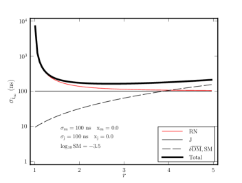
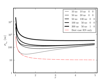
Figure 9.— (Left) RMS error of $t_{\infty}$ for two-frequency measurements as a function of $r={\nu^{\,\prime}}/\nu$ for a fiducial (highest) frequency of 1 GHz. Individual contributions are shown from radiometer noise, pulse jitter, and frequency-dependent DMs along with the total (heavy black line). For this case we assume that the noise and jitter errors are both $100$ ns and do not depend on frequency. Results are not dramatically different for cases where they are frequency dependent. (Right) Total TOA error vs $r$ for six different mixtures of timing errors from radiometer noise, jitter, and frequency dependent DMs. The legend gives the TOA errors from RMS noise $\sigma_{\rm t,rn}$, from RMS jitter, and their frequency scaling indices, $x_{\rm rn}$ and $x_{\rm j}$ respectively. The dashed curve gives the TOA error if only radiometer noise with 10 ns RMS contributed to timing errors.

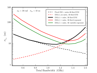
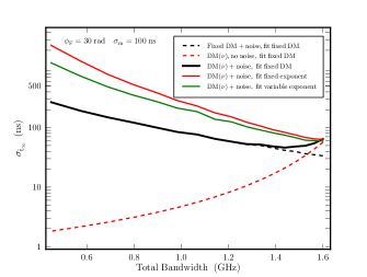
Figure 10.— RMS TOA error from wideband fitting for DM and $t_{\infty}$ over a continuous frequency range from 0.4 to 2 GHz. The phase screen has a Fresnel RMS phase of $30$ rad and the RMS radiometer noise is an optimistic 10 ns (left) and 100 ns (right) that is assumed to be constant in frequency. A total of 2000 phase-screen realizations was used. The cases shown include (1) Fixed true DM is fixed and a timing model that includes only $t_{\infty}$ and a $\nu^{-2}$ term; (2) Variable DM without noise added and a fit for fixed DM; (3) Variable DM with noise and a fit for fixed DM; (4) As with (3) but with a fit that also includes a $\nu^{-X}$ term with fixed $X=3$; and (5) As with (4) but where the exponent $X$ is also fitted for.

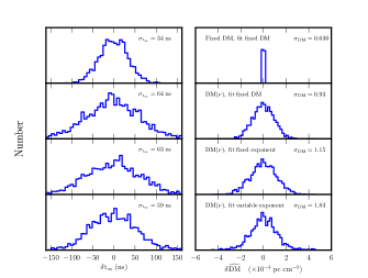
Figure 11.— Results from wideband fitting for DM and $t_{\infty}$ over a continuous frequency range from 0.4 to 2 GHz. The phase screen has a Fresnel RMS phase of $30$ rad and the RMS radiometer noise is constant in frequency: 10 ns (left set of panels) and 100 ns (right). Left column: histograms of the error in $t_{\infty}$ based on 2000 realizations of a phase screen. RMS values for $t_{\infty}$ are given in each panel. Right column: histograms of the difference in DM from the value at the highest frequency. RMS values for $\delta\overline{\rm DM}$ are given in units of $10^{-4}$ pc cm^-3. First row: the true DM is fixed and the timing model includes only a $\nu^{-2}$ term; Second row: same as the first case except that DM varies with frequency; Third row: DM varies with frequency and the timing model includes both a $\nu^{-2}$ and a $\nu^{-X}$ term with $X=3$ (fixed); and Fourth row: same as previous except that the exponent is also fitted for.

3.2. Wideband Timing Measurements

Digital backend systems developed recently for pulsar observations have much larger frequency ranges (1.8:1) than previous systems and provide the opportunity to estimate TOAs over a continuous range of frequencies rather than using two narrowband frequencies with a wide separation (e.g. Pennucci et al., 2014). Even wider bandwidth systems are contemplated with 4:1 (or larger) frequency ranges.

We analyze wideband systems with arbitrary total bandwidths by using standard least-squares fitting methods to fit data without and with frequency-dependent DMs. We let the data vector ${\bf D}$ comprise a set of TOAs $\{t_{\nu_{k}},\,k=1,\ldots,N_{\nu}\}$ and their measurement errors $\sigma_{\nu_{k}}$ for $N_{\nu}$ separate frequencies measured at the same epoch. For simplicity, we consider only radiometer noise in the wideband analysis, corresonding to a diagonal covariance matrix, ${\bf C}={\rm diagonal}\left\{\sigma_{\nu_{k}}^{2}\right\}$. For a design matrix ${\bf X}$ and a linear model ${\bf D}={\bf X}{\mbox{\boldmath$\theta$}}+{\mbox{\boldmath$\epsilon$}}$, the solution vector is ${\mbox{\boldmath$\theta$}}=\left({\bf X}^{\dagger}{\bf C}^{-1}{\bf X}\right)^{-1}{\bf X}^{\dagger}{\bf C}^{-1}{\bf D}$ and the covariance matrix for the parameters is ${\bf P_{{\mbox{\boldmath$\theta$}}}}=\left({\bf X}^{\dagger}{\bf C}^{-1}{\bf X}\right)^{-1}$.

With respect to the timing model of Eq. 22, we consider four alternatives:

1. First is where the frequency-dependent DM is negligible so DM is constant in frequency and the only errors are from radiometer noise. This would be the case for a very low-DM pulsar or measurements at high frequencies $\nu\gg 1$ GHz. The data are fitted with a parameter vector ${\mbox{\boldmath$\theta$}}={\rm col}\left(t_{\infty},K\rm DM\right)$ and corresponding design matrix ${\bf X}={\rm matrix}(1\,\,\,\nu_{i}^{-2}),i=1,\ldots,N_{\nu}$. The solution vector is unbiased.

2. The second case is where the frequency dependence of DM is significant but the data are still fitted with a constant DM model. The results are generally biased.

3. The third case is motivated by recognizing in Figure 6 that DM differences $\Delta\overline{\rm DM}({\nu^{\,\prime}},\nu)$ have a tendency to appear roughly (but not exactly) linear in $r-1$; this suggests that a term in the fitting function scaling as $\nu^{-3}$ will absorb much of the effect and improve the estimate for $t_{\infty}$.

4. The fourth case is the same as the third except the fitting function includes a $\nu^{-x}$ term where $x$ is also fitted for as a (nonlinear) parameter instead of fixing it at $x=3$.

Example results in Figure 10 show the TOA error plotted against total bandwidth for $\nu=2$ GHz (the highest frequency) with a total of 20 separate frequencies used. DM variations are for a phase screen with $\phi_{F}=30$ rad at $\nu=1$ GHz. In the left-hand panel we have used an optimistic 10 ns for the radiometer noise at the fiducial frequency of 1 GHz while in the right-hand panel we have used 100 ns. We do not include pulse jitter in these examples because results shown previously indicate that it is secondary. Curves are shown for the four cases described above along with a fifth case that is an extreme version of case 2 where the noise is assumed negligible. The results are similar to those obtained in the two-frequency case. Namely, for the 10-ns noise case, increases in bandwidth yield improvements until the bandwidth is about 1 GHz and then the results degrade if there is no explicit fitting for the frequency-dependent DM. With such fitting (cases 3 and 4 above), the bandwidth can be increased another 20 to 40% before the timing errors degrade. For the larger 100-ns noise in the right-hand panel, TOA errors are dominated by radiometer noise except for the largest bandwidths for which there is an increase in timing error.

Figure 11 shows additional information on fitting results using histograms of the errors in $t_{\infty}$ and $\rm DM$. The two cases shown are for the same fits and data model used to produce Figure 10. The top rows show fitting results when the DM is constant in frequency and the sole source of fitting error is the additive noise. Other rows show the results for the different methods outlined above to deal with the frequency dependence of DM. Overall, Figures 10 and 11 show that allowance for the frequency dependence can reduce the timing error but cannot achieve the same results as for a constant DM.

3.3. Other Mitigation Methods

So far we have discussed estimation and removal of dispersion using data obtained at a single epoch. To date, most methods used by groups aiming to detect gravitational waves have used multiple epochs to estimate DM at the epoch of any particular arrival time.While using multiple epochs can be deleterious (e.g. Lam et al., 2015), they can be implemented with algorithms that take into account the correlation times of DM variations that result from ray-path averaging. These times can be days to months or longer depending on the frequency and ISM along the line of sight.

It is beyond the scope of this paper to develop a multi-epoch approach. However, we can illustrate a two-frequency approach that smooths the DM time series at a high frequency to match the characteristic time scale of the low-frequency DM variations. Figure 12, shows DM variations at 0.2 and 1.5 GHz from a simulation for a phase screen with $\phi_{F}=30$ rad at 1 GHz. In the top panel, the high-frequency time series has been optimally smoothed using a Gaussian smoothing function that minimizes the mean-square difference with the low-frequency time series. The bottom panel of the figures shows the smoothed and unsmoothed DM difference between the two frequencies. While the differences have been reduced by smoothing the high-frequency DM, they are not negligible because one-dimensional smoothing cannot model the two-dimensional smoothing that occurs in the ISM from scattering. Nonetheless, this approach can be used as a mitigation procedure.

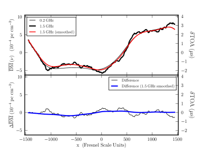
Figure 12.— Test of one-dimensional smoothing to estimate the two-dimensional averaging from scattering using DM variations for a scattering screen with $\phi_{F}=30$ rad. The left-hand axis label is DM units and the right-hand axis is in time-delay units. (Top): $\overline{\rm DM}(\nu)$ vs. $x$ for two widely space frequencies, 0.2 and 1.5 GHz. Also shown (red line) is the smoothed 1.5 GHz variation that best matches the 0.2 GHz curve using a Gaussian smoothing function. (Bottom): DM differences without and with smoothing of the high frequency variation.

3.4. Weak Scattering

Our analysis applies to the strong scattering regime where $\phi_{F}>1$. Nearby pulsars observed at higher frequencies may be in weak scattering with $\phi_{F}<1$. In this regime, the scattered pulsar image consists of the very compact image of the unscattered pulsar that contains a fraction $\sim 1-\phi_{F}^{2}$ of the total flux combined with a scattered image with the remaining fraction. For small $\phi_{F}$, the cross-sectional area that is averaged is very small and the DM will be nearly achromatic. This would be another advantage of using high frequencies — defined as those above the transition frequency to weak scattering. The transition frequency is derived by requiring $\phi_{F}<1$ rad and using Eq. A9 to get $\nu_{\rm trans}\approx 8~{}{\rm GHz}~{}\rm SM_{-3.5}^{6/17}D^{5/17}$. For some pulsars, the transition frequency is $\mathrel{\hbox{\hbox to0.0pt{\hbox{\lower 4.0pt\hbox{$\sim$}}\hss}\hbox{$<$}}}1$ GHz (e.g. Rickett et al., 2000). However, precise DM estimates require multiple-frequency (or wideband) observations that almost always will use lower frequencies that are in the strong-scattering regime. We therefore see no way to avoid the chromatic aspect of DMs in precision timing.

4. Summary and Conclusions

We have shown that dispersion measures are chromatic because microstructure in the interstellar electron density causes multipath propagation that is strongly frequency dependent. We have characterized the effect in terms of the average over ray paths, $\overline{\rm DM}$, using an averaging kernel that is frequency dependent. Results were given for media having a power-law electron-density wavenumber spectrum and for arbitrary variations in amplitude of the spectrum along the line of sight. We verified our analytical results with simulations of phase screens with a Kolmogorov spectrum. Differences in $\overline{\rm DM}$ between two frequencies scale as $\phi_{F}^{2}/\lambda r_{e}\propto\rm SM$, where $\phi_{F}$ is the RMS phase across a Fresnel scale at the highest frequency used and $\rm SM$ is the scattering measure. Observations at frequencies $\mathrel{\hbox{\hbox to0.0pt{\hbox{\lower 4.0pt\hbox{$\sim$}}\hss}\hbox{$<$}}}1$ GHz will have $\phi_{F}\gg 1$ for most pulsars and $\phi_{F}\propto\nu^{-17/12}$. The specific variation of $\overline{\rm DM}$ with frequency will remain constant in time over a refraction time scale of hours to months (or longer) that is generally larger for larger-DM pulsars. The joint variation of $\overline{\rm DM}$ in time and frequency thus differs from that of intrinsic profile evolution, which appears to be epoch independent for millisecond pulsars. Longer period pulsars show state switching (nulling, mode changes, etc.) on a wide range of time scales, but the switching statistics appear to have stationary statistics.

As yet, there has been no direct detection of chromatic DMs. This is not surprising because there has been no detailed analysis prior to the present paper other than a brief discussion in Cordes & Shannon (2010), and its effects would be impossible to identify uniquely in dual-frequency TOA measurements typically employed. However, departures from the $\nu^{-2}$ dispersion delay appropriate for a tenuous, cold, unmagnetized plasma have been searched for and used to put limits on chromatic timing effects that scale differently than the standard $\nu^{-2}$ dispersion law (e.g. Hassall et al., 2012, and references therein). Such departures are complicated by profile evolution with frequency that is mitigated by identifying fiducial pulse phases that yield consistency with the cold-plasma law. Most of the objects analyzed this way (pulsars and fast radio bursts of apparent extragalactic origin) have much coarser timing precision than the MSPs used in pulsar timing arrays. The best prospects for detection are from a bright, high-DM pulsar that has minimal profile evolution over the frequency range needed to probe DM variations. Profile evolution may be disentangled from chromatic DMs by exploiting the lack of (or minimal) epoch dependence of profile evolution in comparison with variations in DM that have a characteristic correlation time for each frequency. It is conceivable that some of the frequency-dependent timing variations observed from the MSP J1909$-$3744 (e.g. Fig. 7 in Manchester et al., 2013) include the chromatic DM effect.

Chromatic DMs have a significant impact on pulsar timing applications where sub-microsecond timing accuracy is needed, such as detection of gravitational waves with pulsar-timing arrays and high-order general relativistic effects in binary pulsars. All pulsar timing applications depend on removing dispersion delays with high accuracy to estimate TOAs unaffected by propagation through the ISM, which we have called $t_{\infty}$. We have analyzed errors in $t_{\infty}$ resulting from methodologies that assume DMs are achromatic for two cases, one where TOAs are measured at pairs of widely separated frequencies and a second that uses continuous, wideband systems. Chromatic DMs introduce errors in $t_{\infty}$ that depend strongly on the pulsar’s mean DM and on the particular range of frequencies used. For nearby pulsars with $\rm DM\mathrel{\hbox{\hbox to0.0pt{\hbox{\lower 4.0pt\hbox{$\sim$}}\hss}\hbox{$<$}}}30$ pc cm^-3 and an octave frequency range with 1.5 GHz as the highest frequency, TOA errors solely from the chromatic part of DM are of order a few to hundreds of nanoseconds for observations extending down to 1 GHz or 0.2 GHz. Timing errors increase rapidly with increasing mean DM and timing residuals will be correlated on time scales related to those of refractive interstellar scintillations.

Timing errors from radiometer noise and pulse jitter combined with chromatic DMs show a broad minimum as a function of total frequency range (or bandwidth) that is of order an octave in frequency. This arises because TOAs improve monotonically with bandwidth as far as radiometer noise is concerned, but the opposite is true for chromatic DMs. The simplest prescription for optimizing TOA precision is to use an upper frequency that is as high as possible. The choice of upper frequency is strongly pulsar and telescope dependent.

Chromatic DMs also need to be considered in combination with other chromatic effects, including intrinsic pulse profile evolution with frequency and additional interstellar delays that result directly from scattering and refraction that have different frequency dependences than any of the DM effects. A comprehensive assessment of effects like that in Cordes & Shannon (2010) that includes the chromatic DM effect is deferred to a separate paper. Even though the timing errors from chromatic DMs are smaller than other effects, they nonetheless may inhibit improvements in timing accuracy that otherwise might be obtainable. It is therefore important to confirm that chromatic DMs are present in timing data at predicted levels and develop ways to mitigate them, if possible. If not, they need to be part of the noise model for timing analysis and incorporated into the covariance matrix used in model fitting.

In a separate article we will assess the role of chromatic DMs for all objects currently being observed in pulsar timing array campaigns to detect gravitational waves and we will also assess different methodologies for using existing and future telescopes. We will also identify particular pulsars that are good candidates for direct detection of DM chromaticity.

Appendix A Phase Structure Function and Scattering Angle

The phase structure function is the integral from a point source to an observer at distance $D$ from a point source,

$$D_{\phi}({\mbox{\boldmath$b$}})=\left\langle\left[\phi({{\bf x}})-\phi({{\bf x}}+{\mbox{\boldmath$b$}})\right]^{2}\right\rangle=4\pi(r_{e}\lambda)^{2}\int_{0}^{D}dz\,\int d{\bf q}_{\perp}\,P_{\delta n_{e}}({\bf q}_{\perp},z)\left(1-e^{i\displaystyle{\bf q}_{\perp}\cdot{\mbox{\boldmath$b$}}z/D}\right)$$ (A1)

where $b$ is a spatial offset and ${\bf q}_{\perp}$ a vector wavenumber transverse to the line of sight. This form applies to a wavenumber spectrum $P_{\delta n_{e}}$ whose extent in wavenumber is much narrower than $D^{-1}$, has a shape independent of $z$, and an amplitude that varies slowly with $z$. Normalization is so that the mean-square electron density is the integral of $P_{\delta n_{e}}$ over all wavenumbers, and $\int_{-\infty}^{\infty}\!dz\,e^{iq_{z}z}=2\pi\delta(q_{z})$.

Scattering measurements indicate various degrees of anisotropy of density fluctuations, but the isotropic case is easier to analyze. To treat the anisotropic case is tedious and does not add any further insights to the results obtained for the isotropic case. For isotropic irregularities only the magnitudes of $b$ and ${\bf q}_{\perp}$ matter, yielding

$$D_{\phi}(b)=8\pi^{2}(r_{e}\lambda)^{2}\int_{0}^{D}dz\,\int dq_{\perp}\,q_{\perp}P_{\delta n_{e}}(q_{\perp},z)[1-J_{0}(q_{\perp}bz/D)],$$ (A2)

where $J_{0}$ is the Bessel function of the first kind. We adopt a power-law wavenumber spectrum,

$$P_{\delta n_{e}}({q_{\perp}},z)=\rm C_{n}^{2}(z)q^{-\beta},\quad\quad q_{0}\leq q\leq q_{1},$$ (A3)

where $\rm C_{n}^{2}(z)$ varies slowly with $z$ on length scales much larger than the outer scale, $2\pi/q_{0}$. For $b\ll q_{1}^{-1}$ (i.e. $b$ smaller than the inner scale), the phase structure function is quadratic in $b$ while for $b\gg q_{0}^{-1}$ it asymptotes to twice the total variance of the phase. In the intermediate regime where $q_{1}^{-1}\ll b\ll q_{0}^{-1}$,

$$D_{\phi}(b)\approx f_{\beta}(\lambda r_{e})^{2}\rm SM_{\rm eff}\ b^{\beta-2},$$ (A4)

where (Cordes & Rickett 1998; Eq. B6)

$$f_{\beta}=\frac{8\pi^{2}}{(\beta-2)2^{\beta-2}}\frac{\Gamma(2-\beta/2)}{\Gamma(\beta/2)},$$ (A5)

where the effective scattering measure is the line-of-sight weighted integral of $\rm C_{n}^{2}$,

$$\rm SM_{\rm eff}=\int_{0}^{D}dz\,\rm C_{n}^{2}(z)\left(\frac{z}{D}\right)^{\beta-2}\equiv\rm SM\times\frac{\int dz\,\rm C_{n}^{2}(z)(z/D)^{\beta-2}}{\int dz\,\rm C_{n}^{2}(z)}\equiv\rm SM\left\langle(z/D)^{\beta-2}\right\rangle_{\rm C_{n}^{2}},$$ (A6)

where the angular brackets denote an average over the LOS using $\rm C_{n}^{2}(z)$ as a weighting function and the scattering measure is

$$\rm SM\equiv\int_{0}^{D}dz\,\rm C_{n}^{2}(z).$$ (A7)

For a screen, $\rm SM_{\rm eff}=(D_{s}/D)^{\beta-2}\ \rm SM$ and for a uniform medium with $\rm C_{n}^{2}=$ constant, $\rm SM_{\rm eff}=\rm SM/(\beta-1)$. A plane wave incident on a foreground scattering medium so that $D_{s}/D\to 1$ gives $\rm SM_{\rm eff}\equiv SM$ (e.g. for an extragalactic pulse incident on the Milky Way). Values for $\rm SM_{\rm eff}/SM$ are given in Table 1 for a Kolmogorov spectrum along with other parameters quantities.

Alternatively we can express the phase structure function in terms of the RMS phase $\phi_{F}$ across a Fresnel radius $r_{F}$ in the screen. We define the Fresnel scale using $r_{F}^{2}=[(\lambda D)/2\pi]D_{\rm eff}/D$ where for a thin screen $D_{\rm eff}=D_{s}{D^{\prime}}/D=D(D_{s}/D)(1-D_{s}/D)$. For a statistically uniform medium we assume $D_{\rm eff}=D/4$. Taking into account that a transverse scale $b$ at an observer’s position corresponds to a scale $zb/D$ at a position $z$ along the LOS, we have for a thin screen at $z=D_{s}$,

$$D_{\phi}(b)=\phi_{F}^{2}\left(\frac{D_{s}}{D}\right)^{\beta-2}\left(\frac{b}{r_{F}}\right)^{\beta-2}.$$ (A8)

From this and Eq. A7 we solve for $\rm SM$ in terms of $\phi_{F}$,

$$\rm SM=\frac{1}{f_{\beta}r_{F}^{\beta-2}}\frac{\phi_{F}^{2}}{(\lambda r_{e})^{2}}.$$ (A9)

In the following we assume the same relation holds generally though we have derived it from the thin-screen case.

The scattered image of a point source has longer tails than a Gaussian function for $\beta<4$ and an inner scale $2\pi/q_{1}$ much smaller than the Fresnel scale (e.g. Rickett, 1990). However it is convenient to characterize the main part of the image with an equivalent Gaussian whose visibility function has the same $1/e$ width. This defines the spatial scale $b_{e}$ using $D_{\phi}(b_{e})=2$,

$$b_{e}=\left[\frac{2}{f_{\beta}(\lambda r_{e})^{2}\rm SM_{\rm eff}}\right]^{1/(\beta-2)},$$ (A10)

from which the RMS angular size $\sigma_{\theta}$, the $1/e$ half width, and the full width at half maximum (FWHM) are calculated as

$$\sigma_{\theta}=\frac{\theta_{e}}{\sqrt{2}}=\frac{\theta_{\rm FWHM}}{2\sqrt{2\ln 2}}=\frac{\lambda}{\sqrt{2}\pi b_{e}}.$$ (A11)

The power-law spectrum yields an RMS angular size that we factor into a scattering size $\sigma_{\theta_{s}}$ and a geometry-dependent factor,

$$\sigma_{\theta}\equiv\sigma_{\theta_{s}}\left(\frac{\rm SM_{\rm eff}}{\rm SM}\right)^{1/(\beta-2)},\quad\quad\quad\sigma_{\theta_{s}}=\frac{1}{\pi}\left[\frac{\lambda^{\beta}f_{\beta}r_{e}^{2}\rm SM}{2^{\beta/2}}\right]^{1/(\beta-2)}.$$ (A12)

Appendix B Two-frequency Cross Correlation and Structure Function

We calculate the mean-square of the difference $\Delta\overline{\rm DM}(\nu,{\nu^{\,\prime}},{{\bf x}})=\overline{\rm DM}({\nu^{\,\prime}},{{\bf x}})-\overline{\rm DM}(\nu,{{\bf x}})$ defined in the main text to get the two-frequency structure function,

$$\sigma_{\footnotesize\overline{\rm DM}}^{2}(\nu,{\nu^{\,\prime}}) = \left\langle\left[\Delta\overline{\rm DM}(\nu,{\nu^{\,\prime}},\,{{\bf x}})\right]^{2}\right\rangle={C_{\delta\overline{\rm DM}}}(\nu,\nu)+{C_{\delta\overline{\rm DM}}}({\nu^{\,\prime}},{\nu^{\,\prime}})-2{C_{\delta\overline{\rm DM}}}({\nu^{\,\prime}},\nu)$$ (B1)

where the cross correlation of $\delta\overline{\rm DM}=\overline{\rm DM}-\left\langle\rm DM\right\rangle$ between two frequencies is

$$C_{\delta\overline{\rm DM}}(\nu,{\nu^{\,\prime}})=\left\langle\delta\overline{\rm DM}(\nu,{{\bf x}})\delta\overline{\rm DM}({\nu^{\,\prime}},{{\bf x}})\right\rangle=\iint\!d{{\bf x}^{\prime}}d{\bf x^{\prime\prime}}\iint\!dz^{\,\prime}dz^{\,\prime\prime}\,{A_{\nu}({{\bf x}^{\prime}},z^{\,\prime})}{A_{{\nu^{\,\prime}}}({\bf x^{\prime\prime}},z^{\,\prime\prime})}\langle\delta n_{e}({{\bf x}^{\prime}},z^{\,\prime})\delta n_{e}({\bf x^{\prime\prime}},z^{\,\prime\prime})\rangle.$$ (B2)

The $z$ integrals are from $0$ to $D$ and the ${{\bf x}}$ integrals are over an infinite plane. We define the cross-correlation function of the averaging function,

$$C_{A}({\delta{{\bf x}}},z,\nu,{\nu^{\,\prime}})=\int d{\overline{{{\bf x}}}}\,A_{{\nu^{\,\prime}}}({\overline{x}}-{\delta{{\bf x}}}/2,z)A_{\nu}({\overline{x}}-{\delta{{\bf x}}}/2,z),$$ (B3)

and assume that it changes slowly in $z$. By changing variables from ${{\bf x}^{\prime}},{\bf x^{\prime\prime}}$ to ${\overline{{{\bf x}}}}=({{\bf x}^{\prime}}+{\bf x^{\prime\prime}})/2$ and ${\delta{{\bf x}}}={{\bf x}^{\prime}}-{\bf x^{\prime\prime}}$ and from $z^{\,\prime},z^{\,\prime\prime}$ to ${z}=(z^{\,\prime}+z^{\,\prime\prime})/2$ and $\delta z=z^{\,\prime}-z^{\,\prime\prime}$, and using the hierarchy of scales assumed in Appendix A, the integration over $\delta z$ gives $2\pi\delta(q_{z})$ and we obtain

$$\sigma_{\footnotesize\overline{\rm DM}}^{2}(\nu,{\nu^{\,\prime}}) = \frac{1}{2}\int d{z}\!\!\int\!d\delta{{\bf x}}\,\int d\delta zD_{\delta n_{e}}(\delta{{\bf x}},\delta z;{z})\left[2C_{A}(\delta{{\bf x}},{z},\nu,{\nu^{\,\prime}})-C_{A}(\delta{{\bf x}},{z},\nu,\nu)-C_{A}(\delta{{\bf x}},{z},{\nu^{\,\prime}},{\nu^{\,\prime}})\right];$$ (B4)

$D_{\delta n_{e}}(\delta{{\bf x}},\delta z;{z})=\left\langle[\delta n_{e}({{\bf x}},z)-\delta n_{e}({{\bf x}}+\delta{{\bf x}},z+\delta z)]^{2}\right\rangle$ is the structure function for the electron density. For the power-law spectrum of Appendix A we have

$$\int d\delta{z}\,D_{\delta n_{e}}(\delta{{\bf x}},\delta z,{z})=f_{\beta}\rm C_{n}^{2}({z})\left(\delta x\right)^{\beta-2}.$$ (B5)

We now adopt the Gaussian smoothing function of Eq. 6 and employ the frequency scaling of $\sigma_{X}$, which is the same as that of the RMS scattering angle $\sigma_{\theta}\propto\nu^{-x_{\theta}}$ with $x_{\theta}=\beta/(\beta-2)$. By referencing frequency-dependent quantities to the higher frequency $\nu$ we get

$$\sigma_{\footnotesize\overline{\rm DM}}^{2}(\nu,{\nu^{\,\prime}})=\frac{(2\pi)^{2}\Gamma(2-\beta/2)}{\beta-2}F^{2}_{\beta}(\nu/{\nu^{\,\prime}})\int d{z}\,\rm C_{n}^{2}({z})\sigma_{X}^{\beta-2}({z},\nu)$$ (B6)

where the frequency-scaling function is

$$F_{\beta}(r)=\left\{2^{(4-\beta)/2}\left[1+r^{2\beta/(\beta-2)}\right]^{(\beta-2)/2}-r^{\beta}-1\right\}^{1/2}.$$ (B7)

Figure 13 shows $F_{\beta}(r)$ along with a related function $E_{\beta}(r)=r^{2}F_{\beta}(r)/(r^{2}-1)$ that is used in the main text to characterize time-of-arrival errors.

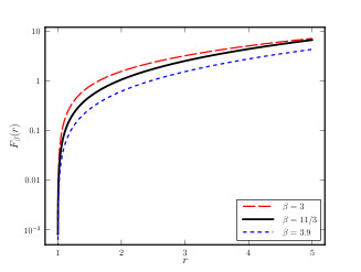
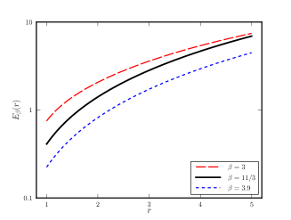
Figure 13.— (Left) The frequency scaling function $F_{\beta}(r)$ vs. $r=\nu/{\nu^{\,\prime}}$ for three values of $\beta$. (Right) The frequency scaling function $E_{\beta}(r)$ for the same three values of $\beta$.

To evaluate the integral in Eq. B6 we need expressions for how the transverse extent of the ray path bundle varies with $z$. We define

$$\sigma_{X}({z},\nu)=D\sigma_{\theta}(\nu)h(z/D)$$ (B8)

where $h(x)=1-x$ for a thin screen, $h(x)=x(1-x)$ for a statistically homogeneous medium, and $h(x)=1$ for a plane wave incident on the medium. We then define

$$H_{\beta}=\frac{\int d{z}\rm C_{n}^{2}({z})[h({z}/D)]^{\beta-2}}{\int d{z}\rm C_{n}^{2}({z})}\equiv\left\langle[h(z/D)]^{\beta-2}\right\rangle_{\rm C_{n}^{2}}.$$ (B9)

For a thin screen, $H_{\beta}=({D^{\prime}}/D)^{\beta-2}$, for a statistically uniform medium, $H_{\beta}=\int_{0}^{1}dw\,[w(1-w)]^{\beta-2}$, and for plane-wave incidence, $H_{\beta}$ is the limit of the thin-screen case as $D_{s}\to\infty$.

Using Eq. A12 to evaluate $\sigma_{\theta}(\nu)$, the RMS DM difference becomes

$$\sigma_{\footnotesize\overline{\rm DM}}(\nu,{\nu^{\,\prime}}) = G_{\beta}Q_{\beta}\,c^{\beta/2}r_{e}\,D^{(\beta-2)/2}\,\rm SM\,\nu^{-\beta/2}F_{\beta}(\nu/{\nu^{\,\prime}})$$ (B10)

where the two dimensionless quantities are

$$Q_{\beta}=\left[\frac{(\sqrt{2}\pi)^{4-\beta}\Gamma(2-\beta/2)f_{\beta}}{(\beta-2)}\right]^{1/2}, \quad\quad\quad G_{\beta}=\left[H_{\beta}\left(\frac{\rm SM_{\rm eff}}{\rm SM}\right)\right]^{1/2}.$$ (B11)

All of the geometry-dependent factors are consolidated into $G_{\beta}$.

We also express $\sigma_{\footnotesize\overline{\rm DM}}(\nu,{\nu^{\,\prime}})$ in terms of the Fresnel phase by substituting for $\rm SM$ from Eq. A9,

$$\sigma_{\footnotesize\overline{\rm DM}}(\nu,{\nu^{\,\prime}}) = g_{\beta}q_{\beta}\,\nu F_{\beta}(\nu/{\nu^{\,\prime}})\,\left(\frac{\phi_{F}^{2}}{cr_{e}}\right)$$ (B12)

$$q_{\beta}=\left[\frac{2^{\beta/2}\pi^{2}\Gamma(2-\beta/2)}{(\beta-2)f_{\beta}}\right]^{1/2}, \quad\quad\quad g_{\beta}=\left[H_{\beta}\left(\frac{D}{D_{\rm eff}}\right)^{\beta-2}\left(\frac{\rm SM_{\rm eff}}{\rm SM}\right)\right]^{1/2}.$$ (B13)

Values of $Q_{\beta},G_{\beta},q_{\beta}$ and $g_{\beta}$ are given in Table 1 for a Kolmogorov spectrum.

Table 1Relevant Factors for a Kolmogorov Medium ($\beta=11/3$)

Geometry Independent Factors:
Quantity	$\beta=11/3$
$f_{\beta}$	$88.3$
$Q_{\beta}$	$22.0$
$q_{\beta}$	$1.15$
$F_{\beta}(r)$	$F_{11/3}(1)=0$	$F_{11/3}(2)=1.056$	$F_{11/3}(5)=6.64$
Geometry Dependent Factors:
Quantity	Thin Screen	Uniform	Plane Wave
	($x=D_{s}/D$)
$D_{\rm eff}/D$	$x(1-x)$	$1/4$	1
$\rm SM_{\rm eff}/SM$	$x^{5/3}$	$3/8$	1
$h(z)$	$1-z/D$	$(z/D)(1-z/D)$	1
$H_{\beta}$	$(1-x)^{5/3}$	$0.056$	$(1-x)^{5/3}$ as $x\to 0$
$G_{\beta}$	$[x(1-x)]^{5/6}$	$0.145$	1
$g_{\beta}$	$1$	$0.46$	1

References

- Ahuja et al. (2007) Ahuja, A. L., Mitra, D., & Gupta, Y. 2007, MNRAS, 377, 677
- Antoniadis et al. (2013) Antoniadis, J., Freire, P. C. C., Wex, N., et al. 2013, Science, 340, 448
- Armstrong et al. (1995) Armstrong, J. W., Rickett, B. J., & Spangler, S. R. 1995, ApJ, 443, 209
- Backer et al. (1993) Backer, D. C. et al. 1993, ApJ, 404, 636
- Bhat et al. (2004) Bhat, N. D. R., Cordes, J. M., Camilo, F., Nice, D. J., & Lorimer, D. R. 2004, ApJ, 605, 759
- Brisken et al. (2010) Brisken, W. F., Macquart, J.-P., Gao, J. J., et al. 2010, ApJ, 708, 232
- Coles et al. (1987) Coles, W. A., Rickett, B. J., Codona, J. L., & Frehlich, R. G. 1987, ApJ, 315, 666
- Coles et al. (2010) Coles, W. A., Rickett, B. J., Gao, J. J., Hobbs, G., & Verbiest, J. P. W. 2010, ApJ, 717, 1206
- Cordes et al. (1986) Cordes, J. M., Pidwerbetsky, A., & Lovelace, R. V. E. 1986, ApJ, 310, 737
- Cordes et al. (1990) Cordes, J. M., Wolszczan, A., Dewey, R. J., Blaskiewicz, M., & Stinebring, D. R. 1990, ApJ, 349, 245
- Cordes & Rickett (1998) Cordes, J. M. & Rickett, B. J. 1998, ApJ, 507, 846
- Cordes & Shannon (2010) Cordes, J. M., & Shannon, R. M. 2010, arXiv:1010.3785
- Craft (1970) Craft, H. D., Jr. 1970, Ph.D. Thesis,
- Craft & Comella (1968) Craft, H. D., & Comella, J. M. 1968, Nature, 220, 676
- Demorest et al. (2013) Demorest, P. B., Ferdman, R. D., Gonzalez, M. E., et al. 2013, ApJ, 762, 94
- Dolch et al. (2014) Dolch, T., Lam, M. T., Cordes, J., et al. 2014, ApJ, 794, 21
- Fonseca et al. (2014) Fonseca, E., Stairs, I. H., & Thorsett, S. E. 2014, ApJ, 787, 82
- Foster & Backer (1990) Foster, R. S., & Backer, D. C. 1990, ApJ, 361, 300
- Foster & Cordes (1990) Foster, R. S., & Cordes, J. M. 1990, ApJ, 364, 123
- Hamilton et al. (1985) Hamilton, P. A., Hall, P. J., & Costa, M. E. 1985, MNRAS, 214, 5P
- Hassall et al. (2012) Hassall, T. E., Stappers, B. W., Hessels, J. W. T., et al. 2012, A&A, 543, A66
- Hu et al. (1991) Hu, W., Stinebring, D. R., & Romani, R. W. 1991, ApJ, 366, L33
- Ilyasov et al. (2005) Ilyasov, Y. P., Imae, M., Hanado, Y., et al. 2005, Astronomy Letters, 31, 30
- Isaacman & Rankin (1977) Isaacman, R., & Rankin, J. M. 1977, ApJ, 214, 214
- Kaspi et al. (1994) Kaspi, V. M., Taylor, J. H., & Ryba, M. F. 1994, ApJ, 428, 713
- Keith et al. (2013) Keith, M. J., Coles, W., Shannon, R. M., et al. 2013, MNRAS, 429, 2161
- Kramer et al. (2006) Kramer, M., Stairs, I. H., Manchester, R. N., et al. 2006, Science, 314, 97
- Lam et al. (2015) Lam, M. T., Cordes, J. M., Chatterjee, S., & Dolch, T. 2015, ApJ, 801, 130
- Lambert & Rickett (1999) Lambert, H. C. & Rickett, B. J. 1999, ApJ, 517, 299
- Lee et al. (2014) Lee, K. J., Bassa, C. G., Janssen, G. H., et al. 2014, MNRAS, 441, 2831
- Liu et al. (2014) Liu, K., Desvignes, G., Cognard, I., et al. 2014, MNRAS, 443, 3752
- Manchester et al. (2013) Manchester, R. N., Hobbs, G., Bailes, M., et al. 2013, PASA, 30, e017
- Pennucci et al. (2014) Pennucci, T. T., Demorest, P. B., & Ransom, S. M. 2014, ApJ, 790, 93
- Petroff et al. (2013) Petroff, E., Keith, M. J., Johnston, S., van Straten, W., & Shannon, R. M. 2013, MNRAS, 435, 1610
- Phillips & Wolszczan (1991) Phillips, J. A., & Wolszczan, A. 1991, ApJ, 382, L27
- Ramachandran et al. (2006) Ramachandran, R., Demorest, P., Backer, D. C., Cognard, I., & Lommen, A. 2006, ApJ, 645, 303
- Rickett et al. (1984) Rickett, B. J., Coles, W. A., & Bourgois, G., A&A, 134, 390
- Rickett (1990) Rickett, B. J. 1990, ARA&A, 28, 56
- Rickett et al. (2000) Rickett, B. J., Coles, W. A., & Markkanen, J. 2000, ApJ, 533, 304
- Sallmen et al. (1999) Sallmen, S., Backer, D. C., Hankins, T. H., Moffett, D., & Lundgren, S. 1999, ApJ, 517, 460
- Shannon & Cordes (2012) Shannon, R. M., & Cordes, J. M. 2012, ApJ, 761, 64
- Shannon et al. (2014) Shannon, R. M., Osłowski, S., Dai, S., et al. 2014, MNRAS, 443, 1463
- Stinebring et al. (2000) Stinebring D. R., Smirnova T. V., Hankins T. H., Hovis J., Kaspi V., Kempner J., Meyers E. and Nice D. J. 2000, ApJ, 539, 300
- Stinebring (2007) Stinebring, D. 2007, SINS - Small Ionized and Neutral Structures in the Diffuse Interstellar Medium, 365, 254
- You et al. (2007) You, X. P., Hobbs, G. B., Coles, W. A., Manchester, R. N., & Han, J. L. 2007, ApJ, 671, 907