Relaxation Times and Rheology in Dense Athermal Suspensions

Abstract

We study the jamming transition in a model of elastic particles under shear at zero temperature. The key quantity is the relaxation time $\tau$ which is obtained by stopping the shearing and letting energy and pressure decay to zero. At many different densities and initial shear rates we do several such relaxations to determine the average $\tau$. We establish that $\tau$ diverges with the same exponent as the viscosity and determine another exponent from the relation between $\tau$ and the coordination number. Though most of the simulations are done for the model with dissipation due to the motion of particles relative to an affinely shearing substrate (the RD₀ model), we also examine the CD₀ model, where the dissipation is instead due to velocity differences of disks in contact, and confirm that the above-mentioned exponent is the same for these two models. We also consider finite size effects on both $\tau$ and the coordination number.

I Introduction

Granular materials, supercooled liquids, and foams are examples of systems that may undergo a transition from a liquid-like to an amorphous solid state as some control parameter is varied. It has been hypothesised that the transitions in these strikingly different systems are controlled by the same mechanism Liu_Nagel and the term jamming has been coined for this transition. Much work on jamming has focused on a particularly simple model, consisting of frictionless spherical particles with repulsive contact interactions at zero temperature OHern_Silbert_Liu_Nagel:2003 . The packing fraction (density) $\phi$ of particles is then the key control parameter. Many investigations have focused on jamming upon compression, and jamming by relaxation from initially random states OHern_Silbert_Liu_Nagel:2003 ; Chaudhuri_Berthier_Sastry ; Vagberg_VMOT:jam-fss . Another, physically realizable and important case, is jamming upon shear deformation. This has been modeled with elastic particles both with a finite constant shear strain rate $\dot{\gamma}$ Olsson_Teitel:jamming ; Hatano:2008 ; Hatano:2008:arXiv ; Otsuki_Hayakawa:2009b ; Hatano:2009 ; Hatano:2010 ; Tighe_WRvSvH , and by quasistatic shearing Vagberg_VMOT:jam-fss ; Heussinger_Barrat:2009 ; Heussinger_Chaudhuri_Barrat-Softmatter , in which the system is allowed to relax to its local energy minimum after each finite small strain increment. A nice method to do shearing simulations of hard disks has also recently been developedLerner-PNAS:2012 .

Several open questions remain in spite of much studies of the jamming models under steady shear. Central among them is an understanding of the mechanisms behind jamming, a question that has been addressed, for the case of hard disks, in several papers by Wyart and co-workersLerner-PNAS:2012 ; During-Lerner-Wyart:2014 ; DeGiuli:2014 . A related question is what details of the models that are important for the universality class. It has earlier been claimedTighe_WRvSvH that a more realistic model for the dissipation—where the dissipation is due to the velocity differences between disks in contact, the CD₀ model—gives a different critical behavior than the simpler RD₀ model in which the dissipation is against an affinely shearing substrate. Evidence agains this claim has recently been given inVagberg_OT:jam-cdrd , but much work remains to clarify other aspects of the various models that are relevant for different physical systems close to jamming.

In this work we perform large scale simulations to determine the relaxation time—a quantity whose divergence, we will argue, lies behind the jamming transition. We do that by first shearing at a steady shear rate and then stopping the shearing and letting energy and pressure decay to zero; the relaxation time is the time constant of this exponential decay. We also determine a related time—the dissipation time—which is the time scale of the initial decay just after stopping the shearing. We characterize the dependencies of these relaxation times on both distance from (below) jamming and the initial shear rate. We then motivate a direct relation between the relaxation time and the lowest vibrational frequency of Lerner et al.Lerner-PNAS:2012 . Following Lerner et al.Lerner-PNAS:2012 we determine the contact number $z$ in the absence of rattlers. We then find that the relaxation time depends algebraically on the distance to the isostatic contact number, and determine the exponent for this divergence. Most of our simulations are for the simpler RD₀ model (see below) but we also do the same kind of analysis for the CD model, and confirmVagberg_OT:jam-cdrd that these two models appear to behave the same. We then turn to two effects that are related to the finite system sizes: We first show that the ordinary arithmetic averaging can sometimes give unexpected effects, and then examine how the number of particles in the simulations affects the spread in contact number and relaxation time.

The organization of this paper is as follows: In Sec. II we describe our numerical methods and give a brief summary of some earlier results that are used throughout the paper. In Sec. III we first introduce our two key quantities and discuss their differences and similarities. We then discuss the relation to the vibrational frequencies in a model of hard disksLerner-PNAS:2012 . Also following LABEL:Lerner-PNAS:2012, we demonstrate a direct relation to the contact number and show that the determined exponent is the same for CD₀ as for RD₀. We also consider the finite size effects. In Sec. IV we finally discuss our results, relate them to earlier works, and make some comments. Sec. V gives a short summary.

II Model and simulations

II.1 Simulations

Following O’Hern et al. OHern_Silbert_Liu_Nagel:2003 we use a simple model of bi-disperse frictionless soft disks in two dimensions with equal numbers of disks with two different radii in the ratio 1.4. Length is measured in units of the diameter of the small particles, $d_{s}$. With $r_{ij}$ the distance between the centers of two particles and $d_{ij}$ the sum of their radii, the interaction between overlapping particles is $V(r_{ij})=(\epsilon/2)\delta_{ij}^{2}$ with the relative overlap $\delta_{ij}=1-r_{ij}/d_{ij}$. We use Lees-Edwards boundary conditions Evans_Morriss to introduce a time-dependent shear strain $\gamma=t\dot{\gamma}$. With periodic boundary conditions on the coordinates $x_{i}$ and $y_{i}$ in an $L\times L$ system, the position of particle $i$ in a box with strain $\gamma$ is defined as $\mathbf{r}_{i}=(x_{i}+\gamma y_{i},y_{i})$. The simulations are performed at zero temperature.

We consider two different models for energy dissipation. The CD model (CD for “contact dissipation”) is the model introduced by Durian for bubble dynamics in foams Durian:1995 , and was also used by Tighe et al. Tighe_WRvSvH . Here dissipation occurs due to velocity differences of disks in contact,

$$\mathbf{f}^{\mathrm{dis}}_{\mathrm{CD},i}=-k_{d}\sum_{j}(\mathbf{v}_{i}-\mathbf{v}_{j}),\qquad\mathbf{v}_{i}=\dot{\mathbf{r}}_{i}.$$ (1)

In the second model, RD—“reservoir dissipation”—the dissipation is with respect to the average shear flow of a background reservoir,

$$\mathbf{f}^{\mathrm{dis}}_{\mathrm{RD},i}=-k_{d}(\mathbf{v}_{i}-\mathbf{v}_{\mathrm{R}}(\mathbf{r}_{i})),\qquad\mathbf{v}_{\mathrm{R}}(\mathbf{r}_{i})\equiv\dot{\gamma}y_{i}\hat{x}.$$ (2)

RD was also introduced by Durian Durian:1995 as a “mean-field” Tewari:1999 approximation to CD, and is the model used in many early works on criticality in shear driven jamming Tewari:1999 ; Olsson_Teitel:jamming ; Andreotti:2012 ; Lerner-PNAS:2012 . In both cases the equation of motion is

$$m_{i}\dot{\mathbf{v}}_{i}=\mathbf{f}^{\mathrm{el}}_{i}+\mathbf{f}^{\mathrm{dis}}_{i}.$$ (3)

We are here interested in the overdamped limit, $m_{i}\to 0$ Durian:1995 . In the RD model it is straightforward to perform simulations with $m=0$. In the CD model we take $m=1$ which, for the shear rates we are using, turns out to be small enough to be in the overdamped limit. We take $\epsilon=1$ and $k_{d}=1$. The unit of time is $\tau_{0}=d_{s}k_{d}/\epsilon$.

We focus most of our effort, using longer simulation runs at lower shear rates, for the model RD₀, but we also give results for the model CD for comparison. We use $N=65536$ particles, and shear rates down to $\dot{\gamma}=10^{-9}$ and integrate the equations of motion with the Heuns method with time step $\Delta t=0.2\tau_{0}$.

II.2 Background

The present paper focuses on the behavior of the above-mentioned models just below $\phi_{J}$. We here summarize a few results that are important in the following.

The jamming transition is a zero-temperature transition from a liquid to a disordered solid upon the increase of density. An excellent way to probe this transition is to look at the resistance to shearing. Since the defining property of a liquid is that it is a material that cannot sustain a shearing force, a finite shear stress, $\sigma$, in the limit $\dot{\gamma}\to 0$ is a clear sign of a solid phase. Within the liquid, i.e. at $\phi<\phi_{J}$, the approach to jamming is seen in the rapid increase of the viscosity, $\eta=\sigma/\dot{\gamma}$; numerical evidence suggest that it diverges algebraically,

$$\eta(\phi,\dot{\gamma}\to 0)=\sigma/\dot{\gamma}\sim(\phi_{J}-\phi)^{-\beta}.$$ (4)

Another quantity that clearly signals the transition is the pressure and the pressure equivalent of the viscosity, $\eta_{p}=p/\dot{\gamma}$, which similarly diverges with the exponent $\beta$,

$$\eta_{p}(\phi,\dot{\gamma}\to 0)=p/\dot{\gamma}\sim(\phi_{J}-\phi)^{-\beta}.$$ (5)

Since $p\sim\delta$ whereas the interaction energy is $E\sim\delta^{2}$, the energy diverges with the exponent $2\beta$,

$$\lim_{\dot{\gamma}\to 0}E/\dot{\gamma}^{2}\sim(\phi_{J}-\phi)^{-2\beta}.$$ (6)

Equations (4) and (5) for $\sigma$ and $p$, should hold very close to $\phi_{J}$, but since the dimensionless friction, $\mu\equiv\sigma/p=\eta/\eta_{p}$, has a strong $\phi$-dependence, Eqs. (4), (5) clearly give only the leading divergence of $\eta$ and $\eta_{p}$, and are not exact expressions that hold over any finite density interval. To handle this one needs to include corrections to scalingOlsson_Teitel:gdot-scale ; Kawasaki_Berthier:2015 by writing

$${\cal O}/\dot{\gamma}\sim(\phi_{J}-\phi)^{-\beta}[1+c_{\cal O}(\phi_{J}-\phi)^{\omega\nu}],$$ (7)

for the observables $\sigma$ and $p$.

In simulations of soft particles the data will depend on the shear rate, $\dot{\gamma}$, which may be considered a relevant scaling variable. This suggests a scaling assumption as in critical phenomenaOlsson_Teitel:jamming . With $\delta\phi=\phi-\phi_{J}$,

$${\cal O}(\delta\phi,\dot{\gamma})=b^{-y/\nu}g_{\cal O}(\delta\phi b^{1/\nu},\dot{\gamma}b^{z}),$$ (8)

where $b$ is typically considered to be a length rescaling factor, though it can be chosen arbitrarily. With $b=|\delta\phi|^{-\nu}$, specializing to $\delta\phi<0$, the scaling relation for ${\cal O}/\dot{\gamma}$ becomes

$${\cal O}(\delta\phi,\dot{\gamma})/\dot{\gamma}=|\delta\phi|^{-(z\nu-y)}g_{\cal O}(\dot{\gamma}/|\delta\phi|^{z\nu}).$$ (9)

In the $\dot{\gamma}\to 0$ limit $g_{\cal O}(x\to 0)=$ const, together with Eq. (7) leads to the identification $\beta=z\nu-y$.

Corrections to scaling are included by generalizing Eq. (8) to

$${\cal O}=b^{-y/\nu}[g_{\cal O}(\delta\phi b^{1/\nu},\dot{\gamma}b^{z})+b^{-\omega}h_{\cal O}(\delta\phi b^{1/\nu},\dot{\gamma}b^{z})],$$ (10)

An analysis based on this kind of approachOlsson_Teitel:gdot-scale gave $\beta=2.77(20)$ whereas a related approach in terms of an effective density Olsson_Teitel:jam-HB gave the very similar $\beta=2.58(10)$. Other recent values in the literature from simulations are $\beta=2.2$Andreotti:2012 , and a recent theoretical work gives $\beta=2.77$DeGiuli:2014 .

III Results

III.1 Measured quantities

III.1.1 The relaxation time

One of the hallmarks of the jamming transition is a diverging time scale. It has been common to measure this time scale implicitly by measurement of a diverging transport coefficient like $\eta$ or $\eta_{p}$. In this section, however, we measure such a time scale by looking directly at the relaxation of the system from an initial shear driven steady state to the zero-energy state obtained after the shearing is turned off. We thus make use of a two-stage process: In the first stage the system is driven at steady shear with a constant shear rate $\dot{\gamma}$, in the second stage the shearing is stopped but the dynamics is continued which makes the system relax down to a minimum energy. As the simulations discussed here are at densities somewhat below $\phi_{J}$, the final state is always a state of zero energy, and after a short transient time, energy and pressure decay exponentially to zero. The relaxation time for a single relaxation is denoted by $\tau_{1}$,

$$p(t)\sim\exp(-t/\tau_{1}).$$

A few such relaxations at different densities are shown in Fig. 1. In each case the relaxation time is determined from the data with $p(t)<10^{-7}$, where the decay is exponential to an excellent approximation. As we will see below the relaxation time depends on the shear rate applied before the relaxation and we will let $\tau(\phi,\dot{\gamma})$—which thus depends on both $\phi$ and $\dot{\gamma}$—denote the average relaxation time from about 10–100 such relaxations.

Fig. 2(a) which is $\tau(\phi,\dot{\gamma})$ versus $\phi$ for several different shear rates, clearly suggests that $\tau$ diverges at the jamming transition. The figure also illustrates the shear rate dependence; $\tau$ gets bigger for larger $\dot{\gamma}$ which means that the system driven at higher shear rates needs longer time for reaching the zero-energy state. The reason for this behavior is maybe not entirely obvious, but one can at least say that the opposite behavior—that the decay were faster for a higher initial shear rate—would be very counterintuitive. Recall that this is the shear rate before the relaxation step; the relaxation itself is performed with $\dot{\gamma}=0$.

Note also that this relaxation time is a different quantity from the quantity with the same name in the context of supercooled liquids. In supercooled liquids the particles’ motion is due to the non-zero temperature, whereas the motion in the present context is due to the relaxation of the potential energy.

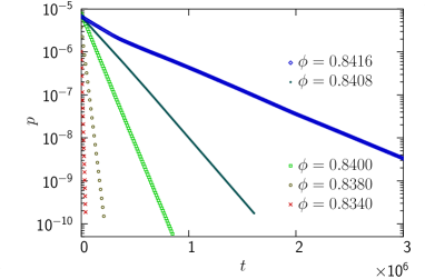
Figure 1: Examples of the pressure relaxation at different $\phi$. The figure shows the pressure relaxation after the shearing has been switched off. The preceeding shearings were performed at very low shear rates in order to stay close to the linear region; the densities and the initial shear rates were $(\phi,\dot{\gamma})=(0.8340,10^{-8})$, $(0.8380,10^{-8})$, $(0.8400,5\times 10^{-9})$, $(0.8408,2\times 10^{-9})$, $(0.8416,10^{-9})$. To determine the relaxation times, $\tau$, we fit pressure to an exponential decay, only using data with $p<10^{-7}$.

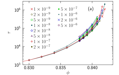
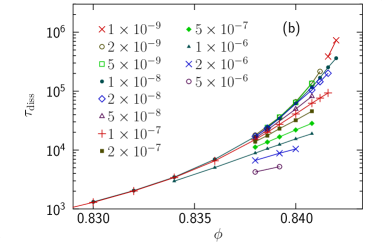
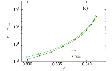
Figure 2: Relaxation time and dissipation time vs density. Panel (a) shows $\tau$ vs $\phi$ at several different shear rates. The data increases rapidly with increasing $\phi$ suggestive of a divergence at $\phi_{J}$. There is also a clear shear rate dependence, $\tau$ decreases when $\dot{\gamma}$ is decreased towards the hard disk limit, $\dot{\gamma}\to 0$. Panel (b) which shows $\tau_{\mathrm{diss}}$ vs $\phi$ also increases rapidly with $\phi_{J}$. The shear rate dependence is however the opposite; $\tau_{\mathrm{diss}}$ increases with decreasing $\dot{\gamma}$. Panel (c) shows a comparison of $\tau$ and $\tau_{\mathrm{diss}}$ which only includes the data with the lowest $\dot{\gamma}$ (i.e. closest to the hard disk limit). $\tau$ and $\tau_{\mathrm{diss}}$ behave essentially the same across this density interval, they are very close at the highest density close to $\phi_{J}$, but the (relative) difference increases with decreasing $\phi$.

III.1.2 Dissipation time

As a complement to the relaxation time, which is determined from the final decay of the pressure, we also introduce the “dissipation time” $\tau_{\mathrm{diss}}$, which is defined from the initial decay rate, just after the shearing has been turned off. For this quantity there is however no need to study the actual relaxations; at any moment the relaxation rate for the energy may be determined from the energy together with the dissipating power, giving $\tau^{\prime}=E/P_{\mathrm{diss}}$. In steady shear we may equate the dissipated power with the input power $P_{\mathrm{in}}=V\sigma\dot{\gamma}$, which gives $\tau^{\prime}=E/(\sigma\dot{\gamma})$ for the average dissipation time. As we want a quantity that may be directly compared to $\tau$—i.e. the decay time for pressure rather than the decay time for energy—we note that $p\sim\delta$ whereas $E\sim\delta^{2}$ which means that $p(t)\sim e^{-t/\tau}$ implies $E(t)\sim e^{-t/(\tau/2)}$, and that the two relaxation times differ by a factor of two. Our final expression for the dissipation time is therefore

$$\tau_{\mathrm{diss}}=2\frac{E}{\sigma\dot{\gamma}}.$$ (11)

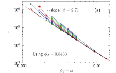
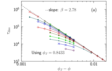
Figure 3: Divergence of $\tau$ and $\tau_{\mathrm{diss}}$. We here fix $\phi_{J}=0.8433$ and determine $\beta$ by fitting the few points of $\tau$ and $\tau_{\mathrm{diss}}$, respectively, with $\phi_{J}-\phi<0.006$ and sufficiently small $\dot{\gamma}$ to be close to the hard disk limit. (The points for $\phi=0.8420$ and $\dot{\gamma}=10^{-9}$ appear to be too far from the hard disk limit and are not included in the fits.)

Figure 2(b) shows $\tau_{\mathrm{diss}}$ against $\phi$ for several different shear rates. Just as for $\tau$ this quantity also appears to diverge as $\phi\to\phi_{J}$. The $\dot{\gamma}$-dependence is however different; $\tau_{\mathrm{diss}}$ decreases with increasing $\dot{\gamma}$, which means that the relative decrease of the energy is bigger in simulations at higher shear rates. The different behaviors of $\tau$ and $\tau_{\mathrm{diss}}$ is presumably because $\tau_{\mathrm{diss}}$ picks up contributions from all kinds of decay modes, and the faster modes are more excited when the system is driven with a higher shear rate. In contrast, $\tau$ only gets contributions from the slowest decay mode.

Figure 2(c) shows a comparison of $\tau$ and $\tau_{\mathrm{diss}}$. To eliminate effects due to the finite shear rate we only include the data at the smallest shear rate and exclude the data at $\phi=0.8420$, $\dot{\gamma}=10^{-9}$ which is clearly away from the $\dot{\gamma}\to 0$ limit.

III.1.3 Divergence

We are now ready to demonstrate one of the key results of the present paper, which is that both $\tau$ and $\tau_{\mathrm{diss}}$ diverge with the exponent $\beta$. From the definition of the dissipation time in Eq. (11) together with Eqs. (6) and (4), it follows directly that $\tau_{\mathrm{diss}}$ diverges with the exponent $\beta$:

$$\tau_{\mathrm{diss}}=\frac{E/\dot{\gamma}^{2}}{\sigma/\dot{\gamma}}\sim\frac{(\phi_{J}-\phi)^{-2\beta}}{(\phi_{J}-\phi)^{-\beta}}\sim(\phi_{J}-\phi)^{-\beta}.$$ (12)

That $\tau$ diverges in the same way follows from the very similar behaviors in Fig. 2(c) but in Sec. III.2.2 we will also argue for a direct connection between $\eta_{p}$ and $\tau$ by other means.

Figs. 3 show the determination of $\beta$ from $\tau$ and $\tau_{\mathrm{diss}}$. The determinations are based on the data points from in Fig. 2(c) very close to $\phi_{J}$, $\phi_{J}-\phi<0.006$. With only a few points with limited precision in a narrow interval of $\phi$, it is difficult to do a fit with both $\beta$ and $\phi_{J}$ as free parameters. We therefore instead determine $\beta$ after fixing the jamming density to $\phi_{J}=0.8433$Heussinger_Barrat:2009 ; Olsson_Teitel:gdot-scale ; Olsson_Teitel:jam-HB . The actual fits of $\tau$ and $\tau_{\mathrm{diss}}$ are shown in Figs. 3 and give similar values for the exponent: $\beta=2.71$ and $\beta=2.78$ in good agreement with earlier estimatesOlsson_Teitel:gdot-scale ; Olsson_Teitel:jam-HB ; DeGiuli:2014 .

III.2 Relations to hard disk simulations

In this Section we will relate the relaxation time $\tau$ to results from the study of the vibrational modes of sheared hard disksLerner-PNAS:2012 . Relations between these two approaches are expected since soft disk simulations at sufficiently low shear rates give vanishingly small overlaps and therefore should behave just as hard disks.

III.2.1 Relaxation time and the vibrational frequency

To motivate the relation between the relaxation time and the vibrational frequency we consider small displacements ${\bf u}_{i}$ from a zero-energy state. Written in terms of the vector ${\bf u}$, with $2N$ elements, and the stiffness matrix ${\cal M}$, such that the force (also a vector with $2N$ components) becomes $\epsilon{\cal M}{\bf u}$, the equation of motion for inertial dynamics may be written

$$m\frac{d^{2}{\bf u}}{dt^{2}}=\epsilon{\cal M}{\bf u}.$$ (13)

(We here consider a finite mass although our work is concerned with the overdamped limit of $m\to 0$, only to be able to relate to other approaches.) With eigenvalues $\lambda^{(k)}$ and eigenvectors ${\bf u}^{(k)}$, the force due to a general displacement field, ${\bf u}=\sum_{k}c_{k}{\bf u}^{(k)}$ becomes $\epsilon\sum_{k}\lambda^{(k)}c_{k}{\bf u}^{(k)}$ and the ansatz ${\bf u}(t)=\sum_{k}c_{k}{\bf u}^{(k)}\sin\omega_{k}t$ gives $\omega_{k}^{2}=-(\epsilon/m)\lambda^{(k)}$. However, below $\phi_{J}$ where the number of contacts is below the isostatic value there are modes with zero energy and $\omega_{k}=0$, which complicates the analysis. From the formalism for shearing of hard disks Lerner et al. Lerner-PNAS:2012 derived a matrix with the same eigenvalues as ${\cal M}$ except for these zero-energy modes. For that matrix the lowest frequency, $\omega_{\mathrm{min}}$, is always finite.

The relaxation may similarly be analyzed in terms of small displacements and for overdamped dynamics the equation of motion becomes

$$k_{d}\frac{d{\bf u}}{dt}=\epsilon{\cal M}{\bf u}.$$ (14)

The ansatz of an exponential decay, ${\bf u}(t)=\sum_{k}{\bf u}^{(k)}\exp(-t/\tau_{k})$ then gives $\tau_{k}^{-1}=-(\epsilon/k_{d})\lambda^{(k)}$. Taken together, Eqs. (13) and (14) give the desired relation between the relaxation time and the vibrational frequencies,

$$\tau_{k}=\frac{k_{d}}{m}\omega_{k}^{-2}.$$ (15)

Our largest $\tau_{k}$—the same as our relaxation time, $\tau$—then corresponds to the lowest frequency, $\omega_{\mathrm{min}}$.

$$\tau\sim\omega_{\mathrm{min}}^{-2}.$$ (16)

Our observation that there is only a single relaxation time that controls the decay corresponds well with the findingLerner-PNAS:2012 that the lowest frequency in the vibrational analysis is an isolated mode. If that were not the case, one would expect several decay modes with similar relaxation times and that would be seen through a curvature in the data in Fig. 1.

III.2.2 Relation to pressure

The formalism of LABEL:Lerner-PNAS:2012 gives the relation

$$\omega_{\mathrm{min}}^{-2}\sim\eta_{p},$$

to be valid in the hard disk limit. Together with Eq. (16) this leads us to expect that $\tau$ and $\eta_{p}$ should behave the same in the hard disk limit and Figs. 4 shows comparisons of $\tau$ and $\eta_{p}$ from our soft disk simulations with different shear rates. The data clearly approach one another as $\dot{\gamma}\to 0$.

Panel (a) shows $\tau$ together with $A_{p}\eta_{p}$ (where the constant is $A_{p}=36$) against $\phi$ for different $\dot{\gamma}$. Both quantities do indeed appear to approach the same curve in the $\dot{\gamma}\to 0$ limit, given by the dashed line, $f_{\tau}(\phi)\sim(\phi_{J}-\phi)^{-2.6}$. Panel (b) which shows the same data, but now relative to $f_{\tau}(\phi)$, serves as a strong confirmation of the expected equality and gives ample support for the expected direct proportionality between $\tau$ and $\eta_{p}$ in the hard disk limit. Recall that $\eta_{p}$ and $\tau$ are very different quantities as the first is determined at constant shearing whereas the second is from the relaxation rate of the pressure.

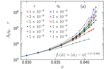
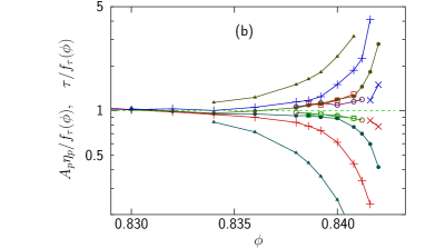
Figure 4: Comparison of $\tau$ and $\eta_{p}$ which, up to a constant prefactor, are expected to behave the same as $\dot{\gamma}\to 0$. Panel (a) shows the raw data, $\tau$, and $A_{p}\eta_{p}$, with the constant $A_{p}=36$. The data for large shear rates (solid triangles) are clearly different, but the respective points approach one another as $\dot{\gamma}\to 0$. The dashed line is $f_{\tau}(\phi)\sim(\phi_{J}-\phi)^{-\beta}$ with $\beta=2.60$. Panel (b) show the same data, but now divided by $f_{\tau}(\phi)$. The figure clearly suggests that the data should agree in the $\dot{\gamma}\to 0$ limit.

III.3 Contact number

III.3.1 Relaxation time and contact number

A key result from the study of static packings is that jamming in frictionless systems occurs when the coordination number is $z=z_{\mathrm{iso}}\equiv 2D$, which is the number needed for mechanical stability.Alexander:1998 This is however exact only in the absence of rattlers—particles that are not locked up at a fixed position as they have less than three contacts. To eliminate rattlers we follow LABEL:Lerner-PNAS:2012 and repeatedly remove all particles with less than three contacts. After removing the rattlers, $z_{1}$ is obtained as the average number of contacts of the remaining particles.

Following Lerner et al. Lerner-PNAS:2012 we show the individual determinations, $\tau_{1}$ against $\delta z_{1}\equiv z_{\mathrm{iso}}-z_{1}$ in Fig. 5(a). The figure gives strong evidence for an algebraic relation. For the vanishing of $\delta z_{1}$ we introduce $u_{z}$,

$$\delta z\sim(\phi_{J}-\phi)^{u_{z}}.$$ (17)

Together with $\tau\sim(\phi_{J}-\phi)^{-\beta}$ this gives a relation between the individual data points $\tau_{1}$ and $z_{1}$,

$$\tau_{1}\sim(\delta z_{1})^{-\beta/u_{z}},$$ (18)

and a fit of our data gives the exponent $\beta/u_{z}=2.69$. Since there is a curvature in the data that sets in around $\delta z_{1}=0.1$, only data with $\delta z_{1}<0.08$ were used in the fit. This result appears to be especially robust since it is obtained from a very simple fit of the raw data with no adjustable parameter. (Compare Fig. 3 where a determination of $\beta$ depends on the correct value of $\phi_{J}$.) Note also that there is no need to restrict the data to small shear rates of the initial simulation stage. As shown in Fig. 5(b) data for different $\dot{\gamma}$ do indeed fall on (or spread around) the same line. The explanation for this seems to be that both $\tau_{1}$ and $z_{1}$ are determined from configurations with almost vanishing overlaps, essentially in the hard disk limit, independent of the initial shear rate. Together with $\beta=2.70$Olsson_Teitel:gdot-scale this suggests $u_{z}=1$ whereas the somewhat smaller $\beta=2.58$ Olsson_Teitel:jam-HB which would imply $u_{z}\approx 0.96$, means that we cannot exclude the possibility that $u_{z}$ takes on a non-integral value.

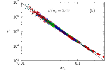
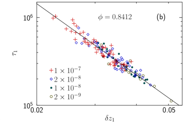
Figure 5: Corresponding values of $\tau_{1}$ and $\delta z_{1}$. Panel (a) shows 2719 corresponding values of $\tau_{1}$ and $\delta z_{1}$. Each point is from a relaxation that gives both a relaxation time $\tau_{1}$ and a final configuration from which the contact number $z_{1}$ is determined. The relaxation time clearly depends algebraically on $\delta z_{1}$—the distance to isostaticity. A fit of all data with $\delta z_{1}<0.08$ (1625 points) gives the exponent $\beta/u_{z}=2.69$. Panel (b) is a zoom-in with a more restricted set of data: $\phi=0.8412$ and four different shear rates. This shows that the points for different initial shear rates fall on a single curve.

Our result $\beta/u_{z}=2.69$ is in good agreement with LABEL:Lerner-PNAS:2012 who found $\beta/u_{z}=1/0.38=2.63$. A more recent paper by the same authorsDeGiuli:2014 , however, suggests $\beta/u_{z}=1/0.3\approx 3.3$ (their Fig. 5(c)). This new and lower exponent ($0.3<0.38$) is due to a curvature in their data, bending over from a larger slope for $\delta z>0.1$ to this lower slope for $\delta z<0.1$. This bending over at $\delta z_{1}\approx 0.1$ is similar to our Fig. 5(a), though the slopes are different. We cannot offer any explanation for this difference. (The effect in Fig. 8(a) below, which also leads to a larger value of $\beta/u_{z}$, doesn’t seem to be applicable in that case.)

As mentioned above the contact numbers were determined from the relaxed configurations with almost vanishing particle overlaps. To check if it would be possible to do a similar analysis of the configurations before the relaxations, we have also determined the corresponding starting values, $z_{1}^{\mathrm{start}}$, and to see how the relaxation process changes the contact number Fig. 6 shows the final contact number, $z_{1}$ against the corresponding starting values, $z_{1}^{\mathrm{start}}$. These data are obtained for $\phi=0.8412$, closely below $\phi_{J}$, and four different shear rates. From the figure we may draw a few different conclusions: (1) The contact number always decreases in the relaxation process. (2) This change is bigger for larger initial shear rates. (3) The final $z_{1}$ decreases slowly with decreasing initial shear rate. (4) The contact number of the starting configurations is sometimes above isostaticity, $z_{1}^{\mathrm{start}}>z_{\mathrm{iso}}$ whereas $z_{1}$ is always below. This last point makes clear that the analyses above, where the approach to jamming is seen by $z_{1}\to z_{\mathrm{iso}}$ can not be used with $z_{1}^{\mathrm{start}}$; it is only $z_{1}$ obtained from the relaxed configurations that approaches $z_{\mathrm{iso}}$ as jamming is approached.

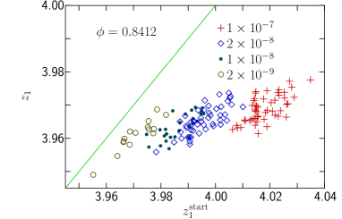
Figure 6: Change in contact number in the relaxation process. The figure shows contact numbers before and after the relaxation. The solid line is $z_{1}=z_{1}^{\mathrm{start}}$. The configurations are at density $\phi=0.8412$; the starting configurations are generated with four different initial shear rates. Both the initial $z_{1}^{\mathrm{start}}$ and $z_{1}$, obtained after the relaxation, are calculated after repeatedly removing all particles with less than three contacts.

III.3.2 Analysis of the CD₀ model

We have also applied the methods discussed above to the CD₀ model. These results are from a rather limited number of relaxations and no data very close to jamming, but they nevertheless give convincing results. Fig. 7 shows $\tau_{1}$ vs $\delta z_{1}$ just as in Fig. 5. The solid line, from fitting the data with $\delta z_{1}<0.08$, gives the exponent $\beta/u_{z}=2.63$. We note that this is very close to $\beta/u_{z}=2.69$ of the RD₀ model which gives support to the recent claimVagberg_OT:jam-cdrd that these two models have the same critical behavior. To facilitate a direct comparison, the fitting line in Fig. 5 is included as a dashed line in Fig. 7. The only difference appears to be that the the relaxation time for the CD₀ model is about a factor 1.5 larger than for the RD₀ model, for the same value of $\delta z_{1}$.

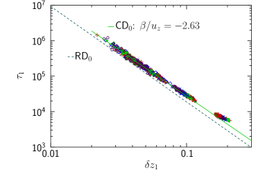
Figure 7: Determination of $\beta/u_{z}$ for the CD₀ model. By fitting data for $\delta z_{1}<0.08$ to Eq. (18) we determine $\beta/u_{z}=2.63$. We note that this is very close to $\beta/u_{z}=2.69$ of the RD₀ model.

III.3.3 Effect of large fluctuations

Figure 5 above displayed the individual data points $(\tau_{1},\delta z_{1})$, with different symbols for different simulation parameters $\phi$, $\dot{\gamma}$. An obvious way to show the same thing in a less crowded figure, would be to determine the arithmetic means of $\tau_{1}$ and $z_{1}$ for the different sets $(\phi,\dot{\gamma})$. We introduce the notation $\tau_{a}$ and $(\delta z)_{a}$ for these arithmetic means. ($\tau_{a}$ is thus just the ordinary average, $\tau$.) This kind of data is shown in Fig. 8(a), and it then turns out that the averaged data don’t behave quite the same as the individual points; the few points at the smallest $(\delta z)_{a}$ are now clearly off the solid line. The reason for this is that the $\tau_{1}$ for a certain combination of $\phi$, $\dot{\gamma}$ are spread over a finite range of $\delta z$ and since there is a power law relation between $\tau$ and $\delta z$, if one does the arithmetic average of this fixed phi data, one gets a point that does not lie on the same curve.

However, it turns out that things work differently—all the data fall on the line—when one instead plots the geometric means,

$$\tau_{g}(\phi,\dot{\gamma}) = \exp\left(\left<\ln\tau_{1}^{(\phi,\dot{\gamma})}\right>\right),$$ (19)

$$(\delta z)_{g}(\phi,\dot{\gamma}) = \exp\left(\left<\ln\delta z_{1}^{(\phi,\dot{\gamma})}\right>\right).$$ (20)

This data is shown in Fig. 8(b).

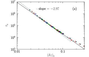
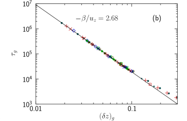
Figure 8: Mean values of $\tau_{1}$ and $\delta z_{1}$ determined in two different ways. Panel (a) shows the ordinary arithmetic mean values. For small $\delta z$ these points deviate clearly from the expected algebraic behavior. This phenomenon is due to the large spread of the data which appears close to jamming as is also described in conjuction with Figs. 9. Panel (b) which shows the geometric means, $\tau_{g}$, and $(\delta z)_{g}$ of the points $(\tau_{1},\delta z_{1})$ in Fig. 5(a) for the same $\phi$ and $\dot{\gamma}$. These points obey an algebraic behavior with the exponent $\beta/u_{z}=2.68$ in very good agreement with the analysis of the individual data points in Fig. 5(a).

To illustrate what happens when one averages data with a power law relation, Figs. 9 show the behavior of arithmetic and geometric means for some points on the line $y=x^{-3}$, on logarithmic and linear scales, respectively. The points labelled “arithmetic” and “geometric” are the respective averages of the open circles in the figures. In the left panel, which shows the data on logarithmic scales, the arithmetic average is again, just as in Fig. 8(a), clearly off the line. Though this could seem surprising, a plot with linear scales as in panel (b) directly shows that the arithmetic average cannot lie on that line.

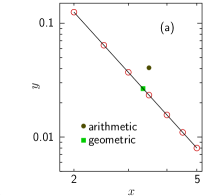
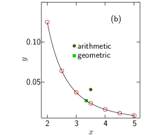
Figure 9: Illustration of the arithmetic mean and the geometric means for some points on the curve $y=x^{-3}$. From the figure with linear scale in panel (b) it is clear that one cannot expect the arithmetic mean to lie on top of the curve. As discussed in the text this effect only becomes important in cases where the relative variance is sizeable.

This effect is directly related to the big spread in the data around the average together with a power different from one. With points $y_{i}=y_{a}(1+\delta_{i})$ where $y_{a}$ is the arithmetic mean and $\delta_{i}$ the relative deviation from this mean, the variance is $\sigma_{y}^{2}=\left<y^{2}\right>-\left<y\right>^{2}=y_{a}^{2}\left<\delta_{i}^{2}\right>$. To second order in the deviations, the geometric mean becomes

$$y_{g} = \exp\left(\left<\ln[y_{a}(1+\delta_{i})]\right>\right)$$

$$\approx y_{a}\exp\left(\left<\delta_{i}-\delta_{i}^{2}/2\right>\right)\approx y_{a}(1-\left<\delta_{i}^{2}/2\right>),$$

and the ratio of the two different averages becomes

$$\frac{y_{g}}{y_{a}}=1-\frac{\sigma_{y}^{2}}{2y_{a}^{2}},$$ (21)

which means that the effects discussed here are important only when the fluctuations in the data are truly large.

III.3.4 Finite size dependence

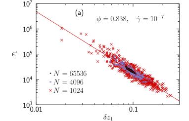
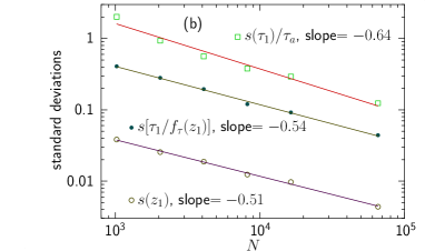
Figure 10: Finite size and the spread of the points $(\tau_{1},\delta z_{1})$ for $\phi=0.838$ and initial shear rate $\dot{\gamma}=10^{-7}$. Panel (a) which is $(\tau_{1},\delta z_{1})$ for three different system sizes shows that the points spread considerably more for smaller $N$. Panel (b) shows different quantitative measures of the spread of these data. The open circles are $s(z_{1})$—the standard deviation of $z_{1}$. Open squares are $s(\tau_{1})/\tau_{a}$. (The normalization by $\tau_{a}$ is to get quantities of the same order of magnitude). Solid dots are the standard deviation of $\tau_{1}/f_{\tau}(z_{1})$ which is the relative deviation of $\tau_{1}$ from the solid line in panel (a). Note that both the spread of $z_{1}$ and the spread around the solid line vanish as $1/\sqrt{N}$, as if the data were averages of $N$ independent samples.

We now examine the spread of $z_{1}$ and $\tau_{1}$, as in Fig. 5(b), around the solid line, with special focus on how this spread depends on the finite system size. For the finite size study we turn to a lower packing fraction, $\phi=0.838$. The reason for this is that, closer to $\phi_{J}$ (e.g. at $\phi=0.840$) some configurations for smaller sizes fail to reach zero energy in the relaxation step and get jammed with $z>z_{\mathrm{iso}}$, and such events badly complicate the analysis.

Fig. 10 which is $\tau_{1}$ vs $z_{1}$ for $\phi=0.838$, the initial shear rate $\dot{\gamma}=10^{-7}$, and the three sizes, $N=1024$, $N=4096$, and 65536, clearly shows that these data spread more for smaller $N$. Note that the data in Fig. 10 for all different sizes have a common behavior, $\tau_{1}\approx f_{\tau}(z_{1})\equiv A_{\tau}(\delta z_{1})^{-b}$. The exponent $b=2.40$ is an effective exponent which differs from $\beta/u_{z}=2.69$ (obtained in Fig. 5) since we here make use of data with larger $\delta z_{1}$.

We introduce three different measures to characterize the spread of this data. Two straightforward measures are $s(z_{1})$ and $s(\tau_{1})$ which are the standard deviations of the data. Another measure is the spread of $\tau_{1}$ away from the line, i.e. the value predicted from the known $z_{1}$, $s[\tau_{1}/f_{\tau}(z_{1})]$. These three quantities are shown in Fig. 10(b) for number of particles ranging from $N=1024$ through 65536. To interpret this data we first recall that the standard deviation of averages of $N$ independent samples is $\sim N^{-1/2}$. We find that both $s(z_{1})$ and $s(\tau_{1})/\tau_{a}$ vanish with the exponents $-0.54$ and $-0.51$ in excellent agreement with this expectation. For $s[\tau_{1}/f_{\tau}(z_{1})]$ we find a somewhat more complicated behaviour with a larger exponent, $-0.64$, and a questionable fit to the data. Taken together our data suggest an interpretation where both the spread of $z_{1}$ and the spread of $\tau_{1}$ around $f_{\tau}(z_{1})$ are controlled by independent simple stochastic processes.

IV Discussion

The relaxation dynamics around the jamming transition has been studied before, but with a rather different approach Hatano:2009 : the configurations were first generated randomly, then relaxed to a zero-energy state with the conjugate gradient method, and after that perturbed by a pure affine shear deformation. The relaxation time was then determined from the relaxation of such initial states by fitting the shear stress to $\sigma(\phi,t)\sim t^{-\alpha}e^{-t/\tau}$ with $\alpha=0.55(5)$, and the relaxation time was found to diverge as $\tau\sim(\phi_{J}-\phi)^{-\zeta}$ with $\zeta=3.3(1)$. This exponent is clearly bigger than our $\beta\approx 2.7$. One possible explanation for this difference is that we in the present study get data in the limit of vanishing shear rate in the preparation step (i.e. $\dot{\gamma}\to 0$ in the steady state shearing), whereas they in their work apply the pure shear deformation suddenly, which is more like a rapid shearing. Indeed, as shown in Fig. 3(a) any given fixed shear rate would give too large values for $\tau$ as one gets close to $\phi_{J}$, and from analyses of such data one would expect to get too high values of the exponent for the divergence.

We finally want to stress two consequences of the presented results: We first stress that the above results taken together suggest that $\tau$ is a fundamental quantity that controls the overlap $\delta/\dot{\gamma}$ and thereby is behind the divergence of other quantites like $\eta_{p}$ and $\eta$. For a detailed argument we consider the $\dot{\gamma}\to 0$ limit where $\tau_{\mathrm{diss}}\approx\tau$ and the $N\to\infty$ limit where the spread of $z_{1}$ and $\tau_{1}$ vanish. A given $\phi$ then leads to a well-defined $\delta z$ which in turn implies a well-defined $\tau$ and $\tau_{\mathrm{diss}}\approx\tau$. With the additional assumption of a given value for the dimensionless friction, $\mu\equiv\sigma/p$, power balance between the input power $P_{\mathrm{in}}=\sigma\dot{\gamma}\sim\mu\delta\dot{\gamma}$ and the dissipated power $P_{\mathrm{diss}}=E/\tau_{\mathrm{diss}}\sim\delta^{2}/\tau_{\mathrm{diss}}$ gives $\delta/\dot{\gamma}\sim\tau_{\mathrm{diss}}\mu$. This therefore provides a very direct link between the relaxation times and $\eta_{p}\sim\delta/\dot{\gamma}$.

Seconly, we note that the relaxation time $\tau$ we have defined here has a different scaling exponent than does the time scale associated with rescaling the shear strain rate $\dot{\gamma}$. From Eq. (5) for the $\dot{\gamma}\to 0$ limit and dimensional arguments one would expect the deviations due to a finite $\dot{\gamma}$ to scale as

$$\eta_{p}(\phi,\dot{\gamma})/|\delta\phi|^{-\beta}\sim g(\dot{\gamma}\tau)\sim g(\dot{\gamma}/|\delta\phi|^{\beta}),\quad\mbox{(naive)},$$ (22)

where the scaling function $\lim_{x\to 0}g(x)=$ const (for the hard disk limit) and the deviations being controlled by $\dot{\gamma}\tau$. This is however not the case. As shown in Eq. (9) the data scale with $g(\dot{\gamma}/|\delta\phi|^{z\nu})$ where $z\nu=\beta+y$, $y\approx 1.1$, which thus is clearly different from the behavior expected from dimensional analysis. We hope to be able to return to this question elsewhere.

V Summary

To summarize, we have done extensive two-step simulations, first shearing the system at different constant shear rates and then stopping the shearing and letting the system relax. At late times of this relaxation, both energy and pressure decay exponentially, and we define the relaxation time, $\tau$, to be the time constant of the exponential decay of the pressure. We similarly define the “dissipation time” from the initial decay immediately after the shearing is turned off.

We then show that these two times behave very similarly when considering the limit of low shear rates, but also that their respective shear rate dependencies are opposite. From the expression for $\tau_{\mathrm{diss}}$, Eq. (11), it follows immediately that $\tau_{\mathrm{diss}}$ diverges with the exponent $\beta$—the same divergence as for $\eta_{p}=p/\dot{\gamma}$—and this is also corroborated by the $\phi$-dependence of $\tau$ and $\tau_{\mathrm{diss}}$ in the small-$\dot{\gamma}$ limit.

We also show that the relaxation time is directly related to the lowest vibrational frequency of hard disk systemsLerner-PNAS:2012 , and, furthermore, that this suggests a relation between $\tau$ and $\eta_{p}$, which should be valid in the small $\dot{\gamma}$ limit. Fig. 4, provide ample evidence that this actually is the case.

We then turn to a thorough study of the relation between the contact number and the relaxation time. The contact number is a key quantity in the field of jamming and we follow LABEL:Lerner-PNAS:2012 and determine the contact number after removing rattlers. With $\tau_{1}$ and $z_{1}$ from individual measurements, $\tau_{1}$ depends algebraically on the distance from isostaticity $\delta z_{1}=z_{\mathrm{iso}}-z_{1}$, $\tau_{1}\sim(\delta z_{1})^{\beta/u_{z}}$, with $\beta/u_{z}\approx 2.69$.

The same analysis applied to the CD₀ model gives essentially the same exponent, $\beta/u_{z}\approx 2.63$, which provides additional evidenceVagberg_OT:jam-cdrd that the CD₀ and the RD₀ models are in the same universality class. We consider these analysis to be especially robust as they are entirely straightforward and do not require data obtained at very low shear rates.

We then turn to effects of the spread of the individual $\tau_{1}$ for a fixed set of parameters $\phi$, $\dot{\gamma}$, around its average. We first point out that the ordinary arithmetic mean may be problematic and that a geometric mean actually in some respects works better. We then consider the finite size effect where we find that the spread of both the relaxation time and the coordination number go as $1/\sqrt{N}$, just as expected for the statistics of $N$ independent variables.

I thank S. Teitel for many discussions and a critical reading of the manuscript. This work was supported by the Swedish Research Council Grant No. 2010-3725. Simulations were performed on resources provided by the Swedish National Infrastructure for Computing (SNIC) at PDC and HPC2N.

References

- (1) A. J. Liu and S. R. Nagel, Nature (London) 396, 21 (1998)
- (2) C. S. O’Hern, L. E. Silbert, A. J. Liu, and S. R. Nagel, Phys. Rev. E 68, 011306 (2003)
- (3) P. Chaudhuri, L. Berthier, and S. Sastry, Phys. Rev. Lett. 104, 165701 (Apr 2010)
- (4) D. Vågberg, D. Valdez-Balderas, M. Moore, P. Olsson, and S. Teitel, Phys. Rev. E 83, 030303(R) (2011)
- (5) P. Olsson and S. Teitel, Phys. Rev. Lett. 99, 178001 (2007)
- (6) T. Hatano, J. Phys. Soc. Jpn. 77, 123002 (2008)
- (7) T. Hatano(2008), arXiv:0804.0477
- (8) M. Otsuki and H. Hayakawa, Phys. Rev. E 80, 011308 (2009)
- (9) T. Hatano, Phys. Rev. E 79, 050301 (2009)
- (10) T. Hatano, Prog. Theor. Phys. Suppl. 184, 143 (2010)
- (11) B. P. Tighe, E. Woldhuis, J. J. C. Remmers, W. van Saarloos, and M. van Hecke, Phys. Rev. Lett. 105, 088303 (2010)
- (12) C. Heussinger and J.-L. Barrat, Phys. Rev. Lett. 102, 218303 (2009)
- (13) C. Heussinger, P. Chaudhuri, and J.-L. Barrat, Soft Matter 6, 3050 (2010)
- (14) E. Lerner, G. Düring, and M. Wyart, PNAS 109, 4798 (2012)
- (15) G. Düring, E. Lerner, and M. Wyart, Phys. Rev. E 89, 022305 (2014)
- (16) E. DeGiuli, G. Düring, E. Lerner, and M. Wyart, arXiv:1410.3535
- (17) D. Vågberg, P. Olsson, and S. Teitel, Phys. Rev. Lett. 113, 148002 (2014)
- (18) D. J. Evans and G. P. Morriss, Statistical Mechanics of Nonequilibrium Liquids (Academic Press, London, 1990)
- (19) D. J. Durian, Phys. Rev. Lett. 75, 4780 (Dec 1995)
- (20) S. Tewari, D. Schiemann, D. J. Durian, C. M. Knobler, S. A. Langer, and A. J. Liu, Phys. Rev. E 60, 4385 (1999)
- (21) B. Andreotti, J.-L. Barrat, and C. Heussinger, Phys. Rev. Lett. 109, 105901 (2012)
- (22) P. Olsson and S. Teitel, Phys. Rev. E 83, 030302(R) (2011)
- (23) T. Kawasaki, D. Coslovich, A. Ikeda, and L. Berthier, Phys. Rev. E 91, 012203 (2015)
- (24) P. Olsson and S. Teitel, Phys. Rev. Lett. 109, 108001 (2012)
- (25) S. Alexander, Physics Reports 296, 65 (1998)