Cross-validation of matching correlation analysis by resampling matching weights

Abstract

The strength of association between a pair of data vectors is represented by a nonnegative real number, called matching weight. For dimensionality reduction, we consider a linear transformation of data vectors, and define a matching error as the weighted sum of squared distances between transformed vectors with respect to the matching weights. Given data vectors and matching weights, the optimal linear transformation minimizing the matching error is solved by the spectral graph embedding of Yan et al. (2007). This method is a generalization of the canonical correlation analysis, and will be called as matching correlation analysis (MCA). In this paper, we consider a novel sampling scheme where the observed matching weights are randomly sampled from underlying true matching weights with small probability, whereas the data vectors are treated as constants. We then investigate a cross-validation by resampling the matching weights. Our asymptotic theory shows that the cross-validation, if rescaled properly, computes an unbiased estimate of the matching error with respect to the true matching weights. Existing ideas of cross-validation for resampling data vectors, instead of resampling matching weights, are not applicable here. MCA can be used for data vectors from multiple domains with different dimensions via an embarrassingly simple idea of coding the data vectors. This method will be called as cross-domain matching correlation analysis (CDMCA), and an interesting connection to the classical associative memory model of neural networks is also discussed.

t1 Supported in part by JSPS KAKENHI Grant (24300106, 26120523).

1 Introduction

We have $N$ data vectors of $P$ dimensions. Let $\bm{x}_{1},\ldots,\bm{x}_{N}\in\mathbb{R}^{P}$ be the data vectors, and $\bm{X}=(\bm{x}_{1},\ldots,\bm{x}_{N})^{T}\in\mathbb{R}^{N\times P}$ be the data matrix. We also have matching weights between the data vectors. Let $w_{ij}=w_{ji}\geq 0$, $i,j=1,\ldots,N$, be the matching weights, and $\bm{W}=(w_{ij})\in\mathbb{R}^{N\times N}$ be the matching weight matrix. The matching weight $w_{ij}$ represents the strength of association between $\bm{x}_{i}$ and $\bm{x}_{j}$. For dimensionality reduction, we will consider a linear transformation from $\mathbb{R}^{P}$ to $\mathbb{R}^{K}$ for some $K\leq P$ as

$$\bm{y}_{i}=\bm{A}^{T}\bm{x}_{i},\quad i=1,\ldots,N,$$

or $\bm{Y}=\bm{X}\bm{A}$, where $\bm{A}\in\mathbb{R}^{P\times K}$ is the linear transformation matrix, $\bm{y}_{1},\ldots,\bm{y}_{N}\in\mathbb{R}^{K}$ are the transformed vectors, and $\bm{Y}=(\bm{y}_{1},\ldots,\bm{y}_{N})^{T}\in\mathbb{R}^{N\times K}$ is the transformed matrix. Observing $\bm{X}$ and $\bm{W}$, we would like to find $\bm{A}$ that minimizes the matching error

$$\phi=\frac{1}{2}\sum_{i=1}^{N}\sum_{j=1}^{N}w_{ij}\|\bm{y}_{i}-\bm{y}_{j}\|^{2}$$

under some constraints. We expect that the distance between $\bm{y}_{i}$ and $\bm{y}_{j}$ will be small when $w_{ij}$ is large, so that the locations of transformed vectors represent both the locations of the data vectors and the associations between data vectors. The optimization problem for finding $\bm{A}$ is solved by the spectral graph embedding for dimensionality reduction of Yan et al. (2007). Similarly to principal component analysis (PCA), the optimal solution is obtained as the eigenvectors of the largest $K$ eigenvalues of some matrix computed from $\bm{X}$ and $\bm{W}$. In Section 3, this method will be formulated by specifying the constraints on the transformed vectors and also regularization terms for numerical stability. We will call the method as matching correlation analysis (MCA), since it is a generalization of the classical canonical correlation analysis (CCA) of Hotelling (1936). The matching error will be represented by matching correlations of transformed vectors, which correspond to the canonical correlations of CCA.

MCA will be called as cross-domain matching correlation analysis (CDMCA) when we have data vectors from multiple domains with different sample sizes and different dimensions. Let $D$ be the number of domains, and $d=1,\ldots,D$ denote each domain. For example, domain $d=1$ may be for image feature vectors, and domain $d=2$ may be for word vectors computed by word2vec (Mikolov et al., 2013) from texts, where the matching weights between the two domains may represent tags of images in a large dataset, such as Flickr. From domain $d$, we get data vectors $\bm{x}^{(d)}_{i}\in\mathbb{R}^{p_{d}}$, $i=1,\ldots,n_{d}$, where $n_{d}$ is the number of data vectors, and $p_{d}$ is the dimension of the data vector. Typically, $p_{d}$ is hundreds, and $n_{d}$ is thousands to millions. We would like to retrieve relevant words from an image query, and alternatively retrieve images from a word query. Given matching weights across/within domains, we attempt to find linear transformations of data vectors from multiple domains to a “common space” of lower dimensionality so that the distances between transformed vectors well represent the matching weights. This problem is solved by an embarrassingly simple idea of coding the data vectors, which is similar to that of Daumé III (2009). Each data vector from domain $d$ is represented by an augmented data vector $\bm{x}_{i}$ of dimension $P=\sum_{d=1}^{D}p_{d}$, where only $p_{d}$ dimensions are for the original data vector and the rest of $P-p_{d}$ dimensions are padded by zeros. In the case of $D=2$ with $p_{1}=2$, $p_{2}=3$, say, a data vector $(1,2)^{T}$ of domain 1 is represented by $(1,2,0,0,0)^{T}$, and $(3,4,5)^{T}$ of domain 2 is represented by $(0,0,3,4,5)^{T}$. The number of total augmented data vectors is $N=\sum_{d=1}^{D}n_{d}$. Note that the above mentioned “embarrassingly simple coding” is not actually implemented by padding zeros in computer software; only the nonzero elements are stored in memory, and CDMCA is in fact implemented very efficiently for sparse $\bm{W}$. CDMCA is illustrated in a numerical example of Section 2. CDMCA is further explained in Appendix A.1, and an interesting connection to the classical associative memory model of neural networks (Kohonen, 1972; Nakano, 1972) is also discussed in Appendix A.2.

CDMCA is solved by applying the single-domain version of MCA described in Section 3 to the augmented data vectors, and thus we only discuss the single-domain version in this paper. This formulation of CDMCA includes a wide class of problems of multivariate analysis, and similar approaches are very popular recently in pattern recognition and vision (Correa et al., 2010; Yuan et al., 2011; Kan et al., 2012; Shi et al., 2013; Wang et al., 2013; Gong et al., 2014; Yuan and Sun, 2014). CDMCA is equivalent to the method of Nori, Bollegala and Kashima (2012) for multinomial relation prediction if the matching weights are defined by cross-products of the binary matrices representing relations between objects and instances. CDMCA is also found in Huang et al. (2013) for the case of $D=2$. CDMCA reduces to the multi-set canonical correlation analysis (MCCA) (Kettenring, 1971; Takane, Hwang and Abdi, 2008; Tenenhaus and Tenenhaus, 2011) when $n_{1}=\cdots=n_{D}$ with cross-domain matching weight matrices being proportional to the identity matrix. It becomes the classical CCA by further letting $D=2$, or it becomes PCA by letting $p_{1}=p_{2}=\cdots=p_{D}=1$.

In this paper, we discuss a cross-validation method for computing the matching error of MCA. In Section 4, we will define two types of matching errors, i.e., fitting error and true error, and introduce cross-validation (cv) error for estimating the true error. In order to argue distributional properties of MCA, we consider the following sampling scheme. First, the data vectors are treated as constants. Similarly to the explanatory variables in regression analysis, we perform conditional inference given data matrix $\bm{X}$, although we do not avoid assuming that $\bm{x}_{i}$’s are sampled from some probability distribution. Second, the matching weights $w_{ij}$ are randomly sampled from underlying true matching weights $\bar{w}_{ij}$ with small probability $\epsilon>0$. The value of $\epsilon$ is unknown and it should not be used in our inference. Let $z_{ij}=z_{ji}\in\{0,1\}$, $i,j=1,\ldots,N$, be samples from Bernoulli trial with success probability $\epsilon$, where the number of independent elements is $N(N+1)/2$ due to the symmetry. Then the observed matching weights are defined as

$$w_{ij}=z_{ij}\bar{w}_{ij},\quad P(z_{ij}=1)=\epsilon.$$ (1)

The true matching weight matrix $\bm{\bar{W}}=(\bar{w}_{ij})\in\mathbb{R}^{N\times N}$ is treated as an unknown constant matrix with elements $\bar{w}_{ij}=\bar{w}_{ji}\geq 0$. This setting will be appropriate for a large-scale data, such as those obtained automatically from the web, where only a small portion $\bm{W}$ of the true association $\bm{\bar{W}}$ may be obtained as our knowledge.

In Section 4.2, we will consider a resampling scheme corresponding to (1). For the cross-validation, we resample $\bm{W}^{*}$ from $\bm{W}$ with small probability $\kappa>0$, whereas $\bm{X}$ is left untouched. Our sampling/resampling scheme is very unique in the sense that the source of randomness is $\bm{W}$ instead of $\bm{X}$, and existing results of cross-validation for resampling from $\bm{X}$ such as Stone (1977) and Golub, Heath and Wahba (1979) are not applicable here. The traditional method of resampling data vectors is discussed in Section 4.3.

The true error is defined with respect to the unknown $\bm{\bar{W}}$, and the fitting error is defined with respect to the observed $\bm{W}$. We would like to look at the true error for finding appropriate values of the regularization terms (regularization parameters are generally denoted as $\gamma$ throughout) and the dimension $K$ of the transformed vectors. However, the true error is unavailable, and the fitting error is biased for estimating the true error. The main thrust of this paper is to show asymptotically that the cv error, if rescaled properly, is an unbiased estimator of the true error. The value of $\epsilon$ is unnecessary for computing the cv error, but $\bm{W}$ should be a sparse matrix. The unbiasedness of the cv error is illustrated by a simulation study in Section 5, and it is shown theoretically by the asymptotic theory of $N\to\infty$ in Section 6.

2 Illustrative example

Let us see an example of CDMCA applied to the MNIST database of handwritten digits (see Appendix B.1 for the experimental details). The number of domains is $D=3$ with the number of vectors $n_{1}=60,000$, $n_{2}=10$, $n_{3}=3$, and dimensions $p_{1}=2784$, $p_{2}=100$, $p_{3}=50$. The handwritten digit images are stored in domain $d=1$, while domain $d=2$ is for the digit labels “zero”, “one”, … , “nine”, and domain $d=3$ is for attribute labels “even”, “odd”, “prime”. This CDMCA is also interpreted as MCA with $N=60,013$ and $P=2934$.

The elements of $\bm{\bar{W}}$ are simply the indicator variables (called dummy variables in statistics) of image labels. Instead of working on $\bm{\bar{W}}$, here we made $\bm{W}$ by sampling 20% of the elements from $\bm{\bar{W}}$ for illustrating how CDMCA works. The optimal $\bm{A}$ is computed from $\bm{W}$ using the method described in Section 3.3 with regularization parameter $\gamma_{M}=0.1$. The data matrix $\bm{X}$ is centered, and the transformed matrix $\bm{Y}$ is rescaled. The first and second elements of $\bm{y}_{i}$, namely, $(y_{i1},y_{i2})$, $i=1,\ldots,N$, are shown in Fig. 1. For the computation of $\bm{A}$, we do not have to specify the value of $K$ in advance. Similar to PCA, we first solve the optimal $\bm{A}=(\bm{a}^{1},\ldots,\bm{a}^{P})\in\mathbb{R}^{P\times P}$ for the case of $K=P$, then take the first $K$ columns to get the optimal $\bm{A}=(\bm{a}^{1},\ldots,\bm{a}^{K})\in\mathbb{R}^{P\times K}$ for any $K\leq P$. We observe that images and labels are placed in the common space so that they represent both $\bm{X}$ and $\bm{W}$. Given a digit image, we may find the nearest digit label or attribute label to tell what the image represents.

The optimal $\bm{A}$ of $K=9$ is then computed for several $\gamma_{M}$ values. For each $\bm{A}$, the 10000 images of test dataset are projected to the common space and the digit labels and attribute labels are predicted. We observe in Fig. 2(a) that the classification errors become small when the regularization parameter is around $\gamma_{M}=0.1$. Since $\bm{x}_{i}$ does not contribute to $\bm{A}$ if $\sum_{j=1}^{N}w_{ij}=0$, these error rates are computed using only 20% of $\bm{X}$; they improve to 0.0359 ($d=2$) and 0.0218 ($d=3$) if $\bm{\bar{W}}$ is used for the computation of $\bm{A}$ with $K=11$ and $\gamma_{M}=0$.

It is important to choose an appropriate value of $\gamma_{M}$ for minimizing the classification error. We observe in Fig. 2(b) that the curve of the true matching error of the test dataset is similar to the curves of the classification errors. However, the fitting error wrongly suggests that a smaller $\gamma_{M}$ value would be better. Here, the fitting error is the matching error computed from the training dataset, and it underestimates the true matching error. On the other hand, the matching error computed by the cross-validation method of Section 4.2 correctly suggests that $\gamma_{M}=0.1$ is a good choice.

3 Matching correlation analysis

3.1 Matching error and matching correlation

Let $\bm{M}\in\mathbb{R}^{N\times N}$ be the diagonal matrix of row (column) sums of $\bm{W}$.

$$\bm{M}=\mathop{\rm diag}\nolimits(m_{1},\ldots,m_{N}),\quad m_{i}=\sum_{j=1}^{N}w_{ij}.$$

This is also expressed as $\bm{M}=\mathop{\rm diag}\nolimits(\bm{W}\bm{1}_{N})\in\mathbb{R}^{N\times N}$ using $\bm{1}_{N}\in\mathbb{R}^{N}$, the vector with all elements one. $\bm{M}-\bm{W}$ is sometimes called as the graph Laplacian. This notation will be applied to other weight matrices, say, $\bm{\bar{M}}$ for $\bm{\bar{W}}$. Key notations are shown in Table 1.

Column vectors of matrices will be denoted by superscripts. For example, the $k$-th component of $\bm{Y}=(y_{ik};\,i=1,\ldots,N,\,k=1,\ldots,K)$ is $\bm{y}^{k}=(y_{1k},\ldots,y_{Nk})^{T}\in\mathbb{R}^{N}$ for $k=1,\ldots,K$, and we write $\bm{Y}=(\bm{y}^{1},\ldots,\bm{y}^{K})$. Similarly, $\bm{X}=(\bm{x}^{1},\ldots,\bm{x}^{P})$ with $\bm{x}^{k}\in\mathbb{R}^{N}$, and $\bm{A}=(\bm{a}^{1},\ldots,\bm{a}^{K})$ with $\bm{a}^{k}\in\mathbb{R}^{P}$. The linear transformation is now written as $\bm{y}^{k}=\bm{X}\bm{a}^{k}$, $k=1,\ldots,K$.

The matching error of the $k$-th component $\bm{y}^{k}$ is defined by

$$\phi_{k}=\frac{1}{2}\sum_{i=1}^{N}\sum_{j=1}^{N}w_{ij}(y_{ik}-y_{jk})^{2},$$

and the matching error of all the components is $\phi=\sum_{k=1}^{K}\phi_{k}$. By noticing $\bm{W}=\bm{W}^{T}$, the matching error is rewritten as

$$\begin{split}\phi_{k}&=\frac{1}{2}\sum_{i=1}^{N}m_{i}y_{ik}^{2}+\frac{1}{2}\sum_{j=1}^{N}m_{j}y_{jk}^{2}-\sum_{i=1}^{N}\sum_{j=1}^{N}w_{ij}y_{ik}y_{jk}\\ &=\bm{y}^{k\,T}(\bm{M}-\bm{W})\bm{y}^{k}.\end{split}$$

Let us specify constraints on $\bm{Y}$ as

$$\bm{y}^{k\,T}\bm{M}\bm{y}^{k}=\sum_{i=1}^{N}m_{i}y_{ik}^{2}=1,\quad k=1,\ldots,K.$$ (2)

In other words, the weighted variance of $y_{1k},\ldots,y_{Nk}$ with respect to the weights $m_{1},\ldots,m_{N}$ is fixed as a constant. Note that we say “variance” or “correlation” although variables are not centered explicitly throughout. The matching error is now written as

$$\phi_{k}=1-\bm{y}^{k\,T}\bm{W}\bm{y}^{k}.$$

We call $\bm{y}^{k\,T}\bm{W}\bm{y}^{k}$ as the matching (auto) correlation of $\bm{y}^{k}$.

More generally, the matching error between the $k$-th component $\bm{y}^{k}$ and $l$-th component $\bm{y}^{l}$ for $k,l=1,\ldots,K$, is defined by

$$\frac{1}{2}\sum_{i=1}^{N}\sum_{j=1}^{N}w_{ij}(y_{ik}-y_{jl})^{2}=1-\bm{y}^{k\,T}\bm{W}\bm{y}^{l},$$

and the matching (cross) correlation between $\bm{y}^{k}$ and $\bm{y}^{l}$ is defined by $\bm{y}^{k\,T}\bm{W}\bm{y}^{l}$. This is analogous to the weighted correlation $\bm{y}^{k\,T}\bm{M}\bm{y}^{l}$ with respect to the weights $m_{1},\ldots,m_{N}$, but a different measure of association between $\bm{y}^{k}$ and $\bm{y}^{l}$. It is easily verified that $|\bm{y}^{k\,T}\bm{W}\bm{y}^{l}|\leq 1$ as well as $|\bm{y}^{k\,T}\bm{M}\bm{y}^{l}|\leq 1$. The matching errors reduce to zero when the corresponding matching correlations approach 1.

A matching error not smaller than one, i.e., $\phi_{k}\geq 1$, may indicate the component $\bm{y}^{k}$ is not appropriate for representing $\bm{W}$. In other words, the matching correlation should be positive: $\bm{y}^{k\,T}\bm{W}\bm{y}^{k}>0$. For justifying the argument, let us consider the elements $y_{ik}$, $i=1,\ldots,N$, are independent random variables with mean zero. Then $E(\bm{y}^{k\,T}\bm{W}\bm{y}^{k})=\sum_{i=1}^{N}w_{ii}V(y_{ik})=0$ if $w_{ii}=0$. Therefore random components, if centered properly, give the matching error $\phi_{k}\approx 1$.

3.2 The spectral graph embedding for dimensionality reduction

We would like to find the linear transformation matrix $\bm{\hat{A}}$ that minimizes $\phi=\sum_{k=1}^{K}\phi_{k}$. Here symbols are denoted with hat like $\bm{\hat{Y}}=\bm{X}\bm{\hat{A}}$ to make a distinction from those defined in Section 3.3. Define $P\times P$ symmetric matrices

$$\bm{\hat{G}}=\bm{X}^{T}\bm{M}\bm{X},\quad\bm{\hat{H}}=\bm{X}^{T}\bm{W}\bm{X}.$$

Then, we consider the optimization problem:

$$\mbox{Maximize}\quad\mathop{\rm tr}\nolimits(\bm{\hat{A}}^{T}\bm{\hat{H}}\bm{\hat{A}})\quad\mbox{with respect to}\quad\bm{\hat{A}}\in\mathbb{R}^{P\times K}$$ (3)

$$\mbox{subject to}\quad\bm{\hat{A}}^{T}\bm{\hat{G}}\bm{\hat{A}}=\bm{I}_{K}.$$ (4)

The objective function $\mathop{\rm tr}\nolimits(\bm{\hat{A}}^{T}\bm{\hat{H}}\bm{\hat{A}})=\sum_{k=1}^{K}\bm{\hat{y}}^{k\,T}\bm{W}\bm{\hat{y}}^{k}$ is the sum of matching correlations of $\bm{\hat{y}}^{k}$, $k=1,\ldots,K$, and thus (3) is equivalent to the minimization of $\phi$ as we wished. The constraints in (4) are $\bm{\hat{y}}^{k\,T}\bm{M}\bm{\hat{y}}^{l}=\delta_{kl}$, $k,l=1,\ldots,K$. In addition to (2), we assumed that $\bm{\hat{y}}^{k}$, $k=1,\ldots,K$, are uncorrelated each other to prevent $\bm{\hat{a}}^{1},\ldots,\bm{\hat{a}}^{K}$ degenerating to the same vector.

The optimization problem mentioned above is the same formulation as the spectral graph embedding for dimensionality reduction of Yan et al. (2007). A difference is that $\bm{W}$ is specified by external knowledge in our setting, while $\bm{W}$ is often specified from $\bm{X}$ in the graph embedding literature. Similar optimization problems are found in the spectral graph theory (Chung, 1997), the normalized graph Laplacian (Von Luxburg, 2007), or the spectral embedding (Belkin and Niyogi, 2003) for the case of $\bm{X}=\bm{I}_{N}$.

3.3 Regularization and rescaling

We introduce regularization terms $\Delta\bm{G}$ and $\Delta\bm{H}$ for numerical stability. They are $P\times P$ symmetric matrices, and added to $\bm{\hat{G}}$ and $\bm{\hat{H}}$. We will replace $\bm{\hat{G}}$ and $\bm{\hat{H}}$ in the optimization problem with

$$\bm{G}=\bm{\hat{G}}+\Delta\bm{G},\quad\bm{H}=\bm{\hat{H}}+\Delta\bm{H}.$$

The same regularization terms are considered in Takane, Hwang and Abdi (2008) for MCCA. We may write $\Delta\bm{G}=\gamma_{M}\bm{L}_{M}$ and $\Delta\bm{H}=\gamma_{W}\bm{L}_{W}$ with prespecified matrices, say, $\bm{L}_{M}=\bm{L}_{W}=\bm{I}_{P}$, and attempt to choose appropriate values of the regularization parameters $\gamma_{M},\gamma_{W}\in\mathbb{R}$.

We then work on the optimization problem:

$$\mbox{Maximize}\quad\mathop{\rm tr}\nolimits(\bm{A}^{T}\bm{H}\bm{A})\quad\mbox{with respect to}\quad\bm{A}\in\mathbb{R}^{P\times K}$$ (5)

$$\mbox{subject to}\quad\bm{A}^{T}\bm{G}\bm{A}=\bm{I}_{K}.$$ (6)

For the solution of the optimization problem, we denote $\bm{G}^{1/2}\in\mathbb{R}^{P\times P}$ be one of the matrices satisfying $(\bm{G}^{1/2})^{T}\bm{G}^{1/2}=\bm{G}$. The inverse matrix is denoted by $\bm{G}^{-1/2}=(\bm{G}^{1/2})^{-1}$. These are easily computed by, say, Cholesky decomposition or spectral decomposition of symmetric matrix. The eigenvalues of $(\bm{G}^{-1/2})^{T}\bm{H}\bm{G}^{-1/2}$ are $\lambda_{1}\geq\lambda_{2}\geq\cdots\geq\lambda_{P}$, and the corresponding normalized eigenvectors are $\bm{u}_{1},\bm{u}_{2},\ldots,\bm{u}_{P}\in\mathbb{R}^{P}$. The solution of our optimization problem is

$$\bm{A}=\bm{G}^{-1/2}(\bm{u}_{1},\ldots,\bm{u}_{K}).$$ (7)

The solution (7) can also be characterized by (6) and

$$\bm{A}^{T}\bm{H}\bm{A}=\bm{\Lambda},$$ (8)

where $\bm{\Lambda}=\mathop{\rm diag}\nolimits(\lambda_{1},\ldots,\lambda_{K})$. Obviously, we do not have to solve the optimization problem several times when changing the value of $K$. We may compute $\bm{a}^{k}=\bm{G}^{-1/2}\bm{u}_{k}$, $k=1,\ldots,P$, and take the first $K$ vectors to get $\bm{A}=(\bm{a}^{1},\ldots,\bm{a}^{K})$ for any $K\leq P$. This is the same property of PCA mentioned in Section 14.5 of Hastie, Tibshirani and Friedman (2009).

Suppose $\Delta\bm{G}=\Delta\bm{H}=\bm{0}$. Then the problem becomes that of Section 3.2, and (2) holds. From the diagonal part of (8), we have $\bm{y}^{k\,T}\bm{W}\bm{y}^{k}=\lambda_{k}$, $k=1,\ldots,K$, meaning that the eigenvalues are the matching correlations of $\bm{y}^{k}$’s. From the off-diagonal parts of (6) and (8), we also have $\bm{y}^{k\,T}\bm{M}\bm{y}^{l}=\bm{y}^{k\,T}\bm{W}\bm{y}^{l}=0$ for $k\neq l$, meaning that the weighted correlations and the matching correlations between the components are all zero. These two types of correlations defined in Section 3.1 explain the structure of the solution of our optimization problem. Since the matching correlations should be positive for representing $\bm{W}$, we will confine the components to those with $\lambda_{k}>0$. Let $K^{+}$ be the number of positive eigenvalues. Then we will choose $K$ not larger than $K^{+}$.

In general, $\Delta\bm{G}\neq\bm{0}$, and (2) does not hold. We thus rescale each component as $\bm{y}^{k}=b_{k}\bm{X}\bm{a}^{k}$ with factor $b_{k}>0$, $k=1,\ldots,K$. We may set $b_{k}=(\bm{a}^{k\,T}\bm{X}^{T}\bm{M}\bm{X}\bm{a}^{k})^{-1/2}$ so that (2) holds. In the matrix notation, $\bm{Y}=\bm{X}\bm{A}\bm{B}$ with $\bm{B}=\mathop{\rm diag}\nolimits(b_{1},\ldots,b_{K})$. Another choice of rescaling factor is to set $b_{k}=(\bm{a}^{k\,T}\bm{X}^{T}\bm{X}\bm{a}^{k})^{-1/2}$, so that

$$\bm{y}^{k\,T}\bm{y}^{k}=\sum_{i=1}^{N}y_{ik}^{2}=1,\quad k=1,\ldots,K$$ (9)

holds. In other words, the unweighted variance of $y_{1k},\ldots,y_{Nk}$ is fixed as a constant. Both rescaling factors defined by (2) and (9) are considered in the simulation study of Section 5, but only (2) is considered for the asymptotic theory of Section 6.

In the numerical computation of Section 2 and Section 5, the data matrix $\bm{X}$ is centered as $\sum_{i=1}^{N}m_{i}\bm{x}_{i}=\bm{0}$ for (2) and $\sum_{i=1}^{N}\bm{x}_{i}=\bm{0}$ for (9). Thus the transformed vectors $\bm{y}_{i}$ are also centered in the same way. The rescaling factors $b_{k}$, $k=1,\ldots,K$, are actually computed by multiplying $(\sum_{i=1}^{N}m_{i})^{1/2}$ for the weighted variance and $N^{1/2}$ for the unweighted variance. In other words, (2) is replaced by $\sum_{i=1}^{N}m_{i}y_{ik}^{2}=\sum_{i=1}^{N}m_{i}$, and (9) is replaced by $\sum_{i=1}^{N}y_{ik}^{2}=N$. This makes the magnitude of the components $y_{ik}=O(1)$, so that the interpretation becomes easier. The matching error is then computed as $\phi_{k}/(\sum_{i=1}^{N}m_{i})$.

4 Three types of matching errors

4.1 Fitting error and true error

$\bm{A}$ and $\bm{Y}$ are computed from $\bm{W}$ by the method of Section 3.3. The matching error of the $k$-th component $\bm{y}^{k}$ is defined with respect to an arbitrary weight matrix $\bm{\tilde{W}}$ as

$$\phi_{k}(\bm{W},\bm{\tilde{W}})=\frac{1}{2}\sum_{i=1}^{N}\sum_{j=1}^{N}\tilde{w}_{ij}(y_{ik}-y_{jk})^{2}.$$

We will omit $\bm{X}$ from the notation, since it is fixed throughout. We also omit $\Delta\bm{G}$ and $\Delta\bm{H}$ from the notation above, although the matching error actually depends on them. We define the fitting error as

$$\phi_{k}^{\rm fit}(\bm{W})=\phi_{k}(\bm{W},\bm{W})$$

by letting $\bm{\tilde{W}}=\bm{W}$. This is the $\phi_{k}$ in Section 3.1. On the other hand, we define the true error as

$$\phi_{k}^{\rm true}(\bm{W},\bm{\bar{W}})=\phi_{k}(\bm{W},\epsilon\bm{\bar{W}})$$

by letting $\bm{\tilde{W}}=\epsilon\bm{\bar{W}}$. Since $\phi_{k}(\bm{W},\bm{\tilde{W}})$ is proportional to $\bm{\tilde{W}}$, we have used $\epsilon\bm{\bar{W}}$ instead of $\bm{\bar{W}}$ so that $\phi_{k}^{\rm fit}$ and $\phi_{k}^{\rm true}$ are directly comparable with each other. Let $E(\cdot)$ denote the expectation with respect to (1). Then $E(\bm{W})=\epsilon\bm{\bar{W}}$ because $E(w_{ij})=E(z_{ij})\bar{w}_{ij}=\epsilon\bar{w}_{ij}$. Therefore, $\bm{\tilde{W}}=\epsilon\bm{\bar{W}}$ is comparable with $\bm{\tilde{W}}=\bm{W}$.

4.2 Resampling matching weights for cross-validation error

The bias of the fitting error for estimating the true error is $O(N^{-1}P)$ as shown in Section 6.4. We adjust this bias by cross-validation as follows. The observed weight $\bm{W}$ is randomly split into $\bm{W}-\bm{W^{*}}$ for learning and $\bm{W}^{*}$ for testing, and the matching error $\phi_{k}(\bm{W}-\bm{W^{*}},\bm{W}^{*})$ is computed. By repeating it several times for taking the average of the matching error, we will get a cross-validation (cv) error. More formal definition of the cv error is explained below.

The matching weights $w_{ij}^{*}$ are randomly resampled from the observed matching weights $w_{ij}$ with small probability $\kappa>0$. Let $z_{ij}^{*}=z_{ji}^{*}\in\{0,1\}$, $i,j=1,\ldots,N$, be samples from Bernoulli trial with success probability $\kappa$, where the number of independent elements is $N(N+1)/2$ due to the symmetry. Then the resampled matching weights are defined as

$$w_{ij}^{*}=z_{ij}^{*}w_{ij},\quad P(z_{ij}^{*}=1|\bm{W})=\kappa.$$ (10)

Let $E^{*}(\cdot|\bm{W})$, or $E^{*}(\cdot)$ by omitting $\bm{W}$, denote the conditional expectation given $\bm{W}$. Then $E^{*}(\bm{W}^{*})=\kappa\bm{W}$ because $E^{*}(w_{ij}^{*})=E^{*}(z_{ij}^{*})w_{ij}=\kappa w_{ij}$. By noticing $E^{*}((1-\kappa)^{-1}(\bm{W}-\bm{W^{*}}))=\bm{W}$ and $E^{*}(\kappa^{-1}\bm{W}^{*})=\bm{W}$, we use $(1-\kappa)^{-1}(\bm{W}-\bm{W^{*}})$ for learning and $\kappa^{-1}\bm{W}^{*}$ for testing so that the cv error is comparable with the fitting error. Thus we define the cv error as

$$\phi_{k}^{\rm cv}(\bm{W})=E^{*}\Bigl{\{}\phi_{k}((1-\kappa)^{-1}(\bm{W}-\bm{W^{*}}),\kappa^{-1}\bm{W}^{*})\mid\bm{W}\Bigr{\}}.$$

The conditional expectation $E^{*}(\cdot|\bm{W})$ is actually computed as the average over several $\bm{W}^{*}$’s. In the numerical computation of Section 5, we resample $\bm{W}^{*}$ from $\bm{W}$ with $\kappa=0.1$ for 30 times. On the other hand, we resampled $\bm{W}^{*}$ from $\bm{W}$ only once with $\kappa=0.1$ in Section 2, because the average may not be necessary for large $N$. For each $\bm{W}^{*}$, we compute $\phi_{k}((1-\kappa)^{-1}(\bm{W}-\bm{W^{*}}),\kappa^{-1}\bm{W}^{*})$ by the method of Section 3.3. $\bm{A}^{*}$ is computed as the solution of the optimization problem by replacing $\bm{W}$ with $(1-\kappa)^{-1}(\bm{W}-\bm{W^{*}})$. Then $\bm{Y}^{*}$ is computed with rescaling factor $b_{k}^{*}=((1-\kappa)^{-1}\bm{a}^{*k\,T}\bm{X}^{T}(\bm{M}-\bm{M^{*}})\bm{X}\bm{a}^{*k})^{-1/2}$.

4.3 Link sampling vs. node sampling

The matching weight matrix is interpreted as the adjacency matrix of a weighted graph (or network) with nodes of the data vectors. The sampling scheme (1) as well as the resampling scheme (10) is interpreted as link sampling/resampling. Here we describe another sampling/resampling scheme. Let $z_{i}\in\{0,1\}$, $i=1,\ldots,N$, be samples from Bernoulli trial with success probability $\xi>0$. This is interpreted as node sampling, or equivalently sampling of data vectors, by taking $z_{i}$ as the indicator variable of sampling node $i$. Then the observed matching weights may be defined as

$$w_{ij}=z_{i}z_{j}\bar{w}_{ij},\quad P(z_{i}=1)=\xi,$$ (11)

meaning $w_{ij}$ is sampled if both node $i$ and node $j$ are sampled together. For computing $\phi_{k}^{\rm true}$, we set $\epsilon=\xi^{2}$. The resampling scheme of $\bm{W}-\bm{W^{*}}$ should simulate the sampling scheme of $\bm{W}$. Therefore, $z_{i}^{*}\in\{0,1\}$, $i=1,\ldots,N$, are samples from Bernoulli trial with success probability $1-\nu>0$, and resampling scheme is defined as

$$w_{ij}^{*}=(1-z_{i}^{*}z_{j}^{*})w_{ij},\quad P(z_{i}^{*}=1)=1-\nu.$$ (12)

For computing $\phi_{k}^{\rm cv}$, we set $\kappa=1-(1-\nu)^{2}\approx 2\nu$. In the numerical computation of Section 5, we resample $\bm{W}^{*}$ with $\nu=0.05$ for 30 times.

The vector $\bm{x}_{i}$ does not contribute to the optimization problem if $z_{i}=0$ (then $w_{ij}=0$ for all $j$) or $z_{i}^{*}=0$ (then $w_{ij}-w_{ij}^{*}=0$ for all $j$). Thus the node sampling/resampling may be thought of as the ordinary sampling/resampling of data vectors, while the link sampling/resampling is a new approach. These two methods will be compared in the simulation study of Section 5. Note that the two methods become identical if the number of nonzero elements in each row (or column) of $\bm{\bar{W}}$ is not more than one, or equivalently the numbers of links are zero or one for all vectors. CCA is a typical example: there is a one-to-one correspondence between the two domains. We expect that the difference of the two methods becomes small for extremely sparse $\bm{W}$.

We can further generalize the sampling/resampling scheme. Let us introduce correlations ${\rm corr}(z_{ij},z_{kl})$ and ${\rm corr}(z^{*}_{ij},z^{*}_{kl})$ in (1) and (10) instead of independent Bernoulli trials. The link sampling/resampling corresponds to ${\rm corr}(z_{ij},z_{kl})={\rm corr}(z^{*}_{ij},z^{*}_{kl})=\delta_{ik}\delta_{jl}$ if indices are confined to $i\geq j$ and $k\geq l$. The node sampling has additional nonzero correlations if a node is shared by the two links: ${\rm corr}(z_{ij},z_{ik})=\xi/(1+\xi)\approx\xi-\xi^{2}$. Similarly the node resampling has nonzero correlations ${\rm corr}(z_{ij}^{*},z_{ik}^{*})=(1-\nu)/(2-\nu)\approx\frac{1}{2}-\frac{\nu}{4}$. In the theoretical argument, we only consider the simple link sampling/resampling. It is a future work to incorporate the structural correlations into the equations such as (42) and (47) in Appendix C for generalizing the theoretical results.

Although we have multiplied $z_{ij}^{*}$ or $z_{i}^{*}$ to all $w_{ij}$ elements in the mathematical notations, we actually look at only nonzero elements of $w_{ij}$ in computer software. The resampling algorithms are implemented very efficiently for sparse $\bm{W}$.

5 Simulation study

We have generated twelve datasets for CDMCA of $D=3$ domains with $P=140$ and $N=875$ as shown in Table 2. The details of the data generation is given in Appendix B.2. Considered are two sampling schemes (link sampling and node sampling), two true matching weights ($\bm{\bar{W}}_{A}$ and $\bm{\bar{W}}_{B}$), and three sampling probabilities (0.02, 0.04, 0.08). The matching weights are shown in Fig. 3 and Fig. 4. The observed $\bm{W}$ are very sparse. For example, the number of nonzero elements in the upper triangular part of $\bm{W}$ is 162 for Experiment 1, and it is 258 for Experiment 5.

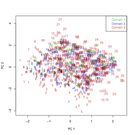
(a) $\gamma_{M}=0$

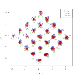
(b) $\gamma_{M}=0.1$

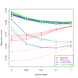
(c) matching errors (weighted)

Figure 5: Experiment 1. (a) and (b) Scatter plots of the first two components of CDMCA with $\gamma_{M}=0$ and $\gamma_{M}=0.1$ respectively. (c) True matching error of $\bm{\bar{W}}_{A}$, and the other matching errors computed from $\bm{W}$.

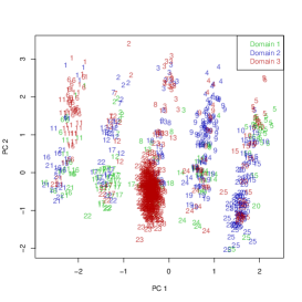
(a) $\gamma_{M}=0$

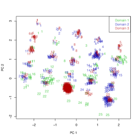
(b) $\gamma_{M}=0.1$

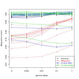
(c) matching errors (unweighted)

Figure 6: Experiment 5. (a) and (b) Scatter plots of the first two components of CDMCA with $\gamma_{M}=0$ and $\gamma_{M}=0.1$ respectively. (c) True matching error of $\bm{\bar{W}}_{B}$, and the other matching errors computed from $\bm{W}$.

$\bm{X}$ is generated by projecting underlying $5\times 5$ grid points in $\mathbb{R}^{2}$ to the higher dimensional spaces for domains with small additive noise. Scatter plots of $\bm{y}^{k}$, $k=1,2$, are shown for Experiments 1 and 5, respectively, in Fig. 5 and Fig. 6. The underlying structure of $5\times 5$ grid points is well observed in the scatter plots for $\gamma_{M}=0.1$, while the structure is obscured in the plots for $\gamma_{M}=0$. For recovering the hidden structure in $\bm{X}$ and $\bm{W}$, the value $\gamma_{M}=0.1$ looks better than $\gamma_{M}=0$.

In Fig. 5(c) and Fig. 6(c), the curves of matching errors are shown for the components $\bm{y}^{k}$, $k=1,\ldots,20$. They are plotted at $\gamma_{M}=0,0.001,0.01,0.1,1$. The smallest two curves ($k=1,2$) are clearly separated from the other 18 curves ($k=3,\ldots,20$), suggesting correctly $K=2$. Looking at the true matching error $\phi_{k}^{\rm true}(\bm{W},\bm{\bar{W}})$, we observe that the true error is minimized at $\gamma_{M}=0.1$ for $k=1,2$. The fitting error $\phi_{k}^{\rm fit}(\bm{W})$, however, underestimates the true error, and wrongly suggests $\gamma_{M}=0$.

For computing the the cv error $\phi_{k}^{\rm cv}(\bm{W})$, we used both the link resampling and the node resampling. These two cv errors accurately estimates the true error in Experiment 1, where each node has very few links in $\bm{W}$. In Experiment 5, some nodes have more links, and only the link resampling estimates the true error very well.

In each of the twelve experiments, we generated 160 datasets of $\bm{W}$. We computed the expected values of the matching errors by taking the simulation average of them. We look at the bias of a matching error divided by its true value. $({E(\phi_{k}^{\rm fit})-E(\phi_{k}^{\rm true})})/{E(\phi_{k}^{\rm true})}$ or $({E(\phi_{k}^{\rm cv})-E(\phi_{k}^{\rm true})})/{E(\phi_{k}^{\rm true})}$ is computed for $k=1,\ldots,10$, with $\gamma_{M}=0.001,0.01,0.1,1$. These $10\times 4=40$ values are used for each boxplot in Fig. 7 and Fig. 8. The two figures correspond to the two types of rescaling factor $b_{k}$, respectively, in Section 3.3. We observe that the fitting error underestimates the true error. The cv error of link resampling is almost unbiased in Experiments 1 to 6, where $\bm{W}$ is generated by link sampling. This verifies our theory of Section 6 to claim that the cv error is asymptotically unbiased for estimating the true error. However, it behaves poorly in Experiments 7 to 12, where $\bm{W}$ is generated by node sampling. On the other hand, the cv error of node resampling performs better than link resampling in Experiments 7 to 12, suggesting appropriate choice of resampling scheme may be important.

The two rescaling factors behave very similarly overall. Comparing Fig. 7 and Fig. 8, we observe that the unweighted variance may lead to more stable results than the weighted variance. This may happen because only a limited number of $y_{1k},\ldots,y_{Nk}$ is used in the weighted variance when $\bm{W}$ is very sparse.

6 Asymptotic theory of the matching errors

6.1 Main results

We investigate the three types of matching errors defined in Section 4. We work on the asymptotic theory for sufficiently large $N$ under the assumptions given below. Some implications of these assumptions are mentioned in Section 6.2.

1. We consider the limit of $N\to\infty$ for asymptotic expansions. $P$ is a constant or increasing as $N\to\infty$, but not too large as $P=o(N^{1/2})$. The sampling scheme is (1), and the resampling scheme is (10). The sampling probability of $\bm{W}$ from $\bm{\bar{W}}$ is $\epsilon=o(1)$ but not too small as $\epsilon^{-1}=o(N)$. The resampling probability of $\bm{W}^{*}$ from $\bm{W}$ is proportional to $N^{-1}$; $\kappa=O(N^{-1})$ and $\kappa^{-1}=O(N)$.

2. The true matching weights are $\bar{w}_{ij}=O(1)$. In general, the asymptotic order of a matrix or a vector is defined as the maximum order of the elements in this paper, so we write $\bm{\bar{W}}=O(1)$. The number of nonzero elements of each row (or each column) is $\#\{\bar{w}_{ij}\neq 0,j=1,\ldots,N\}=O(\epsilon^{-1})$ for $i=1,\ldots,N$.

3. The elements of $\bm{X}$ are $x_{ik}=O(N^{-1/2})$. This is only a technical assumption for the asymptotic argument. In practice, we may assume $x_{ik}=O(1)$ for MCA computation, and redefine $\bm{x}^{k}:=\bm{x}^{k}/\|\bm{x}^{k}\|$ for the theory.

4. Let $\gamma$ be a generic order parameter for representing the magnitude of regularization terms as $\Delta\bm{G}=O(\gamma)$ and $\Delta\bm{H}=O(\gamma)$. For example, we put $\bm{L}_{M}=O(1)$ and $\gamma_{M}=\gamma$. We assume $\gamma=O(N^{-1/2})$.

5. All the $P$ eigenvalues are distinct from the others; $\lambda_{i}\neq\lambda_{j}$ for $i\neq j$. $\bm{A}$ is of full rank, and assume $\bm{A}=O(P^{-1})$. We evaluate $\phi_{k}$ only for $k=1,\ldots,J$, for some $J\leq P$. We assume that $J$ is bounded and $(\lambda_{i}-\lambda_{j})^{-1}=O(1)$ for $i\neq j$ with $i\leq P$, $j\leq J$. These assumptions apply to all the cases under consideration such as $\Delta\bm{G}=\Delta\bm{H}=\bm{0}$ or $\bm{W}$ being replaced by $\epsilon\bm{\bar{W}}$.

Theorem 1.

Under the assumptions mentioned above, the following equation holds.

$$E(\phi_{k}^{\rm fit}(\bm{W})-\phi_{k}^{\rm true}(\bm{W},\bm{\bar{W}}))=(1-\epsilon)E(\phi_{k}^{\rm fit}(\bm{W})-\phi_{k}^{\rm cv}(\bm{W}))+O(N^{-3/2}P^{2}+\gamma^{3}P^{3}).$$ (13)

This implies

$$E(\phi_{k}^{\rm cv}(\bm{W}))=E(\phi_{k}^{\rm true}(\bm{W},\bm{\bar{W}}))+O(\epsilon N^{-1}P+N^{-3/2}P^{2}+\gamma^{3}P^{3}).$$ (14)

Therefore, the cross-validation error is an unbiased estimator of the true error by ignoring the higher-order term of $O(\epsilon N^{-1}P+N^{-3/2}P^{2}+\gamma^{3}P^{3})=o(1)$, which is smaller than $E(\phi_{k}^{\rm cv}(\bm{W}))=O(1)$ for sufficiently large $N$.

Proof.

By comparing (27) of Lemma 3 and (30) of Lemma 4, we obtain (13) immediately. Then (14) follows, because $E(\phi_{k}^{\rm fit}(\bm{W})-\phi_{k}^{\rm true}(\bm{W}))=O(N^{-1}P)$ as mentioned in Lemma 3. ∎

We use $N,P,\gamma,\epsilon$ in expressions of asymptotic orders. Higher order terms can be simplified by substituting $P=o(N^{1/2})$ and $\gamma=O(N^{-1/2})$. For example, $O(N^{-3/2}P^{2}+\gamma^{3}P^{3})=o(N^{-1/2}+1)=o(1)$ in (13). However, we attempt to leave the terms with $P$ and $\gamma$ for finer evaluation.

The theorem justifies the link resampling for estimating the true matching error under the link sampling scheme. Now we have theoretically confirmed our observation that the cross-validation is nearly unbiased in the numerical examples of Sections 2 and 5. Although the fitting error underestimates the true error in the numerical examples, it has not been clear that the bias is negative in some sense from the expression of the bias given in Lemma 3.

In the following subsections, we will discuss lemmas used for the proof of Theorem 1. In Section 6.2, we look at the assumptions of the theorem. In Section 6.3, the solution of the optimization problem and the matching error are expressed in terms of small perturbation of the regularization matrices. Lemma 1 gives the asymptotic expansions of the eigenvalues $\lambda_{1},\ldots,\lambda_{P}$ and the linear transformation matrix $\bm{A}$ in terms of $\Delta\bm{G}$ and $\Delta\bm{H}$. Lemma 2 gives the asymptotic expansion of the matching error $\phi_{k}(\bm{W},\bm{\tilde{W}})$ in terms of $\Delta\bm{G}$ and $\Delta\bm{H}$. Using these results, the bias for estimating the true error is discussed in Section 6.4. Lemma 3 gives the asymptotic expansion of the bias of the fitting error, and Lemma 4 shows that the cross-validation adjusts the bias. All the proofs of lemmas are given in Appendix C.

6.2 Some technical notes

We put $K=P$ for the definitions of matrices in Section 6 without losing generality. For characterizing the solution $\bm{A}\in\mathbb{R}^{P\times P}$ of the optimization problem in Section 3.3, (6) and (8) are now, with $\bm{\Lambda}=\mathop{\rm diag}\nolimits(\lambda_{1},\ldots,\lambda_{P})$,

$$\bm{A}^{T}\bm{G}\bm{A}=\bm{I}_{P},\quad\bm{A}^{T}\bm{H}\bm{A}=\bm{\Lambda}.$$ (15)

We can do so, because the solution $\bm{a}^{k}$ and the eigenvalue $\lambda_{k}$ for the $k$-th component does not change for each $1\leq k\leq K$ when the value of $K$ changes. This property also holds for the matching errors of the $k$-th component. Therefore a result shown for some $1\leq k\leq P$ with $K=P$ holds true for the same $k$ with any $K\leq P$, meaning that we can put $K=P$ in Section 6. In our asymptotic theory, however, we would like to confine $k$ to a finite value. So we restrict our attention to $1\leq k\leq J$ in the assumption (A5).

The assumption of $N$ and $P$ in (A1) covers many applications in practice. The theory may work for the case that $N$ is hundreds and $P$ is dozens, or for a more recent case that $N$ is millions and $P$ is hundreds.

Asymptotic properties of $\bm{W}$ follow from (A1) and (A2). Since the elements of $\bm{W}$ are sampled from $\bm{\bar{W}}$, we have $\bm{W}=O(1)$ and $\bm{M}=O(1)$. The number of nonzero elements for each row (or each column) is

$$\#\{w_{ij}\neq 0,j=1,\ldots,N\}=O(1),\quad i=1,\ldots,N,$$ (16)

and the total number of nonzero elements is $\#\{w_{ij}\neq 0,i,j=1,\ldots,N\}=O(N)$. Thus $\bm{W}$ is assumed to be a very sparse matrix. Examples of such sparse matrices are image-tag links in Flickr, or more typically friend links in Facebook. Although the label domains of MNIST dataset do not satisfy (16) with many links to images, our method still worked very well.

The assumption of $\kappa$ in (A1) implies that the number of nonzero elements in $\bm{W}^{*}$ is $O(1)$. Similarly to the leave-one-out cross-validation of data vectors, we resample very few links in our cross-validation.

From (A3), $\sum_{i=1}^{N}m_{i}x_{ik}x_{jl}=O(N(N^{-1/2})^{2})=O(1)$, and thus $\bm{X}^{T}\bm{M}\bm{X}=O(1)$, and $\bm{G}=O(1)$. Also, $\sum_{i=1}^{N}\sum_{j=1}^{N}w_{ij}x_{ik}x_{jl}=\sum_{(i,j):w_{ij}\neq 0}w_{ij}x_{ik}x_{jl}=O(N(N^{-1/2})^{2})=O(1)$, and thus $\bm{X}^{T}\bm{W}\bm{X}=O(1)$, and $\bm{H}=O(1)$. From (A5), $\sum_{i=1}^{P}\sum_{j=1}^{P}(\bm{G})_{ij}a_{ik}a_{jk}=O(P^{2}(P^{-1})^{2})=O(1)$, which is necessary for $\bm{A}^{T}\bm{G}\bm{A}=\bm{I}_{P}$. Then $\bm{Y}=\bm{X}\bm{A}=O(PN^{-1/2}P^{-1})=O(N^{-1/2})$.

The assumptions on the eigenvalues described in (A5) may be difficult to hold in practice. In fact, there are many zero eigenvalues in the examples of Section 5; 60 zeros, 40 positives ($K^{+}=40$), and 40 negatives in the $P=140$ eigenvalues. Looking at Experiment 1, however, we observed that $\phi_{k}^{\rm cv}\approx\phi_{k}^{\rm true}$ holds well and $E(\phi_{k}^{\rm cv})=E(\phi_{k}^{\rm true})$ holds very accurately for $k=1,\ldots,40$ ($\lambda_{k}>0$) when $\gamma_{M}>0$. The eigenvalues for $\gamma_{M}=0.1$ are $\lambda_{1}=0.988,\lambda_{2}=0.978,\lambda_{3}=0.562,\lambda_{4}=0.509,\lambda_{5}=0.502,\ldots$, where $\lambda_{1}-\lambda_{2}$ looks very small, but it did not cause any problem. On the other hand, the eigenvalues for $\gamma_{M}=0$ are $\lambda_{1}=0.999,\lambda_{2}=0.997,\lambda_{3}=0.973,\lambda_{4}=0.971,\lambda_{5}=0.960,\ldots$, where some $\lambda_{k}$ are very close to each other. This might be a cause for the deviation of $\phi_{k}^{\rm cv}$ from $\phi_{k}^{\rm true}$ when $\gamma_{M}=0$.

6.3 Small change in $\bm{A}$, $\bm{\Lambda}$, and the matching error

Here we show how $\bm{A}$, $\bm{\Lambda}$ and $\phi_{k}(\bm{W},\bm{\tilde{W}})$ depend on $\Delta\bm{G}$ and $\Delta\bm{H}$. Recall that terms with hat are for $\Delta\bm{G}=\Delta\bm{H}=\bm{0}$ as defined in Section 3.2; $\bm{\hat{G}}=\bm{X}^{T}\bm{M}\bm{X}$, $\bm{\hat{H}}=\bm{X}^{T}\bm{W}\bm{X}$, $\bm{\hat{Y}}=\bm{X}\bm{\hat{A}}$. The optimization problem is characterized as $\bm{\hat{A}}^{T}\bm{\hat{G}}\bm{\hat{A}}=\bm{I}_{P}$, $\bm{\hat{A}}^{T}\bm{\hat{H}}\bm{\hat{A}}=\bm{\hat{\Lambda}}$, where $\bm{\hat{\Lambda}}=\mathop{\rm diag}\nolimits(\hat{\lambda}_{1},\ldots,\hat{\lambda}_{P})$ is the diagonal matrix of the eigenvalues $\hat{\lambda}_{1},\ldots,\hat{\lambda}_{P}$. Then $\bm{A}$ and $\bm{\Lambda}$ are defined in Section 3.3 for $\bm{G}=\bm{\hat{G}}+\Delta\bm{G}$ and $\bm{H}=\bm{\hat{H}}+\Delta\bm{H}$. They satisfy (15). The asymptotic expansions for $\bm{A}$ and $\bm{\Lambda}$ will be given in Lemma 1 using

$$\bm{g}=\bm{\hat{A}}^{T}\Delta\bm{G}\bm{\hat{A}},\quad\bm{h}=\bm{\hat{A}}^{T}\Delta\bm{H}\bm{\hat{A}}\in\mathbb{R}^{P\times P}.$$

For proving the lemma in Section C.1, we will solve (15) under the small perturbation of $\bm{g}$ and $\bm{h}$.

Lemma 1.

Let $\Delta\bm{\Lambda}=\bm{\Lambda}-\bm{\hat{\Lambda}}$ with elements $\Delta\lambda_{i}=\lambda_{i}-\hat{\lambda}_{i}$, $i=1,\ldots,P$. Define $\bm{C}\in\mathbb{R}^{P\times P}$ as $\bm{C}=\bm{\hat{A}}^{-1}\bm{A}-\bm{I}_{P}$ so that $\bm{A}=\bm{\hat{A}}(\bm{I}_{P}+\bm{C})$. Here $\bm{\hat{A}}^{-1}$ exists, since we assumed that $\bm{\hat{A}}$ is of full rank in (A5). We assume $\bm{g}=O(\gamma)$ and $\bm{h}=O(\gamma)$.

Then the elements of $\Delta\bm{\Lambda}=O(\gamma)$ are, for $i=1,\ldots,P$,

$$\Delta\lambda_{i}=-(g_{ii}\hat{\lambda}_{i}-h_{ii})+\delta\lambda_{i}$$ (17)

with $\delta\lambda_{i}=O(\gamma^{2}P)$ defined for $i\leq J$ as

$$\delta\lambda_{i}=g_{ii}(g_{ii}\hat{\lambda}_{i}-h_{ii})-\sum_{j\neq i}(\hat{\lambda}_{j}-\hat{\lambda}_{i})^{-1}(g_{ij}\hat{\lambda}_{i}-h_{ij})^{2}+O(\gamma^{3}P^{2}),$$ (18)

where $\sum_{j\neq i}$ is the summation over $j=1,\ldots,P$, except for $j=i$.

The elements of the diagonal part of $\bm{C}=O(\gamma)$ are, for $i=1,\ldots,P$,

$$c_{ii}=-\frac{1}{2}g_{ii}+\delta c_{ii}$$ (19)

with $\delta c_{ii}=O(\gamma^{2}P)$ defined for $i\leq J$ as

$$\delta c_{ii}=\frac{3}{8}(g_{ii})^{2}-\sum_{j\neq i}(\hat{\lambda}_{j}-\hat{\lambda}_{i})^{-2}(g_{ij}\hat{\lambda}_{i}-h_{ij})\Bigl{\{}g_{ij}\Bigl{(}\hat{\lambda}_{j}-\frac{1}{2}\hat{\lambda}_{i}\Bigr{)}-\frac{1}{2}h_{ij}\Bigr{\}}+O(\gamma^{3}P^{2}),$$ (20)

and the elements of the off-diagonal ($i\neq j$) part of $\bm{C}$ are, for either $i\leq J,j\leq P$ or $i\leq P,j\leq J$, i.e., one of $i$ and $j$ is not greater than $J$,

$$c_{ij}=(\hat{\lambda}_{i}-\hat{\lambda}_{j})^{-1}(g_{ij}\hat{\lambda}_{j}-h_{ij})+\delta c_{ij}$$ (21)

with $\delta c_{ij}=O(\gamma^{2}P)$ defined for $i\leq P,j\leq J$ as

$$\begin{split}\delta c_{ij}=&-\frac{1}{2}(\hat{\lambda}_{i}-\hat{\lambda}_{j})^{-1}(g_{ij}\hat{\lambda}_{j}-h_{ij})g_{jj}-(\hat{\lambda}_{i}-\hat{\lambda}_{j})^{-2}(g_{ij}\hat{\lambda}_{i}-h_{ij})(g_{jj}\hat{\lambda}_{j}-h_{jj})\\ &+(\hat{\lambda}_{i}-\hat{\lambda}_{j})^{-1}\sum_{k\neq j}(\hat{\lambda}_{k}-\hat{\lambda}_{j})^{-1}(g_{ki}\hat{\lambda}_{j}-h_{ki})(g_{kj}\hat{\lambda}_{j}-h_{kj}).\end{split}$$ (22)

The asymptotic expansion of $\phi_{k}(\bm{W},\bm{\tilde{W}})$ is given in Lemma 2. For proving the lemma in Section C.2, the matching error is first expressed by $\bm{C}$, and then the result of Lemma 1 is used for simplifying the expression.

Lemma 2.

Let $\bm{\tilde{S}}=\bm{\hat{A}}^{T}\bm{X}^{T}(\bm{\tilde{M}}-\bm{\tilde{W}})\bm{X}\bm{\hat{A}}=\bm{\hat{Y}}^{T}(\bm{\tilde{M}}-\bm{\tilde{W}})\bm{\hat{Y}}\in\mathbb{R}^{P\times P}$. We assume $\bm{\tilde{S}}=O(1)$, which holds for, say, $\bm{\tilde{W}}=\bm{W}$ and $\bm{\tilde{W}}=\epsilon\bm{\bar{W}}$. We assume $\bm{g}=O(\gamma)$ and $\bm{h}=O(\gamma)$. Then the matching error of Section 3.1 is expressed asymptotically as

$$\begin{split}\phi_{k}(\bm{W},&\bm{\tilde{W}})=\tilde{s}_{kk}+\sum_{i\neq k}2(\hat{\lambda}_{i}-\hat{\lambda}_{k})^{-1}\tilde{s}_{ik}(g_{ik}\hat{\lambda}_{k}-h_{ik})\\ &-\sum_{i\neq k}(\hat{\lambda}_{i}-\hat{\lambda}_{k})^{-2}\Bigl{\{}\tilde{s}_{kk}(g_{ik}\hat{\lambda}_{k}-h_{ik})^{2}+\tilde{s}_{ik}(g_{ki}\hat{\lambda}_{i}-h_{ki})(g_{kk}\hat{\lambda}_{k}-h_{kk})\Bigr{\}}\\ &+\sum_{i\neq k}\sum_{j\neq k}(\hat{\lambda}_{i}-\hat{\lambda}_{k})^{-1}(\hat{\lambda}_{j}-\hat{\lambda}_{k})^{-1}\Bigr{\{}2\tilde{s}_{ik}(g_{ij}\hat{\lambda}_{k}-h_{ij})(g_{jk}\hat{\lambda}_{k}-h_{jk})\\ &\hskip 100.00015pt+\tilde{s}_{ij}(g_{ik}\hat{\lambda}_{k}-h_{ik})(g_{jk}\hat{\lambda}_{k}-h_{jk})\Bigr{\}}+O(\gamma^{3}P^{3}).\end{split}$$ (23)

Let us further assume $\bm{\tilde{W}}=\bm{W}$. Then $\bm{\tilde{S}}=\bm{I}_{P}-\bm{\hat{\Lambda}}$ with elements $\tilde{s}_{ij}=\delta_{ij}(1-\hat{\lambda}_{i})$. Substituting it into (23), we get an expression of $\phi_{k}^{\rm fit}(\bm{W})=\phi_{k}(\bm{W},\bm{W})$ as

$$\phi_{k}^{\rm fit}(\bm{W})=1-\hat{\lambda}_{k}-\sum_{i\neq k}(\hat{\lambda}_{i}-\hat{\lambda}_{k})^{-1}(g_{ik}\hat{\lambda}_{k}-h_{ik})^{2}+O(\gamma^{3}P^{3}).$$ (24)

It follows from (A4) and (A5) that the magnitude of the regularization terms are expressed as $\bm{g}=O(\gamma)$ and $\bm{h}=O(\gamma)$. This is mentioned as an assumption in Lemma 1 and Lemma 2 for the sake of clarity. Although these two lemmas are shown for the regularization terms, they hold generally for any small perturbation other than the regularization terms. Later, in the proofs of Lemma 3 and Lemma 4, we will apply Lemma 1 and Lemma 2 to perturbation of other types with $\gamma=O(N^{-1/2})$ or $\gamma=O(N^{-1})$.

6.4 Bias of the fitting error

Let us consider the optimization problem with respect to $\epsilon\bm{\bar{W}}$. We define $\bm{\bar{A}}$ and $\bm{\bar{\Lambda}}$ as the solution of $\bm{\bar{A}}^{T}\bm{\bar{G}}\bm{\bar{A}}=\bm{I}_{P}$ and $\bm{\bar{A}}^{T}\bm{\bar{H}}\bm{\bar{A}}=\bm{\bar{\Lambda}}$ with $\bm{\bar{G}}=\epsilon\bm{X}^{T}\bm{\bar{M}}\bm{X}$ and $\bm{\bar{H}}=\epsilon\bm{X}^{T}\bm{\bar{W}}\bm{X}$. The eigenvalues are $\bar{\lambda}_{1},\ldots,\bar{\lambda}_{P}$ and the matrix is $\bm{\bar{\Lambda}}=\mathop{\rm diag}\nolimits(\bar{\lambda}_{1},\ldots,\bar{\lambda}_{P})$. We also define $\bm{\bar{Y}}=\bm{X}\bm{\bar{A}}$. These quantities correspond to those with hat, but $\bm{W}$ is replaced by $\epsilon\bm{\bar{W}}$. We then define matrices representing change from $\epsilon\bm{\bar{W}}$ to $\bm{W}$: $\Delta\bm{\hat{W}}=\bm{W}-\epsilon\bm{\bar{W}}$, $\Delta\bm{\hat{M}}=\bm{M}-\epsilon\bm{\bar{M}}$, $\Delta\bm{\hat{G}}=\bm{X}^{T}\Delta\bm{\hat{M}}\bm{X}$ and $\Delta\bm{\hat{H}}=\bm{X}^{T}\Delta\bm{\hat{W}}\bm{X}$.

In Section 6.3, $\bm{g}$ and $\bm{h}$ are used for describing change with respect to the regularization terms $\Delta\bm{G}$ and $\Delta\bm{H}$. Quite similarly,

$$\bm{\hat{g}}=\bm{\bar{A}}^{T}\Delta\bm{\hat{G}}\bm{\bar{A}}=\bm{\bar{Y}}^{T}\Delta\bm{\hat{M}}\bm{\bar{Y}},\quad\bm{\hat{h}}=\bm{\bar{A}}^{T}\Delta\bm{\hat{H}}\bm{\bar{A}}=\bm{\bar{Y}}^{T}\Delta\bm{\hat{W}}\bm{\bar{Y}}$$

will be used for describing change with respect to $\Delta\bm{\hat{G}}$ and $\Delta\bm{\hat{H}}$, namely, change from $\epsilon\bm{\bar{W}}$ to $\bm{W}$. The elements of $\bm{\hat{g}}=(\hat{g}_{ij})$ and $\bm{\hat{h}}=(\hat{h}_{ij})$ are

$$\begin{split}\hat{g}_{ij}&=(\bm{\bar{y}}^{i})^{T}\Delta\bm{\hat{M}}\bm{\bar{y}}^{j}=\sum_{l>m}(\bar{y}_{li}\bar{y}_{lj}+\bar{y}_{mi}\bar{y}_{mj})\Delta\hat{w}_{lm}+\sum_{l=1}^{N}y_{li}y_{lj}\Delta\hat{w}_{ll},\\ \hat{h}_{ij}&=(\bm{\bar{y}}^{i})^{T}\Delta\bm{\hat{W}}\bm{\bar{y}}^{j}=\sum_{l>m}(\bar{y}_{li}\bar{y}_{mj}+\bar{y}_{mi}\bar{y}_{lj})\Delta\hat{w}_{lm}+\sum_{l=1}^{N}y_{li}y_{lj}\Delta\hat{w}_{ll},\end{split}$$

and they will be denoted as

$$\hat{g}_{ij}=\sum_{l\geq m}{\cal G}[\bm{\bar{Y}}]_{lm}^{ij}\Delta\hat{w}_{lm},\quad\hat{h}_{ij}=\sum_{l\geq m}{\cal H}[\bm{\bar{Y}}]_{lm}^{ij}\Delta\hat{w}_{lm},$$ (25)

where $\sum_{l>m}=\sum_{l=2}^{N}\sum_{m=1}^{l-1}$ and $\sum_{l\geq m}=\sum_{l=1}^{N}\sum_{m=1}^{l}$.

We are now ready to consider the bias of the fitting error. The difference of the fitting error from the true error is

$$\phi_{k}^{\rm fit}(\bm{W})-\phi_{k}^{\rm true}(\bm{W},\bm{\bar{W}})=\phi_{k}(\bm{W},\Delta\bm{\hat{W}}).$$ (26)

The asymptotic expansion of (26) is given by Lemma 2 with $\bm{\tilde{W}}=\Delta\bm{\hat{W}}$. This expression will be rewritten by $\bm{\hat{g}}$ and $\bm{\hat{h}}$ in Section C.3 for proving the following lemma. For rewriting $\bm{\hat{A}}$ and $\bm{\hat{\Lambda}}$ in terms of $\bm{\bar{A}}$ and $\bm{\bar{\Lambda}}$, Lemma 1 will be used there.

Lemma 3.

Bias of the fitting error for estimating the true error is expressed asymptotically as

$$E(\phi_{k}^{\rm fit}(\bm{W})-\phi_{k}^{\rm true}(\bm{W},\bm{\bar{W}}))={\rm bias}_{k}+O(N^{-3/2}P^{2}+\gamma^{3}P^{3}),$$ (27)

where ${\rm bias}_{k}=O(N^{-1}P)$ is defined as

$${\rm bias}_{k}=E\Bigl{[}-(\hat{g}_{kk}-\hat{h}_{kk})\hat{g}_{kk}+\sum_{j\neq k}2(\bar{\lambda}_{j}-\bar{\lambda}_{k})^{-1}(\hat{g}_{jk}-\hat{h}_{jk})(\hat{g}_{jk}\bar{\lambda}_{k}-\hat{h}_{jk})\Bigr{]}$$

using the elements of $\bm{\hat{g}}$, $\bm{\hat{h}}$ and $\bm{\bar{\Lambda}}$ mentioned above. ${\rm bias}_{k}$ can be expressed as

$$\begin{split}{\rm bias}_{k}=\epsilon(1-\epsilon)\sum_{l\geq m}\bar{w}_{lm}^{2}\Bigl{[}&-({\cal G}[\bm{\bar{Y}}]_{lm}^{kk}-{\cal H}[\bm{\bar{Y}}]_{lm}^{kk}){\cal G}[\bm{\bar{Y}}]_{lm}^{kk}\\ &+\sum_{j\neq k}2(\bar{\lambda}_{j}-\bar{\lambda}_{k})^{-1}({\cal G}[\bm{\bar{Y}}]_{lm}^{jk}-{\cal H}[\bm{\bar{Y}}]_{lm}^{jk})({\cal G}[\bm{\bar{Y}}]_{lm}^{jk}\bar{\lambda}_{k}-{\cal H}[\bm{\bar{Y}}]_{lm}^{jk})\Bigr{]}.\end{split}$$ (28)

We also have $\bm{\hat{g}}=O(N^{-1/2})$ and $\bm{\hat{h}}=O(N^{-1/2})$.

In the following lemma, we will show that the bias of the fitting error is adjusted by the cross-validation. For proving the lemma in Section C.4, we will first give the asymptotic expansion of $\phi_{k}((1-\kappa)^{-1}(\bm{W}-\bm{W^{*}}),\kappa^{-1}\bm{W}^{*})$ using Lemma 2. The expression will be rewritten using the change from $\bm{\hat{A}}$ and $\bm{\hat{\Lambda}}$ to those with respect to $(1-\kappa)^{-1}(\bm{W}-\bm{W^{*}})$. The asymptotic expansion of $\phi_{k}^{\rm cv}$ will be obtained by taking the expectation with respect to (10). Finally, we will take the expectation with respect to (1).

Lemma 4.

The difference of the fitting error from the cross-validation error is expressed asymptotically as

$$\begin{split}\phi_{k}^{\rm fit}(\bm{W})-&\phi_{k}^{\rm cv}(\bm{W})=\sum_{l\geq m}w_{lm}^{2}\Bigl{[}-({\cal G}[\bm{\hat{Y}}]_{lm}^{kk}-{\cal H}[\bm{\hat{Y}}]_{lm}^{kk}){\cal G}[\bm{\hat{Y}}]_{lm}^{kk}\\ &+\sum_{j\neq k}2(\hat{\lambda}_{j}-\hat{\lambda}_{k})^{-1}({\cal G}[\bm{\hat{Y}}]_{lm}^{jk}-{\cal H}[\bm{\hat{Y}}]_{lm}^{jk})({\cal G}[\bm{\hat{Y}}]_{lm}^{jk}\hat{\lambda}_{k}-{\cal H}[\bm{\hat{Y}}]_{lm}^{jk})\Bigr{]}\\ &\qquad+O(N^{-2}P^{2}+N^{-1}\gamma P^{2}+\gamma^{3}P^{3}),\end{split}$$ (29)

and its expected value is

$$E(\phi_{k}^{\rm fit}(\bm{W})-\phi_{k}^{\rm cv}(\bm{W}))=(1-\epsilon)^{-1}{\rm bias}_{k}+O(N^{-3/2}P^{2}+\gamma^{3}P^{3}).$$ (30)

Appendix A Cross-domain matching correlation analysis

A.1 A simple coding for cross-domain matching

Here we explain how CDMCA is converted to MCA. Let $\bm{x}^{(d)}_{i}\in\mathbb{R}^{p_{d}}$, $i=1,\ldots,n_{d}$, denote the data vectors of domain $d$. Each $\bm{x}^{(d)}_{i}$ is coded as an augmented vector $\bm{\tilde{x}}^{(d)}_{i}\in\mathbb{R}^{P}$ defined as

$$(\bm{\tilde{x}}^{(d)}_{i})^{T}=\Bigl{(}(\bm{0}_{p_{1}})^{T},\ldots,(\bm{0}_{p_{d-1}})^{T},(\bm{x}^{(d)}_{i})^{T},(\bm{0}_{p_{d+1}})^{T},\ldots,(\bm{0}_{p_{D}})^{T}\Bigr{)}.$$ (31)

Here, $\bm{0}_{p}\in\mathbb{R}^{p}$ is the vector with zero elements. This is a sparse coding (Olshausen and Field, 2004) in the sense that nonzero elements for domains do not overlap each other. All the $N$ vectors of $D$ domains are now represented as points in the same $\mathbb{R}^{P}$. We take these $N$ vectors as $\bm{x}_{i}\in\mathbb{R}^{P}$, $i=1,\ldots,N$. Then CDMCA reduces to MCA. The data matrix is expressed as

$$\bm{X}^{T}=(\bm{\tilde{x}}^{(1)}_{1},\ldots,\bm{\tilde{x}}^{(1)}_{n_{1}},\ldots,\bm{\tilde{x}}^{(D)}_{1},\ldots,\bm{\tilde{x}}^{(D)}_{n_{D}}).$$

Let $\bm{X}^{(d)}\in\mathbb{R}^{n_{d}\times p_{d}}$ be the data matrix of domain $d$ defined as $(\bm{X}^{(d)})^{T}=(\bm{x}^{(d)}_{1},\ldots,\bm{x}^{(d)}_{n_{d}})$. The data matrix of the augmented vectors is now expressed as $\bm{X}=\mathop{\rm Diag}\nolimits(\bm{X}^{(1)},\ldots,\bm{X}^{(D)})$, where $\mathop{\rm Diag}\nolimits()$ indicates a block diagonal matrix.

Let us consider partitions of $\bm{A}$ and $\bm{Y}$ as $\bm{A}^{T}=((\bm{A}^{(1)})^{T},\ldots,(\bm{A}^{(D)})^{T})$ and $\bm{Y}^{T}=((\bm{Y}^{(1)})^{T},\ldots,(\bm{Y}^{(D)})^{T})$ with $\bm{A}^{(d)}\in\mathbb{R}^{p_{d}\times K}$ and $\bm{Y}^{(d)}\in\mathbb{R}^{n_{d}\times K}$. Then the linear transformation of MCA, $\bm{Y}=\bm{X}\bm{A}$, is expressed as

$$\bm{Y}^{(d)}=\bm{X}^{(d)}\bm{A}^{(d)},\quad d=1,\ldots,D,$$

which are the linear transformations of CDMCA. The matching weight matrix between domains $d$ and $e$ is $\bm{W}^{(de)}=(w^{(de)}_{ij})\in\mathbb{R}^{n_{d}\times n_{e}}$ for $d,e=1,\ldots,D$. They are placed in a array to define $\bm{W}=(\bm{W}^{(de)})\in\mathbb{R}^{N\times N}$. Then the matching error of MCA is expressed as

$$\phi=\frac{1}{2}\sum_{d=1}^{D}\sum_{e=1}^{D}\sum_{i=1}^{n_{d}}\sum_{j=1}^{n_{e}}w^{(de)}_{ij}\|\bm{y}^{(d)}_{i}-\bm{y}^{(e)}_{j}\|^{2},$$

which is the matching error of CDMCA.

Notice $\bm{M}=\mathop{\rm Diag}\nolimits(\bm{M}^{(1)},\ldots,\bm{M}^{(D)})$ with $\bm{M}^{(d)}=\mathop{\rm diag}\nolimits((\bm{W}^{(d1)},\ldots,\bm{W}^{(dD)})\bm{1}_{N})$, and so $\bm{X}^{T}\bm{M}\bm{X}=\mathop{\rm Diag}\nolimits((\bm{X}^{(1)})^{T}\bm{M}^{(1)}\bm{X}^{(1)},\ldots,(\bm{X}^{(D)})^{T}\bm{M}^{(D)}\bm{X}^{(D)})$ is computed efficiently by looking at only the block diagonal parts.

Let us consider a simple case with $n_{1}=\cdots=n_{D}=n$, $N=nD$, $\bm{W}^{(de)}=c_{de}\bm{I}_{n}$ using a coefficient $c_{de}\geq 0$ for all $d,e=1,\ldots,D$. Then CDMCA reduces to a version of MCCA, where associations between sets of variables are specified by the coefficients $c_{de}$ (Tenenhaus and Tenenhaus, 2011). Another version of MCCA with all $c_{de}=1$ for $d\neq e$ is discussed extensively in Takane, Hwang and Abdi (2008). For the simplest case of $D=2$ with $c_{12}=1$, $c_{11}=c_{22}=0$, CDMCA reduces to CCA with $\bm{W}=\bigl{(}\begin{smallmatrix}\bm{0}&\bm{I}_{n}\\ \bm{I}_{n}&\bm{0}\end{smallmatrix}\bigr{)}$.

A.2 auto-associative correlation matrix memory

Let us consider $\bm{\Omega}\in\mathbb{R}^{P\times P}$ defined by

$$\bm{\Omega}=\frac{1}{2}\sum_{i=1}^{N}\sum_{j=1}^{N}w_{ij}(\bm{x}_{i}+\bm{x}_{j})(\bm{x}_{i}+\bm{x}_{j})^{T}.$$

This is the correlation matrix of $\bm{x}_{i}+\bm{x}_{j}$ weighted by $w_{ij}$. Since $\bm{\Omega}=\bm{X}^{T}\bm{M}\bm{X}+\bm{X}^{T}\bm{W}\bm{X}$, we have $\bm{\Omega}+\Delta\bm{G}+\Delta\bm{H}=\bm{G}+\bm{H}$, and then MCA of Section 3.3 is equivalent to maximizing $\mathop{\rm tr}\nolimits(\bm{A}^{T}(\bm{\Omega}+\Delta\bm{G}+\Delta\bm{H})\bm{A})$ with respect to $\bm{A}\in\mathbb{R}^{P\times K}$ subject to (6). The role of $\bm{H}$ is now replaced by $\bm{\Omega}+\Delta\bm{G}+\Delta\bm{H}$. Thus MCA is interpreted as dimensionality reduction of the correlation matrix $\bm{\Omega}$ with regularization term $\Delta\bm{G}+\Delta\bm{H}$.

For CDMCA, the correlation matrix becomes

$$\bm{\Omega}=\frac{1}{2}\sum_{d=1}^{D}\sum_{e=1}^{D}\sum_{i=1}^{n_{d}}\sum_{j=1}^{n_{e}}w_{ij}^{(de)}(\bm{\tilde{x}}_{i}^{(d)}+\bm{\tilde{x}}_{j}^{(e)})(\bm{\tilde{x}}_{i}^{(d)}+\bm{\tilde{x}}_{j}^{(e)})^{T}.$$

This is the correlation matrix of the input pattern of a pair of data vectors

$$(\bm{\tilde{x}}^{(d)}_{i}+\bm{\tilde{x}}^{(e)}_{j})^{T}=\Bigl{(}0,\ldots,0,(\bm{x}^{(d)}_{i})^{T},0,\ldots,0,(\bm{x}^{(e)}_{j})^{T},0,\ldots,0\Bigr{)}$$ (32)

weighted by $w_{ij}^{(de)}$. Interestingly, the same correlation matrix is found in one of the classical neural network models. Any part of the memorized vector can be used as a key for recalling the whole vector in the auto-associative correlation matrix memory (Kohonen, 1972), also known as Associatron (Nakano, 1972). This associative memory may recall $\bm{\tilde{x}}^{(d)}_{i}+\bm{\tilde{x}}^{(e)}_{j}$ for input key either $\bm{\tilde{x}}^{(d)}_{i}$ or $\bm{\tilde{x}}^{(e)}_{j}$ if $w_{ij}^{(de)}>0$. In particular, the representation (32) of a pair of data vectors is equivalent to eq. (14) of Nakano (1972). Thus CDMCA is interpreted as dimensionality reduction of the auto-associative correlation matrix memory for pairs of data vectors.

Appendix B Experimental details

B.1 MNIST handwritten digits

The MNIST database of handwritten digits (LeCun et al., 1998) has a training set of 60,000 images, and a test set of 10,000 images. Each image has $28\times 28=784$ pixels of 256 gray levels. We prepared a dataset of cross-domain matching with three domains for illustration purpose.

The data matrix $\bm{X}$ is specified as follows. The first domain ($d=1$) is for the handwritten digit images of $n_{1}=60,000$. Each image is coded as a vector of $p_{1}=2784$ dimensions by concatenating an extra 2000 dimensional vector. We have chosen randomly 2000 pairs of pixels x[i,j], x[k,l] with $|\text{\tt i}-\text{\tt k}|\leq 5$, $|\text{\tt j}-\text{\tt l}|\leq 5$ in advance, and compute the product x[i,j] * x[k,l] for each image. The second domain ($d=2$) is for digit labels of $n_{2}=10$. They are zero, one, two, …, nine. Each label is coded as a random vector of $p_{2}=100$ dimensions with each element generated independently from the standard normal distribution $N(0,1)$. The third domain ($d=3$) is for attribute labels even, odd, and prime ($n_{3}=3$). Each label is coded as a random vector of $p_{3}=50$ dimensions with each element generated independently from $N(0,1)$. The total number of vectors is $N=n_{1}+n_{2}+n_{3}=60013$, and the dimension of the augmented vector is $P=p_{1}+p_{2}+p_{3}=2934$.

The true matching weight matrix $\bm{\bar{W}}$ is specified as follows. The cross-domain matching weight $\bm{\bar{W}}^{(12)}\in\mathbb{R}^{n_{1}\times n_{2}}$ between domain-1 and domain-2 is the 1-of-$K$ coding; $\bar{w}^{(12)}_{ij}=1$ if $i$-th image has $j$-th label, and $\bar{w}^{(12)}_{ij}=0$ otherwise. $\bm{\bar{W}}^{(13)}\in\mathbb{R}^{n_{1}\times n_{3}}$ is defined similarly, but images may have two attribute labels such as an image of 3 has labels odd and prime. We set all elements of $\bm{\bar{W}}^{(23)}$ as zeros, pretending ignorance about the number properties. We then prepared $\bm{W}$ by randomly sampling elements from $\bm{\bar{W}}$ with $\epsilon=0.2$. Only the upper triangular parts of the weight matrices are stored in memory, so that the symmetry $\bm{W}=\bm{W}^{T}$ is automatically hold. The number of nonzero elements in the upper triangular part of the matrix is 143775 for $\bm{\bar{W}}$, and it becomes 28779 for $\bm{W}$. In particular, the number of nonzero elements in $\bm{W}^{(12)}$ is 12057.

The optimal $\bm{A}$ is computed by the method of Section 3.3. The regularization matrix is block diagonal $\bm{L}_{M}=\mathop{\rm Diag}\nolimits(\bm{L}_{M}^{(1)},\bm{L}_{M}^{(2)},\bm{L}_{M}^{(3)})$ with $\bm{L}_{M}^{(d)}=\alpha_{d}\bm{I}_{p_{d}}$ and $\alpha_{d}=\mathop{\rm tr}\nolimits((\bm{X}^{(d)})^{T}\bm{M}^{(d)}\bm{X}^{(d)})/p_{d}$. The regularization parameters are $\gamma_{M}>0$ and $\gamma_{W}=0$. The computation with $\gamma_{M}=0$ actually uses a small value $\gamma_{M}=10^{-6}$. The number of positive eigenvalues is $K^{+}=11$. The appropriate value $K=9$ was chosen by looking at the distribution of eigenvalues $\lambda_{k}$ and $\phi_{k}^{\rm cv}$.

The three types of matching errors of Section 4 are computed as follows. The plotted values are not the component-wise matching errors $\phi_{k}$, but the sum $\phi=\sum_{k=1}^{K}\phi_{k}$. The true matching error $\phi_{k}^{\rm true}(\bm{W},\bm{\bar{W}})$ is computed with $\bm{\bar{W}}$ of the test dataset here, while $\bm{A}$ is computed from the training dataset. This is different from the definition in Section 4.1 but more appropriate if test datasets are available. The fitting error $\phi_{k}^{\rm fit}(\bm{W})$ and the cross-validation error $\phi_{k}^{\rm cv}(\bm{W})$ are computed from the training dataset. In particular, $\phi_{k}^{\rm cv}(\bm{W})$ is computed by resampling elements from $\bm{W}$ with $\kappa=0.1$ so that the number of nonzero elements in the upper triangular part of $\bm{W}^{*}$ is about 3000.

B.2 Simulation datasets

We generated simulation datasets of cross-domain matching with $D=3$, $p_{1}=10,p_{2}=30,p_{3}=100$, $n_{1}=125,n_{2}=250,n_{3}=500$. The two true matching weights $\bm{\bar{W}}_{A}$ and $\bm{\bar{W}}_{B}$ were created at first, and they were unchanged during the experiments. In each of the twelve experiments, $\bm{X}$ and $\bm{W}$ are generated from either of $\bm{\bar{W}}_{A}$ and $\bm{\bar{W}}_{B}$, and then $\bm{W}$ is generated independently 160 times, while $\bm{X}$ is fixed, for taking the simulation average. Computation of the optimal $\bm{A}$ is the same as Appendix B.1 using the same regularization term specified there.

The data matrix $\bm{X}$ is specified as follows. First, 25 points on $5\times 5$ grid in $\mathbb{R}^{2}$ are placed as $(1,1),(1,2),(1,3),(1,4),(1,5),(2,1),\ldots,(5,5)$. They are $(\bm{x}^{(0)}_{1})^{T},\ldots,(\bm{x}^{(0)}_{25})^{T}$, where $d=0$ is treated as a special domain for data generation. Matrices $\bm{B}^{(d)}\in\mathbb{R}^{p_{d}\times 2}$, $d=1,2,3$, are prepared with all elements distributed as $N(0,1)$ independently. Let $n_{d,i}$ be the number of vectors in domain-$d$ generated from $i$-th grid point for $d=1,2,3$, $i=1,\ldots,25$, which will be specified later with constraints $\sum_{i=1}^{25}n_{d,i}=n_{d}$. Then data vectors $\{\bm{x}_{i}^{(d)},i=1,\ldots,n_{d}\}$ are generated as $\bm{x}_{i,j}^{(d)}=\bm{B}^{(d)}\bm{x}^{(0)}_{i}+\bm{\epsilon}^{(d)}_{i,j}$, $i=1,\ldots,25$, $j=1,\ldots,n_{d,i}$, with elements of $\bm{\epsilon}^{(d)}_{i,j}$ distributed as $N(0,0.5^{2})$ independently. Each column of $\bm{X}^{(d)}$ is then standardized to mean zero and variance one.

The true matching weight matrix $\bm{\bar{W}}$ is specified as follows. Two data vectors in different domains $d$ and $e$ are linked to each other as $\bar{w}_{ij}^{(de)}=1$ if they are generated from the same grid point. All other elements in $\bm{\bar{W}}$ are zero. Two types of $\bm{\bar{W}}$, denoted as $\bm{\bar{W}}_{A}$ and $\bm{\bar{W}}_{B}$, are considered. For $\bm{\bar{W}}_{A}$, the numbers of data vectors are the same for all grid points; $n_{1,i}=5$, $n_{2,i}=10$, $n_{3,i}=20$, $i=1,\ldots,25$. For $\bm{\bar{W}}_{B}$, the numbers of data vectors are randomly generated from the power-law with probability proportional to $n^{-3}$. The largest numbers are $n_{1,17}=26$, $n_{2,9}=49$, $n_{3,23}=349$. The number of nonzero elements in the upper triangular part of the matrix is 8750 for $\bm{\bar{W}}_{A}$ (1250, 2500, 5000, respectively, for $\bm{\bar{W}}^{(12)}_{A}$, $\bm{\bar{W}}^{(13)}_{A}$, $\bm{\bar{W}}^{(23)}_{A}$ ), and it is 6659 for $\bm{\bar{W}}_{B}$ (906, 1096, 4657, respectively, for $\bm{\bar{W}}^{(12)}_{B}$, $\bm{\bar{W}}^{(13)}_{B}$, $\bm{\bar{W}}^{(23)}_{B}$ ).

For generating $\bm{W}$ from $\bm{\bar{W}}$, two sampling schemes, namely, the link sampling and the node sampling, are considered with three parameter settings for each. For the link sampling, $w_{ij}$ are sampled independently with probability $\epsilon=0.02,0.04,0.08$. For the node sampling, vectors are sampled independently with probability $\xi=\sqrt{0.02}\approx 0.14,\sqrt{0.04}=0.2,\sqrt{0.08}\approx 0.28$. Then $w_{ij}$ is sampled when both vectors $\bm{x}_{i}$ and $\bm{x}_{j}$ are sampled simultaneously.

Appendix C Technical details

C.1 Proof of Lemma 1

The following argument on small change in eigenvalues and eigenvectors is an adaptation of Van Der Aa, Ter Morsche and Mattheij (2007) to our setting. The two equations in (15) are $(\bm{I}_{P}+\bm{C})^{T}\bm{\hat{A}}^{T}(\bm{\hat{G}}+\Delta\bm{G})\bm{\hat{A}}(\bm{I}_{P}+\bm{C})-\bm{I}_{P}=\bm{0}$ and $(\bm{I}_{P}+\bm{C})^{T}\bm{\hat{A}}^{T}(\bm{\hat{H}}+\Delta\bm{H})\bm{\hat{A}}(\bm{I}_{P}+\bm{C})-\bm{\hat{\Lambda}}-\Delta\bm{\Lambda}=\bm{0}$. They are expanded as

$$(\bm{C}^{T}+\bm{C}+\bm{g})+(\bm{C}^{T}\bm{C}+\bm{C}^{T}\bm{g}+\bm{g}\bm{C})=O(\gamma^{3}P^{2}),$$ (33)

$$(\bm{C}^{T}\bm{\hat{\Lambda}}+\bm{\hat{\Lambda}}\bm{C}+\bm{h}-\Delta\bm{\Lambda})+(\bm{C}^{T}\bm{\hat{\Lambda}}\bm{C}+\bm{C}^{T}\bm{h}+\bm{h}\bm{C})=O(\gamma^{3}P^{2}),$$ (34)

where the first part is $O(\gamma)$ and the second part is $O(\gamma^{2}P)$ on the left hand side of each equation.

First, we solve the $O(\gamma)$ parts of (33) and (34) by ignoring $O(\gamma^{2}P)$ terms. $O(\gamma)$ part in (33) is $\bm{C}^{T}+\bm{C}+\bm{g}=O(\gamma^{2}P)$, and we get (19) by looking at the $(i,i)$ elements $c_{ii}+c_{ii}+g_{ii}=O(\gamma^{2}P)$. Then substituting $\bm{C}^{T}=-\bm{C}-\bm{g}+O(\gamma^{2}P)$ into (34), we have

$$\bm{\hat{\Lambda}}\bm{C}-\bm{C}\bm{\hat{\Lambda}}-\bm{g}\bm{\hat{\Lambda}}+\bm{h}-\Delta\bm{\Lambda}=O(\gamma^{2}P).$$ (35)

Looking at $(i,j)$ elements $\hat{\lambda}_{i}c_{ij}-c_{ij}\hat{\lambda}_{j}-g_{ij}\hat{\lambda}_{j}+h_{ij}=O(\gamma^{2}P)$ in (35) for $i\neq j$, and noticing $(\hat{\lambda}_{i}-\hat{\lambda}_{j})^{-1}=O(1)$ from (A5), we get (21). We also have (17) by looking at $(i,i)$ elements $\hat{\lambda}_{i}c_{ii}-c_{ii}\hat{\lambda}_{i}-g_{ii}\hat{\lambda}_{i}+h_{ii}-\Delta\lambda_{i}=O(\gamma^{2}P)$ in (35).

Next, we solve $O(\gamma^{2}P)$ parts of (33) and (34) by ignoring $O(\gamma^{3}P^{2})$ terms. For extracting $O(\gamma^{2}P)$ parts from the equations, we simply replace $\bm{C}$ with $\delta\bm{C}$, $\Delta\bm{\Lambda}$ with $\delta\bm{\Lambda}$, $\bm{g}$ with $\bm{0}$, and $\bm{h}$ with $\bm{0}$ in the $O(\gamma)$ parts. By substituting $\bm{C}^{T}+\bm{C}+\bm{g}=\delta\bm{C}^{T}+\delta\bm{C}+O(\gamma^{3}P^{2})$ into (33), we get

$$\delta\bm{C}^{T}+\delta\bm{C}+\bm{C}^{T}\bm{C}+\bm{C}^{T}\bm{g}+\bm{g}\bm{C}=O(\gamma^{3}P^{2}),$$ (36)

and the $(i,i)$ elements give

$$\delta c_{ii}=-\frac{1}{2}(\bm{C}^{T}\bm{C})_{ii}-(\bm{g}\bm{C})_{ii}+O(\gamma^{3}P^{2}).$$ (37)

By substituting $\bm{C}^{T}\bm{\hat{\Lambda}}+\bm{\hat{\Lambda}}\bm{C}+\bm{h}-\Delta\bm{\Lambda}=\delta\bm{C}^{T}\bm{\hat{\Lambda}}+\bm{\hat{\Lambda}}\delta\bm{C}-\delta\bm{\Lambda}+O(\gamma^{3}P^{2})$ into (34), we get

$$\delta\bm{C}^{T}\bm{\hat{\Lambda}}+\bm{\hat{\Lambda}}\delta\bm{C}-\delta\bm{\Lambda}+\bm{C}^{T}\bm{\hat{\Lambda}}\bm{C}+\bm{C}^{T}\bm{h}+\bm{h}\bm{C}=O(\gamma^{3}P^{2}).$$ (38)

Rewriting (36) as $\delta\bm{C}^{T}=-(\delta\bm{C}+\bm{C}^{T}\bm{C}+\bm{C}^{T}\bm{g}+\bm{g}\bm{C})=O(\gamma^{3}P^{2})$, we substitute it into (38) to have

$$-\delta\bm{C}\bm{\hat{\Lambda}}+\bm{\hat{\Lambda}}\delta\bm{C}-\bm{g}\bm{C}\bm{\hat{\Lambda}}+\bm{h}\bm{C}-\delta\bm{\Lambda}+\bm{C}^{T}\Delta\bm{\Lambda}=O(\gamma^{3}P^{2}),$$ (39)

where (35) is used for simplifying the expression. Then we get

$$\delta c_{ij}=(\hat{\lambda}_{i}-\hat{\lambda}_{j})^{-1}\Bigl{(}(\bm{g}\bm{C})_{ij}\hat{\lambda}_{j}-(\bm{h}\bm{C})_{ij}-c_{ji}\Delta\lambda_{j}\Bigr{)}+O(\gamma^{3}P^{2})$$ (40)

by looking at $(i,j)$ elements ($i\neq j$) of (39). Also we get

$$\delta\lambda_{i}=-(\bm{g}\bm{C})_{ii}\hat{\lambda}_{i}+(\bm{h}\bm{C})_{ii}+c_{ii}\Delta\lambda_{i}+O(\gamma^{3}P^{2})$$ (41)

by looking at $(i,i)$ elements of (39).

Finally, the remaining terms in (37), (40), (41) will be written by using (17), (19), (21). For any $(i,j)$ with $i\leq P,j\leq J$, $(\bm{g}\bm{C})_{ij}=-\frac{1}{2}g_{ij}g_{jj}+\sum_{k\neq j}(\hat{\lambda}_{k}-\hat{\lambda}_{j})^{-1}(g_{kj}\hat{\lambda}_{j}-h_{kj})g_{ki}+O(\gamma^{3}P^{2})$ and $(\bm{h}\bm{C})_{ij}=-\frac{1}{2}h_{ij}g_{jj}+\sum_{k\neq j}(\hat{\lambda}_{k}-\hat{\lambda}_{j})^{-1}(g_{kj}\hat{\lambda}_{j}-h_{kj})h_{ki}+O(\gamma^{3}P^{2})$. For $(i,j)$ with $i\neq j$ and one of $i$ and $j$ being not greater than $J$, $c_{ji}\Delta\lambda_{j}=-(\hat{\lambda}_{j}-\hat{\lambda}_{i})^{-1}(g_{ji}\hat{\lambda}_{i}-h_{ji})(g_{jj}\hat{\lambda}_{j}-h_{jj})+O(\gamma^{3}P^{2})$. For $i\leq J$, $(\bm{C}^{T}\bm{C})_{ii}=\frac{1}{4}(g_{ii})^{2}+\sum_{j\neq i}(\hat{\lambda}_{j}-\hat{\lambda}_{i})^{-2}(g_{ji}\hat{\lambda}_{i}-h_{ji})^{2}+O(\gamma^{3}P^{2})$. For $i\leq P$, $c_{ii}\Delta\lambda_{i}=(1/2)g_{ii}(g_{ii}\hat{\lambda}_{i}-h_{ii})+O(\gamma^{3}P^{2})$. Using these expressions, we get (18), (20), and (22).

C.2 Proof of Lemma 2

Let us denote $\bm{C}=(\bm{c}^{1},\ldots,\bm{c}^{P})$ and $\bm{I}_{P}=(\bm{\delta}_{1},\ldots,\bm{\delta}_{P})$, where the elements are $\bm{c}^{k}=(c_{1k},\ldots,c_{Pk})^{T}$ and $\bm{\delta}_{k}=(\delta_{1k},\ldots,\delta_{Pk})^{T}$. Then $\bm{a}^{k}=\bm{\hat{A}}(\bm{\delta}_{k}+\bm{c}^{k})$ and $\bm{y}^{k}=b_{k}\bm{X}\bm{a}^{k}=b_{k}\bm{X}\bm{\hat{A}}(\bm{\delta}_{k}+\bm{c}^{k})$. Noticing $\phi_{k}(\bm{W},\bm{\tilde{W}})=(1/2)\sum_{i=1}^{N}\sum_{j=1}^{N}\tilde{w}_{ij}(y_{ik}-y_{jk})^{2}=(\bm{y}^{k})^{T}(\bm{\tilde{M}}-\bm{\tilde{W}})\bm{y}^{k}$, and substituting $\bm{y}^{k}=b_{k}\bm{X}\bm{\hat{A}}(\bm{\delta}_{k}+\bm{c}^{k})$ into it, we have $\phi_{k}(\bm{W},\bm{\tilde{W}})=b_{k}^{2}(\bm{\delta}_{k}+\bm{c}^{k})^{T}\bm{\tilde{S}}(\bm{\delta}_{k}+\bm{c}^{k})=b_{k}^{2}(\tilde{s}_{kk}+2\sum_{i}\tilde{s}_{ik}c_{ik}+\sum_{i}\sum_{j}\tilde{s}_{ij}c_{ik}c_{jk})$. Similarly, we have $b_{k}^{2}=((\bm{a}^{k})^{T}\bm{X}^{T}\bm{M}\bm{X}\bm{a}^{k})^{-1}=((\bm{\delta}_{k}+\bm{c}^{k})^{T}(\bm{\delta}_{k}+\bm{c}^{k}))^{-1}=(1+2c_{kk}+(\bm{C}^{T}\bm{C})_{kk})^{-1}=1-2c_{kk}-(\bm{C}^{T}\bm{C})_{kk}+4(c_{kk})^{2}+O(\gamma^{3}P)$. Substituting it into $\phi_{k}(\bm{W},\bm{\tilde{W}})$, we have

$$\phi_{k}(\bm{W},\bm{\tilde{W}})= \tilde{s}_{kk}+2\sum_{i}\tilde{s}_{ik}c_{ik}+\sum_{i}\sum_{j}\tilde{s}_{ij}c_{ik}c_{jk}$$

$$-2c_{kk}\tilde{s}_{kk}-4c_{kk}\sum_{i}\tilde{s}_{ik}c_{ik}-(\bm{C}^{T}\bm{C})_{kk}\tilde{s}_{kk}+4(c_{kk})^{2}\tilde{s}_{kk}+O(\gamma^{3}P^{2})$$

$$= \tilde{s}_{kk}(1+(c_{kk})^{2}-(\bm{C}^{T}\bm{C})_{kk})$$

$$+2\sum_{i\neq k}\tilde{s}_{ik}c_{ik}(1-c_{kk})+\sum_{i\neq k}\sum_{j\neq k}\tilde{s}_{ij}c_{ik}c_{jk}+O(\gamma^{3}P^{2}),$$

which gives (23) after rearranging the formula using the results of Lemma 1. In particular, the last term $\sum_{i\neq k}\sum_{j\neq k}\tilde{s}_{ij}c_{ik}c_{jk}=\sum_{i\neq k}\sum_{j\neq k}\tilde{s}_{ij}(\hat{\lambda}_{i}-\hat{\lambda}_{k})^{-1}(\hat{\lambda}_{j}-\hat{\lambda}_{k})^{-1}(g_{ik}\hat{\lambda}_{k}-h_{ik})(g_{jk}\hat{\lambda}_{k}-h_{jk})+O(\gamma^{3}P^{3})$ leads to the asymptotic error $O(\gamma^{3}P^{3})$ of (23).

C.3 Proof of Lemma 3

First note that $\Delta\hat{w}_{lm}=w_{lm}-\epsilon\bar{w}_{lm}=(z_{lm}-\epsilon)\bar{w}_{lm}$ from (1), and so $E(\Delta\hat{w}_{lm})=0$ and

$$E(\Delta\hat{w}_{lm}\Delta\hat{w}_{l^{\prime}m^{\prime}})=\delta_{ll^{\prime}}\delta_{mm^{\prime}}\epsilon(1-\epsilon)\bar{w}_{lm}^{2}.$$ (42)

From (25) and the definition of ${\rm bias}_{k}$, we have

$$\begin{split}{\rm bias}_{k}=E\Bigl{[}&\sum_{l\geq m}\sum_{l^{\prime}\geq m^{\prime}}\Delta\hat{w}_{lm}\Delta\hat{w}_{l^{\prime}m^{\prime}}\Bigl{\{}-({\cal G}[\bm{\bar{Y}}]_{lm}^{kk}-{\cal H}[\bm{\bar{Y}}]_{lm}^{kk}){\cal G}[\bm{\bar{Y}}]_{l^{\prime}m^{\prime}}^{kk}\\ &+\sum_{j\neq k}2(\bar{\lambda}_{j}-\bar{\lambda}_{k})^{-1}({\cal G}[\bm{\bar{Y}}]_{lm}^{jk}-{\cal H}[\bm{\bar{Y}}]_{lm}^{jk})({\cal G}[\bm{\bar{Y}}]_{l^{\prime}m^{\prime}}^{jk}\bar{\lambda}_{k}-{\cal H}[\bm{\bar{Y}}]_{l^{\prime}m^{\prime}}^{jk})\Bigr{\}}\Bigr{]},\end{split}$$

and thus we get (28) by (42). Both $\hat{g}_{ij}$ and $\hat{h}_{ij}$ are of the form $\sum_{l\geq m}f_{lm}\Delta\hat{w}_{lm}$ with $f_{lm}=O(N^{-1})$ in (25), where the number of nonzero terms is $O(\epsilon^{-1}N)$ in the summation $\sum_{l\geq m}$. It then follows from (42) that $V(\sum_{l\geq m}f_{lm}\Delta\hat{w}_{lm})=\sum_{l\geq m}f_{lm}^{2}V(\Delta\hat{w}_{lm})=\epsilon(1-\epsilon)\sum_{l\geq m}f_{lm}^{2}\bar{w}_{lm}^{2}=O(\epsilon N^{-2}\epsilon^{-1}N)=O(N^{-1})$. Therefore $\sum_{l\geq m}f_{lm}\Delta\hat{w}_{lm}=O(N^{-1/2})$, showing $\bm{\hat{g}}=O(N^{-1/2})$ and $\bm{\hat{h}}=O(N^{-1/2})$.

In order to show (27), we prepare $\bm{\hat{C}}=(\hat{c}_{ij})$ and $\Delta\bm{\hat{\Lambda}}=\mathop{\rm diag}\nolimits(\Delta\hat{\lambda}_{1},\ldots\Delta\hat{\lambda}_{P})$ with

$$\bm{\hat{A}}=\bm{\bar{A}}(\bm{I}_{P}+\bm{\hat{C}}),\quad\bm{\hat{\Lambda}}=\bm{\bar{\Lambda}}+\Delta\bm{\hat{\Lambda}}$$

for describing change from $\bm{\bar{A}}$ to $\bm{\hat{A}}$. The elements are given by Lemma 1 with $\gamma=N^{-1/2}$. In particular (17), (19) and (21) become

$$\begin{split}\Delta\hat{\lambda}_{i}&=-(\hat{g}_{ii}\bar{\lambda}_{i}-\hat{h}_{ii})+O(N^{-1}P),\\ \hat{c}_{ii}&=-\frac{1}{2}\hat{g}_{ii}+O(N^{-1}P),\\ \hat{c}_{ij}&=(\bar{\lambda}_{i}-\bar{\lambda}_{j})^{-1}(\hat{g}_{ij}\hat{\lambda}_{j}-\hat{h}_{ij})+O(N^{-1}P).\end{split}$$ (43)

Note that the roles of $\bm{W}$, $\bm{g}$ and $\bm{h}$ in Lemma 1 are now played by $\epsilon\bm{\bar{W}}$, $\bm{\hat{g}}$ and $\bm{\hat{h}}$, respectively, and therefore the expressions of $\bm{C}$ and $\Delta\bm{\Lambda}$ in Lemma 1 give those of $\bm{\hat{C}}$ and $\Delta\bm{\hat{\Lambda}}$ above.

Let us define

$$\Delta\bm{\hat{S}}=\bm{\hat{A}}^{T}\bm{X}^{T}(\Delta\bm{\hat{M}}-\Delta\bm{\hat{W}})\bm{X}\bm{\hat{A}}.$$

Then the difference of the fitting error from the true error, namely (26), is expressed asymptotically by (23) of Lemma 2 with $\bm{\tilde{S}}=\Delta\bm{\hat{S}}$. Substituting $\bm{\hat{A}}=\bm{\bar{A}}(\bm{I}_{P}+\bm{\hat{C}})$ into $\Delta\bm{\hat{S}}$, we get

$$\begin{split}\Delta\bm{\hat{S}}&=(\bm{I}_{P}+\bm{\hat{C}})^{T}(\bm{\hat{g}}-\bm{\hat{h}})(\bm{I}_{P}+\bm{\hat{C}})\\ &=\bm{\hat{g}}-\bm{\hat{h}}+(\bm{\hat{g}}-\bm{\hat{h}})\bm{\hat{C}}+\bm{\hat{C}}^{T}(\bm{\hat{g}}-\bm{\hat{h}})+O(N^{-3/2}P^{2})\\ &=\bm{\hat{g}}-\bm{\hat{h}}+O(N^{-1}P),\end{split}$$

where $\Delta\bm{\hat{S}}=O(N^{-1/2})$ but $E(\Delta\bm{\hat{S}})=O(N^{-1}P)$, since $E(\bm{\hat{g}})=E(\bm{\hat{h}})=\bm{0}$.

We now attempt to rewrite terms in (23) using the relation $\bm{W}=\epsilon\bm{\bar{W}}+\Delta\bm{\hat{W}}$. Define $\bm{\bar{g}}=O(\gamma)$, $\bm{\bar{h}}=O(\gamma)$ by

$$\bm{\bar{g}}=\bm{\bar{A}}^{T}\Delta\bm{G}\bm{\bar{A}},\quad\bm{\bar{h}}=\bm{\bar{A}}^{T}\Delta\bm{H}\bm{\bar{A}}.$$

Then $\bm{g}=(\bm{I}+\bm{\hat{C}})^{T}\bm{\bar{g}}(\bm{I}+\bm{\hat{C}})=\bm{\bar{g}}+O(N^{-1/2}\gamma P)$ and $\bm{h}=(\bm{I}+\bm{\hat{C}})^{T}\bm{\bar{h}}(\bm{I}+\bm{\hat{C}})=\bm{\bar{h}}+O(N^{-1/2}\gamma P)$. We also have $(\hat{\lambda}_{i}-\hat{\lambda}_{k})^{-1}=(\bar{\lambda}_{i}-\bar{\lambda}_{k})^{-1}+O(N^{-1/2})$, since $\hat{\lambda}_{i}=\bar{\lambda}_{i}+O(N^{-1/2})$. We thus have $g_{ik}\hat{\lambda}_{k}-h_{ik}=\bar{g}_{ik}\bar{\lambda}_{k}-\bar{h}_{ik}+O(N^{-1/2}\gamma P)$. Therefore, (23) with $\bm{\tilde{S}}=\Delta\bm{\hat{S}}$ is rewritten as

$$\begin{split}\phi_{k}(\bm{W},&\Delta\bm{\hat{W}})=\Delta\hat{s}_{kk}+\sum_{i\neq k}2(\hat{\lambda}_{i}-\hat{\lambda}_{k})^{-1}\Delta\hat{s}_{ik}(g_{ik}\hat{\lambda}_{k}-h_{ik})+O(N^{-1/2}\gamma^{2}P^{2}+\gamma^{3}P^{3})\\ &=\Delta\hat{s}_{kk}+\sum_{i\neq k}2(\bar{\lambda}_{i}-\bar{\lambda}_{k})^{-1}(\hat{g}_{ik}-\hat{h}_{ik})(\bar{g}_{ik}\bar{\lambda}_{k}-\bar{h}_{ik})+O(N^{-1}\gamma P^{2}+\gamma^{3}P^{3}).\end{split}$$

By noting $E(\hat{g}_{ik}-\hat{h}_{ik})=0$, we get

$$E(\phi_{k}(\bm{W},\Delta\bm{\hat{W}}))=E(\Delta\hat{s}_{kk})+O(N^{-1}\gamma P^{2}+\gamma^{3}P^{3}).$$ (44)

For calculating $E(\Delta\hat{s}_{kk})$, we substitute (43) into $\Delta\hat{s}_{kk}=\hat{g}_{kk}-\hat{h}_{kk}+2((\bm{\hat{g}}-\bm{\hat{h}})\bm{\hat{C}})_{kk}+O(N^{-3/2}P^{2})$. Then we have

$$\begin{split}\Delta\hat{s}_{kk}=\hat{g}_{kk}-\hat{h}_{kk}&-(\hat{g}_{kk}-\hat{h}_{hh})\hat{g}_{kk}\\ &+\sum_{j\neq k}(\hat{g}_{jk}-\hat{h}_{jk})(\bar{\lambda}_{j}-\bar{\lambda}_{k})^{-1}(\hat{g}_{jk}\bar{\lambda}_{k}-\hat{h}_{jk})+O(N^{-3/2}P^{2}),\end{split}$$

and therefore, by noting $E(\hat{g}_{kk}-\hat{h}_{kk})=0$, we obtain

$$E(\Delta\hat{s}_{kk})={\rm bias}_{k}+O(N^{-3/2}P^{2}).$$

Combining it with (26) and (44), and also noting $O(N^{-3/2}P^{2}+N^{-1}\gamma P^{2})=O(N^{-3/2}P^{2})$, we finally get (27).

C.4 Proof of Lemma 4

For deriving an asymptotic expansion of $\phi_{k}((1-\kappa)^{-1}(\bm{W}-\bm{W^{*}}),\kappa^{-1}\bm{W}^{*})$ using Lemma 2, we replace $\bm{W}$ and $\bm{\tilde{W}}$ in (23), respectively, by $(1-\kappa)^{-1}(\bm{W}-\bm{W}^{*})$ and $\kappa^{-1}\bm{W}^{*}$. We define $\bm{\hat{G}}^{*}$, $\bm{\hat{H}}^{*}$, $\bm{\hat{A}}^{*}$, and $\bm{\hat{\Lambda}}^{*}$; they correspond to those with hat but $\bm{W}$ is replaced by $(1-\kappa)^{-1}(\bm{W}-\bm{W}^{*})$. The key equations are $\bm{\hat{G}}^{*}=(1-\kappa)^{-1}\bm{X}^{T}(\bm{M}-\bm{M}^{*})\bm{X}$, $\bm{\hat{H}}^{*}=(1-\kappa)^{-1}\bm{X}^{T}(\bm{W}-\bm{W}^{*})\bm{X}$, $\bm{\hat{A}}^{*T}\bm{\hat{G}}^{*}\bm{\hat{A}}^{*}=\bm{I}_{P}$, and $\bm{\hat{A}}^{*T}\bm{\hat{H}}^{*}\bm{\hat{A}}^{*}=\bm{\hat{\Lambda}}^{*}$. The regularization terms are now represented by $\bm{g}^{*}=\bm{\hat{A}}^{*T}\Delta\bm{G}\bm{\hat{A}}^{*}$ and $\bm{h}^{*}=\bm{\hat{A}}^{*T}\Delta\bm{H}\bm{\hat{A}}^{*}$. For $\bm{\tilde{W}}=\kappa^{-1}\bm{W}^{*}$, we put

$$\bm{S}^{*}=\kappa^{-1}\bm{\hat{A}}^{*T}\bm{X}^{T}(\bm{M}^{*}-\bm{W}^{*})\bm{X}\bm{\hat{A}}^{*}.$$

Then $\bm{g}$, $\bm{h}$, $\bm{\hat{\Lambda}}$ and $\bm{\tilde{S}}$, respectively, in Lemma 2 are replaced by $\bm{g}^{*}$, $\bm{h}^{*}$, $\bm{\hat{\Lambda}}^{*}$ and $\bm{S}^{*}$. Noticing $\bm{g}^{*}=O(\gamma)$, $\bm{h}^{*}=O(\gamma)$ and $\bm{S}^{*}=O(1)$, the asymptotic orders of the terms in Lemma 2 remain the same. (23) is now written like

$$\phi_{k}((1-\kappa)^{-1}(\bm{W}-\bm{W^{*}}),\kappa^{-1}\bm{W}^{*})=s_{kk}^{*}+\sum_{i\neq k}2(\hat{\lambda}_{i}^{*}-\hat{\lambda}_{k}^{*})^{-1}s_{ik}^{*}(g_{ik}^{*}\hat{\lambda}_{k}^{*}-h_{ik}^{*})+\cdots,$$ (45)

where terms are omitted for saving the space but all the terms in (23) will be calculated below.

In order to take $E^{*}(\cdot|\bm{W})$ of (45) later, we define

$$\Delta\bm{\hat{G}}^{*}=\bm{\hat{G}}^{*}-\bm{\hat{G}},\quad\Delta\bm{\hat{H}}^{*}=\bm{\hat{H}}^{*}-\bm{\hat{H}},\quad\bm{\hat{g}}^{*}=\bm{\hat{A}}^{T}\Delta\bm{\hat{G}}^{*}\bm{\hat{A}},\quad\bm{\hat{h}}^{*}=\bm{\hat{A}}^{T}\Delta\bm{\hat{H}}^{*}\bm{\hat{A}}$$

for describing change from $\bm{\hat{A}}$ to $\bm{\hat{A}}^{*}$. Also define

$$\bm{\hat{S}}^{*}=\kappa^{-1}\bm{\hat{A}}^{T}\bm{X}^{T}(\bm{M}^{*}-\bm{W}^{*})\bm{X}\bm{\hat{A}}$$

for $\bm{\tilde{W}}=\kappa^{-1}\bm{W}^{*}$. They are expressed in terms of

$$\Delta\bm{\hat{W}}^{*}=\bm{W}^{*}-\kappa\bm{W},\quad\Delta\bm{\hat{M}}^{*}=\bm{M}^{*}-\kappa\bm{M}$$

as $\Delta\bm{\hat{G}}^{*}=-(1-\kappa)^{-1}\bm{X}^{T}\Delta\bm{\hat{M}}^{*}\bm{X}$, $\Delta\bm{\hat{H}}^{*}=-(1-\kappa)^{-1}\bm{X}^{T}\Delta\bm{\hat{W}}^{*}\bm{X}$, $\bm{\hat{g}}^{*}=-(1-\kappa)^{-1}\bm{\hat{Y}}^{T}\Delta\bm{\hat{M}}^{*}\bm{\hat{Y}}$, $\bm{\hat{h}}^{*}=-(1-\kappa)^{-1}\bm{\hat{Y}}^{T}\Delta\bm{\hat{W}}^{*}\bm{\hat{Y}}$, and $\bm{\hat{S}}^{*}=\kappa^{-1}\bm{\hat{Y}}^{T}(\Delta\bm{\hat{M}}^{*}-\Delta\bm{\hat{W}}^{*})\bm{\hat{Y}}+\bm{I}_{P}-\bm{\hat{\Lambda}}$. The elements of $\bm{\hat{g}}^{*}$, $\bm{\hat{h}}^{*}$ and $\bm{\hat{S}}^{*}$ are expressed using the notation of Section 6.4 as

$$\begin{split}\hat{g}_{ij}^{*}=&-(1-\kappa)^{-1}\sum_{l\geq m}{\cal G}[\bm{\hat{Y}}]_{lm}^{ij}\Delta\hat{w}_{lm}^{*},\quad\hat{h}_{ij}^{*}=-(1-\kappa)^{-1}\sum_{l\geq m}{\cal H}[\bm{\hat{Y}}]_{lm}^{ij}\Delta\hat{w}_{lm}^{*}\\ \hat{s}_{ij}^{*}=&\kappa^{-1}\sum_{l\geq m}({\cal G}[\bm{\hat{Y}}]_{lm}^{ij}-{\cal H}[\bm{\hat{Y}}]_{lm}^{ij})\Delta\hat{w}_{lm}^{*}+\delta_{ij}(1-\hat{\lambda}_{i}).\end{split}$$ (46)

It follows from the argument below that $\bm{\hat{g}}^{*}=O(N^{-1})$, $\bm{\hat{h}}^{*}=O(N^{-1})$, and $\bm{\hat{S}}^{*}=O(1)$. Note that $\Delta\hat{w}_{lm}^{*}=w_{lm}^{*}-\kappa w_{lm}=(z_{lm}^{*}-\kappa)w_{lm}$ from (10), and so $E^{*}(\Delta\hat{w}_{lm}^{*}|\bm{W})=0$ and

$$E^{*}(\Delta\hat{w}_{lm}^{*}\Delta\hat{w}_{l^{\prime}m^{\prime}}^{*}|\bm{W})=\delta_{ll^{\prime}}\delta_{mm^{\prime}}\kappa(1-\kappa)w_{lm}^{2}.$$ (47)

Both $\hat{g}_{ij}^{*}$ and $\hat{h}_{ij}^{*}$ are of the form $\sum_{l\geq m}f_{lm}\Delta\hat{w}_{lm}^{*}$ with $f_{lm}=O(N^{-1})$, where the number of nonzero terms is $O(N)$ in the summation $\sum_{l\geq m}$. Thus $V^{*}(\sum_{l\geq m}f_{lm}\Delta\hat{w}_{lm}^{*}|\bm{W})=\sum_{l\geq m}f_{lm}^{2}V^{*}(\Delta\hat{w}_{lm}^{*}|\bm{W})=\kappa(1-\kappa)\sum_{l\geq m}f_{lm}^{2}w_{lm}^{2}=O(\kappa N^{-2}N)=O(\kappa N^{-1})=O(N^{-2})$. Therefore $\sum_{l\geq m}f_{lm}\Delta\hat{w}_{lm}^{*}=O(N^{-1})$.

The change from $\bm{\hat{A}}$ to $\bm{\hat{A}}^{*}$ is expressed as

$$\bm{\hat{A}}^{*}=\bm{\hat{A}}(\bm{I}_{P}+\bm{\hat{C}}^{*}),\quad\bm{\hat{\Lambda}}^{*}=\bm{\hat{\Lambda}}+\Delta\bm{\hat{\Lambda}}^{*}.$$

The elements of $\bm{\hat{C}}^{*}=(\hat{c}_{ij}^{*})$ and $\Delta\bm{\hat{\Lambda}}^{*}=\mathop{\rm diag}\nolimits(\Delta\hat{\lambda}_{1}^{*},\ldots,\Delta\hat{\lambda}_{P}^{*})$ are given by Lemma 1 with $\gamma=N^{-1}$. In particular (17), (19) and (21) becomes

$$\begin{split}\Delta\hat{\lambda}_{i}^{*}&=-(\hat{g}_{ii}^{*}\hat{\lambda}_{i}-\hat{h}_{ii}^{*})+O(N^{-2}P),\\ \hat{c}_{ii}^{*}&=-\frac{1}{2}\hat{g}_{ii}^{*}+O(N^{-2}P),\\ \hat{c}_{ij}^{*}&=(\hat{\lambda}_{i}-\hat{\lambda}_{j})^{-1}(\hat{g}_{ij}^{*}\hat{\lambda}_{j}-\hat{h}_{ij}^{*})+O(N^{-2}P).\end{split}$$ (48)

Note that the roles of $\bm{g}$ and $\bm{h}$ in Lemma 1 are now played by $\bm{\hat{g}}^{*}$ and $\bm{\hat{h}}^{*}$, and therefore the expressions of $\bm{C}$ and $\Delta\bm{\Lambda}$ in Lemma 1 give those of $\bm{\hat{C}}^{*}$ and $\Delta\bm{\hat{\Lambda}}^{*}$ .

Using the above results, $\bm{\hat{\Lambda}}^{*}$, $\bm{g}^{*}$, $\bm{h}^{*}$ and $\bm{S}^{*}$ in (45) are expressed as follows. $\lambda_{k}^{*}=\hat{\lambda}_{k}+\Delta\hat{\lambda}_{k}^{*}=\hat{\lambda}_{k}+O(N^{-1})$. $\bm{g}^{*}=(\bm{I}_{P}+\bm{\hat{C}}^{*})^{T}\bm{g}(\bm{I}_{P}+\bm{\hat{C}}^{*})=\bm{g}+\bm{g}\bm{\hat{C}}^{*}+\bm{\hat{C}}^{*T}\bm{g}+\bm{\hat{C}}^{*T}\bm{g}\bm{\hat{C}}^{*}=\bm{g}+O(N^{-1}\gamma P)$, and similarly $\bm{h}^{*}=\bm{h}+O(N^{-1}\gamma P)$. $\bm{S}^{*}=(\bm{I}_{P}+\bm{\hat{C}}^{*})^{T}\bm{\hat{S}}^{*}(\bm{I}_{P}+\bm{\hat{C}}^{*})=\bm{\hat{S}}^{*}+\bm{\hat{S}}^{*}\bm{\hat{C}}^{*}+\bm{\hat{C}}^{*T}\bm{\hat{S}}^{*}+\bm{\hat{C}}^{*T}\bm{\hat{S}}^{*}\bm{\hat{C}}^{*}=\bm{\hat{S}}^{*}+O(N^{-1}P)$. In particular the diagonal elements of $\bm{S}^{*}$ are

$$\begin{split}s_{kk}^{*}&=\hat{s}_{kk}^{*}+2\sum_{j\neq k}\hat{s}_{jk}^{*}\hat{c}_{jk}^{*}+2\hat{s}_{kk}^{*}\hat{c}_{kk}^{*}+O(N^{-2}P^{2})\\ &=\hat{s}_{kk}^{*}+2\sum_{j\neq k}(\hat{\lambda}_{j}-\hat{\lambda}_{k})^{-1}\hat{s}_{jk}^{*}(\hat{g}_{jk}^{*}\hat{\lambda}_{k}-\hat{h}_{jk}^{*})-\hat{s}_{kk}^{*}\hat{g}_{kk}^{*}+O(N^{-2}P^{2}).\end{split}$$ (49)

Therefore, (45) is now expressed as

$$\begin{split}\phi_{k}((1-\kappa)^{-1}&(\bm{W}-\bm{W^{*}}),\kappa^{-1}\bm{W}^{*})=s_{kk}^{*}+\sum_{i\neq k}2(\hat{\lambda}_{i}-\hat{\lambda}_{k})^{-1}\hat{s}_{ik}^{*}(g_{ik}\hat{\lambda}_{k}-h_{ik})\\ &-\sum_{i\neq k}(\hat{\lambda}_{i}-\hat{\lambda}_{k})^{-2}\Bigl{\{}\hat{s}_{kk}^{*}(g_{ik}\hat{\lambda}_{k}-h_{ik})^{2}+\hat{s}_{ik}^{*}(g_{ki}\hat{\lambda}_{i}-h_{ki})(g_{kk}\hat{\lambda}_{k}-h_{kk})\Bigr{\}}\\ &+\sum_{i\neq k}\sum_{j\neq k}(\hat{\lambda}_{i}-\hat{\lambda}_{k})^{-1}(\hat{\lambda}_{j}-\hat{\lambda}_{k})^{-1}\Bigr{\{}2\hat{s}_{ik}^{*}(g_{ij}\hat{\lambda}_{k}-h_{ij})(g_{jk}\hat{\lambda}_{k}-h_{jk})\\ &\hskip 50.00008pt+\hat{s}_{ij}^{*}(g_{ik}\hat{\lambda}_{k}-h_{ik})(g_{jk}\hat{\lambda}_{k}-h_{jk})\Bigr{\}}+O(N^{-1}\gamma P^{2}+\gamma^{3}P^{3}).\end{split}$$

We take $E^{*}(\cdot|\bm{W})$ of the above formula. Noting $E^{*}(\hat{s}_{ij}^{*}|\bm{W})=\delta_{ij}(1-\hat{\lambda}_{i})$, we have

$$\phi_{k}^{\rm cv}(\bm{W})=E^{*}(s_{kk}^{*}|\bm{W})-\sum_{i\neq k}(\hat{\lambda}_{i}-\hat{\lambda}_{k})^{-1}(g_{ik}\hat{\lambda}_{k}-h_{ik})^{2}+O(N^{-1}\gamma P^{2}+\gamma^{3}P^{3}).$$

Comparing this with (24), and using (49), we get

$$\begin{split}\phi_{k}^{\rm fit}(\bm{W})-\phi_{k}^{\rm cv}(\bm{W})&=1-\hat{\lambda}_{k}-E^{*}(s_{kk}^{*}|\bm{W})+O(N^{-1}\gamma P^{2}+\gamma^{3}P^{3})\\ &=E^{*}(\hat{s}_{kk}^{*}\hat{g}_{kk}^{*}|\bm{W})-2\sum_{j\neq k}(\hat{\lambda}_{j}-\hat{\lambda}_{k})^{-1}E^{*}(\hat{s}_{jk}^{*}(\hat{g}_{jk}^{*}\hat{\lambda}_{k}-\hat{h}_{jk}^{*})|\bm{W})\\ &\qquad+O(N^{-2}P^{2}+N^{-1}\gamma P^{2}+\gamma^{3}P^{3}).\end{split}$$

Finally, this gives (29) by using (46) and (47).

For taking $E(\cdot)$ of (29), we now attempt to rewrite the terms. Notice $\bm{\hat{Y}}=\bm{\bar{Y}}(\bm{I}_{P}+\bm{\hat{C}})=\bm{\bar{Y}}+O(N^{-1}P)=O(N^{-1/2})$, we have $\hat{y}_{ik}\hat{y}_{jl}=\bar{y}_{ik}\bar{y}_{jl}+O(N^{-3/2}P)=O(N^{-1})$. Also we have $\hat{\lambda}_{i}=\bar{\lambda}_{i}+O(N^{-1/2})$. (29) is now $\phi_{k}^{\rm fit}(\bm{W})-\phi_{k}^{\rm cv}(\bm{W})=\sum_{l\geq m}w_{lm}^{2}\{-({\cal G}[\bm{\bar{Y}}]_{lm}^{kk}-{\cal H}[\bm{\bar{Y}}]_{lm}^{kk}){\cal G}[\bm{\bar{Y}}]_{lm}^{kk}+\sum_{j\neq k}2(\bar{\lambda}_{j}-\bar{\lambda}_{k})^{-1}({\cal G}[\bm{\bar{Y}}]_{lm}^{jk}-{\cal H}[\bm{\bar{Y}}]_{lm}^{jk})({\cal G}[\bm{\bar{Y}}]_{lm}^{jk}\bar{\lambda}_{k}-{\cal H}[\bm{\bar{Y}}]_{lm}^{jk})\}+O(N^{-3/2}P^{2}+\gamma^{3}P^{3})$. Comparing this with (28), we obtain (30) by using $E(w_{lm}^{2})=\epsilon\bar{w}_{lm}^{2}$.

Tables and Figures

• Table 1 : Section 3.1

• Table 2 : Section 5

• Fig. 1 : Section 2

• Fig. 2 : Section 2

• Fig. 3 : Section 5

• Fig. 4 : Section 5

• Fig. 5 : Section 5

• Fig. 6 : Section 5

• Fig. 7 : Section 5

• Fig. 8 : Section 5

Table 1: Notations of mathematical symbols

Symbol	Description	Section	Equation
$N$	the number of data vectors	1
$P$	the dimensions of data vector	1
$K$	the dimensions of transformed vector	1
$\bm{x}_{i}$, $\bm{X}$	data vector, data matrix	1
$\bm{y}_{i}$, $\bm{Y}$	transformed vector, transformed matrix	1
$\bm{A}$	linear transformation matrix	1
$w_{ij}$, $\bm{W}$	matching weights, matching weight matrix	1
$\bar{w}_{ij}$, $\bm{\bar{W}}$	true matching weights, true matching weight matrix	1	(1)
$\epsilon$	link sampling probability	1	(1)
$m_{i}$, $\bm{M}$	row sums of matching weights	3.1
$\bm{y}^{k}$	$k$-th component of transformed matrix	3.1
$\phi_{k}$	matching error of $k$-th component	3.1, 4.1
$\bm{\hat{A}}$, $\bm{\hat{Y}}$, $\bm{\hat{G}}$, $\bm{\hat{H}}$	matrices for the optimization without regularization	3.2, 6.3
$\Delta\bm{G}$, $\Delta\bm{H}$	regularization matrices $\Delta\bm{G}=\gamma_{M}\bm{L}_{M}$, $\Delta\bm{H}=\gamma_{W}\bm{L}_{W}$	3.3
$\bm{G}$, $\bm{H}$	matrices for the optimization with regularization	3.3
$\bm{u}_{k}$, $\lambda_{k}$	eigenvector, eigenvalue	3.3
$K^{+}$	the number of positive eigenvalues	3.3
$b_{k}$	rescaling factor of $k$-th component	3.3
$w_{ij}^{*}$, $\bm{W}^{*}$	matching weights for cross-validation	4.2	(10)
$\kappa$	link resampling probability	4.2	(10)
$\xi$	node sampling probability	4.3	(11)
$\nu$	node resampling probability	4.3	(12)
$\gamma$	regularization parameter	6.1	(A4)
$J$	maximum value of $k$ for evaluating $\phi_{k}$	6.1, 6.2	(A5)
$\hat{\lambda}_{i}$, $\bm{\hat{\Lambda}}$	eigenvalues without regularization	6.3
$\bm{g}$, $\bm{h}$	matrices representing regularization	6.3
$\Delta\lambda_{i}$, $\Delta\bm{\Lambda}$	changes in eigenvalues due to regularization	6.3
$c_{ij}$, $\bm{C}$	changes in $\bm{A}$ due to regularization	6.3
$\delta\lambda_{i}$, $\delta c_{ij}$	higher order terms of $\Delta\lambda_{i}$, $c_{ij}$	6.3
$\tilde{s}_{ij}$, $\bm{\tilde{S}}$	defined from $\bm{\tilde{W}}$ and $\bm{\hat{Y}}$	6.3
$\bm{\bar{A}}$, $\bm{\bar{Y}}$, $\bm{\bar{G}}$, $\bm{\bar{H}}$	matrices for the optimization with respect to $\epsilon\bm{\bar{W}}$	6.4
$\bar{\lambda}_{i}$, $\bm{\bar{\Lambda}}$	eigenvalues with respect to $\epsilon\bm{\bar{W}}$	6.4
$\Delta\hat{w}_{ij}$, $\Delta\bm{\hat{W}}$, $\Delta\bm{\hat{M}}$	$\Delta\bm{\hat{W}}=\bm{W}-\epsilon\bm{\bar{W}}$, $\Delta\bm{\hat{M}}=\bm{M}-\epsilon\bm{\bar{M}}$	6.4
$\Delta\bm{\hat{G}}$, $\Delta\bm{\hat{H}}$, $\bm{\hat{g}}$, $\bm{\hat{h}}$	matrices representing the change $\Delta\bm{\hat{W}}$	6.4
${\cal G}[\bm{\bar{Y}}]_{lm}^{ij}$, ${\cal H}[\bm{\bar{Y}}]_{lm}^{ij}$	coefficients for representing $\hat{g}_{ij}$, $\hat{h}_{ij}$	6.4	(25)
$\hat{c}_{ij}$, $\bm{\hat{C}}$, $\Delta\hat{\lambda}_{i}$, $\Delta\bm{\hat{\Lambda}}$	for representing change from $\bm{\bar{A}}$ to $\bm{\hat{A}}$	C.3
$\Delta\hat{s}_{ij}$, $\Delta\bm{\hat{S}}$	defined from $\Delta\bm{\hat{W}}$ and $\bm{\hat{Y}}$	C.3
$\bm{\bar{g}}$, $\bm{\bar{h}}$	representing regularization with respect to $\epsilon\bm{\bar{W}}$	C.3
$\bm{\hat{G}}^{*}$, $\bm{\hat{H}}^{*}$, $\bm{\hat{A}}^{*}$, $\bm{\hat{\Lambda}}^{*}$, $\bm{g}^{*}$, $\bm{h}^{*}$	$\bm{\hat{G}}$, $\bm{\hat{H}}$, $\bm{\hat{A}}$, $\bm{\hat{\Lambda}}$, $\bm{g}$, $\bm{h}$ for training dataset in cross-validation	C.4
$s_{ij}^{*}$, $\bm{S}^{*}$, $\hat{s}_{ij}^{*}$, $\bm{\hat{S}}^{*}$	for test dataset in cross-validation	C.4
$\Delta\hat{w}_{ij}^{*}$, $\Delta\bm{\hat{W}}^{*}$, $\Delta\bm{\hat{M}}^{*}$	$\Delta\bm{\hat{W}}^{*}=\bm{W}^{*}-\kappa\bm{W}$, $\Delta\bm{\hat{M}}^{*}=\bm{M}^{*}-\kappa\bm{M}$	C.4
$\Delta\bm{\hat{G}}^{*}$, $\Delta\bm{\hat{H}}^{*}$, $\bm{\hat{g}}^{*}$, $\bm{\hat{h}}^{*}$	matrices representing the change $\Delta\bm{\hat{W}}^{*}$	C.4
$\hat{c}_{ij}^{*}$, $\bm{\hat{C}}^{*}$, $\Delta\hat{\lambda}_{i}^{*}$, $\Delta\bm{\hat{\Lambda}}^{*}$	for representing change from $\bm{\hat{A}}$ to $\bm{\hat{A}}^{*}$	C.4	(48)

Table 2: Parameters of data generation for experiments

Exp.		Sampling	$\bm{\bar{W}}$	$\epsilon$, $\xi^{2}$
1		link	$\bm{\bar{W}}_{A}$	0.02
2		link	$\bm{\bar{W}}_{A}$	0.04
3		link	$\bm{\bar{W}}_{A}$	0.08
4		link	$\bm{\bar{W}}_{B}$	0.02
5		link	$\bm{\bar{W}}_{B}$	0.04
6		link	$\bm{\bar{W}}_{B}$	0.08
7		node	$\bm{\bar{W}}_{A}$	0.02
8		node	$\bm{\bar{W}}_{A}$	0.04
9		node	$\bm{\bar{W}}_{A}$	0.08
10		node	$\bm{\bar{W}}_{B}$	0.02
11		node	$\bm{\bar{W}}_{B}$	0.04
12		node	$\bm{\bar{W}}_{B}$	0.08

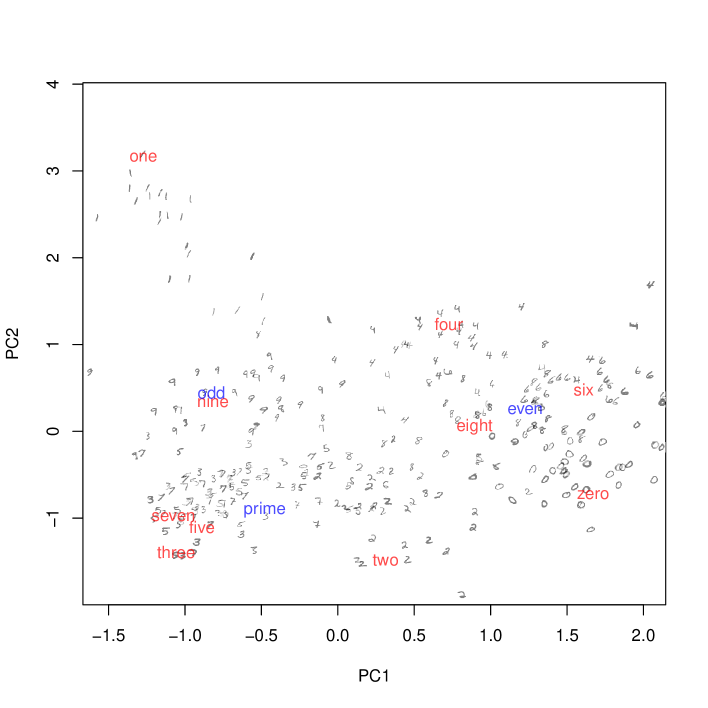
Figure 1: Scatter plot of the first two components of CDMCA for the MNIST handwritten digits. Shown are 300 digit images randomly sampled from the 60000 training images ($d=1$). Digit labels ($d=2$) and attribute labels ($d=3$) are also shown in the same “common space” of $K=2$.

(a) classification errors ($K=9$)

(b) matching errors ($K=9$)

Figure 2: CDMCA results for $\gamma_{M}=10^{-4},10^{-3},10^{-2},10^{-1},10^{0},10^{1}$. (a) Classification error of predicting digit labels ($d=2$) from the 10000 test images, and that for predicting attribute labels ($d=3$). (b) The true matching error of 10000 test images, and the fitting error and the cross-validation error computed from the 60000 training images.

(a) $\bm{\bar{W}}_{A}$

(b) $\bm{W}$ of Experiment 1

(c) $\bm{W}$ of Experiment 9

Figure 3: Regular matching weights. (a) A true matching weight of a regular structure. (b) Link sampling from $\bm{\bar{W}}_{A}$. (c) Node sampling from $\bm{\bar{W}}_{A}$.

(a) $\bm{\bar{W}}_{B}$

(b) $\bm{W}$ of Experiment 5

(c) $\bm{W}$ of Experiment 11

Figure 4: Power-law matching weights. (a) A true matching weight of a power-law structure. (b) Link sampling from $\bm{\bar{W}}_{B}$. (c) Node sampling from $\bm{\bar{W}}_{B}$.

(a) fitting error

(b) cv error (link)

(c) cv error (node)

Figure 7: Bias of the matching errors of the components rescaled by the weighted variance (2).

(a) fitting error

(b) cv error (link)

(c) cv error (node)

Figure 8: Bias of the matching errors of the components rescaled by the unweighted variance (9).

References

• Belkin and Niyogi (2003) {barticle}[author] \bauthor\bsnmBelkin, \bfnmMikhail\binitsM. and \bauthor\bsnmNiyogi, \bfnmPartha\binitsP. (\byear2003). \btitleLaplacian eigenmaps for dimensionality reduction and data representation. \bjournalNeural computation \bvolume15 \bpages1373–1396. \endbibitem
• Chung (1997) {bbook}[author] \bauthor\bsnmChung, \bfnmFan RK\binitsF. R. (\byear1997). \btitleSpectral graph theory \bvolume92. \bpublisherAmerican Mathematical Soc. \endbibitem
• Correa et al. (2010) {barticle}[author] \bauthor\bsnmCorrea, \bfnmNicolle M\binitsN. M., \bauthor\bsnmEichele, \bfnmTom\binitsT., \bauthor\bsnmAdalı, \bfnmTülay\binitsT., \bauthor\bsnmLi, \bfnmYi-Ou\binitsY.-O. and \bauthor\bsnmCalhoun, \bfnmVince D\binitsV. D. (\byear2010). \btitleMulti-set canonical correlation analysis for the fusion of concurrent single trial ERP and functional MRI. \bjournalNeuroimage \bvolume50 \bpages1438–1445. \endbibitem
• Daumé III (2009) {binproceedings}[author] \bauthor\bsnmDaumé III, \bfnmHal\binitsH. (\byear2009). \btitleFrustratingly easy domain adaptation. In \bbooktitleProceedings of the 45th Annual Meeting of the Association of Computational Linguistics \bpages256–263. \endbibitem
• Golub, Heath and Wahba (1979) {barticle}[author] \bauthor\bsnmGolub, \bfnmGene H\binitsG. H., \bauthor\bsnmHeath, \bfnmMichael\binitsM. and \bauthor\bsnmWahba, \bfnmGrace\binitsG. (\byear1979). \btitleGeneralized cross-validation as a method for choosing a good ridge parameter. \bjournalTechnometrics \bvolume21 \bpages215–223. \endbibitem
• Gong et al. (2014) {barticle}[author] \bauthor\bsnmGong, \bfnmYunchao\binitsY., \bauthor\bsnmKe, \bfnmQifa\binitsQ., \bauthor\bsnmIsard, \bfnmMichael\binitsM. and \bauthor\bsnmLazebnik, \bfnmSvetlana\binitsS. (\byear2014). \btitleA multi-view embedding space for modeling internet images, tags, and their semantics. \bjournalInternational Journal of Computer Vision \bvolume106 \bpages210–233. \endbibitem
• Hastie, Tibshirani and Friedman (2009) {bbook}[author] \bauthor\bsnmHastie, \bfnmTrevor\binitsT., \bauthor\bsnmTibshirani, \bfnmRobert\binitsR. and \bauthor\bsnmFriedman, \bfnmJerome\binitsJ. (\byear2009). \btitleThe Elements of Statistical Learning. Data Mining, Inference, and Prediction, Second Edition. \bpublisherSpringer. \endbibitem
• Hotelling (1936) {barticle}[author] \bauthor\bsnmHotelling, \bfnmHarold\binitsH. (\byear1936). \btitleRelations between two sets of variates. \bjournalBiometrika \bvolume28 \bpages321–377. \endbibitem
• Huang et al. (2013) {bincollection}[author] \bauthor\bsnmHuang, \bfnmZhiwu\binitsZ., \bauthor\bsnmShan, \bfnmShiguang\binitsS., \bauthor\bsnmZhang, \bfnmHaihong\binitsH., \bauthor\bsnmLao, \bfnmShihong\binitsS. and \bauthor\bsnmChen, \bfnmXilin\binitsX. (\byear2013). \btitleCross-view graph embedding. In \bbooktitleComputer Vision – ACCV 2012, Revised Selected Papers, Part II \bpages770–781. \bpublisherSpringer. \endbibitem
• Kan et al. (2012) {bincollection}[author] \bauthor\bsnmKan, \bfnmMeina\binitsM., \bauthor\bsnmShan, \bfnmShiguang\binitsS., \bauthor\bsnmZhang, \bfnmHaihong\binitsH., \bauthor\bsnmLao, \bfnmShihong\binitsS. and \bauthor\bsnmChen, \bfnmXilin\binitsX. (\byear2012). \btitleMulti-view discriminant analysis. In \bbooktitleComputer Vision – ECCV 2012, Proceedings, Part I \bpages808–821. \bpublisherSpringer. \endbibitem
• Kettenring (1971) {barticle}[author] \bauthor\bsnmKettenring, \bfnmJon R\binitsJ. R. (\byear1971). \btitleCanonical analysis of several sets of variables. \bjournalBiometrika \bvolume58 \bpages433–451. \endbibitem
• Kohonen (1972) {barticle}[author] \bauthor\bsnmKohonen, \bfnmTeuvo\binitsT. (\byear1972). \btitleCorrelation matrix memories. \bjournalComputers, IEEE Transactions on \bvolume100 \bpages353–359. \endbibitem
• LeCun et al. (1998) {barticle}[author] \bauthor\bsnmLeCun, \bfnmYann\binitsY., \bauthor\bsnmBottou, \bfnmLéon\binitsL., \bauthor\bsnmBengio, \bfnmYoshua\binitsY. and \bauthor\bsnmHaffner, \bfnmPatrick\binitsP. (\byear1998). \btitleGradient-based learning applied to document recognition. \bjournalProceedings of the IEEE \bvolume86 \bpages2278–2324. \endbibitem
• Mikolov et al. (2013) {binproceedings}[author] \bauthor\bsnmMikolov, \bfnmTomas\binitsT., \bauthor\bsnmSutskever, \bfnmIlya\binitsI., \bauthor\bsnmChen, \bfnmKai\binitsK., \bauthor\bsnmCorrado, \bfnmGreg S\binitsG. S. and \bauthor\bsnmDean, \bfnmJeff\binitsJ. (\byear2013). \btitleDistributed representations of words and phrases and their compositionality. In \bbooktitleAdvances in Neural Information Processing Systems 26 \bpages3111–3119. \endbibitem
• Nakano (1972) {barticle}[author] \bauthor\bsnmNakano, \bfnmKaoru\binitsK. (\byear1972). \btitleAssociatron – A model of associative memory. \bjournalSystems, Man and Cybernetics, IEEE Transactions on \bvolume3 \bpages380–388. \endbibitem
• Nori, Bollegala and Kashima (2012) {binproceedings}[author] \bauthor\bsnmNori, \bfnmNozomi\binitsN., \bauthor\bsnmBollegala, \bfnmDanushka\binitsD. and \bauthor\bsnmKashima, \bfnmHisashi\binitsH. (\byear2012). \btitleMultinomial Relation Prediction in Social Data: A Dimension Reduction Approach. In \bbooktitleProceedings of the Twenty-Sixth AAAI Conference on Artificial Intelligence (AAAI-12) \bpages115–121. \endbibitem
• Olshausen and Field (2004) {barticle}[author] \bauthor\bsnmOlshausen, \bfnmBruno A\binitsB. A. and \bauthor\bsnmField, \bfnmDavid J\binitsD. J. (\byear2004). \btitleSparse coding of sensory inputs. \bjournalCurrent opinion in neurobiology \bvolume14 \bpages481–487. \endbibitem
• Shi et al. (2013) {barticle}[author] \bauthor\bsnmShi, \bfnmXiaoxiao\binitsX., \bauthor\bsnmLiu, \bfnmQi\binitsQ., \bauthor\bsnmFan, \bfnmWei\binitsW. and \bauthor\bsnmYu, \bfnmPhilip S\binitsP. S. (\byear2013). \btitleTransfer across completely different feature spaces via spectral embedding. \bjournalKnowledge and Data Engineering, IEEE Transactions on \bvolume25 \bpages906–918. \endbibitem
• Stone (1977) {barticle}[author] \bauthor\bsnmStone, \bfnmMervyn\binitsM. (\byear1977). \btitleAn asymptotic equivalence of choice of model by cross-validation and Akaike’s criterion. \bjournalJournal of the Royal Statistical Society. Series B (Methodological) \bpages44–47. \endbibitem
• Takane, Hwang and Abdi (2008) {barticle}[author] \bauthor\bsnmTakane, \bfnmYoshio\binitsY., \bauthor\bsnmHwang, \bfnmHeungsun\binitsH. and \bauthor\bsnmAbdi, \bfnmHervé\binitsH. (\byear2008). \btitleRegularized multiple-set canonical correlation analysis. \bjournalPsychometrika \bvolume73 \bpages753–775. \endbibitem
• Tenenhaus and Tenenhaus (2011) {barticle}[author] \bauthor\bsnmTenenhaus, \bfnmArthur\binitsA. and \bauthor\bsnmTenenhaus, \bfnmMichel\binitsM. (\byear2011). \btitleRegularized generalized canonical correlation analysis. \bjournalPsychometrika \bvolume76 \bpages257–284. \endbibitem
• Van Der Aa, Ter Morsche and Mattheij (2007) {barticle}[author] \bauthor\bsnmVan Der Aa, \bfnmNP\binitsN., \bauthor\bsnmTer Morsche, \bfnmHG\binitsH. and \bauthor\bsnmMattheij, \bfnmRRM\binitsR. (\byear2007). \btitleComputation of eigenvalue and eigenvector derivatives for a general complex-valued eigensystem. \bjournalElectronic Journal of Linear Algebra \bvolume16 \bpages300–314. \endbibitem
• Von Luxburg (2007) {barticle}[author] \bauthor\bsnmVon Luxburg, \bfnmUlrike\binitsU. (\byear2007). \btitleA tutorial on spectral clustering. \bjournalStatistics and computing \bvolume17 \bpages395–416. \endbibitem
• Wang et al. (2013) {binproceedings}[author] \bauthor\bsnmWang, \bfnmKaiye\binitsK., \bauthor\bsnmHe, \bfnmRan\binitsR., \bauthor\bsnmWang, \bfnmWei\binitsW., \bauthor\bsnmWang, \bfnmLiang\binitsL. and \bauthor\bsnmTan, \bfnmTieniu\binitsT. (\byear2013). \btitleLearning coupled feature spaces for cross-modal matching. In \bbooktitleComputer Vision (ICCV), 2013 IEEE International Conference on \bpages2088–2095. \bpublisherIEEE. \endbibitem
• Yan et al. (2007) {barticle}[author] \bauthor\bsnmYan, \bfnmShuicheng\binitsS., \bauthor\bsnmXu, \bfnmDong\binitsD., \bauthor\bsnmZhang, \bfnmBenyu\binitsB., \bauthor\bsnmZhang, \bfnmHong-Jiang\binitsH.-J., \bauthor\bsnmYang, \bfnmQiang\binitsQ. and \bauthor\bsnmLin, \bfnmStephen\binitsS. (\byear2007). \btitleGraph embedding and extensions: a general framework for dimensionality reduction. \bjournalPattern Analysis and Machine Intelligence, IEEE Transactions on \bvolume29 \bpages40–51. \endbibitem
• Yuan and Sun (2014) {barticle}[author] \bauthor\bsnmYuan, \bfnmYun-Hao\binitsY.-H. and \bauthor\bsnmSun, \bfnmQuan-Sen\binitsQ.-S. (\byear2014). \btitleGraph regularized multiset canonical correlations with applications to joint feature extraction. \bjournalPattern Recognition \bvolume47 \bpages3907–3919. \endbibitem
• Yuan et al. (2011) {barticle}[author] \bauthor\bsnmYuan, \bfnmYun-Hao\binitsY.-H., \bauthor\bsnmSun, \bfnmQuan-Sen\binitsQ.-S., \bauthor\bsnmZhou, \bfnmQiang\binitsQ. and \bauthor\bsnmXia, \bfnmDe-Shen\binitsD.-S. (\byear2011). \btitleA novel multiset integrated canonical correlation analysis framework and its application in feature fusion. \bjournalPattern Recognition \bvolume44 \bpages1031–1040. \endbibitem