ETEAPOT: symplectic orbit/spin tracking code for all-electric storage rings

Abstract

Proposed methods for measuring the electric dipole moment (EDM) of the proton use an intense, polarized proton beam stored in an all-electric storage ring “trap”. At the “magic” kinetic energy of 232.792 MeV, proton spins are “frozen”, for example always parallel to the instantaneous particle momentum. Energy deviation from the magic value causes in-plane precession of the spin relative to the momentum. Any non-zero EDM value will cause out-of-plane precession—measuring this precession is the basis for the EDM determination. A proposed implementation of this measurement shows that a proton EDM value of $10^{-29}\,$e-cm or greater will produce a statistically-significant, measurable precession after multiply-repeated runs, assuming small beam depolarization during 1000 second runspEDM-PRL , with high enough precision to test models of the early universe developed to account for the present day particle/anti-particle population imbalance.

This paper describes an accelerator simulation code, ETEAPOT, a new component of the Unified Accelerator Libraries (UAL), to be used for long term tracking of particle orbits and spins in electric bend accelerators, in order to simulate EDM storage ring experiments. Though qualitatively much like magnetic rings, the non-constant particle velocity in electric rings give them significantly different properties, especially in weak focusing rings. Like the earlier code TEAPOT (for magnetic ring simulation) this code performs exact tracking in an idealized (approximate) lattice rather than the more conventional approach, which is approximate tracking in a more nearly exact lattice. The BMT equation describing the evolution of spin vectors through idealized bend elements is also solved exactly—original to this paper. Furthermore the idealization permits the code to be exactly symplectic (with no artificial “symplectification”). Any residual spurious damping or anti-damping is sufficiently small to permit reliable tracking for the long times, such as the 1000 seconds assumed in estimating the achievable EDM precision.

This paper documents in detail the theoretical formulation implemented in ETEAPOT. The accompanying paperAGSAnalogue “EDM planning using ETEAPOT with a resurrected AGS Electron Analogue ring” describes the practical application of the ETEAPOT code in the UAL environment to “resurrect”, or reverse-engineer, the “AGS-Analogue” all-electric ring built at Brookhaven National Laboratory in 1954. Of the (very few) all-electric rings ever commissioned, the AGS-Analogue ring is the only relativistic one and is the closest to what is needed for measuring proton (or, even more so, electron) EDM’s. That paper also describes preliminary lattice studies for the planned proton EDM storage rings as well as testing the code against analytic calculations.

I Introduction

Orbit and spin simulation code needed for electric storage rings.

The U.S. particle physics community has recently updated its vision of the future and strategy for the next decade in a Particle Physics Project Prioritization Panel (P5) Report. One of the physics goals endorsed by P5 is measuring the EDM of fundamental particles (in particular proton, deuteron, neutron and electron).

Since Standard Model EDM predictions are much smaller than current experimental sensitivities, detection of any particle’s non-zero EDM would signal discovery of New Physics. If of sufficient strength, such a source could provide an explanation for the observed matter/antimatter asymmetry of our universe. A proton EDM collaborationpEDM-PRL has proposed a storage ring proton EDM measurement at the unprecedented level of $10^{-29}e\cdot\,$cm, an advance by nearly 5 orders of magnitude beyond the current indirect bound obtained using Hg atoms.

This paper is limited to the theoretical orbit and spin dynamical formulation within ETEAPOT, which is a newly developed code within the Universal Accelerator Libraries (UAL) simulation environment. The accompanying paper “Using ETEAPOT to resurrect the AGS-Analogue ring for EDM planning” describes the practical application of the ETEAPOT code with emphasis on details of simulation requirements for the EDM measurement.

Complications imposed by electric bending.

The fundamental complication of an electric ring, as contrasted to a magnetic ring, is the non-constancy of particle speed. A fast/slow separation into betatron and synchrotron amplitudes has become fundamental to the conventional (Courant-Snyder) magnetic ring formalism. But, in an electric lattice the mechanical energy (as quantified by the relativistic factor $\gamma=1/\sqrt{1-\beta^{2}}$) varies on the same time scale as the transverse $x$ and $y$ amplitudes. On the other hand, changing only in RF cavities, the total energy $\mathcal{E}=\gamma mc^{2}+eV(r)$, which includes also the potential energy $eV(r)$, changes on a slow time scale, which makes a similar fast/slow separation valid.

In the magnetic formalism, since it is only in RF cavities that the mechanical energy varies, the $\gamma$ factor is invariant in the rest of the ring. Furthermore one is accustomed to treating energy as constant for times short compared to the synchrotron period. To the extent the betatron parameters are independent of particle energy, the betatron and synchrotron motions can then be superimposed.

To most closely mimic this treatment in an electric ring, and to continue to regard $\gamma$ as the fundamental “energy-like” parameter, requires us to evaluate $\gamma$ only in regions of zero electric potential, which is to say, not in RF cavities, and not in electric bending elements—in other words, only in field free drift regions. This leads to a curious, but entirely satisfactory, representation in which the particles spend most of their time inside bend elements where $\gamma$ is varying, and little time in short drift regions where $\gamma$ is constant. The reason this is fully satisfactory is that the drift regions are closely spaced, and more or less uniformly spaced around the ring. Knowing the lattice functions exactly at those points is operationally equivalent to knowing them everywhere. With this interpretation, one can again rely on the approximate representation of the motion as a superposition of fast betatron and slow synchrotron motions.

II Particle tracking paradigms

The conventional formulation of accelerator physics is based on a paraxial approximation in which all orbit angles are small relative to a central design orbit. Not only is this approximation quite good for small rings, it becomes progressively better as ring radii increase. The most important formulas obtained in this approach are based on linearization of the paraxial orbit equations. For sufficiently small amplitudes orbit evolution can be represented by “transfer matrices” multiplying initial displacements, represented in 6D phase space by six component displacement vectors. By introducing nonlinear “transfer maps” this approach can be extended to larger amplitudes by representing each output variable as a (truncated) power series of terms each of which is a product of initial components, or their squares, cubes, etc. This approach can be referred to as approximate tracking in an “exact” lattice where “exact” means, for example, that magnetic field profiles, fringe fields etc., once represented faithfully by accurate power series, can be subsumed into the previously described truncated power series orbit representations.

The TEAPOT tracking paradigmTEAPOT is very different. It is a refinement of the “kick code” paradigm, under development when TEAPOT was first introduced, about thirty years ago. Though still based on the paraxial approximation, elements are sliced into sufficiently short segments that they can be represented by delta function “kicks”, or kinks, where orbit slopes change discontinuously, but displacements are continuous. The main virtue of this approach is that it is symplectic; i.e. particle beams respect Liouville’s theorem.

TEAPOT took the more extreme approach of jettisoning the paraxial approximation altogether, and insisting that orbits be constructed only from exactly determined, analytic orbits, interupted where appropriate, by kicks. This can be referred to as exact tracking in an approximate lattice. This approach is restricted by the fact that exact orbits are known only in very special cases; for example in uniform magnetic fields. However, by introducing thin kick elements it is possible to represent actual elements and actual rings to good accuracy. These added kicks may be artificial, meaning they model field deviations from the idealized field, or they may represent the total fields of elements physically present in the lattice. All this is explained in detail in the original Schachinger and Talman paperTEAPOT , which remains valid, and in use, to this day. To restrict the length of the present paper, only features newly introduced in ETEAPOT, and not covered in the original paper, are described.

One new feature is the requirement to use electric rather than magnetic bending elements, which brings in the complication already mentioned, that, unlike in magnets, particle speeds are not constant in electric elements. The other new feature is the need to also track the particle spins. To respect the TEAPOT paradigm this further restricts the list of allowable lattice elements to elements for which the BMT equation, an abbreviation for Michel, Bargmann, and TelegdiBMT , is exactly solvable. Fortunately it is possible, even straightforward, to meet both of these new restrictions.

The ETEAPOT approach has been developed to address new requirements of the proton EDM project. First is the transition from mgnetic to electric bending. Magnetic tracking codes like TEAPOT and MAD implicitly take advantage of the constant speed of particles in magnetic fields. This seriously complicates the porting of simulation algorithms to electric rings in which the particle speed depends on the local electric potential energy. Thick bending elements are again to be replaced by integrable force fields. As it happens, Inverse square law is the unique force field for which the 3D relativistic equations of motion can be solved exactly. The second major ETEAPOT extension has been the introduction and tracking of particle spin vectors (which provides the EDM signature of the EDM experiment). The differential equation governing spin motion is the BMT equation. In general 3D motion the BMT equations are computationally challenging. But in our idealized elements the BMT equations can be solved exactly, as required by the fundamental TEAPOT/ETEAPOT design principle.

By symmetry, every orbit in a radial force field lies in a plane, referred to here as “the bend plane”. This plane is always close to but, in general, not quite identical to the horizontal symmetry of the ring. In spherical $(r,\theta)$ coordinates the differential equation governing $r(\theta)$ for a relativistic particle orbit in an inverse square law force field can be solved exactlyMunoz . These are like classical planetary orbits or the orbits in a hydrogen atom treated classically. Even relativistically, every orbit is a precessing ellipse-like (rosette) figure, familiar to Newton in classical mechanics, and for relativistic motion to Einstein, in his general relativistic calculation of the advance of the perihelion of Mercury.

Using $(r,\theta)$ polar coordinates, it will be shown shortly that orbit evolution in an inverse square law bend plane is described exactly by

$$r(\theta)=\frac{\lambda}{1+\epsilon\cos\kappa(\theta-\theta_{0})},\quad\hbox{and}\quad x=r-r_{0}$$ (1)

where $r$ is the radial distance from the bend center to the particle position. Then $x$ is the (paraxial) radial displacement from the design central orbit, which is a circle of radius $r_{0}$. This formula is as simple as it is only because the motion is two dimensional. The potential energy depends only on $r(\theta)$, permitting the speed, and hence the momentum components to be expressed analytically as functions of $\theta$. In correlating this equation with conventional paraxial treatment, one notes that the independent variable $\theta$ here differs from the independent longitudinal variable $s$, which is the path length along the design orbit; but $s$ and $\theta$ advance proportionally in bend elements, with the constant of proportionality being the design radius $r_{0}$.

Each particle being tracked has its own private orbit plane parameters in the orbit equation—though they are all very nearly the same for realistic beams. The parameters in Eq. (1) are interpretable (approximately) as follows: $\lambda$ is “average” radius, $\epsilon$ is “eccentricity”, $\theta_{0}$ is the angular deviation from perihelion, and $\kappa$ (interpretable as the “tune” in accelerator jargon) establishes the betatron phase advance per unit angular advance.

For particle tracking this formulation is simpler than the 3D description of orbits in a uniform magnetic field. One price to be paid for this simplicity is the need to transform each particle into, and later, out of, its private 2D orbit plane (with its own basis vectors) as it enters, and later, leaves a bending element. These transformations, not shown here, are elementary near-identity rigid rotations (including spin).

A more serious price for this exact, “global” coordinate, approach is purely numerical. Though Eq. (1) is analytically exact it is numerically treacherous—the paraxial quantity $x$ is a millimeter scale length compared to $r$ which is very nearly equal to the $r_{0}$ which is a large length, such as 40 m. The special numerical treatment needed to handle this issue is discussed below.

III Relativistic kinematics in electric potential $V(r)$.

In the horizontal $y$=0 bend plane, a radial electric field with index $m$ power law dependence on radius $r$ is

$${\bf E}(r,0)=-E_{0}\,\frac{r_{0}^{1+m}}{r^{1+m}}\,{\bf\hat{r}},$$ (2)

and the electric potential $V(r)$, adjusted to vanish at $r=r_{0}$, is

$$V(r)=-\frac{E_{0}r_{0}}{m}\,\bigg{(}\frac{r_{0}^{m}}{r^{m}}-1\bigg{)}.$$ (3)

The “cleanest” case, shown in Figure 1, has $m$=1 and is known as the Kepler or the Coulomb electric field of a point source. One way our case is more general than Kepler’s is that our treatment has to be exactly relativistic. This $m$=1 case can be referred to as “spherical” since the equipotentials are spheres centered on a point charge at the center, and $r$ is the radius in $(r,\theta,\phi)$ spherical coordinates. For $m$=1 the Kepler problem can be solved in closed form with the same generality as in the relativistic as in the nonrelativistic case. However the orbits are no longer exactly elliptical, nor restricted to a single plane.

The $m$=0 field is referred to as “cylindrical” and $r$ is the radius in $(r,\phi,y)$ cylindrical coordinates. This field is the experimentally easiest to produce, using cylindical electrodes having the same central axis. It has been tacitly assumed that the EDM storage ring bends will be constructed this way, even if the optimal electrode shape would be somewhat different. As already explained, (weak) thin quadrupoles can be used to tailor the fields to overcome this impediment. Curved-planar electrodes produce the electric field shown in Figure 2

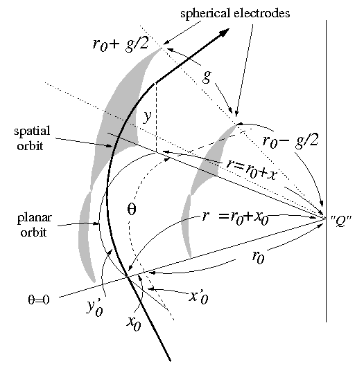
Figure 1: The bold curve shows a particle orbit passing through a spherical, $m=1$, electrostatic bending element. The shaded surfaces are electrodes and the figure is grossly distorted. The “$Q$” shown at the origin is the “effective point charge” that would give the same idealized electric field as the electrodes.

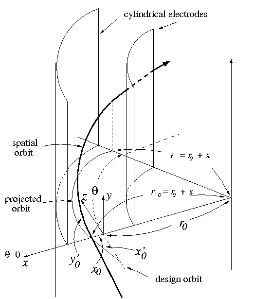
Figure 2: The bold curve shows a particle orbit passing through a curved-planar cylindrical, $m=0$, electrostatic bending element. The electrode spacing is $g$ and the design orbit is centered between the electrodes in the $y$=0 plane.

Solution of the equation of motion.

Throughout much of this section formulas of Muñoz and PavicMunoz will be transcribed essentially unchanged, except for bringing symbols into consistency with conventional accelerator notation. The Muñoz/Pavic formulation, though equivalent to various other formalisms describing relativistic Coulomb orbits, is especially appropriate for our relativistic accelerator application. Muñoz and Pavic show that the “generalized”-Hamilton vector

$$\widetilde{\bf h}=\widetilde{h_{r}}\,{\bf\hat{r}}+\widetilde{h_{\theta}}\,{\hat{\bm{\theta}}}$$ (4)

is especially useful for describing 2D relativistic Kepler orbits. Our 3D accelerator application can be formulated in such a way as to use only such 2D orbits. Except for scale factors, and a $\gamma$-dependent offset, the pair $(\tilde{h}_{r},\tilde{h}_{\theta})$ will reduce to the conventional phase space coordinates $(x,x^{\prime})$.

In accelerator context the evolution of $\widetilde{\bf h}$ for any particular particle will be interpretable as the phase space evolution of that particle. We will refer to $\widetilde{\bf h}$ as the “MP-vector” since, as far as we know, Muñoz and Pavic intoduced it. In the non-relativistic regime $\widetilde{\bf h}$ is related to the (nonrelativistically conserved) Laplace-Runge-Lenz vector. As generalized by Muñoz and Pavic, though not quite conserved in the relativistic regime, $\widetilde{\bf h}$ satisfies a very simple equation of motion, whose exact solutions are sinusoids, even at arbitrarily large “betatron” amplitudes.

In geometric mechanics jargonRT-GM , the lattice is therefore “integrable”. The $\widetilde{\bf h}$ formalism then makes it possible to define an implicit transfer matrix (where “implicit” implies the matrix elements depend on each particle’s own conserved orbit parameters, a.k.a. “orbit elements”). This has the virtue of hiding the strong coupling between kinetic energy and horizontal position in an electric ring.

Though $\widetilde{\bf h}$ is not conserved in general, Muñoz and Pavic show (and it will soon become obvious) that $\widetilde{\bf h}$ is conserved if and only if the orbit is circular. For the proton EDM lattice the design orbit is circular within bends. Also, for weak-focusing lattices, neglecting the effects of lattice quadrupoles situated between the bends, off-momentum closed orbits are also almost circlular.

But $\widetilde{\bf h}$ also has the numerical disadvantage mentioned earlier—transverse displacements (the normally significant aspect of accelerator dynamics) need, at least superficially, to be described by expressions having large cancellations. This makes it essential to use series approximations very carefully, even when the linearized paraxial approximation is fully valid. It is important to organize the evolution formulas in such a way as to exploit cancellations analytically, for example arranging for leading terms to cancel analytically, rather than relying on their numerical cancellation. This can usually be accomplished (without sacrificing exact expressions) by simplifying the sum of the approximately cancelling terms and keeping track and restoring any discrepancy. This recovers numerical precision for small amplitudes comparable to that achieved in conventional Courant-Snyder formulation.

Another inconvenient aspect of the Muñoz/Pavic formalism is the fact that the design, central orbit is degenerate in the sense that it is, in fact, the arc of a perfect circle. This is precisely the condition in which the perihelion (or aphelion) angular orbit element is undefined because the radius vector length is independent of angular position. This ambiguity is most important in the time of flight calculations needed for accurate modeling of synchrotron (longitudinal) oscillations—a calculation that strains the numerical accuracy because all path lengths are so nearly equal.

These same considerations complicate the derivation of explicit (meaning the elements are independent of particle coordinates) transfer matrices and their generalization to truncated power series transfer maps. This also is only a inconvenience that can be worked around.

With qualitative discussion complete, the analytic formulation can begin. The Lorentz force equation in the $m$=1 spherical case is

$$\frac{d{\bf p}}{dt}=-k\,\frac{{\bf\hat{r}}}{r^{2}},$$ (5)

where $k$ is the customary MKS notation for $1/(4\pi\epsilon_{0})$ except for implicitly including also the (point) charge factor. On the central orbit the centripetal force equation is

$$\frac{(p_{0}c/e)\beta_{0}}{r_{0}}=\frac{k/e}{r_{0}^{2}}\overset{\rm also}{\ =\ }E_{0}.$$ (6)

where $k$, like $E_{0}$, the on-axis electric field, is defined to be positive. In UAL, as in the MAD simulation code, energies like $p_{0}c$ are always expressed numerically in GeV units, such that their numerical value in the computer is $10^{-9}p_{0}c/e$, giving them GV units—an MKS unit. From Eq. (6), $k/e$=$(p_{0}c/e)\beta_{0}r_{0}$ and $k$ is always expressed in the computer as $10^{-9}k/e$, which gives it GV-m units—also an MKS unit. The on-axis electric field $E_{0}$ is measured in GV/m units. In these units $k=E_{0}r_{0}^{2}$, numerically, with $r_{0}$ measured in meters.

A particle’s angular momentum is

$${\bf L}={\bf r}\times{\bf p}.$$ (7)

In terms of the design momentum $p_{0}$ and the design radius $r_{0}$, $L_{0}=r_{0}p_{0}$, and

$$\frac{k}{L_{0}c}=\beta_{0}\quad(=0.598379\ {\rm for\ pEDM}).$$ (8)

Like $k$, internally (i.e. in the computer), $L_{0}c$ is expressed numerically as $10^{-9}L_{0}c/e$. For internal numerical values to be most easily substituted into an analytic external documentation formula, factors should be grouped as $pc/e$, $Lc/e$, $k/e$, etc. or, as here, $k/(Lc)$, and factors of $10^{9}$ (for eV to GeV conversion) put in “by hand”. Eq. (8) is also useful in the form

$$k=\gamma_{0}m_{p}c^{2}r_{0}\beta^{2}_{0}.$$ (9)

In SXF lattice description files (discussed further in the accompanying paperAGSAnalogue ) the RF parameter $V$ actually stands for $10^{-9}$ times the maximum energy change in eV of charge $e$ passing through the RF cavity.

One shows easily that both the total energy

$$\mathcal{E}=\Big{(}\gamma^{I}m_{p}c^{2}-\frac{k}{r}\Big{)}+\frac{k}{r_{0}}\equiv\mathcal{E}_{M}+\frac{k}{r_{0}},$$ (10)

(where the “I” superscript on $\gamma^{I}$ re-emphasizes that this relativistic factor has to be evaluated “inside” the bend element, where it depends on the local electric potential) and the angular momentum

$$L=\gamma^{I}m_{p}r^{2}\dot{\theta},$$ (11)

are constants of the motion. It has been necessary to distinguish between the Muñoz potential energy $eV_{M}$ and our potential energy $eV$, because our potential vanishes on the design orbit, while theirs vanishes at infinity. For the design orbit, using Eqs. (9) and (10), one obtains

$$\mathcal{E}_{M,0}=\frac{m_{p}c^{2}}{\gamma_{0}}.$$ (12)

(The curious presence of $\gamma_{0}$ in the denominator follows from the definition of potential energy.) Using the obvious unit vector relations (valid for motion with angle $\theta$ increasing)

$${\hat{\bm{\theta}}}^{\prime}=-{\bf\hat{r}},\quad\hbox{and}\quad{\bf\hat{r}}^{\prime}={\hat{\bm{\theta}}},$$ (13)

where primes stand for $d/d\theta$, the Lorentz equation can be re-expressed as

$$\frac{d{\bf p}}{dt}=\frac{k}{r^{2}}\,\frac{d{\hat{\bm{\theta}}}}{d\theta}.$$ (14)

Defining covariant velocity ${\bf u}=\gamma^{I}{\bf v}$, and using Eq. (11) to express $d\theta/dt$ in terms of $L$, the ${\bf u}$ equation of motion is

$$\frac{d{\bf u}}{d\theta}=\frac{k\gamma^{I}}{L}\,\frac{d{\hat{\bm{\theta}}}}{d\theta}.$$ (15)

Muñoz and Pavic then introduce the generalized Hamilton vector

$$\widetilde{\bf h}={\bf u}-\frac{k\gamma^{I}}{L}\,{\hat{\bm{\theta}}},\quad\hbox{or}\quad(\widetilde{h}_{\theta},\widetilde{h}_{r})=\Big{(}u_{\theta}-\frac{k\gamma^{I}}{L},u_{r}\Big{)},$$ (16)

which we refer to as the MP-vector. It is specially tailored so that the differential equation for $\widetilde{\bf h}$ reduces to

$$\frac{d\widetilde{\bf h}}{d\theta}=-\frac{k}{L}\,\frac{d\gamma^{I}}{d\theta}\,{\hat{\bm{\theta}}}.$$ (17)

(The previously mentioned constancy of $\widetilde{\bf h}$ on circular orbits is evident from this equation, since $\gamma^{I}$ is constant on, and only on, circular orbits.) Using

$$u_{\theta}=\frac{L}{m_{p}r},\quad\hbox{}\quad\widetilde{h}_{\theta}=\frac{L}{m_{p}r}-\frac{k\gamma^{I}}{L}\overset{\rm also}{\ =\ }\frac{\kappa^{2}L}{m_{p}r}-\frac{k}{L}\,\frac{\mathcal{E}_{M}}{m_{p}c^{2}},$$ (18)

where the new parameter $\kappa$ (soon to be identified as horizontal betatron “tune”) is defined by

$$\kappa^{2}=1-\bigg{(}\frac{k}{Lc}\bigg{)}^{2}.$$ (19)

On the design orbit

$$\kappa_{0}=\sqrt{1-\beta_{0}^{2}}=\frac{1}{\gamma_{0}}\quad(=\ 0.801213\ {\rm for\ pEDM}).$$ (20)

(Of course $\kappa_{0}$ will not be controlled to this accuracy in practice and, in any case, quadrupoles and drifts in the lattice will alter the ring tunes.) Solving Eq. (18) for $r$, the orbit equation in bend elements can be expressed in terms of $\widetilde{h}_{\theta}$;

$$r=\frac{\lambda}{1+\bar{\epsilon}\widetilde{h}_{\theta}},$$ (21)

where

$$\lambda=\frac{L^{2}c^{2}\kappa^{2}}{k\mathcal{E}_{M}}\quad\hbox{and}\quad\bar{\epsilon}=\frac{m_{p}c^{2}}{\mathcal{E}_{M}}\,\frac{L}{k}.$$ (22)

The parameter $\lambda$ is especially important in the storage ring context, because the second term in the denominator of Eq. (21) is both small compared to the first, and oscillatory. As a result $\lambda$ can be thought of loosely as an average radial position. (As earlier, the “constants of motion” $L$, $\kappa$, $\bar{\epsilon}$, and $\lambda$ are to be referred to as “orbit elements”. Though constant along any single particle orbit, they are different (though only very slightly) for each individual particle.)

In component form Eq. (17) is

$$\widetilde{h}_{r}^{\prime}-\widetilde{h}_{\theta}=0,\quad\widetilde{h}_{\theta}^{\prime}+\widetilde{h}_{r}=-\frac{k}{L}\,{\gamma^{I}}^{\prime}.$$ (23)

The relativistic factor $\gamma^{I}$ (equal to $(\mathcal{E}_{M}+k/r)/(m_{p}c^{2})$) can be expressed in terms of $\widetilde{h}_{\theta}$. First, eliminate $r$ in favor of $u_{0}$ using the first of Eqs. (18), then eliminate $u_{0}$ if favor of $\widetilde{h}_{\theta}$, and, finally, solve for $\gamma^{I}$;

$$\gamma^{I}=\frac{\mathcal{E}_{M}}{\kappa^{2}m_{p}c^{2}}+\frac{k}{\kappa^{2}Lc^{2}}\,\widetilde{h}_{\theta}.$$ (24)

Needed for simplifying Eqs. (23), differentiating this equation yields

$${\gamma^{I}}^{\prime}=\frac{k}{\kappa^{2}Lc^{2}}\,\widetilde{h}^{\prime}_{\theta}.$$ (25)

(Heuristically, this expresses the dependence of mechanical energy accompanying the change in potential energy associated with change in particle position.) After several lines of algebra, Eqs. (23) then reduce to

$$\boxed{\begin{aligned} \widetilde{h}_{r}^{\prime}&=\widetilde{h}_{\theta},\\ \widetilde{h}_{\theta}^{\prime}&=-\kappa^{2}\,\widetilde{h}_{r}.\end{aligned}}$$ (26)

These are the equations that justify having introduced the generalized Hamilton vector. Their general solution can be written as

$$\widetilde{h}_{\theta} =\widetilde{\mathcal{C}}\,\cos\kappa(\theta-\theta_{0})$$

$$\widetilde{h}_{r} =\frac{\widetilde{\mathcal{C}}}{\kappa}\,\sin\kappa(\theta-\theta_{0}).$$ (27)

where $\theta$ is a running angle in the interior of the bend and $\theta_{0}$ is an angle to be determined, along with $\widetilde{\mathcal{C}}$, by matching to the known initial conditions. These new “orbit elements”, $\mathcal{C}$ and $\theta_{0}$, are expressible in terms of the previously defined orbit elements. They are now to be used to parameterize the true, particle-by-particle orbits through the bend element. (As explained elsewhere, the effects of the small deviations of the actual electric field from the Coulomb field are to be corrected for by virtual delta function kicks between bend slices.) Concentrating on $\widetilde{h}_{\theta}$, and defining $\theta$ to be zero at the bend entrance, we have

$$\widetilde{h}_{0} \equiv\widetilde{h}_{\theta}|_{\theta=0}=\widetilde{\mathcal{C}}\cos\kappa\theta_{0},$$

$$\widetilde{h}^{\prime}_{0} \equiv\widetilde{h}^{\prime}_{\theta}|_{\theta=0}=\widetilde{\mathcal{C}}\kappa\sin\kappa\theta_{0}.$$ (28)

These equations determine $\widetilde{\mathcal{C}}$ and $\theta_{0}$ to satisfy

$$\widetilde{\mathcal{C}}=\sqrt{{\widetilde{h}}_{0}^{2}+\frac{({\widetilde{h}_{0}}^{\prime})^{2}}{\kappa^{2}}},\quad\hbox{and}\quad\tan\kappa\theta_{0}=\frac{{{\widetilde{h}}^{\prime}_{0}}}{\kappa\widetilde{h}_{0}}.$$ (29)

The initial conditions for ${\widetilde{h}}_{\theta}$ need to be determined from the known coordinates of the particle just as it enters the bend region. From its defining Eq. (16),

$${\widetilde{h}}_{0}=u_{0}-\frac{k\gamma^{I}}{L},$$ (30)

Note that $\gamma$, like $L$, is a running, particle-specific probe variable. updated on every entry to or exit from a bend element. When inside the bend it is equal to $\gamma^{I}$, but $\gamma$ varies discontinuously as the particle passes bend edges (off-axis). In Eq. (18), for any particular particle, $r$ is the only factor which is not a constant of the motion. We therefore have

$${{\widetilde{h}}^{\prime}}_{0}=\frac{d\widetilde{h}}{d\theta}\Big{|}_{\theta=0}=-\kappa^{2}\,\frac{L}{m_{p}r^{2}}\,\frac{dr}{d\theta}\Big{|}_{\theta=0}=-\kappa^{2}\,\frac{L}{m_{p}r^{2}}\,r_{0}\frac{dx}{ds}\Big{|}_{\theta=0}.$$ (31)

The second of Eqs. (29) can then be used to fix $\theta_{0}$, but this requires resolving the multiple-valued nature of the inverse tangent function. One hopes this can be done by requiring $r$ to be “smooth” (continuous, with continuous slope) across the bend entrance edge. Even this is tricky since, for non-normal incidence, there is a refractive deflection at the boundary. This deflection is small, especially near normal incidence, which is always true in our case. To resolve the inverse tangent ambiguity for non-normal incidence it would usually be sufficient to choose the value for which the slope is most nearly continuous. But to be safe one has to account explicitly for the refractive kink.

From Eq. (21) the radial coordinate $r$ is given by

$$r=\frac{\lambda}{1+\epsilon\cos\kappa(\theta-\theta_{0})},\quad\hbox{where}\quad\epsilon=\widetilde{\mathcal{C}}\bar{\epsilon}.$$ (32)

This is the orbit equation previously introduced in Eq. (1). Borrowing terminology from solar planetary orbits about the sun, from its structure, one sees that $\theta_{0}$ is either the angle at perihelion, or aphelion, depending on the sign of $\epsilon$. In multi-million turn tracking, there are many opportunities to misidentify aphelion and perihelion or to obtain the wrong sign for $\epsilon$—this complication is associated with the degeneracy of the central orbit that was mentioned earlier.

Using Eqs. (22), (29), and (32),

$$\epsilon=\widetilde{\mathcal{C}}\,\frac{m_{p}c^{2}}{\mathcal{E}_{M}}\,\frac{L}{k}=\sqrt{{\widetilde{h}}_{0}^{2}+\frac{({\widetilde{h}_{0}}^{\prime})^{2}}{\kappa^{2}}}\,\frac{m_{p}c^{2}}{\mathcal{E}_{M}}\,\frac{L}{k}.$$ (33)

By expressing the small parameter $\epsilon$, proportional to the small Hamilton vector value and slope (or rather their quadrature sum), this formula is essential to the implementation of the Muñoz/Pavic approach. (These “small” quantities can even be infinitesimal in the analytic treatment.)

From these equations one has obtained simple analytic parameterizations for $x(\theta)$ and $\gamma^{I}(\theta)$. In particle tracking one knows $x_{\rm in}$ to high accuracy and wishes to find $x_{\rm out}$, also to high accuracy. Their difference is given by

$$x_{\rm out}-x_{\rm in} =\frac{\lambda}{1+\bar{\epsilon}\,{\widetilde{h}}_{\theta}}-r_{0}-\frac{\lambda}{1+\bar{\epsilon}\,{\widetilde{h}}_{0}}+r_{0}$$

$$=\frac{{\widetilde{h}}_{0}-{\widetilde{h}}_{\theta}}{(1+\bar{\epsilon}\,{\widetilde{h}}_{\theta})(1+\bar{\epsilon}\,\widetilde{h}_{0})}\,\lambda\bar{\epsilon}.$$ (34)

This manipulation has suppressed the harmful cancellation exhibited in Eq. (32) which gives $r$ rather that the radial displacement from the design orbit. Eventually, when deviation from $1/r^{2}$ electric field dependence is modeled by thin virtual quadrupoles, to improve precision, one will slice the bends finer and finer.

In the context of accelerator physics one can ask for the similar evolution equations for vertical coordinate $y$. But this question is inappropriate; the Kepler orbit lies, by definition, in a single plane and we always choose the propagation plane to be the plane containing the incident velocity vector. Instead of keeping track of $y$ we have to keep track of the orbit plane or, equivalently, the normal to the orbit plane. This vector changes discontinuously (but only by a tiny angle) in passing through thin multipole elements. It is undefined in drift regions and is constant in bend elements. Keeping track of the orbit plane is covered in later sections.

Rescaling of the MP-vector and updating the horizontal slope.

For updating the horizontal slope component, we introduce the previously-announced rescaling of the MP-vector;

$${\bf h}\equiv\frac{\widetilde{\bf h}}{\gamma_{0}v_{0}}.$$ (35)

Dividing by the design velocity $v_{0}$ has rendered ${\bf h}$ dimensionless, and the further factor of $\gamma_{0}$ in the denominator simplifies matching to conventional lattice function representation. At this time we also switch definitions of the prime operator notation so that $f^{\prime}\equiv df/ds$, where $s$ is arc length along the design orbit. With this revised notation Eqs. (26) become

$$\boxed{\begin{aligned} h_{r}^{\prime}&=\frac{1}{r_{0}}\,h_{\theta},\\ h_{\theta}^{\prime}&=-\frac{1}{r_{0}}\,\kappa^{2}\,h_{r}.\end{aligned}}$$ (36)

Finally it is possible to make contact with more familiar accelerator variables, such as $p_{x}$ and $p_{s}$, the radial and longitudinal particle momentum components.

From the definition of $\tilde{h}_{r}$ in Eq. (16), after re-scaling (35), the transverse momentum is given by

$$p_{x}=\gamma_{0}m_{p}v_{0}\,h_{r},\quad\hbox{or}\quad x^{\prime}\equiv\frac{dx}{ds}={\tt p[1]}=\frac{p_{x}}{p_{z}}=h_{r},$$ (37)

where $p_{0}=\gamma_{0}m_{p}v_{0}$ is the design momentum and p[1] is the symbol used for $x^{\prime}$ internally in the UAL code. (Some components in the chain of equalities in Eq. (37) may assume paraxial approximation, even if for no reason other than that the definition of $x$ is unambiguous only in the paraxial limit.) So $h_{r}$ is nothing other than the phase space coordinate conjugate to $x$, namely $dx/ds$.

When applied at the exit of a bend, the value of $x^{\prime}$ given by Eq. (37) would better have been called $x^{\prime}_{\rm out,-}$, since the refractive compensation associated with exiting the bend would still need to be made to produce p[1] valid just outside the bend exit.

Potential loss of numerical precision is always an issue. A compact, numerically accurate way to update the 2D phase space coordinates is to work directly from Eq. (32). For bend angle $\Delta\theta$, the argument $\theta-\theta_{0}$ is $\Delta\theta$. The increment in $x$ from input to output is

$$x_{\rm out}-x_{\rm in}=\lambda\epsilon\,\frac{\cos\kappa\theta_{0}-\cos\kappa\Delta\theta}{(1+\epsilon\cos\kappa\Delta\theta)(1+\epsilon\cos\kappa\theta_{0})}$$ (38)

Differentiating Eq. (32) produces

$$\frac{dx}{d\theta}(\theta)=\lambda\epsilon\kappa\,\frac{\sin\kappa(\theta-\theta_{0})}{\big{(}1+\epsilon\cos\kappa(\theta-\theta_{0})\big{)}^{2}}.$$ (39)

Including the change of independent variable from $\theta$ to $z$, the increment from input to output is

$$\frac{dx}{dz}\Big{|}_{\rm out}-\frac{dx}{dz}\Big{|}_{\rm in}=$$

$$=\frac{\lambda\epsilon\kappa}{r_{0}}\,\bigg{(}\frac{\sin\kappa\Delta\theta}{(1+\epsilon\cos\kappa\Delta\theta)^{2}}+\frac{\sin\kappa\theta_{0}}{(1+\epsilon\cos\kappa\theta_{0}))^{2}}\bigg{)}.$$ (40)

These formulas avoid taking the difference of nearly equal terms.

Pseudoharmonic description of the motion.

In general the MP plane will be close to, but not exactly identical with the horizontal lattice design plane. In this section, for simplicity in making contact with Twiss functions, these two planes will be treated as equivalent.

At this point we wish to correlate the dynamic quantities introduced so far with more familiar (to accelerator scientists) quantities such as Twiss functions, betatron phase advances, transfer maps, and so on. The relationships are especially simple for a combined function, weak-focusing ring; this will be described before developing the full Twiss function formulation needed for separated function lattices. In general, the definition of lattice functions within electric bend elements will be more complicated, but also not very important for the EDM experiment.

Eq. (36) yields

$$h_{\theta}=r_{0}\,\frac{d^{2}x}{ds^{2}}.$$ (41)

In traditional Courant-Snyder (CS) formalism the betatron phase $\psi$ and the positive-definite lattice function $\beta(s)$ are related by

$$\psi^{\prime}\equiv\frac{d\psi}{ds}=\frac{1}{\beta(s)},$$ (42)

Even with $\theta=s/r_{0}$, because $\beta(s)$ is not necessarily constant, the angles $\psi$ and $\theta=s/r_{0}$, though monotonically related, are not strictly proportional. The virtue of the beta function formalism is primarily due to its ability to describe each orbits in a complicated lattice as a sinusoidal function of unambiguous phase advance $\psi$.

Shortly we will have to admit that our generalization of the CS formalism to electric lattices will be limited, in principle, to describing orbits outside bending elements, where the electric potential vanishes. The parameter $\beta$ introduced now will be applied inside bends, and it is assumed to be independent of $s$. Furthermore it will not match up smoothly with the adjacent outside $\beta$ functions. This reflects the small discontinuity in particle kinetic energy at bend edges.

In practice this issue is largely academic. In any realistic ring there are many drift spaces, more or less uniformly distributed. Especially with the weak focusing expected in EDM rings, the ranges of $\beta$ function variations will be quite limited. Simply interpolating the (slightly ambiguous) beta functions in the bend regions from their (reliably known) values in the drifts should be sufficient for most purposes.

As already stated, our electric lattice model admits only uniform, inverse square law bending elements (though with artificial thin trim elements). Within such a bend we approximate $\beta^{\prime}\equiv d\beta/ds=0$ and horizontal“betatron” oscillations of amplitude $a$ are described by

$$x =a\beta^{1/2}\cos\psi,$$

$$x^{\prime} =-a\beta^{1/2}\sin\psi\,\psi^{\prime}=-a\beta^{-1/2}\sin\psi.$$ (43)

Differentiating once more yields

$${x^{\prime}}^{\prime}=-a\beta^{-3/2}\cos\psi=-\beta^{-2}x.$$ (44)

Substituting this into Eq. (36) produces

$$x=-\frac{\beta^{2}}{r_{0}}\,h_{\theta}.$$ (45)

Just as $h_{r}$ and $h_{\theta}$ vary “in quadrature”, so also do $x$ and $x^{\prime}$. The ratios of their maxima are

$$\frac{h_{\theta,{\rm max}}}{h^{\prime}_{\theta,{\rm max}}}=\frac{r_{0}}{\kappa},\quad\hbox{and}\quad\frac{x_{\rm max}}{x_{\rm max}^{\prime}}=\frac{h_{\theta,\rm max}}{h_{\theta,\rm max}^{\prime}}=\frac{r_{0}}{\kappa}\overset{\rm also}{=}\beta.$$ (46)

Collecting results, we have

$$\beta=\frac{r_{0}}{\kappa},\quad x=-\frac{r_{0}}{\kappa^{2}}\,h_{\theta},\quad\hbox{and}\quad x^{\prime}=h_{r}.$$ (47)

(Remember that these $x$ and $x^{\prime}$ values are only the precise Frenet-Serret laboratory coordinates when the M-P plane coincides with the horizontal laboratory reference frame, which is always a good approximation.) To summarize, one sees that, to linearized approximation, the components of the MP-vector are, except for scale factors, identical to the betatron phase space components.

The parameter $\beta$ has been used in this section only to produce familiar-looking formulas. For a weak focusing ring we now see that this $\beta$ need never have been introduced, since it is just an abbreviation for $r_{0}/\kappa$. It does not depend explicitly on $s$, but through its $\kappa$ factor it depends on $\gamma$, $x$ and $x^{\prime}$, and is therefore different for different particles.

Revolution period.

For modeling longitudinal dynamics it is critical to obtain the revolution period $T_{\rm rev.}$ to good accuracy for every particle. From Eqs. (11), (24), (27), and (32) one has

$$\frac{dt}{d\theta} =\frac{\mathcal{E}_{M}\lambda^{2}}{L\kappa^{2}c^{2}}\,\frac{1}{\Big{(}1+\epsilon\cos\kappa(\theta-\theta_{0})\Big{)}^{2}}+$$

$$+\frac{m_{p}k\widetilde{\mathcal{C}}\lambda^{2}}{\kappa^{2}L^{2}c^{2}}\,\frac{\cos\kappa(\theta-\theta_{0})}{\Big{(}1+\epsilon\cos\kappa(\theta-\theta_{0})\Big{)}^{2}}.$$ (48)

To obtain time of flight $dt/d\theta$ has to be integrated over $\theta$. Both integrals can be evaluated in closed form to obtain $t$ as a function of $\theta$. However the formulas are complicated and their evaluation is numerically treacherous, for reasons discussed below.

For the study of longitudinal dynamics and synchrotron oscillations what is needed is the deviation of the time of flight from the time of flight of the design particle. This is a very small difference of two large numbers. Eq. (48) can be recast as

$$t-t_{0} =A\int\frac{d\Delta\theta}{(1+\epsilon\cos\kappa\Delta\theta)^{2}}-A_{0}\int d\Delta\theta\,+$$

$$\qquad+B\tilde{\mathcal{C}}\int\frac{\cos\kappa\Delta\theta\,d\Delta\theta\,}{(1+\epsilon\cos\kappa\Delta\theta)^{2}}.$$ (49)

Here $\Delta\theta=\theta-\theta_{0}$, the factors $A$ and $B$ (both of which deviate little from constancy and can never become “small”) replace the other factors in Eq. (48), and $A_{0}$ is the values of $A$ on the design orbit. All of the factors $A$, $B$, $A_{0}$, $\epsilon$, and $\kappa$ are constant on any particular orbit being followed, and all have values very close to their values on the design orbit. The only variable factor is $\Delta\theta$. The first two terms cancel approximately, which makes the evaluation of the first term critical. The third term requires no special treatment since the $\tilde{\mathcal{C}}$ factor is already differentially small. The cancellation tendency can be ameliorated by adding and subtracting a term $A_{0}\int d\Delta\theta=A_{0}\Delta\theta$ to produce

$$t-t_{0} =\epsilon\int\frac{(-2A+B/\tilde{\epsilon})\cos\kappa\Delta\theta-A\epsilon\cos^{2}\kappa\Delta\theta}{(1+\epsilon\cos\kappa\Delta\theta)^{2}}\,d\Delta\theta+$$

$$\qquad+(A-A_{0})\Delta\theta.$$ (50)

Here $\tilde{\mathcal{C}}=\epsilon/\tilde{\epsilon}$ has been obtained using Eq. (32). In Eq. (50) all terms are differentially small and the small differences of large numbers have been moved outside the integrals. For the proton EDM experiment, since $|\epsilon|$ never exceeds $1/1000$, the integrand can be expanded in powers of $\epsilon$ before integrating. A typical leading term in these integrals is $\Delta\theta$ multiplied by a constant factor. While using this time of flight formalism ETEAPOT includes this term as well as terms with extra powers of $\epsilon$ up to $\epsilon^{5}$ and does not check automatically that this last term is, itself, negligible. An alternate, seemingly more robust, hybrid time of flight calculation, now used by default in ETEAPOT, is desribed later.

A subtle feature of the time of flight evaluation results from the fact that the ellipticity $\epsilon$ vanishes on perfectly circular orbits (of which the design orbit is one). This causes the angle $\theta_{0}$, which is the angle to perigee, to be indeterminate because perigee is indeterminate on a circular orbit. Eq. (32), the second of Eqs. (22) and Eq. (29) force $\epsilon$ to be non-negative. And yet the major and minor axes can switch from prolate to oblate when an arbitrarily small kink is applied to an orbit for which $\epsilon$ is close enough to zero. When this happens the angle $\theta_{0}$ advances discontinuously through $\pi/2$. When this happens the angle $\theta$ also advances discontinuously through the same angle.

These changes do not affect the integrals in Eq. (50) which depend only on $\theta-\theta_{0}$. They do, however, make the time of flight calculation hyper-sensitive to the determination of $\theta_{0}$, which can change erratically in progressing from one bend element to the next, after passing through a straight section which possibly contains a quadrupole. A discontinuous change in $\theta_{0}$ can change the analytic, closed-form indefinite integrals used in applying Eq. (48).

IV Transformation from local frame to MP frame.

Determination of the MP bend plane.

In order to reserve $x$ for radial displacement in the Muñoz-Pavic (MP) bend plane we now use overhead bars to designate conventional Courant-Snyder (CS) coordinates. At a location where the longitudinal coordinate has been shifted to be $z=0$, the particle position $(\bar{x},\bar{y},0)$ is given by

$$\frac{\bf r}{r_{0}}=\Big{(}1+\frac{\bar{x}}{r_{0}}\Big{)}\,{\bf\hat{\bar{x}}}+\frac{\bar{y}}{r_{0}}\,{\bf\hat{\bar{y}}}.$$ (51)

Scaled momentum components $\tilde{p}_{\bar{x}}=(p_{\bar{x}}/p_{0})/(1+\delta p/p_{0})$, and $\tilde{p}_{\bar{y}}=(p_{\bar{y}}/p_{0})/(1+\delta p/p_{0})$, are defined by

$$\tilde{\bf p}=\tilde{p}_{\bar{x}}{\bf\hat{\bar{x}}}+\tilde{p}_{\bar{y}}{\bf\hat{\bar{y}}}+\Big{(}1-\frac{\tilde{p}^{2}_{\bar{x}}}{2}-\frac{\tilde{p}^{2}_{\bar{y}}}{2}\Big{)}\,{\bf\hat{\bar{z}}},$$ (52)

where terms of fourth order and beyond have been dropped. (For the EDM experiment such terms have numerical values such as $(0.01/20)^{4}\approx 10^{-13}$.) This has been arranged so that $\tilde{\bf p}$ is a unit vector. The ${\tt p[1]}$ and ${\tt p[3]}$ MAD/UAL coordinates being tracked in the computer are close to, but not exactly equal to $\tilde{p}_{\bar{x}}$ and $\tilde{p}_{\bar{y}}$. In fact

$$\tilde{p}_{\bar{x}}=\frac{{\tt p[1]}}{1+\delta p/p_{0}},\quad\quad\tilde{p}_{\bar{y}}=\frac{{\tt p[3]}}{1+\delta p/p_{0}}.$$ (53)

Scaled angular momentum components are then given by

$${\bf\tilde{L}}=\frac{\bf L}{r_{0}p_{0}}=\frac{\bf r\times{\bf p}}{r_{0}p_{0}}=\det\begin{pmatrix}{\bf\hat{\bar{x}}}&{\bf\hat{\bar{y}}}&{\bf\hat{\bar{z}}}\\ 1+\bar{x}/r_{0}&\bar{y}/r_{0}&0\\ \tilde{p}_{\bar{x}}&\tilde{p}_{\bar{y}}&\tilde{p}_{\bar{z}}\end{pmatrix}$$

$$=\frac{\bar{y}}{r_{0}}\,\tilde{p}_{\bar{z}}\,{\bf\hat{\bar{x}}}-\Big{(}1+\frac{\bar{x}}{r_{0}}\Big{)}\,\tilde{p}_{\bar{z}}\,{\bf\hat{\bar{y}}}+\Big{(}\tilde{p}_{\bar{y}}+\frac{\bar{x}}{r_{0}}\,\tilde{p}_{\bar{y}}-\frac{\bar{y}}{r_{0}}\,\tilde{p}_{\bar{x}}\Big{)}\,{\bf\hat{\bar{z}}}.$$ (54)

The scaled central angular momentum is ${\bf\tilde{L}_{0}}=-{\bf\hat{\bar{y}}}$, and the perpendicular component ${\bf\tilde{L}}_{\perp}$ is

$${\bf\tilde{L}}_{\perp} =\frac{\bar{y}}{r_{0}}\,\Big{(}1-\frac{\tilde{p}^{2}_{\bar{x}}}{2}-\frac{\tilde{p}^{2}_{\bar{y}}}{2}\Big{)}\,{\bf\hat{\bar{x}}}+\Big{(}\tilde{p}_{\bar{y}}+\frac{\bar{x}}{r_{0}}\,\tilde{p}_{\bar{y}}-\frac{\bar{y}}{r_{0}}\,\tilde{p}_{\bar{x}}\Big{)}\,{\bf\hat{\bar{z}}}$$

$$\equiv\sin\phi_{\bar{z}}\,{\bf\hat{\bar{x}}}-\sin\phi_{\bar{x}}{\bf\hat{\bar{z}}},$$ (55)

which defines two (small) angles the tilted bend plane makes with true vertical. This equation determines the (small) rotation angles about transverse axes that rotate the horizontal plane into the MP plane. The trigonometry is not exact. But it is accurate enough for the extremely small angles involved.

Merging 2D MP-tracking into 3D.

With the orbit geometry being worked out in the 2D MP plane, it remains necessary to transform back and forth to the local 3D Frenet frame. The goal of a tracking calculation is to obtain the output particle radius vector ${\bf r}_{\rm out}$ for a given input particle radius vector ${\bf r}_{\rm in}$. The corresponding unit vector evolution is from ${\bf\hat{r}}_{\rm in}=(\hat{x}_{\rm in},\hat{y}_{\rm in},0)$ to ${\bf\hat{r}}_{\rm out}$. We calculate this unit vector evolution first.

On the design orbit the input and output vectors are ${\bf\hat{d}}_{\rm in}=(1,0,0)$ and ${\bf\hat{d}}_{\rm out}=(\cos\theta,0,\sin\theta)$, both lying in the horizontal $(xz)$-plane. With the design bend angle defined to be $\theta$, one has

$${\bf\hat{d}}_{\rm in}\cdot{\bf\hat{d}}_{\rm out}=\cos\theta.$$ (56)

The particle-specific bend angle $\phi$, in its own bend plane, satisfies

$${\bf\hat{r}}_{\rm in}\cdot{\bf\hat{r}}_{\rm out}=\cos\phi,$$ (57)

where $\phi$ is close to, but not equal to, $\theta$ in general. Letting $a$ and $b=\pm|b|=\pm\sqrt{1-a^{2}}$ be the components of ${\bf\hat{r}}_{\rm out}$ along ${\bf\hat{d}}_{\rm out}$, one has

$${\bf\hat{r}}_{\rm out}=(a\,\cos\theta,\pm\sqrt{1-a^{2}},a\sin\theta).$$ (58)

(For clockwise orbit) the unit vector normal to the bend plane,

$${\bf\hat{n}}=-\frac{{\bf L}_{\rm in}}{|{\bf L}_{\rm in}|},$$ (59)

is known from calculations based on the particle coordinates at the entrance to the bend element. To determine $a$ we require

$$0={\bf\hat{n}}_{\rm in}\cdot{\bf\hat{r}}_{\rm out}=n_{x}a\,\cos\theta\pm n_{y}\sqrt{1-a^{2}}+n_{z}a\,\sin\theta.$$ (60)

Solving for $a$,

$$a=\frac{n_{y}}{\sqrt{n_{y}^{2}+n_{x}^{2}\cos^{2}\theta+2n_{x}n_{z}\cos\theta\sin\theta+n_{z}^{2}\sin^{2}\theta}}.$$ (61)

The angular advance $\phi$ then satisfies

$$\cos\phi={\bf\hat{r}}_{\rm in}\cdot{\bf\hat{r}}_{\rm out}=\hat{x}_{\rm in}a\cos\theta+\hat{y}_{\rm in}b.$$ (62)

The radial coordinate is then given by Eq. (21) which is repeated here;

$$r=\frac{\lambda}{1+\bar{\epsilon}\widetilde{h}_{\theta}},$$ (63)

where $\widetilde{h}_{\theta}$ is given by Eq. (27). The output radius vector is then given by

$${\bf r}_{\rm out}=r\,{\bf\hat{r}}_{\rm out}.$$ (64)

In this way the evolution can be completed using just Courant Snyder coordinates.

V Transformed dependent variable $\xi$ orbit representation

Electric sector bends with field index $m$.

The Muñoz and Pavic, Hamilton vector approach described so far, though ideal for fast exact particle tracking, is less well matched to developing the Courant-Snyder Twiss function description conventional in accelerator theory. A more conventional approach is taken in this section. As well as enabling a truncated power series formalism for electric rings, the results can be used for corroborating results already obtained. This includes independently confirming the integrable dynamics demonstrated for $m$=1. Though discovered using the Muñoz/Pavic approach, this remarkable integrability property must necessarily be derivable also in the paraxial-based approach. Initially this treatment will be generalized to include field indices other than $m=1$.

To produce weak vertical focusing the radial electric field has to fall off as $1/r^{1+m}$, with $m>0$. The $m=0$ case is singular, and leads to a logarithmic potential. Introducing design radius $r_{0}$ and central field $-E_{0}$ the electric field for $y$=0 is

$${\bf E}(r,0)=-E_{0}\,\frac{r_{0}^{1+m}}{r^{1+m}}\,{\bf\hat{r}}.$$ (66)

The electric potential $V(r)$, adjusted to vanish at $r=r_{0}$ was given earlier in Eq. (3). The independent (longitudinal) coordinate $s$ is to be replaced by the angular coordinate $\theta$

$$\theta=\frac{s}{r_{0}}.$$ (67)

Following standard treatments of relativistic Kepler orbitsMoller-SR Aguirregabiria Torkelsson Boyer , we change dependent variable from $x(s)=r-r_{0}$ (with independent variable $s$) to a (dimensionless) dependent variable $\xi(\theta)$ (with independent variable $\theta$);

$$\xi =\frac{x}{r}=\frac{x}{r_{0}+x}=1-\frac{r_{0}}{r},$$

$$\frac{d\xi}{d\theta} =\frac{r_{0}}{r^{2}}\,\frac{dr}{d\theta},\quad\hbox{or}\quad\xi^{\prime}=\frac{r^{2}_{0}}{r^{2}}\,x^{\prime}.$$ (68)

Note that $\xi$ is proportional to $x$ for small $x$ and that, notationally, $x^{\prime}\equiv dx/ds$ and $\xi^{\prime}=d\xi/d\theta$. The present discussion is limited to planar orbits, in which case the definition of $x$ by $r=r_{0}+x$ is the usual Frenet-Serret definition. For 3D motion this definition is not quite exact but realistic vertical amplitudes will always be small enough that the effect on $x$ of projection onto the horizontal plane will be neglected. The identity

$$\frac{r_{0}}{r}=1-\xi$$ (69)

will be prominent in subsequent formulas. Inverse relations are

$$x=\frac{r_{0}\xi}{1-\xi},\quad\hbox{and}\quad x^{\prime}=\frac{r_{0}d\xi/ds}{(1-\xi)^{2}}=\frac{\xi^{\prime}}{(1-\xi)^{2}}.$$ (70)

With $\xi$ regarded as a function of $\theta$ and $x$ as a function of $s$, the abbreviations $\xi^{\prime}=d\xi/d\theta$ and $x^{\prime}=dx/ds$ have been used.

For simplicity in describing the approach to be taken, we temporarily specialize to the $m$=0 “cylindrical” case. The electric potential $V(r)$, adjusted to vanish on the design orbit, is

$$V(r)=E_{0}r_{0}\ln\frac{r}{r_{0}}=E_{0}r_{0}\ln r-E_{0}r_{0}\ln r_{0}.$$ (71)

The design parameters are related by

$$eE_{0}r_{0}=\beta_{0}p_{0}c=m_{p}c^{2}\Big{(}\gamma_{0}-\frac{1}{\gamma_{0}}\Big{)},$$ (72)

where $p$, $v$, and $\beta$ are proton momentum, velocity, and $v/c$. The momentum vector components are defined by

$${\bf p} =p_{r}{\bf\hat{r}}+p_{\theta}{\bf\hat{\theta}}+p_{y}{\bf\hat{y}}$$ (73)

$$=\frac{m_{p}\dot{r}}{\sqrt{1-v^{2}/c^{2}}}\,{\bf\hat{r}}+\frac{m_{p}r\dot{\theta}}{\sqrt{1-v^{2}/c^{2}}}\,{\bf\hat{\theta}}+\frac{m_{p}\dot{y}}{\sqrt{1-v^{2}/c^{2}}}\,{\bf\hat{y}}.$$

The electric force alters only the radial momentum component

$$\frac{dp_{r}}{dt}=-eE_{0}\frac{r_{0}}{r}.$$ (74)

For $m$=0 the invariance of the system to translation along the $y$-axis, causes $p_{y}$ to be conserved, and to invariance under rotation around the central axis, causes $L_{y}$, the vertical component of angular momentum, to be conserved. For a particle in the horizontal plane containing the origin the angular momentum vector is

$${\bf L}={\bf r}\times{\bf p}=-\frac{m_{p}r\dot{y}}{\sqrt{1-v^{2}/c^{2}}}\,{\bf\hat{\theta}}+\frac{m_{p}r^{2}\dot{\theta}}{\sqrt{1-v^{2}/c^{2}}}\,{\bf\hat{y}}=L_{\theta}{\bf\hat{\theta}}+L_{y}{\bf\hat{y}}.$$ (75)

The design orbit angular momentum is

$$L_{0}=m_{p}c\beta_{0}\gamma_{0}r_{0}.$$ (76)

We seek the orbit differential equation giving dependent variable $r$ as a function of independent variable $\theta$. The (conserved) total proton energy $\mathcal{E}$ is the sum of the mechanical energy and the potential energy

$$\mathcal{E}=\sqrt{p_{r}^{2}c^{2}+p_{\theta}^{2}c^{2}+p_{y}^{2}c^{2}+m_{p}^{2}c^{4}}+eV(r).$$ (77)

Squaring this equation yields

$$\big{(}\mathcal{E}-eV(r)\big{)}^{2}=p_{r}^{2}c^{2}+p_{\theta}^{2}c^{2}+p_{y}^{2}c^{2}+m_{p}^{2}c^{4}.$$ (78)

The terms on the right hand side of this equation can be expressed in terms of $r$, $dr/d\theta$, and conserved quantities. From Eqs. (73) and (75),

$$p_{\theta}=\frac{L_{y}}{r}.$$ (79)

$p_{r}$ can be expressed similarly using Eq. (73);

$$\frac{p_{r}}{p_{\theta}}=\frac{\dot{r}}{r\dot{\theta}}=\frac{1}{r}\,\frac{dr}{d\theta},\quad\hbox{and\ hence}\quad p_{r}=\frac{L_{y}}{r^{2}}\,\frac{dr}{d\theta}.$$ (80)

Making these substitutions yields

$$\big{(}\mathcal{E}-eV(r)\big{)}^{2}=\bigg{(}\frac{L_{y}c}{r^{2}}\frac{dr}{d\theta}\bigg{)}^{2}+\frac{L_{y}^{2}c^{2}}{r^{2}}+p_{y}^{2}c^{2}+m_{p}^{2}c^{4}.$$ (81)

When the field index $m$ was first introduced it was visualized as being a small number, just large enough (and positive) to produce some vertical focusing. But the subsequent analysis has not relied on $m$ being small. Generalizing the previous formulas for arbitrary $m$ values, and expressing the in-plane momentum in terms of angular momentum $L_{y}$, $\xi$ and $\xi^{\prime}$, the mechanical (total minus potential) energy can be expressed in terms of particle mass and momentum components. This generalizes Eq. (81) for arbitrary $m$;

$$\bigg{(}\mathcal{E}-\frac{eE_{0}r_{0}}{m}+\frac{eE_{0}r_{0}}{m}\,(1-\xi)^{m}\bigg{)}^{2}=\frac{L_{y}^{2}c^{2}}{r_{0}^{2}}\bigg{(}\frac{d\xi}{d\theta}\bigg{)}^{2}+\frac{L_{y}^{2}c^{2}}{r_{0}^{2}}\,(1-\xi)^{2}+p_{y}^{2}c^{2}+m_{p}^{2}c^{4}.$$ (82)

Differentiating this equation with respect to $\theta$, and simplifying,

$$\frac{d^{2}\xi}{d\theta^{2}}=1-\xi-\bigg{(}\mathcal{E}\,\frac{eE_{0}r_{0}^{3}}{L_{y}^{2}c^{2}}-\frac{e^{2}E_{0}^{2}r_{0}^{4}}{L_{y}^{2}c^{2}}\,\frac{1}{m}\bigg{)}\,\frac{1}{(1-\xi)^{1-m}}-\frac{e^{2}E_{0}^{2}r_{0}^{4}}{L_{y}^{2}c^{2}}\,\frac{1/m}{(1-\xi)^{1-2m}}$$

$$=1-\xi-\bigg{(}\frac{\mathcal{E}/e}{L_{y}c/(er_{0})}\frac{E_{0}r_{0}}{L_{y}c/(er_{0})}-\Big{(}\frac{E_{0}r_{0}}{L_{y}c/(er_{0})}\Big{)}^{2}\,\frac{1}{m}\bigg{)}\,\frac{1}{(1-\xi)^{1-m}}-\Big{(}\frac{E_{0}r_{0}}{L_{y}c/(er_{0})}\Big{)}^{2}\,\frac{1/m}{(1-\xi)^{1-2m}}$$

$$=1-\xi-\bigg{(}\frac{\mathcal{E}}{\mathcal{E}_{0}}\,\frac{L_{0}^{2}}{L_{y}^{2}}-\frac{L_{0}^{2}}{L_{y}^{2}}\,\frac{\beta_{0}^{2}}{m}\bigg{)}\,\frac{1}{(1-\xi)^{1-m}}-\frac{L_{0}^{2}}{L_{y}^{2}}\,\frac{\beta_{0}^{2}}{m}\frac{1}{(1-\xi)^{1-2m}}.$$ (83)

This equation can be reduced to quadratures but, the subsequent integral cannot be performed analytically for non-integer $m$ values, and only with difficulty, if at all, for $m$ values other than 1.

Specialization to $m=1$ Planar Orbits.

The formulas just obtained simplify spectacularly for $m$=1. For example, the electric potential (defined to vanish for $\xi=0$) is given by

$$V(\xi)=E_{0}r_{0}\xi.$$ (84)

To obtain the orbit equation we can start from Eq. (83), specialized to the spherical electrode geometry shown in Fig. 1.

Eq. (83) becomes especially simple for motion in the $y=0$ plane with $m$=1;

$$\frac{d^{2}\xi}{d\theta^{2}}=1-\frac{L_{0}^{2}}{L_{y}^{2}}\,\frac{\mathcal{E}}{\mathcal{E}_{0}}-\bigg{(}1-\frac{L_{0}^{2}}{L_{y}^{2}}\,\beta_{0}^{2}\bigg{)}\,\xi\equiv-Q_{x}^{2}(\xi-\xi_{\rm co}).$$ (85)

The last form implicitly defines abbreviations $Q_{x}$ and $\xi_{\rm co}$. It also introduces a representation of transverse displacements as the superposition of a “betatron” part and an “off-energy” part.

It can hardly be over-emphasized how simple this equation of motion is. When expressed in terms of $\xi$ the motion is not only simple harmonic, it is simple harmonic for arbitrarily large oscillation amplitudes. The only reservation is that $\xi$ cannot exceed 1, at which point $r$=$\infty$.

For our application the coefficient $Q_{x}^{2}$ is positive, which means there is horizontal focusing with horizontal tune $Q_{x}$ given by

$$\boxed{Q_{x}=\sqrt{1-\frac{L_{0}^{2}}{L_{y}^{2}}\,\beta_{0}^{2}}.}$$ (86)

The off-energy central orbit is given by

$$\boxed{\xi_{\rm co}=\frac{1}{Q_{x}^{2}}\,\bigg{(}1-\frac{L_{0}^{2}}{L_{y}^{2}}\,\frac{\mathcal{E}}{\mathcal{E}_{0}}\bigg{)},\quad\xi^{\prime}_{\rm co}=0.}$$ (87)

With $L_{y}$ and $\mathcal{E}$ allowed to vary, (especially in RF cavities, but not within electric bend elements) the parameters $Q_{x}$ and $x_{\rm co}$ have to be regarded as locally, rather than globally, defined. It is important to notice though, that the parameters entering the definitions of both $Q_{x}$ and $\xi_{\rm co}$ are invariants of any given particle’s motion. The quantities ${E}_{0}$ and $\beta_{0}$ are obviously invariant because they are properies of the on-energy central orbit. The quantities ${\mathcal{E}}$ and $L_{y}^{2}$ are invariant by conservation of energy and angular momentum, but they are, in general, (slightly) different for different particles.

Particle-specific transfer matrices.

In practice there will be drift regions, quadrupoles, RF cavities and other apparatus in the ring, not to mention artificial thin quadrupoles inserted within the bend to compensate for actual field index differing from $m$=1. Eq. (85) will be applied only within individual sector bend elements. But the simplest possible application of the formulas has a single element bending through $2\pi$—which is to say, making up the whole ring. The $x$ motion described by linearized treatment is only sinusoidal for small amplitudes. But, since the denominator is a periodic function of $\theta$, $x(\theta)$ has the same period. For the frozen spin value $\beta_{x}=0.59838$, with orbits close enough to circular that $L\approx L_{0}$, the tune is $Q_{x}=0.8012$. (Notice that the parameter $Q$ and the Muñoz parameter $\kappa$ are identical parameters.)

Our equations, being fully relativistic, are valid in the nonrelativistic limit $\beta_{0}\rightarrow 0$. In the nonrelativistic limit the orbits are simply Keplerian planetary orbits, which are known to form closed ellipses, corresponding to $Q_{x}$=1. So one can say that the shift of $Q_{x}$ away from 1 is a relativistic effect.

An orbit having initial vertical displacement or slope leaves the horizontal (design) plane. It nevertheless lies in a single plane, and its evolution is the same as if it were in the design plane. From this point of view $Q_{y}=0$. On the other hand, if one insists on interpreting non-zero $y$ values as vertical betatron oscillations, the vertical tune is $Q_{y}=1$. This is an unusual example of “tune aliasing”.

For pure horizontal betatron oscillations

$$Q\equiv Q_{x}=\sqrt{1-\beta_{0}^{2}}.$$ (88)

For propagating the radial displacement $\Delta\xi=\xi-\xi_{\rm co}$, one can introduce cosine-like trajectory $C_{\xi}(\theta)$ satisfying $C_{\xi}(0)=1$, $C_{\xi}^{\prime}(0)=0$ and sine-like trajectory $S_{\xi}(\theta)$ satisfying $S_{\xi}(0)=0$, $S_{\xi}^{\prime}(0)=1$. They are given by

$$C_{\xi}(\theta) =\cos(Q\theta)$$

$$C_{\xi}^{\prime}(\theta) =-Q\,\sin(Q\theta)$$

$$S_{\xi}(\theta) =\frac{\sin(Q\theta)}{Q}$$

$$S_{\xi}^{\prime}(\theta) =\cos(Q\theta).$$ (89)

For describing evolution of $(\xi,\xi^{\prime})$ from its initial values $(\xi_{\rm in},\xi_{\rm in}^{\prime})$ at $\theta=0$ to its values at $\theta$ one can use the “transfer matrix” defined by

$${\bf M}_{\xi}\,(\theta)=\begin{pmatrix}C_{\xi}(\theta)&S_{\xi}(\theta)\\ C_{\xi}^{\prime}(\theta)&S_{\xi}^{\prime}(\theta)\end{pmatrix}=\begin{pmatrix}C&S/Q\\ -SQ&C\end{pmatrix},$$ (90)

where $C\equiv\cos(Q\theta)$ and $S\equiv\sin(Q\theta)$, to give

$$\begin{pmatrix}\xi(\theta)\\ \xi^{\prime}(\theta)\end{pmatrix}=\begin{pmatrix}\xi_{\rm co}\\ 0\end{pmatrix}+{\bf M}_{\xi}(\theta)\begin{pmatrix}\xi_{\rm in}-\xi_{\rm co}\\ \xi^{\prime}_{\rm in}\end{pmatrix}.$$ (91)

or, spelled out in inhomogeneous form,

$$\xi(\theta) =\xi_{\rm co}+C\,(\xi_{\rm in}-\xi_{\rm co})+(S/Q)\,\xi^{\prime}_{\rm in},$$

$$\xi^{\prime}(\theta) =\qquad-SQ(\xi_{\rm in}-\xi_{\rm co})+C\xi^{\prime}_{\rm in}.$$ (92)

The subscript $\xi$ on ${\bf M}_{\xi}$ and its components is to serve as a reminder that this matrix is particle-specific, and is therefore not a transfer matrix in the conventional, linearized, particle-independent, sense. In spite of appearing superficially to be linearized, ${\bf M}_{\xi}$ describes nonlinear motion, and is exact for all amplitudes. Eq. (92) can be written more compactly as

$$\begin{pmatrix}\xi(\theta)-\xi_{\rm co}\\ \xi^{\prime}(\theta)\end{pmatrix} ={\bf M}_{\xi}\begin{pmatrix}\xi_{\rm in}-\xi_{\rm co}\\ \xi^{\prime}_{\rm in}\end{pmatrix}$$

$$=\begin{pmatrix}C&S/Q\\ -SQ&C\end{pmatrix}\begin{pmatrix}\xi_{\rm in}-\xi_{\rm co}\\ \xi^{\prime}_{\rm in}\end{pmatrix}.$$ (93)

Propagation Through a Sector Bend

Starting from known coordinates $(x_{\rm in},x_{\rm in-}^{\prime})$ just preceding the entrance to a sector bend, where the electric potential vanishes, one presumably knows $\mathcal{E}$ and, therefore,

$$p^{2}_{\rm in-}=\mathcal{E}^{2}/c^{2}-m_{p}^{2}c^{2},\quad p^{2}_{z,\rm in-}=\frac{p^{2}_{\rm in-}}{1+{x^{\prime}}^{2}_{\rm in-}},\quad p_{x,\rm in}={x^{\prime}}_{\rm in-}\,\sqrt{p^{2}_{z,\rm in-}}.$$ (94)

(In our hard edge approximation) just past the entrance, $x$, $\mathcal{E}$, and $p_{x}$ are unchanged, but the other dynamic variables have changed. In particular, using conservation of $p_{x}$,

$$p^{2}_{\rm in+}=\Big{(}\frac{\mathcal{E}}{c}-\frac{E_{0}r_{0}\,x_{\rm in}/c}{r_{0}+x_{\rm in}}\Big{)}^{2}-m^{2}_{p}c^{2},\quad p^{2}_{z,\rm in+}=p^{2}_{\rm in+}-p^{2}_{x,\rm in},\quad x^{\prime}_{\rm in+}=\frac{p_{x,\rm in}}{\sqrt{p^{2}_{z,\rm in+}}}.$$ (95)

This has determined ${x^{\prime}}_{\rm in+}$. The last expression has been arranged to give not just the magnitude, but also the sign of $x^{\prime}_{\rm in+}$. (The argument of the square root can never change sign.) Notice that this calculation has included the (very small, because of near-normal incidence) “refractive” bending at the interface. Using Eq. (68), initial coordinates $(\xi_{\rm in},\xi_{\rm in}^{\prime})$, just inside the sector bend can be obtained;

$$\xi_{\rm in}=\frac{x_{\rm in-}}{r_{0}+x_{\rm in-}},\quad\xi_{\rm in}^{\prime}=\frac{r^{2}_{0}x^{\prime}_{\rm in+}}{(r_{0}+x_{\rm in-})^{2}}.$$ (96)

Note also that $L_{y}$, which is proportional to $(r_{0}+x)p_{z}$ changes according to

$$\frac{L^{2}_{y,\rm in+}}{L^{2}_{y,\rm in-}}=\frac{p_{z,\rm in+}^{2}}{p_{z,\rm in-}^{2}},$$ (97)

with both numerator and denominator known from earlier formulas. From Eqs. (86) and (87) it can be seen that $L_{y}$ is the only variable parameter in the definitions of $Q$ and $x_{\rm co}$; (not counting changes in $\mathcal{E}$ occurring in RF cavities). $Q$ and $x_{\rm co}$ can be updated accordingly. With the updated version of $x_{\rm co}$ one can determine $\xi_{\rm in}-x_{\rm co}$ which is needed as an input for the bend element transfer matrix.

From the known bend angle $\Delta\theta$, cosine and sine factors $C$ and $S$ can be calculated, and all elements of transfer matrix ${\bf M}_{\xi}$ determined. Then, using Eq. (93), one obtains the components $(\xi_{\rm out},\xi^{\prime}_{\rm out})$ just before the exit from the sector bend.

To get out of the bend element the steps taken at the input have to be reversed.

VI Time of flight and longitudinal phase space dynamics

The treatment of orbits has been based on positions, slopes and momenta, with no need for velocities. To calculate time of flight, velocity is required. These calculations will proceed in parallel with the orbit calculations but they are described separately here to emphasize the essentially different evolution of position ${\bf r}(\theta)$ and $ct(\theta)$, which is the arrival time (expressed as a length) relative to that of the central particle. With all quadrupoles and multipoles treated as thin in ETEAPOT, the only contributions to time of flight come from drifts and electric bend elements. The only essential complication comes from the dependence of particle speed on position.

Even apart from their different velocities, with all orbits very nearly parallel, the path length is very nearly the same for all particles. Yet synchrotron oscillation dynamics depend sensitively of their time of flight differences. Furthermore, the main reason the spin coherence time SCT can be long is the strong tendency for excess spin precession to cancel over complete synchrotron oscillation cycles. To the extent this cancellation depends nonlinearly on synchrotron amplitude the SCT is impaired. These considerations make time of flight calculation difficult, yet important.

As shown previously, in the $m=1$ Muñoz/Pavic treatment the time of flight integrals can be evaluated exactly and in closed form. But the resulting formulas are quite complicated, and numerically treacherous, because they contain (multiple-valued) inverse tangents and cotangents. Formulas are given in the ETEAPOT user manualETEAPOT-expanded .

In the paraxial approach (in spite of previously having been shown to be “integrable” for $m=1$) the time of flight integral cannot be expressed in closed form. But, after power series expansion, the integrals are elementary. The resulting power series is so rapidly convergent that accuracy to machine precision is quick. We have found this approach more robust than the Muñoz Pavic approach for analysing longitudinal motion. This formulation is described next.

Kinematic variables within electric bend elements.

For the $m=1$, inverse square law case being emphasized, the electric field and electric potential are given by Eqs. (2) and (3);

$${\bf E}(\xi) =-E_{0}\,(1-\xi)^{2}\,{\bf\hat{r}},$$

$$V(\xi) =E_{0}r_{0}\xi.$$ (98)

The latter equation, along with Eq. (92), permits the potential energy to be expressed in terms of $\theta$ and initial conditions.

$$V(\theta)=E_{0}r_{0}\,\Big{(}\xi_{\rm co}+(\xi_{\rm in}-\xi_{\rm co})\,\cos Q\theta+\frac{\xi^{\prime}_{\rm in}}{Q}\,\sin Q\theta.\Big{)}$$ (99)

Then $\gamma(\theta)$ is obtained from

$$\gamma(\theta)=\frac{\mathcal{E}}{m_{p}c^{2}}-\frac{E_{0}r_{0}}{m_{p}c^{2}/e}\,\Big{(}\xi_{\rm co}+(\xi_{\rm in}-\xi_{\rm co})\,\cos Q\theta+\frac{\xi^{\prime}_{\rm in}}{Q}\,\sin Q\theta\Big{)}.$$ (100)

From this formula one can obtain $\beta(\theta)$ using

$$\beta(\theta)=\sqrt{1-1/\gamma^{2}}.$$ (101)

From the $y$-component of Eq. (75) we also have, for motion in the horizontal plane,

$$\frac{d\theta}{dt}=\frac{-L_{y}}{m_{p}r^{2}\gamma}.$$ (102)

Warning: Note that, with right-handed Frenet coordinates, and clockwise orbit (which we now assume) $L_{y}$ is negative. This accounts for the negative sign in Eq. (102). The right hand side of this equation can now be expressed in terms of $\theta$, invariants and initial conditions. The negative sign ($-L_{y}$) is specific to clockwise orbits, with $\theta$ increasing along the orbit. There seems to be no universally accepted sign convention distinguishing clockwise and counter-clockwise beam evolution in storage rings. This sign ambiguity causes the tracked time of flight variable $ct$ to also be ambiguous. The appropriate RF phase is then, similarly, ambiguous.

$\xi$ evolution and convergence estimates.

Using Eq. (68), initial conditions $(\xi_{0},\xi_{0}^{\prime})$ have been expressed in terms of initial $x$ conditions;

$$\xi=\frac{x}{r_{0}+x},\quad\xi^{\prime}=\frac{r^{2}_{0}x^{\prime}}{(r_{0}+x)^{2}}.$$ (103)

The evolution of $x$ is obtained using Eq. (92), whose upper equation yields

$$\xi=\xi_{\rm co}+(\xi_{\rm in}-\xi_{\rm co})\,\cos Q\theta+\frac{\xi^{\prime}_{\rm in}}{Q}\,\sin Q\theta.$$ (104)

This formula can be used to give $\xi$ as a function of $\theta$, for example when calculating times of flight. Then

$$x(\theta)=\frac{r_{0}\xi(\theta)}{1-\xi(\theta)},\quad\hbox{and}\quad r(\theta)=r_{0}+x(\theta).$$ (105)

For the proton EDM experiment the value of radius $r_{0}$ will be, say, 40 m. An initial value $x_{0}=1\,$m would be unrealistically large. It is better therefore to use centimeter units. Then $r_{0}=4000\,$cm, and the initial displacement of a cosine-like trajectory is 1 cm. With the electrode spacing being 3 cm, a unit-amplitude, cosine-like trajectory happens to have something like a maximal amplitude. Dropping terms of one higher order, for example from quadrupole order to sextupole order, therefore amounts to making an error of about one part in 4000. An error of this magnitude is likely to be unimportant unless some resonance causes its repeated effect to accumulate constructively over many turns.

Time of flight through bends.

A formula for the time of flight has already been given in Eq. (48). Since this form is integrable, it gives the exact flight time in closed analytic form. However it has the disadvantage that the angle $\theta_{0}$ (which is the angle to “perihelion”) is hard to determine unambiguously, because it is multiple-valued, and because perihelion is indeterminate for circular orbits. The most important circular orbit is the design central orbit and, depending on elements encountered in the ring, the local angle to perihelion can vary erratically.

It is useful, therefore, to have an alternate, highly accurate, though not necessarily analytically exact, form, to accompany the Muńoz form developed earlier. From Eq. (102) the time of flight $dt$, expressed as a distance $d(ct)$ is given by

$$\frac{dct}{d\theta}=\frac{m_{p}c^{2}r^{2}}{-L_{y}c}\,\gamma=\frac{1}{-L_{y}c/e}\,\frac{r_{0}^{2}}{(1-\xi)^{2}}\,(\mathcal{E}/e-E_{0}r_{0}\xi).$$ (106)

where

$$\boxed{\xi=\xi_{\rm co}+(\xi_{\rm in}-\xi_{\rm co})\,\cos Q\theta+\frac{\xi^{\prime}_{\rm in}}{Q}\,\sin Q\theta.}$$ (107)

Note that the variable factor $r^{2}$ has been replaced using Eq. (69) and that the parameters $Q$ and $\xi_{\rm co}$, though invariant, are particle-dependent as in Eqs. (86) and (87). (The proliferation of “/e” factors is for convenience in converting electron-volts to MKS energy units.) Formula (106) can be checked on the design orbit where $\xi=0$, using $L_{0}c=-m_{p}c^{2}\gamma_{0}\beta_{0}r_{0}$;

$$\frac{dct_{0}}{d\theta}=\frac{1}{\gamma_{0}\beta_{0}r_{0}m_{p}c^{2}/e}\,r^{2}_{0}\,(\gamma_{0}m_{p}c^{2}/e)=\frac{r_{0}}{\beta_{0}},$$ (108)

which is correct. The time of flight through an element with angle $\Delta\theta$ is given by

$$ct=\int_{0}^{\Delta\theta}\,\frac{r_{0}^{2}(\mathcal{E}/e-E_{0}r_{0}\xi)}{-L_{y}c/e}\,\frac{1}{(1-\xi)^{2}}\,d\theta,$$ (109)

(where, for clockwise motion, $-L_{y}$ is positive). Over the corresponding sector the time of flight of the design particle is

$$ct_{0}=\int_{0}^{\Delta\theta}\,\frac{r_{0}}{\beta_{0}}d\theta.$$ (110)

The increment in time relative to the design particle is

$$ct-ct_{0}=\int_{0}^{\Delta\theta}\,\bigg{(}\frac{r_{0}^{2}(\mathcal{E}/e-E_{0}r_{0}\xi)}{-L_{y}c/e}\,\frac{1}{(1-\xi)^{2}}\,-\frac{r_{0}}{\beta_{0}}\bigg{)}\,d\theta,$$ (111)

The integrand can be expanded in a series in $\xi$;

$$\frac{r_{0}^{2}(\mathcal{E}/e-E_{0}r_{0}\xi)}{-L_{y}c/e}\,\frac{1}{(1-\xi)^{2}}\,-\frac{r_{0}}{\beta_{0}}=A_{0}+A_{1}\xi+A_{2}\xi^{2}+A_{3}\xi^{3}+\dots,$$ (112)

where

$$A_{0} =-\frac{r_{0}^{2}\mathcal{E}/e}{L_{y}c/e}-\frac{r_{0}}{\beta_{0}},\quad A_{1}=-\frac{2r_{0}^{2}\mathcal{E}/e}{L_{y}c/e}+\frac{r_{0}^{3}E_{0}}{L_{y}c/e},$$

$$A_{2} =-\frac{3r_{0}^{2}\mathcal{E}/e}{L_{y}c/e}+\frac{2r_{0}^{3}E_{0}}{L_{y}c/e},\quad A_{3}=-\frac{4r_{0}^{2}\mathcal{E}/e}{L_{y}c/e}+\frac{3r_{0}^{3}E_{0}}{L_{y}c/e},$$

$$A_{4} =-\frac{5r_{0}^{2}\mathcal{E}/e}{L_{y}c/e}+\frac{4r_{0}^{3}E_{0}}{L_{y}c/e},\quad A_{5}=-\frac{6r_{0}^{2}\mathcal{E}/e}{L_{y}c/e}+\frac{5r_{0}^{3}E_{0}}{L_{y}c/e},\dots.$$ (113)

All the required integrals (over the range from 0 to $\Delta\theta$, which is the bend angle) are elementary—the integrands are integer powers of $\sin Q\theta$ or $\cos Q\theta$, and the series in Eq. (112) is rapidly convergent. It is important to remember that quantities, in this case $L_{y}$, which are discontinuous in the transition from just outside to just inside a bend element, have to be updated to the value inside before evaluating these $A_{i}$ coefficients.

Because $\xi^{2}$ is necessarily positive while $\xi$ can have either sign, the “quadratic” term proportional to $\xi^{2}$ may compete with the preceding “linear” term proportional to $\xi$, which can have either sign and will tend to cancel on the average. As has been stated repeatedly, since the coefficients are particle-dependent, this formula has to be performed individually for every particle at every bend,

Time of flight through straight sections.

Different particles also have different flight times through drift sections or multipole elements of length $\ell$. The path length excess is approximately

$$c(t-t_{0})_{\rm path}=\frac{{x^{\prime}}^{2}\ell^{2}+{y^{\prime}}^{2}\ell^{2}}{2\ell\beta_{0}}=\frac{({x^{\prime}}^{2}+{y^{\prime}}^{2})\ell}{2\beta_{0}},$$ (114)

and the off-speed correction is

$$c(t-t_{0})_{\rm vel.}=\ell\,\bigg{(}\frac{1}{\beta}-\frac{1}{\beta_{0}}\bigg{)}.$$ (115)

The total effect is

$$c(t-t_{0})_{\rm straight}=\frac{\ell}{\beta_{0}}\bigg{(}\frac{\beta_{0}}{\beta}-1+\frac{{x^{\prime}}^{2}+{y^{\prime}}^{2}}{2}\bigg{)},$$ (116)

or, more directly,

$$c(t-t_{0})_{\rm straight}=\frac{\ell\sqrt{1+{x^{\prime}}^{2}}}{pc/\mathcal{E}}-\frac{\ell}{\beta_{0}}.$$ (117)

Time of flight due to vertical oscillation.

For bends only the projection of the orbit onto the horizontal plane has been found so far. It remains to evaluate the time of flight ascribable to vertical betatron motion. We assume there is no direct coupling between $x$ and $y$. We also neglect the effect of the small speed variations accompanying horizontal oscillations. Also neglecting the small bending in sufficiently-finely sliced bend elements, we treat them as straight. With these approximations the bend element is treated as a drift as far as vertical oscillations are concerned. The off-velocity effect has already been included in the horizontal calculation. Copying from Eq. (116),

$$c(t-t_{0})_{\rm vert.}=\frac{\ell\,{y^{\prime}}^{2}}{2\beta_{0}}.$$ (118)

VII Lumped correction for field index deviation

Analytic propagation formulas have been given for $1/r^{2}$ radial dependence of the electric field. The actual radial dependence will deviate from this, with $m$, the deviant field index, having been defined in Eq. (2). $E\sim 1/r^{1+m}$, so $m=1$ for the Coulomb’s law field dependence. For this, the “spherical” case, the orbit equations have been solved in closed form.

The ETEAPOT strategy, even for $m\neq 1$, is to treat sector bends as thick elements with orbits given by the analytic $m=1$ formulas. The $m\neq 1$ case is handled by inserting zero thickness “artificial quadrupoles” of appropriate strength. As with TEAPOT, this approximation becomes arbitrarily good in the thin slicing limit. Though the idealized model differs from the physical apparatus, the orbit description within the idealized model is exact, and hence symplectic. For too coarse slicing, even though the orbit deviates from the “true” orbit, it remains “exact” (for a lattice with that slicing). One blames the inaccuracy on the fact that the lattice model deviates from the true lattice, not on the fact that the equations are being solved approximately. By varying the slicing one can judge from the limiting behavior what degree of slicing is appropriate.

In a magnetic fields there is “geometric” horizontal focusing even in a uniform field. (For example a cyclotron orbit with non-vanishing initial slope returns to its starting point after one full turn—its horizontal tune therefore being 1.0.) A deviant field index $m$ introduces further horizontal and vertical focusing terms of equal magnitude, but of opposite sign, into the focusing equations

The corresponding focusing strength coefficients in electric fields areWollnik

$$K^{(m)}_{x,1} =\bigg{(}\frac{1}{r^{2}_{0}}+\frac{1}{\gamma_{0}^{2}r^{2}_{0}}\bigg{)}-\frac{m}{r^{2}_{0}},$$

$$K^{(m)}_{y,1} =\frac{m}{r^{2}_{0}}.$$ (119)

Note that for $m=0$ (the “cylindrical” case) there is no vertical focusing. With the electric field being independent of $y$ for cylindrical electrodes, this is obviously correct. (The subscript “1” indicates “quadrupole” order; a more careful treatment brings in higher order corrections.) The parentheses segregate the geometric focusing (which is independent of $m$) from the gradient focusing (which vanishes for $1/r$ field variation). Re-writing these equations for our spherical $m=1$ case;

$$K^{\rm sph.}_{x,1} =\bigg{(}\frac{1}{r^{2}_{0}}+\frac{1}{\gamma_{0}^{2}r^{2}_{0}}\bigg{)}-\frac{1}{r^{2}_{0}},$$

$$K^{\rm sph.}_{y,1} =\frac{1}{r^{2}_{0}}.$$ (120)

With our sign convention, positive $K$-value corresponds to focusing. Hence, for example, there is already “one unit” (in units of $1/r_{0}^{2}$) of vertical focusing in the Coulomb case. In the ETEAPOT formalism the focusing given by Eqs. (120) is already implicitly included since the particle orbits are being tracked exactly.

For modeling the focusing for $m$ values other than $m$=1 the focusing coefficients we need are given by Eqs. (119). The geometric focusing terms already match but we have to make up the differences in gradient focusing:

$$\Delta K^{(m)}_{x,1} =K^{(m)}_{x,1}-K^{\rm sph.}_{x,1}=\frac{-m+1}{r^{2}_{0}},$$

$$\Delta K^{(m)}_{y,1} =K^{(m)}_{y,1}-K^{\rm sph.}_{y,1}=\frac{m-1}{r^{2}_{0}}.$$ (121)

These are the coefficients of the distributed focusing we have to apply to “convert” the Coulomb formulas to model the actual $m$ value. The pure $m$=1 Coulomb field itself provides “one unit” of vertical focusing. The strengths of the quads we insert artificially are therefore the sum of two terms; one cancels the Coulomb defocusing handled by the ETEAPOT formalism; the other superimposes focusing proportional to $m$, equal but opposite horizontal and vertical.

The artificial quadrupoles have zero length, but their length-strength product has to be matched to the “field integral” corresponding to length $L_{\rm bend}$ of the bending slice being compensated.

Before continuing with the treatment for $m\neq 0$ it is important to remember the discontinuous increments to $\mathcal{E}$ as a particle enters or leaves a bending element. The discontinuity is equal (in magnitude) to the change in potential energy. When correcting the focusing by artificial quadrupoles we have to decide whether the artificial quadrupoles are “inside” or “outside”, since the actual deflections will be different in the two cases. Since the difference is quadratic in transverse displacement, the difference would be called a “sextupole” effect. By treating the artificial quad as “inside”, which we do (because we decline to include longitudinal drift at zero potential), we avoid introducing an artificial sextupole effect.

Whatever criteria for slicing quadrupoles that have been used for magnetic rings, the same criteria apply here. The default slicing in ETEAPOT treats a thick bend as a half bend, a single kick at the center, and then another half bend. For example, with $m=-1.3$, the central quad is vertically defocusing with inverse focal length $q=1/f=2.3\ell/r_{0}^{2}$, where $\ell$ is the arc length through the full bend.

Numerically, with $r_{0}=40\,$m and $\ell$ equal to, say, $16\,$m, the ratio of focal length to element length is $(40/16)^{2}/2.3\approx 2.7$. With element length small compared to focal length, this suggests that the compensation will be fairly good even with such coarse slicing. The entire EDM ring, with its 8 full cells, would then be represented by 16 half-bends. In practice one will probably choose less coarse slicing.

The transfer matrices for the thin effective quadrupole are

$${\bf K_{x}^{(m)}}(\Delta\theta) =\begin{pmatrix}1&0\\ (m-1)\Delta\theta/r_{0}&1\end{pmatrix},$$

$${\bf K_{y}^{(m)}}(\Delta\theta) =\begin{pmatrix}1&0\\ (-m+1)\Delta\theta/r_{0}&1\end{pmatrix},$$ (122)

For $m=1$ these kick matrices reduce to identity matrices.

With linearized evolution through half bend formally represented by “transfer matrix” ${\bf B_{\Delta\theta/2}^{(1)}}$, bend/kick/bend evolution through bend angle $\Delta\theta$ in an element with field index $m$ is then described by the matrix

$${\bf M_{\Delta\theta}^{(m)}}={\bf B_{\Delta\theta/2}^{(1)}}{\bf K^{(m)}}(\Delta\theta){\bf B_{\Delta\theta/2}^{(1)}}.$$ (123)

VIII Spin tracking

Spin tracking through thick elements.

The second main new feature implemented in ETEAPOT is spin evolution. To leading approximation spin precession occurs in central force, inverse square law, force field regions. With this assumption the orbit through a bend element of any individual particle lies in a single fixed plane.

Each individual particle’s spin vector can be decomposed into a (conserved) component $\tilde{s}_{\perp}$, normal to the bend plane, and a (precessing) 2-component vector ${\bf\tilde{s}_{\parallel}}$, lying in the bend plane.

To lowest approximation hard edge bends are assumed, though a refractive deflection accompanying the change in electric potential is included. To a next approximation the fringe field electric potential is represented as a linear ramp. In this region, because the particle speed is necessarily non-magic, there is a noticeable difference in precession rates of spin and momentum. Furthermore the precession error at entrance and exit add constructively. It is assumed that the paths through the entrance and exit fringe fields lie in the same plane as in the bend interior.

As always in ETEAPOT, field deviations from radial inverse square law are modeled by artificial quadrupole “kicks”.

Quadrupoles, whether real or artificial (as well as all other multipoles) are treated as thin. This includes the approximation that the electric potential is independent of position, both transversely and longitudinally in the element. Because the element thickness is treated as zero, there is no further time of flight error caused by the neglect of speed changes as the particle passes through the multipole.

Superimposed multipoles are therefore exactly superimposed which means that spin precession are modeled by successive rotations, with no dependence on the order in which they are applied. All such spin rotations are concatenated explicitly into a single (near-identity) precession matrix. For improved numerical precision all such concatenations are performed analytically and the result expressed as the exact sum of an identity matrix and a deviation matrix. This circumvents the problem of large, approximately canceling precessions and avoids spurious non-commutative geometric precessions.

Quadrupoles too thick to be validly treated as thin, are sliced, with regions between the sliced thin quadrupoles treated as drifts.

Spin representation.

Laboratory frame spin components are $(s_{x},s_{y},s_{z})$. Bend frame spin components $(\tilde{s}_{x},\tilde{s}_{y},\tilde{s}_{z})$, are illustrated on the left in Figure 3, which projects the spin vector onto the bend plane.

$$\vec{\tilde{S}}=\begin{pmatrix}\tilde{s}_{x}\\ \tilde{s}_{y}\\ \tilde{s}_{z}\end{pmatrix}=\begin{pmatrix}-\tilde{s}_{\parallel}\sin\tilde{\alpha}\\ \tilde{s}_{\perp}\\ \tilde{s}_{\parallel}\cos\tilde{\alpha}\end{pmatrix}.$$ (124)

As with the orbit equation, the BMT equation is exactly solvable only because the orbit stays in a single bend plane. For particles in realistic beams this is very nearly, but not exactly, the local $(x,y)$ central design plane.

Figure 3: (a) In the bend plane the spin vector ${\bf s}$ has precessed through angle $\tilde{\alpha}$ away from its nominal direction along the proton’s velocity. (Remember that different particles have different bend planes.) (b) Projection of figure (a) onto the laboratory horizontal plane. The projected longitudinal axis is shown coinciding with the laboratory longitudinal axis, even if this is not exactly valid. $x$ is the deviation of the (bold face) particle orbit from the (pale face) design orbit. If the bend plane coincides with the design bend plane (as is always approximately the case) $\hat{\boldsymbol{\beta}}_{0}$ and ${\bf\hat{z}}$ are identical. $\theta$ is the reference particle deviation angle from longitudinal and $\vartheta$ is the tracked particle deviation angle from longitudinal. On the average $\theta$ and $\vartheta$ are the same, but betatron oscillations cause them to differ on a turn by turn basis, and also to make the instantaneous bend plane not quite horizontal.

Transforming spin components from Lab frame to bend frame (and back again).

From orbit tracking to some current location in the ring one knows the laboratory frame position, ${\bf r}$, and momentum, p, and hence the angular momentum ${\bf L}={\bf r}\times{\bf p}$. One also knows the spin vector ${\bf s}$;

$${\bf r} =r_{x}{\bf\hat{x}}+r_{y}{\bf\hat{y}}+r_{z}{\bf\hat{z}},$$

$${\bf p} =p_{x}{\bf\hat{x}}+p_{y}{\bf\hat{y}}+p_{z}{\bf\hat{z}},$$

$${\bf L} =L_{x}{\bf\hat{x}}+L_{y}{\bf\hat{y}}+L_{z}{\bf\hat{z}},$$

$${\bf s} =s_{x}{\bf\hat{x}}+s_{y}{\bf\hat{y}}+s_{z}{\bf\hat{z}}.$$ (125)

All of these quantities refer to a point infinitesimally past the bend entrance, after refractive correction, but not yet having included any entrance fringe field effect. Any spin precession in the interior (including fringe fields) of a bend element occurs in a single bend plane. To exploit this reduction from 3D to 2D it is first necessary to obtain the spin components in an orthonormal frame having its “y” axis perpendicular to the plane and its “z” coordinate tangential to the orbit. The purpose of this section is to document this transformation. In the (always excellent) paraxial approximation, and for near-magic particle velocity, this transformation will be close to identity.

We can establish an orthonormal, right-handed basis triad with axis 3 parallel to ${\bf p}$ and axis 2 parallel to ${\bf-L}$ (where the negative sign is appropriate for clockwise orbits);

$${\bf e_{3}} =\frac{p_{x}}{p}\,{\bf\hat{x}}+\frac{p_{y}}{p}\,{\bf\hat{y}}+\frac{p_{z}}{p}\,{\bf\hat{z}},$$

$${\bf e_{2}} =\frac{{\bf r}\times{\bf p}}{-L},$$

$${\bf e_{1}} ={\bf e_{2}}\times{\bf e_{3}}.$$ (126)

These equations can be re-expressed formally, with all coefficients known, as

$${\bf e_{1}} =a_{11}{\bf\hat{x}}+a_{12}{\bf\hat{y}}+a_{13}{\bf\hat{z}}$$

$${\bf e_{2}} =a_{21}{\bf\hat{x}}+a_{22}{\bf\hat{y}}+a_{23}{\bf\hat{z}}$$

$${\bf e_{3}} =a_{31}{\bf\hat{x}}+a_{32}{\bf\hat{y}}+a_{33}{\bf\hat{z}}.$$ (127)

The vector ${\bf s}$ can be expanded as

$${\bf s} =\tilde{s}_{1}{\bf e_{1}}+\tilde{s}_{2}{\bf e_{2}}+\tilde{s}_{3}{\bf e_{3}}$$

$$=\tilde{s}_{1}(a_{11}{\bf\hat{x}}+a_{12}{\bf\hat{y}}+a_{13}{\bf\hat{z}})+\dots$$

$$=(a_{11}\tilde{s}_{1}+a_{21}\tilde{s}_{2}+a_{31}\tilde{s}_{3})\,{\bf\hat{x}}+\dots.$$ (128)

The final relation can be expressed in matrix form as

$$\begin{pmatrix}s_{x}\\ s_{y}\\ s_{z}\end{pmatrix}={\bf R}\begin{pmatrix}\tilde{s}_{1}\\ \tilde{s}_{2}\\ \tilde{s}_{3}\end{pmatrix},$$ (129)

where ${\bf R}$ is an orthogonal matrix,

$${\bf R}=\begin{pmatrix}a_{11}&a_{21}&a_{31}\\ a_{12}&a_{22}&a_{32}\\ a_{13}&a_{23}&a_{33}\end{pmatrix}.$$ (130)

(Aside: the magnitude $|{\rm det}{\bf R}|$ of the determinant of ${\bf R}$ is necessarily 1, but the actual value is $\pm 1$. This sign correlates with the clockwise/counterclockwise orbit ambiguity.)

Because ${\bf R}$ is orthogonal, ${\bf R}^{-1}={\bf R}^{T}$ and Eq. (129) can be inverted to give

$$\begin{pmatrix}\tilde{s}_{1}\\ \tilde{s}_{2}\\ \tilde{s}_{3}\end{pmatrix}=\begin{pmatrix}a_{11}&a_{12}&a_{13}\\ a_{21}&a_{22}&a_{23}\\ a_{31}&a_{32}&a_{33}\end{pmatrix}\,\begin{pmatrix}s_{x}\\ s_{y}\\ s_{z}\end{pmatrix}.$$ (131)

This yields the spin components in the bend frame. Their propagation through the bend is described below.

After the bend plane spin components have been updated at the output of the bend element it is necessary to transform them back to the (local) laboratory frame. This entails repeating the preceeding formulas starting with Eqs (125), but with ${\bf r}$, ${\bf p}$ and ${\bf L}$ having been evaluated (in local laboratory coordinates) just inside the output face of the bend element. In other words all of the quantities in Eqs (125) will now refer to a point just before the bend exit. Then, following Eqs.(126) through (130) produces rotation matrix ${\bf R}$ which is now applicable at the bend output. Finally, modifying Eq. (131) appropriately, the transformation back to laboratory components

$$\begin{pmatrix}s_{x}\\ s_{y}\\ s_{z}\end{pmatrix}=\begin{pmatrix}a_{11}&a_{12}&a_{13}\\ a_{21}&a_{22}&a_{23}\\ a_{31}&a_{32}&a_{33}\end{pmatrix}^{T}\,\begin{pmatrix}\tilde{s}_{1}\\ \tilde{s}_{2}\\ \tilde{s}_{3}\end{pmatrix}.$$ (132)

Exact solution of the BMT equation.

We introduce, at least temporarily, the term ‘”inverse square law bend” to characterize a bend having field index $m=1$, which is the case being treated in our 2D formalism. In this case the orbit stays in a single plane. Also, in this frame any precession of the spin is purely around an axis normal to the plane. Obtaining the initial values of the spin components in this frame was described in the previous section.

In the bend plane the orbit lies in a single plane. Superficially this may suggest we are accounting only for horizontal betatron oscillations and neglecting vertical betatron oscillations. In fact, however, the ETEAPOT treatment accounts for arbitrary betatron and synchrotron motion by assigning different “wobbling planes” to each individual particle. Even allowing for vertical betatron motion these frames are all very nearly parallel to the global horizontal design frame of the ring. For the 2D evolution through electric bend elements in ETEAPOT, any betatron oscillations actually present for a particular particle are folded into the determination of its particle-specific orbit plane, and the initial coordinates in this plane.

As shown in Figure 3, the initial spin vector is

$${\bf\tilde{s}}=-\tilde{s}_{\parallel}\sin\tilde{\alpha}\,{\bf\hat{x}}+\tilde{s}_{y}{\bf\hat{y}}+\tilde{s}_{\parallel}\cos\tilde{\alpha}\,{\bf\hat{z}}.$$ (133)

Here $\tilde{s}_{y}{\bf\hat{y}}$ is the out-of-plane component of ${\bf\tilde{s}}$, $\tilde{s}_{\parallel}$ is the magnitude of the in-plane projection of ${\bf\tilde{s}}$, and $\tilde{\alpha}$ is the angle between the projection of ${\bf\tilde{s}}$ onto the plane and the tangent vector to the orbit.

Jackson’sJackson Eq. (11.171) gives the rate of change in an electric field ${\bf E}$, of the longitudinal spin component as

$$\frac{d}{dt}\,({\bf\hat{\beta}\cdot s})=-\frac{e}{m_{p}c}\,({\bf s_{\perp,J}\cdot E})\bigg{(}\frac{g\beta}{2}-\frac{1}{\beta}\bigg{)}.$$ (134)

(Note that Jackson’s ${\bf s}_{\perp,J}$ is the component perpendicular to the tangent to the orbit not to the orbit plane.) Substituting from Eq. (133) the equation becomes

$$\frac{d}{dt}\,(\tilde{s}_{\parallel}\cos\tilde{\alpha})=-\frac{e}{m_{p}c}\,(\tilde{s}_{\parallel}\sin\tilde{\alpha}\,E)\,\bigg{(}\frac{g\beta}{2}-\frac{1}{\beta}\bigg{)}.$$ (135)

With the orbit confined to a plane, any precession occurs about the normal to the plane, conserving $\tilde{s}_{y}$. Since the magnitude of ${\bf\tilde{s}}$ is conserved it follows that the magnitude $\tilde{s}_{\parallel}$ is also conserved. This allows $\tilde{s}_{\parallel}$ to be treated as constant in Eq. (135). Then Eq. (135) reduces to

$$\frac{d\tilde{\alpha}}{dt}\,=\frac{eE}{m_{p}c}\,\bigg{(}\frac{g\beta}{2}-\frac{1}{\beta}\bigg{)}.$$ (136)

This is undoubtedly a fairly good approximate equation in any more-or-less constant electric field, but it is exact only for the $m=1$ Keplerian electric field, which is the only field in which each orbit stays in its own fixed bend plane. In fact, the derivation is not quite valid even for our $m=1$ case—though the design orbit is circular, the betatron orbits are slightly elliptical. This violates our assumption that orbit and electric field are exactly orthogonal. Neglecting this error amounts to dropping a term from the RHS of Eq. (134). This term is down by four orders of magnitude compared to the calculated value. Furthermore this term would average to zero (over many betatron cycles) except for a possible non-zero (quadratic in bend angle) commutation geometric phase error. Such an error would be expected to be down by another four orders of magnitude. Furthermore, the importance of this “error” can be investigated, and reduced, by finer slicing of the bend element.

Meanwhile the velocity vector itself has precessed by angle $\vartheta$ relative to a direction fixed in the laboratory. Note that this angle $\vartheta$, the angle of the individual particle’s orbit is approximately, but not exactly equal to the angle $\theta$ of the design orbit.

In the ETEAPOT treatment each particle in an electric bend element evolves in its own bend plane. ${\bf\tilde{s}}_{\parallel}$ is the component in this plane of the total spin vector. At every entrance to an electic bend ${\bf\tilde{s}}_{\parallel}$ has to be calculated from the known laboratory frame description of ${\bf s}$, which also has to be updated as the particle exits the bend. (Ideally, in an EDM storage ring experiment any out-of-plane component of ${\bf s}$ would be evidence of non-vanishing electric dipole moment.)

The precession rate of $\vartheta$ is governed by the equation

$$\frac{d\vartheta}{dt}=\frac{d}{dt}\,\bigg{(}\frac{s}{r}\bigg{)}=\frac{eE}{p}.$$ (137)

where the curvature is $1/r=eE/(vp)$ and (just in this equation) $s$ temporarily stands for arc length along the orbit. Dividing Eq. (136) by Eq. (137) and using $pc=m_{p}c^{2}\gamma\beta$,

$$\boxed{\frac{d\tilde{\alpha}}{d\theta}=\bigg{(}\frac{g}{2}-1\bigg{)}\,\gamma-\frac{g/2}{\gamma}.}$$ (138)

In this step we have also surrepticiously made the replacement $\vartheta\rightarrow\theta$. Though these angles are not the same, over arbitrarily long times they necessarily advance at the same rate. In any case the error in equating $\vartheta$ to $\theta$ becomes progressively more valid in the fine-slicing limit, as the orbit is more nearly approximated by straight line segments. Explicitly the bend frame precession advance is the sum of two definite integrals

$$\widetilde{\Delta\alpha}=\bigg{(}\frac{g}{2}-1\bigg{)}\,I_{\gamma}-\frac{g}{2}I_{\gamma i},$$ (139)

where

$$I_{\gamma}=\int_{0}^{\theta}\,\gamma(\theta^{\prime})d\theta^{\prime},\quad\hbox{and}\quad I_{\gamma i}=\int_{0}^{\theta}\,\frac{d\theta^{\prime}}{\gamma(\theta^{\prime})}.$$ (140)

To account for fringe fields two more terms, $\widetilde{\Delta\alpha}^{\rm FF,in}$ and $\widetilde{\Delta\alpha}^{\rm FF,out}$, will later be added directly to the right hand side of Eq. (139). This treatment makes the less-than-perfect assumption that the precession axes in the fringe fields are normal to the bend plane, which makes it valid to simply sum the bend field and fringe field precessions.

Spin tracking through fringe fields.

So far, as a particle enters or exits a bend element, its potential energy has been treated as changing discontinuously with its kinetic energy changing correspondingly. For spin tracking, because there is significant excess spin precession in fringe fields we have to treat this region more carefully. Instead of treating the potential as discontinuous, we now assume the change occurs over a longitudinal distance $\Delta z^{\rm FF}$ which, for estimation purposes, we take equal to the separation distance (symbol $gap$) between the electrodes; $\Delta z^{\rm FF}=gap$. (For the “protonium” model, introduced later for comparison with with analytic SCT calculations, the drift lengths are taken to be negligably small, making the fringe field spin precession negligible.) For orbit tracking the fringe field region is assumed to be short enough to be treated as “thin”. That is, any change in the particle’s radial offset occuring in range $\Delta z^{\rm FF}$ is to be neglected and the integrated deflection applied at the center (i.e. the edge of the bend). As a result the curve $x(z)$ is continuous, but its slope $dx/dz$ is discontinuous. Entrance transitions from outside a bend to inside are described first.

Inside the bending element the increase in potential energy from orbit centerline to radial position $x$ is $e\Delta V(x)$. As synchroton oscillations move the particle radially in and out, the sign of $\Delta V(x)$, just inside the bend edge oscillates between negative and positive values, and the sign of the deviation from the magic velocity oscillates correspondingly. This will tend to average away the spin run-out occurring in the fringe field region over times long compared to the synchrotron period. In the long run it is the deviation from zero of this average that has to be determined. This can be done by pure numerical tracking or theoretically or, possibly, by a theoretically-weighted averaging of the numerical tracking data.

Once one is able to determine the spin decoherence the task will shift to designing sextupole distributions capable of increasing the spin coherence time SCT. Our approach will be to study the effectiveness of such schemes before attempting to improve the precision of our fringe field treatment.

The deflection angle $\theta^{(FF)}$ of the design orbit in the fringe field at one such edge is approximately

$$\theta^{(FF)}\approx\frac{1}{2}\,\frac{\Delta z^{\rm FF}}{r_{0}}\quad\Big{(}\overset{\rm e.g.}{\ =\ }0.5\times 0.03/40=0.375\times 10^{-3}\Big{)};$$ (141)

this is half of the deflection occurring in advancing a distance $gap$ in the interior of the bend. (The angle $\theta^{(FF)}$ is implicitly assumed to be positive, irrespective of whether the orbit is clockwise or counter-clockwise.) Consider a particle approaching the fringe field region at radial displacement $x$. At the longitudinal center of the fringe field region the kinetic energy of this particle deviates from its “proper” (i.e. fully-inside value at radial displacement $x$) by the amount

$$\Delta\gamma^{(FF)}(x)\approx\frac{1}{2}\,\frac{\Delta V(x)}{m_{p}c^{2}/e}\approx\frac{1}{2}\,\frac{E\,x}{m_{p}c^{2}/e},$$ (142)

where $\Delta V_{\rm tot}$ is the total voltage increase from inner electrode to outer electrode. (The electric field points radially inward in order for positive particles to bend toward negative $x$ but, by convention, $E$ is positive.) Here, for simplicity, we are neglecting the fact that the actual electric field will have more complicated $x$-dependence depending, for example, on the value of the field index $m$. Our assumed fringe field spatial dependence is also simplistic.

The leading effect of passage through a bend region with $\gamma$ deviation from magic $\Delta\gamma$, is a rate of change of spin angle $\alpha$ per unit deflection angle $\theta$ given by

$$\frac{d\alpha}{d\theta}\approx\bigg{(}\frac{g}{2}-1+\frac{g/2}{\gamma_{0}^{2}}\bigg{)}\,\Delta\gamma\quad\Big{(}\overset{\rm for\ proton}{\quad=\quad}3.586\,\Delta\gamma.\Big{)}$$ (143)

Combining equations, the excess angular advance occurring while entering the bend at displacement $x$ is

$$\boxed{\widetilde{\Delta\alpha}^{\rm FF}=+\bigg{(}\frac{g}{2}-1+\frac{g/2}{\gamma_{0}^{2}}\bigg{)}\,\frac{1}{2}\,\frac{E\,x}{m_{p}c^{2}/e}\,\theta^{FF}.}$$ (144)

(Aside: it may be appropriate to keep another term in expansion (143) in order to include the fact that dispersion introduces a correlation between $\gamma$ and $x$ which, after averaging, leaves a finite precession, even if $<x>$ vanishes in Eq. (144) .)

In our initial treatment of this edge effect we are assuming this precession lies in exactly the same plane as the orbit plane of the particle in the bend element, justifying the notation $\widetilde{\Delta\alpha}^{\rm FF}$ Entrance (and, later, exit) values can then simply be added to the main precession through the bend element. Meanwhile, in the fringe field region the advance of the tangent to the orbit is $\theta^{(FF)}$ as given by Eq. (141). The + sign on the rhs of Eq. (144) reflects the fact that, for a particle displaced radially outward, the particle momentum is completing some of its rotation in the fringe field where its magnitude is more positive than in the bend interior.

Though the fringe field precession occurs continuously over the range $gap$ it is applied discontinuously at the bend edge. This is consistent with our hard edge treatment of the particle’s momentum evolution. Because $\widetilde{\alpha}$ is measured relative to the orbit direction, Eq. (144) gives the spin angle precession over and above the advance of the tangent to the orbit.

The fact that spin and momentum angular advances do not match has come about because the particle has bent appreciably while its speed deviates from the magic value. On exiting the bend element the particle bends similarly while its $\gamma$ deviation is given by the same formula (142). Eq. (144) therefore applies to both entrance and exit. Unfortunately this means that excess input precession and excess output precession combine constructively rather than tending to cancel (as edge focusing commonly does.)

The largest magnitude $\Delta\gamma^{(FF)}$ can have is

$$|\Delta\gamma^{(FF)}_{\rm max}| =\frac{1}{4}\,\frac{E\,gap}{m_{p}c^{2}/e}\quad\Big{(}\overset{\rm e.g.}{\ =\ }\frac{1}{4}\,\frac{(10.5\times 10^{6})\times 0.03}{0.938\times 10^{9}}\,$$

$$=0.84\times 10^{-4}.\Big{)}$$ (145)

For a particle with magic velocity skimming the outer electrode, where the effect is maximum, the angular runout is given by

$$|\Delta\alpha^{(FF)}_{\rm max}| \approx\bigg{(}\frac{g}{2}-1+\frac{g/2}{\gamma_{0}^{2}}\bigg{)}\,\Delta\gamma_{\rm max}\,\Delta\theta^{(FF)}$$

$$=3.586\times(0.84\times 10^{-4})\times(0.375\times 10^{-3})$$

$$=1.13\times 10^{-7}\,{\rm radians/edge}.$$ (146)

With perhaps 50 edges in the lattice, and revolution frequency of about 1 MHz, the maximum spin runout will be about one revolution per second. This vastly exaggerates the spin decoherence, of course, because it does not account for the averaging effect of synchrotron oscillations. A challenge for lattice design is to perfect the synchrotron oscillation averaging to zero.

Spin tracking through thin elements.

Most of the elements in a storage ring cause spin precession which approximately conserves the vertical component of spin $s_{y}{\bf\hat{y}}$. The leading exceptions to this in a proton EDM storage rings are the quadrupoles (either focusing or defocusing) present in the lattice to keep $\beta_{y}$ much smaller than $\beta_{x}$. Particles having non-vanishing vertical betatron amplitude are deflected vertically which causes $s_{y}{\bf\hat{y}}$ to precess. There is a very strong tendency for this precession to cancel in subsequent quadrupoles and, therefore, probably not contribute significantly to spin decoherence. Nevertheless it is essential for this precession to be modeled correctly to avoid spurious EDM-mimicking precession. All quadrupoles and sextupoles in the lattice cause similar precession to at least some degree.

In ETEAPOT the only thick elements are bends and drifts. Spin evolution through them has already been discussed. All other elements are treated as thin element (position dependent) kicks. Copying from the treatment in bends, spin evolution through a thin element is described by

$$\boxed{|\widetilde{\Delta\alpha}|\approx\bigg{(}\frac{g}{2}-1+\frac{g/2}{\gamma_{0}^{2}}\bigg{)}\,\Delta\gamma\,\widetilde{\Delta\theta}}$$ (147)

where the deflection$\widetilde{\Delta\theta}$ is (for now) defined to be positive and $\widetilde{\Delta\alpha}$ is the resulting angular deviation of the “bend” plane spin coordinate relative to the orbit; here “bend” is in quotes to emphasize the fact that the bend plane is not, in general, horizontal. By far the most important instance of this is the deflection of vertically offset orbits in lattice quadrupoles. For a particle with transverse position $(x,y)$, the magnitude of the angular deviation $\widetilde{\Delta\theta}$ in a quadrupole of strength $q$ is given by

$$\widetilde{\Delta\theta}=|q|\sqrt{x^{2}+y^{2}},$$ (148)

where $q$ is the inverse focal length of the quadrupole. The absolute value sign in this equation eventually has to be removed; it is included here so that the discussion of signs can be deferred.

The magnitude of the angular deflections in sextupoles and higher order multipoles are also functions only of the combination $r=\sqrt{x^{2}+y^{2}}$. Eq. (148) generalizes to

$$\widetilde{\Delta\theta}_{\rm quad}=|q|r,\quad\widetilde{\Delta\theta}_{\rm sext}=\frac{|S|}{2}\,r,\quad\widetilde{\Delta\theta}_{\rm oct}=\frac{|O|}{6}\,r,$$ (149)

where $S$ is the conventionally defined sextupole strength and $O$ is the conventionally defined octupole strength.

A significant complication concerns the sign of $\widetilde{\Delta\alpha}$. For a particle with no vertical displacement there is no ambiguity, since the bend plane in the quadrupole is the same as the overall (horizontal) lattice design plane. In this case, with $y=0$, Eq. (147) can be made more explicit;

$$\widetilde{\Delta\alpha}_{h}\approx\bigg{(}\frac{g}{2}-1+\frac{g/2}{\gamma_{0}^{2}}\bigg{)}\,\Delta\gamma\,q\,x.$$ (150)

where, by convention, a horizontal focusing quad has $q>0$. The sign in Eq. (150) reflects the fact that, for $x>0$ and $q>0$, the quadrupole “helps” by bending the momentum in the same sense as the bending elements. This formula makes it clear that reversing the sign of $q$ reverses the sign of $\widetilde{\Delta\alpha}$.

For obtaining the proper sign for general multipoles it is necessary to handle consistently the transformation from laboratory to bend frame spin coordinates, which is why the sign issue has been deferred.

For a particle incident at $(x_{0},y_{0})$ the equation of the line of intersection of the deflection plane with the transverse plane is

$$y=y_{0}-\frac{y_{0}}{x_{0}}\,(y-y_{0}),$$ (151)

In a quadrupole the roll-angle of the deflection plane (with counter-clockwise roll taken as positive) is $\phi_{0}=\tan^{-1}(y_{0}/x_{0})$, irrespective of quadrant and whether the quadrupole is focusing or defocusing. However the inverse tangent function is, itself, multiple valued. To make it single valued one can determine $\phi_{0}$ using $\phi_{0}={\rm arctan2}(qy_{0},qx_{0})$.

Along with Eq. (147), this establishes both the sign and magnitude of $\widetilde{\Delta\alpha}$, while preserving the sign reversal when the sign of $q$ reverses. Including also sextupoles, octupoles and other multipoles, one obtains

$$\phi_{\rm 0,quad} =1\,{\rm arctan2}(qy_{0},qx_{0}),$$

$$\phi_{\rm 0,sext} =2\,{\rm arctan2}(Sy_{0},Sx_{0}),$$

$$\phi_{\rm 0,oct} =3\,{\rm arctan2}(Oy_{0},Ox_{0}).$$ (152)

With roll angles of the bend plane determined this way, the following formulas apply to all multipoles.

The required spin rotation matrix is

$$S_{m} ={\bf I}+2\sin(\widetilde{\Delta\alpha}/2)\begin{pmatrix}c_{11}&c_{12}&c_{13}\\ c_{21}&c_{22}&c_{23}\\ c_{31}&c_{32}&c_{33}\end{pmatrix}$$

$$={\bf R_{m}}(-\phi_{0})\begin{pmatrix}\cos\widetilde{\Delta\alpha}&0&-\sin\widetilde{\Delta\alpha}\\ 0&1&0\\ \sin\widetilde{\Delta\alpha}&0&\cos\widetilde{\Delta\alpha}\end{pmatrix}{\bf R_{m}}(\phi_{0})$$

where $${\bf R_{m}}(\phi)=\begin{pmatrix}\cos\phi&-\sin\phi&0\\ \sin\phi&\cos\phi&0\\ 0&0&1\end{pmatrix}.$$ (153)

To avoid serious loss of numerical precision, it is essential to use trigonometric identities to express the matrix product exactly and explicitly in this way. This utilizes the fact that the dominant, identity matrix part of the central matrix commutes with the outer matrices, whose product is ${\bf I}$. The remaining, exact matrix elements are are explicitly small.

$$c_{11} =-\cos(\phi)^{2}\sin(\widetilde{\Delta\alpha}/2),$$

$$c_{12} =\cos(\phi)\sin(\widetilde{\Delta\alpha}/2)\sin(\phi),$$

$$c_{13} =-\cos(\phi)\cos(\widetilde{\Delta\alpha}/2),$$

$$c_{21} =\cos(\phi)\sin(\widetilde{\Delta\alpha}/2)\sin(\phi),$$

$$c_{22} =-\sin(\phi)^{2}\sin(\widetilde{\Delta\alpha}/2),$$

$$c_{23} =\sin(\phi)\cos(\widetilde{\Delta\alpha}/2),$$

$$c_{31} =\cos(\phi)\cos(\widetilde{\Delta\alpha}/2),$$

$$c_{32} =-\sin(\phi)\cos(\widetilde{\Delta\alpha}/2),$$

$$c_{33} =-\sin(\widetilde{\Delta\alpha}/2)$$ (154)

Since the common factor $2\sin(\widetilde{\Delta\alpha}/2)$ is tiny, all matrix elements are small even for angles $\phi$ of order $\pi$. Multiplying this matrix on the right by $(s_{x},s_{y},s_{z})^{T}$ produces deviations $(\Delta s_{x},\Delta s_{y},\Delta s_{z})$ which, added to $(s_{x},s_{y},s_{z})$, give the output spin coordinates.

References

- (1) Proton EDM group, Storage Ring Electric Diplole Measurement, paper in preparation for submission to PRL
- (2) R. Talman and J. Talman, M planning using ETEAPOT with a resurrected AGS Electron Analogue ring, companion paper to the present paper, submitted for publication to PRST-AB in March, 2015.
- (3) L. Schachinger and R. Talman, TEAPOT, A Thin Element Accelerator Program for Optics and Tracking Program, Particle Accelerators, 22, 35, 1987
- (4) V. Bargmann, L. Michel, and V.L. Telegdi, Phys. Rev. Lett. 2, 435, 1959
- (5) N. Malitsky, D. Reynolds, and R. Talman, Precise High-Performance Simulator for EDM Experiments¡ DOE Office of Science Application, 2015
- (6) G. Muñoz and I. Pavic, A Hamilton-like vector for the special-relativistic Coulomb problem, Eur. J. Phys. 27, 1007-1018, 2006
- (7) R. Talman, Geometric Mechanics, Toward a Unification of Classical Physics, Wiley-VCH, page 347, 2007
- (8) C. Møller, The Theory of Relativity, Clarendon Press, Oxford, 1952,
- (9) J. Aguirregabiria et al., Archiv:physics/0407049v1 [physics.ed-ph] 2004,
- (10) U. Torkelsson, Eur. J. Phys., 19, 459, 1998,
- (11) T. Boyer, Am. J. Phys. 72 (8) 992, 2004
- (12) R. Engelke and C. Chandler, Planetary Perihelion Precession with Velocity-Dependent Gravitational Mass, Am. J. Phys. 38, 90, 1970
- (13) N. Malitsky, J. Talman, and R. Talman, Appendix UALcode: Development of the UAL/ETEAPOT Code for the Proton EDM Experiment, available at https://code.google.com/p/ual.
- (14) H. Wollnik, Optics of Charged Particles, Academic Press, p. 124, 1987
- (15) J. Jackson, Classical Electrodynamics, 3rd edition, John Wiley, New York, 1999