Singular cosmological evolution using canonical and ghost scalar fields
Abstract
We demonstrate that finite time singularities of Type IV can be consistently incorporated in the Universe’s cosmological evolution, either appearing in the inflationary era, or in the late-time regime. While using only one scalar field instabilities can in principle occur at the time of the phantom-divide crossing, when two fields are involved we are able to avoid such instabilities. Additionally, the two-field scalar-tensor theories prove to be able to offer a plethora of possible viable cosmological scenarios, at which various types of cosmological singularities can be realized. Amongst others, it is possible to describe inflation with the appearance of a Type IV singularity, and phantom late-time acceleration which ends in a Big Rip. Finally, for completeness, we also present the Type IV realization in the context of suitably reconstructed gravity.
1 Introduction
The observational data concerning the effective equation-of-state (EoS) parameter of dark energy , slightly indicate that in the recent cosmological past the EoS parameter might have crossed the phantom divide and lies between quintessence and phantom regimes [1, 2, 3, 4], and therefore the cosmological evolution of the present Universe might be described by an effective phantom phase. There might also be the possibility that although the current Universe may be of quintessential type, the phantom era may occur in the near future. For an incomplete list of articles discussing the possibility that our Universe is described by an effective late-time phantom era see [1, 2, 3, 4, 5, 6, 13, 7, 14, 8, 9, 10, 11, 15, 16, 12] and references therein. On the other hand, the inflationary era is also an accelerating phase of the Universe, which is not up to date excluded to be of quintessence or phantom type. One of the biggest problems in this type of phenomenology, is to fully understand the relation and the connection of early-time inflation with late-time acceleration, and in particular how to consistently describe these accelerating eras using the same theoretical framework. The origin of the problem itself might be the incomplete understanding we have, up to date, of dark energy and how the transition from deceleration to the dark energy acceleration epoch is eventually achieved.
As was demonstrated in [1], a promising theoretical unified description of both early-time phantom inflation and late-time phantom acceleration is achieved by using canonical and non-canonical scalar fields. Using this generalized multiple-scalar-field scalar-tensor theory, with generalized scalar-field-dependent kinetic functions in front of the kinetic terms and with a generalized scalar potential, a consistent theoretical framework can be provided for these theories [17]. This can be done either by using two scalar fields, or by using even a single scalar field. However, in the latter case there is a theoretical obstacle connected with the transition time at which the EoS evolves from non-phantom to phantom and vice-versa. In particular, the single scalar field theoretical description of cosmological dynamics always comes with the cost of possible instabilities at the cosmic time that the phantom divide is crossed, since at exactly this point the dynamical system that describes the evolution of the Universe can be unstable towards linear perturbations [18], rendering the resulting scalar-tensor theory unstable. Hence, the use of two scalar fields is necessary in order to resolve these issues in a concrete way [1, 19].
Definitely, the single-field scalar-tensor theory can in some cases prove valuable, since it offers the opportunity to describe exotic cosmological scenarios, which were not possible to be realized in the context of standard Einstein-Hilbert general relativity. In a recent study [20] we addressed the issue of having an inflationary era in the presence of finite-time singularities, with special emphasis in the Type IV singularity. Particularly, as we explicitly have shown, it is possible to have viable phenomenology even in the presence of Type IV singularities, and in some cases compatible with observational data coming from Planck [21] and BICEP2 [22] collaborations. These finite-time singularities can be of various types and were classified in [23], with regards to their relevance in the cosmological evolution. These types vary, with the main criterion that classifies them being the fact that certain observable quantities may become infinite at the time these occur.
In principle, a singularity in a cosmological context is an unwanted feature of cosmological evolution. Space-time singularities were studied long ago by Hawking and Penrose [24], and they are defined as isolated points in space-time at which the space-time is geodesically incomplete. This feature practically means that there exist null and time-like geodesics, which cannot be continuously extended to arbitrary values of their parameters. The most characteristic example of this type of singularity is the initial singularity of our Universe, which naturally appears in inflationary theories [25, 26, 27, 28]. It is worthy to mention however that there exist theories which are free of this initial singularity, such as the bouncing Universe scenarios [29, 30, 31, 33, 32, 34, 35, 36, 37, 38, 39, 40, 41, 42, 45, 43, 44, 46, 47, 48, 49, 50]. Apart from these severe singularities however, there exist singularities at which some observable quantities may become infinite, without this implying geodesic incompleteness. These are called sudden singularities and were extensively studied by Barrow [51] (see also [52, 53, 54, 55, 56, 57, 58, 59, 60, 61, 62, 63, 64, 65, 66, 67, 68, 69, 70, 71, 72, 73, 74] for some later studies). In these singularities, the scale factor remains finite at the singular point, and therefore these are not singularities of crushing type, such as the Big Rip [23, 75, 76, 77, 78, 10, 79, 80, 11, 12, 81, 82, 83, 84, 85, 86, 87, 88, 89, 90, 91, 92].
In our recent study [20], the focus was on the existence of a non-crushing type of singularity, namely the Type IV. Our theoretical description of the cosmological evolution involved a scalar-tensor theory with a single scalar field. However, when someone uses a single scalar field, the scalar-tensor description might be unstable at the cosmic time at which the phantom divide is crossed. This was not the case in our previous article, but this is a clear possibility when someone deals with single-field scalar-tensor theories. Therefore, the purpose of the present article is two-fold. Firstly, we aim to highlight the problem of instability in the single-field scalar-tensor cosmologies, in the presence of finite time singularities. Secondly, we are interested to formally address the crossing from the non-phantom to the phantom era consistently. The latter issue is definitely connected to the first one. We shall exemplify the problem by using a single-field scalar-tensor theory to produce a variant of a well known potential from inflationary cosmology, namely the hilltop potential [93, 94, 95, 96, 97, 98, 99, 100], in which we consistently incorporate a Type IV singularity. As we show, the solution is unstable at the time the EoS crosses the phantom divide, and consequently the two-scalar-field cosmological description is rendered compelling. Having done this, we shall study illustrative examples of two-field scalar-tensor cosmologies, in which finite-time singularities exist. More importantly, we shall explicitly demonstrate that it is possible to unify phantom (or non-phantom) inflation, with phantom (or non-phantom) late-time acceleration. Finally, for completeness, we shall investigate which gravity can generate a cosmological evolution corresponding to the hilltop scalar-tensor model, near the Type IV singularity. Interestingly enough, if the Type IV singularity is assumed to occur at late times, the resulting gravity is of the form , a well known model that can consistently describe late-time acceleration [101].
This paper is organized as follows: In section 2 we show that the single-field scalar-tensor theory may lead to instabilities at the phantom-divide crossing, which are removed with the use of a second field. In section 3 we proceed to the investigation of various specific cosmological evolutions in the framework of two-field scalar-tensor theory, which prove the capabilities of the construction. In particular, in subsection 3.1 we reconstruct scenarios which exhibit Type II or Type IV singularities, in subsection 3.2 we analyze the slow-roll inflationary realization in such theories, in 3.3 we reconstruct a universe with a singular inflationary phase that results in a dark energy epoch which ends in a Big Rip, in 3.4 we present the two-field Barrow’s model, while in subsection 3.5 we extend our investigation in the case of multiple scalar fields. In section 4, for completeness, we also present the Type IV realization in the context of suitably reconstructed gravity. Finally, in section 5 we summarize our results.
2 Scalar-tensor gravity: general analysis
In this section we shall examine in detail how the finite-time singularities can be consistently incorporated in generic scalar-tensor theories containing two scalar fields. In addition, we will demonstrate why the need for two scalars is in some cases compelling. Using well known reconstruction methods [1, 102], for a given cosmological evolution we shall provide the details of the generic scalar-tensor models that can consistently incorporate finite-time singularities, and then in the next section we will explicitly demonstrate our results using some illustrative examples. We mention to the reader that apart from Refs. [1, 102], many reconstruction techniques had been developed earlier, and most of these studies are very well reviewed in Ref. [103].
In this work we consider a spatially flat Friedmann-Robertson-Walker (FRW) metric of the form
| (2.1) |
with the scale factor. In this case, the effective energy density and the effective pressure are defined as
| (2.2) |
where denotes the Hubble parameter and dots indicate differentiation with respect to the cosmic time .
Let us first recall the finite-time cosmological singularities classification. For details on this subject the reader is referred to [23, 104, 105, 106]. According to [23, 106], the finite-time future singularities are classified in the following way:
- •
- •
-
•
Type III: As , the scale factor is finite, but the effective energy density and the effective pressure diverge, , [23].
-
•
Type IV: As , the scale factor, the effective energy density, and the effective pressure are finite, namely , , , but the Hubble’s rate higher derivatives diverge, that is [23].
Finally, note that in the aforementioned list of singularities, once should add the standard case of recollapse due to a positive spatial curvature ending in the “Big Crunch” [107].
In a previous work [20] we studied how singular inflation can be properly accommodated to a power-law model of inflation, studied by Barrow in [74]. Using the scalar field reconstruction method [1, 102], we found which scalar-tensor gravities can lead to a successful description of such inflationary cosmology. However, the conventions we used in the previous article lead to a stable scalar-tensor solution, which had an effective equation of state characteristic of quintessential acceleration, as long as the power-law inflation model is considered. Nevertheless, the stability of the scalar-tensor solutions is not ensured in general, and instabilities might occur during the reconstruction process. Therefore, in this section we explicitly demonstrate how instabilities can indeed appear, by using two phenomenologically appealing inflationary models. As we evince, the simplest way to avoid the instabilities is to use two (or more) scalar fields, with one of them being ghost and the other scalar field being canonical.
In a first subsection we aim to show how the Type IV singularities can occur in a slightly deformed version of a very well known viable inflationary model, namely the hilltop inflationary potential [93, 94, 95, 96, 97, 98, 99, 100]. Thus, in a next subsection we will be able to provide a consistent framework consisting of two scalar fields for the aforementioned inflationary cosmologies.
2.1 Singular evolution with hilltop-like potentials: Description with a single scalar and the singularity appearance
We start our analysis with the hilltop potentials, and we demonstrate how a Type IV singularity can be consistently incorporated in the theoretical framework of these models by using a very general reconstruction scheme for scalar-tensor theories. Before getting into the main analysis, it is worthy to give a brief description of the scalar reconstruction method we shall use. For a detail presentation on this issue the reader is referred to [1, 102].
We consider the following non-canonical scalar-tensor action, which describes a single scalar field:
| (2.3) |
with the function being the kinetic function and the scalar potential. The kinetic-term function appearing in (2.3) is irrelevant, since it can be consistently absorbed by appropriately redefining the scalar field as
| (2.4) |
where it is assumed that . Hence, the kinetic term of the scalar field appearing in action (2.3) can be written as
| (2.5) |
On the other hand, if then the scalar field becomes ghost, and it can describe the phantom dark energy. In this case, instead of (2.4) one makes the redefinition
| (2.6) |
and thus, instead of (2.5), one acquires the expression
| (2.7) |
When the scalar field is a ghost field the energy density corresponding to the classical theory becomes unbounded from below. At the quantum level the energy could be rendered bounded from below, however at the significant cost of the appearance of a negative norms [108, 109].
In both canonical and phantom cases, in the case of FRW geometry the energy density and pressure of the scalar field write as
| (2.8) |
Having these at hand, we can use the usual Friedmann equations in the absence of the matter sector, in order to promptly express the scalar potential and the kinetic term in terms of the Hubble rate and it’s first derivative as
| (2.9) |
The scalar-reconstruction method is based on the assumption that the kinetic term and the scalar potential , can be written in terms of a single function in the following way:
| (2.10) |
Therefore, the equations (2.9) become
| (2.11) |
Finally, by varying the action in terms of the scalar field we obtain its evolution equation as
| (2.12) |
which is also satisfied by the solution (2.11).
In order to proceed, we need to make a choice for the scalar potential. In the case of a canonical scalar field, the hilltop inflation potential [93, 94, 95, 96, 97, 98, 99, 100] has been proved to be consistent with the Planck data [21], and it is approximately given by
| (2.13) |
with the ellipsis denoting higher-order terms which are negligible during inflation. When the parameters are chosen appropriately, and amongst others , the implications of this inflationary mode are in agreement with the Planck data [21]. Hence, we prefer to consider a case close to this phenomenologically well-behaved case, and we assume , with an infinitesimally small number .
Let us now start the main part of the analysis of this subsection, which is to examine whether there exist finite-time singularities in the hilltop potential scenario (2.13). As we shall demonstrate, it is possible to connect a Type IV and a Type I singularity with potentials having a functional resemblance to the hilltop potential. However, it is impossible to fully satisfy the constraints posed by Planck in these hilltop-like potentials, and therefore we should stress that the following considerations are excluded by observations. Nevertheless, for the moment we are interested in demonstrating that instabilities will appear, and we do not consider consistent confrontation with observations. One could construct more complicated single-field scenarios, in agreement with observations, and with the appearance of singularities, however this would lie beyond our scope, which is to show in a simple single-field model that singularities appear.
In order to quantify the appearance of a singularity we parameterize the Hubble rate as
| (2.14) |
where are arbitrary positive constants, and later on we shall determine which values of are allowed. Clearly, according to the value of , one could have the appearance of the following singularities:
-
•
corresponds to Type I singularity.
-
•
corresponds to Type III singularity.
-
•
corresponds to Type II singularity.
-
•
corresponds to Type IV singularity.
Inserting the above Hubble ansatz into (2.10), we may directly find the scalar potential and the kinetic term as
| (2.15) | ||||
| (2.16) |
Additionally, imposing the transformation (2.4) we obtain
| (2.17) |
and therefore the scalar potential (2.16) becomes
| (2.18) |
with
| (2.19) |
Since we are interested in small values of , which according to (2.11) corresponds to the case where , we may neglect the higher-order terms in the potential (2.18), and approximate it as
| (2.20) |
In the case this potential coincides with (2.13) under the identification
| (2.21) |
which is a very large positive number as , if . Hence, in this case the system develops a Type IV singularity. On the other hand, when the system develops a Type I singularity, since in this case comparing (2.13) with (2.20) we obtain
| (2.22) |
which is clearly negative for (i.e. ).
Before proceeding, let us make a comment on the above reconstruction procedure. Actually, this procedure is based on the Hamilton-Jacobi-like approach independently introduced in [110, 111], however now the difference is that instead of solving the resulting first-order nonlinear differential equation for (or equivalently ) we impose it at will, and we calculate the potential required for the given dynamical evolution. Strictly speaking, one should examine whether there are other solutions corresponding to the same potential, but for the purposes of this work it is adequate to extract one of them.
We now calculate the effective equation of state
| (2.23) |
Using the Hubble parameter (2.14) we obtain
| (2.24) |
In one of the interesting cases at hand, namely when , which corresponds to the Type IV singularity, the effective equation-of-state parameter becomes exactly equal to at the time . This case is problematic for the following reason: As one can see, the main source of the problem originates from the fact that according to (2.14) we obtain at . This can potentially introduce a very large instability when crossing the phantom divide . In order to show this explicitly we introduce the variables and , defined as
| (2.25) |
In practice, the variable quantifies the deviation from the solution of the reconstructed scalar-tensor theory, given in (2.11). Using these new variables, the Friedmann equations (2.9) and the field equation (2.12) can be rewritten as
| (2.26) |
where is the -folding number. Hence, the scalar-tensor reconstruction solution of (2.11) corresponds to the following values for the new variables:
| (2.27) |
which correspond exactly to the basic critical point of system (2.26). As usual, in order to examine when this solution is stable we linearly perturb it around this critical point as [112, 113, 114]
| (2.28) |
and thus the dynamical system (2.26) can be re-written as
| (2.29) |
Hence, the stability of the dynamical system (2.29) is ensured if the eigenvalues of the involved matrix are negative. These eigenvalues in general read as
| (2.30) |
and thus for the Hubble rate (2.14), at the time , they become
| (2.31) |
Since when and when , the dynamical system is unstable at the transition point , which corresponds to the phantom-divide transition point. This result is valid for any value of the parameter . In addition, at the transition point the eigenvalue is infinite. This instability was first observed in [18, 115]. In order to evade this kind of problems in scalar-tensor cosmologies, the reconstruction method must be enriched with the presence of two scalars. As we show in the next subsection, the instability does not occur in such a case.
2.2 Singular evolution with hilltop-like potentials: Description with two scalar fields
As we demonstrated in the previous subsection, when we consider the transition from the non-phantom phase to the phantom one, in the context of scalar-tensor gravity with one scalar field, there appears an infinite instability at the transition point [1, 102, 18, 115]. However, this instability can easily be removed by considering scalar-tensor theories with two scalar fields.
Consider the following two-field scalar-tensor gravity, with action:
| (2.32) |
As in the single scalar case, the function is the kinetic function for the scalar field , and accordingly is the kinetic function for the scalar field . When the functions or are negative the corresponding scalar field becomes a ghost field. However, since such a field would lead to inconsistencies at the quantum level [108], one expects it to arise through an effective description of a non-phantom fundamental theory [116].
Assuming that the two scalar fields and depend only on the cosmic-time coordinate , and also that the spacetime is described by a flat FRW metric of the form (2.1), we easily write the Friedmann equations in the form
| (2.33) | |||
| (2.34) |
Following the procedure of the previous subsection, and generalizing it in the case of two fields, we impose the parametrization
| (2.35) |
which is consistent with an explicit solution for (2.33) and (2.34) of the from
| (2.36) |
For a detailed account on this reconstruction method see [1].
The kinetic functions and can be chosen in such a way that is always positive and is always negative, hence one field is canonical and the other one is ghost. This is exactly the realization of the quintom scenario [4]. In particular, a convenient choice for the kinetic functions is
| (2.37) |
where is an arbitrary function of its argument. We now define a new function through
| (2.38) |
which has the characteristic property
| (2.39) |
and therefore the constants of integration are fixed in (2.38). Assuming that is given in terms of the function as
| (2.40) |
we find that, in addition to the Friedmann equations given in (2.33) and (2.34), the following two-scalar field equations are also satisfied:
| (2.41) | |||
| (2.42) |
In summary, upon using the above kinetic functions , and the scalar potential , we have a two-scalar field scalar-tensor model with cosmological evolution of the form given in (2.36).
Let us now extend the analysis of the previous subsection, and proceed to the reconstruction of a two-field scalar-tensor gravity generating the cosmology described by the scale factor (2.14). As we discussed, this class of cosmological evolution is related to a single-field scalar-tensor theory, which generates a hilltop-like scalar potential of the form (2.13) for the corresponding canonical scalar field. Moreover, it exhibits specific finite-time singularities, according to the values of given in the list below (2.14).
In order to proceed, we need to impose an ansatz for the arbitrary function appeared in (2.37). We choose it as
| (2.43) |
and therefore (2.37) give
| (2.44) |
In order to avoid inconsistencies we assume that has the form
| (2.45) |
and therefore when is an odd integer, the kinetic function is positive, while is negative. The corresponding function from (2.38) writes as
| (2.46) |
and thus the scalar potential in (2.40) becomes
| (2.47) |
For the above two-field scalar-tensor theory, the solution (2.36) is stable as we will demonstrate in detail. Indeed, we introduce the quantities , and through
| (2.48) |
and thus the Friedmann equations (2.33), combined with (2.41) and (2.42), can be expressed as
| (2.49) |
The solution appearing in (2.36) corresponds to the following values of the variables , and :
| (2.50) |
which correspond exactly to the basic critical point of system (2.49). As we did in the previous subsection, in order to examine when this solution is stable we linearly perturb it around this critical point as
| (2.51) |
obtaining the perturbative dynamical system
| (2.52) |
The eigenvalues of the matrix appearing in the dynamical system (2.52) are found to be
| (2.53) |
Hence, in the case where the Hubble rate is given by (2.2), these eigenvalues become
| (2.54) |
which are clearly negative for all values of the cosmic time . Therefore, we deduce that the solution (2.36), with the Hubble rate given in (2.2), is stable. Hence, as we have already mentioned, the presence of two scalar fields is adequate to solve the instability problem of the one-field theory. Having the stable solution (2.36) at hand, we establish the fact that a Type IV singularity can underlie the cosmology generated by the Hubble rate (2.2). In particular, one possible description can be realized by a two-field generic scalar-tensor theory with kinetic functions given in (2.44) and with the scalar potential appearing in (2.2).
Finally, it is worthy to mention that the solution (2.36) is only one particular solution of the dynamical system (2.33) with (2.41) and (2.42). In principle, there might exist other solutions, however the stability of (2.36) which renders it an attractor, ensures that this solution will be the asymptotic limit of a large class of solutions.
2.3 Singular versus non-singular evolution
Let us close this section by making some comments on the possible removal of the singularities discussed above. In the literature there are mechanisms that could remove some singularities of a given cosmological scenario. Two of the known such mechanisms are the inclusion of quantum effects, or the suitable slight modification of the action (for instance changing the or the potential form [117]).
Indeed, singularities can become milder through the incorporation of quantum effects in a perturbative way, without changing the action. However this is not the case for the singularities analyzed in the previous subsections (in general even the quantum description of the phantom regime is ambiguous [108, 109]).
Nevertheless, one could regularize and remove some of these singularities by modifying the action, i.e. by slightly changing the potential [117]. However, following this approach is not the scope of our analysis. In particular, we would like to mention that in principle the potential of a model is expected in general to be determined by the fundamental theory itself, thus in general one cannot modify it at will in a suitable way that will make the singularities to be absent. Hence, since any potential could arise from a fundamental theory, even if it is of special form, including the ones considered in this work, it is interesting and necessary to investigate their cosmological implications and in particular the realization of singularities, without entering the discussion to modify it, i.e modifying the theory. Indeed, a theory admitting weak singularities has to be special in some respect (for instance note that there are not such singularities in the vacuum general relativity case), however this could still be the case in Nature, deserving further investigation.
Additionally, note that there could still be cases where weak singularities cannot be removed even after a slight modification of the action. For instance, as it was shown in [118], the singularities arising in gravity in the case where for some , may not be removed through the procedure of [117] if .
In summary, although removing the singularities is definitely an option, and a non-singular evolution can be realized, since singular evolution is a possibility too in this work we are interested to investigate the resulting cosmological behavior. Moreover, we desire to show that in some cases a singular evolution can be consistent and in agreement with the standard observed Universe history.
3 Two-field scalar-tensor gravity: specific examples
The use of two scalar fields offers a great number of possibilities for cosmological evolution, with various diverse features that were absent in the case of a single scalar field. In this section we are interested in reconstructing specific two-field models that may still exhibit some singularity types, in particular Type II and Type IV.
3.1 Generic examples of two-field scalar-tensor theories exhibiting Type II or Type IV singularities
Let us start by considering the Hubble rate to have the very general form
| (3.1) |
We can choose the arbitrary functions and to be smooth and differentiable functions of . In the following, and without loss of generality, we shall consider the case where is given by two integers and , namely
| (3.2) |
and specify furthermore the value of the integer when this is needed. For more general values of the parameter we may extend (3.1) to
| (3.3) |
Concerning the kinetic functions and of the two fields that appear in action (2.3), we use
| (3.4) |
which implies that the function appearing in (2.37) is of the form
| (3.5) |
Here, the variable can be either the scalar field or . Having chosen as in expression (3.5) allows to specify the final form of the function , defined in (2.38), and indeed in the case at hand becomes
| (3.6) |
The corresponding scalar potential of (2.40) reads
| (3.7) |
Additionally, the kinetic functions from (3.4) now become
| (3.8) |
Finally, from the form of the Hubble rate (3.3), we can straightforwardly extract the total equation-of-state parameter of the universe (2.23) as
| (3.9) |
As we already mentioned, the functions and are arbitrary functions, so a convenient choice might lead to interesting results, regarding the cosmological evolution. Assuming that the Hubble rate is equal to , one convenient choice for and could be
| (3.10) |
where
| (3.11) |
and where , , , and are smooth functions of the scalar fields. Then, in terms of the functions appearing in (3.11), the Hubble rate is written as
| (3.12) |
An interesting cosmological scenario can be realized if we choose , and . In this case, could correspond to a time around the inflation era, while to the dark energy epoch, present or future. In addition, when and it easily follows from the Hubble rate (3.12) that at the physical system of the two scalars experiences a Type IV singularity, while at , it experiences a Type I (Big Rip) singularity, if , or a Type III, if . It is worthy to further specify the functions appearing in (3.11) and quantitatively examine the cosmological evolution and the resulting physical picture. As an example we choose
| (3.13) |
where , , , and are considered to be positive constants, so that . For the choice (3.13), the Hubble rate becomes
| (3.14) |
and the corresponding kinetic functions of the two scalars read
| (3.15) |
Since the parameter is assumed to be , the kinetic function is negative, and therefore is a ghost field. On the contrary, is positive and therefore is a canonical scalar field, as long as . The corresponding function from (3.6) writes as
| (3.16) |
and therefore the scalar potential (3.7) is given by
| (3.17) |
Finally, the total equation-of-state parameter corresponding to the Hubble rate (3.14) reads
| (3.18) |
In the early universe dominates in in (3.12), and therefore the inflationary era occurs, with a Type IV singularity at . In the late-time universe dominates in in (3.12), and the universe will end with a Type I (Big Rip) singularity () or Type III singularity () at . Having made these assumptions, it is worthy to study the behavior of the EoS (3.18) as a function of the cosmic time. Let us first consider time scales near the Type IV singularity, thus . In such a case, by disregarding subdominant terms, the EoS takes the form
| (3.19) |
and since and it finally becomes
| (3.20) |
which describes quintessential inflation. In the case where , the EoS (3.20) becomes approximately , i.e. it is effectively a cosmological constant. Furthermore, with regards to the late-time behavior, which corresponds to cosmic times near , we shall assume that and also that is of the form given in (3.2), namely . For even, and , the effective equation of state reads
| (3.21) |
which is when . Therefore, eventually this case describes phantom dark energy at a time before the singularity. Additionally, the case and even is slightly more complicated. In this case we set , and the EoS becomes
| (3.22) |
which for (or ) is , which again describes phantom evolution. In the case where is an even integer and , the EoS reads
| (3.23) |
which describes phantom acceleration (recall that ), while for we have
| (3.24) |
which describes phantom acceleration too. In summary, with two scalar fields we may realize a plethora of cosmological expansions, with finite-time singularities present in the cosmological evolution.
We close this subsection with another model with an interesting cosmological evolution. In particular, we consider the Hubble rate to be
| (3.25) |
The function can be chosen in such a way that it describes the (smooth) inflation era, and in addition the function can be chosen to describe the present time accelerating expansion of the Universe. We can consider the following two classes of models, in which the functions are:
| (A): | (3.26) | |||
| (B): | (3.27) |
Obviously, both models (A) and (B) generate identical evolution of the Universe’s expansion, since the Hubble rate is the same. In model (A), the scalar field can be selected in order to generate both the inflationary era and the finite time singularity. In addition, in model (B) can generate both the present accelerating expansion, as well as the finite time singularity. We may choose to be large enough, in order to correspond to the far future, and moreover the function can be chosen in order to give a small contribution to the present cosmological evolution of the Universe, and hence it is difficult for it’s contribution to be observed. In the following, we shall present a model for which this scenario can be realized.
For brevity, let us consider model (3.26). The Hubble rate is simplified as
| (3.28) |
and the kinetic functions of the scalar-tensor theory read
| (3.29) |
while
| (3.30) |
The corresponding scalar potential (3.7) becomes
| (3.31) |
while the total EoS writes as
| (3.32) |
A convenient choice for the functions appearing in the Hubble rate (3.28) is
| (3.33) |
and in this case we finally acquire
| (3.34) |
Thus, we can now study it’s behavior, focusing mainly at times corresponding to the inflationary era, as well as at late times.
We first consider that corresponds to the inflationary regime, and that at this point a Type IV singularity occurs. This implies that and moreover we assume that . Furthermore, if then the EoS at early times reads
| (3.35) |
In the case where , the Universe accelerates in a quintessential way near the Type IV singularity at . In addition, if then the second term in (3.35) is negligible, and therefore , which corresponds to a de Sitter expansion. Definitely, if then the EoS (3.35) describes phantom inflation.
Let us now focus at late times, where the effective EoS behaves as
| (3.36) |
which describes quintessential acceleration. In the case where , and , relation (3.36) becomes a nearly de Sitter late-time acceleration, with . It is worthy to say that the scalar field is the one with the positive kinetic term in all cases, with being equal to
| (3.37) |
while reads
| (3.38) |
and since it can be negative for a wide range of values (we assume that ). Therefore, the use of multiple scalar fields can significantly increase the cosmological scenarios for the physical system described by a specific Hubble rate.
3.2 Slow-roll with two-field scalar-tensor theories
In this subsection we qualitatively describe how the slow-roll approximation is affected by the use of two scalar fields describing the cosmological evolution. In addition, we discuss how the singularities affect the general slow-roll evolution and also we investigate when these can lead to inconsistencies. In principle, the results can be model-dependent, but using some illustrative examples we shall see how a singularity can affect the inflation parameters. Our study will remain at a qualitative level, since a detailed investigation would require the analysis of two- and three- point statistics of field perturbations, which can be related to the two- and three- point statistics of the curvature perturbations on uniform density hypersurfaces. This could be achieved by using the N-formalism [119, 120, 121, 122, 123, 124, 125, 126, 127], however this detailed study lies beyond the illustrative scopes of this article. For details the reader is referred to [119, 120, 121, 122, 123, 124, 125, 126, 127].
The most important inconsistency that the singularities might cause, is traced in the definition of the -folding number . The inconsistency occurs when the singularity appears during the inflationary era, even in the case the singularity is of Type IV. Therefore, we shall assume that the singularity occurs at exactly the time when inflation ends. In the end of this subsection we shall discuss in detail this problematic issue.
In general, single-field and multi-field inflation are very different, when the corresponding scenarios are viewed as dynamical systems. In the single-field case, the phase space formed by the slow-roll solution is one-dimensional, implying that the slow-roll solution is the unique attractor of the dynamical system. On the other hand, in the case where two-field inflation is studied, the phase space is two dimensional and the stable trajectories form an infinite countable space [119, 120, 121, 122, 123, 124, 125, 126, 127]. Hence, the field values at the end of inflation will generally depend on the choice of the classical field trajectory. The corresponding -folding number will determine the evolution along one of these classical trajectories [119, 120, 121, 122, 123, 124, 125, 126, 127]. In order to see this in a qualitative way, in this subsection we shall investigate when the slow-roll condition is violated in the cases of single-field and two-field inflation. The violation of the slow-roll condition will actually determine when inflation ends. We quantify our results by studying the behavior of the slow-roll inflation parameter .
As a toy single-field example we shall consider a viable inflationary model, which belongs to the class of large-field inflationary realizations. In a previous article we performed a thorough analysis on this type of scenarios [20], and thus we now focus on the qualitative analysis of the slow-roll parameter . The model consists of a canonical scalar field , and the potential for large field values is given by
| (3.39) |
with the time at which the Type IV singularity occurs, which for consistency is chosen to coincide with the time that inflation ends. As was demonstrated in [20] the Type IV singularity can be consistently accommodated in the cosmological evolution of the model under study. The slow-roll parameter in the case of a single canonical scalar field reads as
| (3.40) |
and thus for the potential (3.39) it becomes
| (3.41) |
It is easy to analytically calculate when inflation ends, which happens at a field value for which . Indeed, the slow-roll condition is violated when the scalar field exceeds the critical value , namely
| (3.42) |
In order to acquire an overall picture of the phenomenon, in Fig. 1 we depict the behavior of as a function of . Notice that the large field values correspond to early times, and as the field value decreases, the cosmological time increases. Hence, the -axis should be viewed backwards, as time increases.
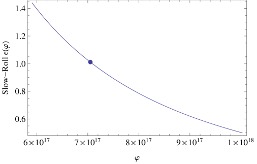
As we can see, the slow-roll condition is violated at the field value , which is indicated by a dot on the graph. Thus, in the single-scalar case the ending of slow roll is characterized by a single point in the corresponding phase space. This fact has a direct impact on the slow-roll parameter , as can be seen in Fig. 1.
Let us now come to the two-field case, which as we show is more involved. In order to simplify things we choose a simple example, and we consider the Hubble rate to be
| (3.43) |
with and being equal to
| (3.44) |
where and are parameters. In this case the Type IV singularity occurs if . Thus, we can accommodate the Type IV singularity in a generalized two-field scalar-tensor theory with action given in (2.32), by following the reconstruction method of the previous section, with chosen as in (3.5). In particular, the kinetic functions and are equal to
| (3.45) |
and by substituting the functions from (3.44) we acquire
| (3.46) |
Therefore, the corresponding scalar potential writes as
| (3.47) |
We assume that is identical with the cosmological time when inflation ends, and thus it is a very small number. In addition, we assume that inflation occurs for large field values, and thus at the time when inflation occurs, and . Since , the potential can be simplified to a great extent by keeping the dominant terms, becoming
| (3.48) |
As a next step, we can transform the above two-field scalar-tensor theory to one that contains only canonical scalar fields. Indeed, by making the transformation
| (3.49) |
we can extract the identifications
| (3.50) |
where and stand for
| (3.51) |
Hence, in terms of the canonical scalar fields and , the simplified scalar potential (3.48) reads
| (3.52) |
while the canonical two-field action is simply
| (3.53) |
Having the scalar potential (3.2) at hand, we can qualitatively investigate when the slow-roll approximation is violated. Practically this occurs when the slow-roll parameter becomes . In the case of a scalar-tensor theory with two canonical scalar fields, the slow-roll parameter is equal to [119, 120, 121, 122, 123, 124, 125, 126, 127]:
| (3.54) |
with and reading as
| (3.55) |
Thus, by using the potential (3.2) we may directly evaluate the slow-roll parameter and study it’s evolution as a function of the two scalar fields. Assuming again large field values for small cosmological times, which decrease as the cosmic time approaches the end of inflation, in Fig. 2 we present the behavior of the slow-roll parameter as a function of the scalar fields.
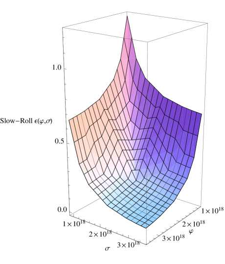
As we observe the slow-roll approximation is violated for a combination of values of the two fields, as expected.
Before closing this subsection, we shall investigate the impact of the singularities on the cosmological parameters of the two-field model. In particular, we are interested in the cases where the singularities may lead to inconsistencies. As we mentioned earlier, the main inconsistency is traced in the definition of the -fold number , which is defined as
| (3.56) |
where is the Hubble exit during inflation. The final time corresponds to a uniform-density hypersurface, at which inflation is considered to end. By taking into account (3.43) and (3.44), the folding number writes as
| (3.57) |
Hence, it is obvious that when the above expression is always singular when , due to the last term. However, if the singularity is of Type IV there is no inconsistency, which is the main point of this subsection.
Finally, as we mentioned earlier too, we note that the complete analysis of the -folding number for the two-field case can be quite complicated, and a detailed investigation would require the use of the N approximation. However, such a study stretches beyond the scope of the present work, and the reader is referred to [119, 120, 121, 122, 123, 124, 125, 126, 127] and references therein.
3.3 Singular inflation with singular dark energy
In this subsection we are interested in constructing a cosmological scenario where singular inflation gives rise to radiation and matter eras, and eventually to a dark energy epoch that results in a Big-Rip singularity. In order to succeed this, and following the previous subsections, we use two scalar fields, and thus this is another indication of the capabilities of such a model.
Having in mind the discussion on the singularity types of the Hubble rate (2.14), we deduce that a Hubble rate that captures the above features, namely a singular inflation with a type IV singularity and a dark energy epoch resulting to a Big Rip, writes as
| (3.58) |
where and , with , , constants, and where and are respectively the time of the inflationary type IV singularity and of the Big Rip. We need to note that is assumed to take values of (3.2), therefore complex values for the Hubble rate are avoided for the physically interesting interval . Practically, since the denominator of the fraction appearing in (3.2) is an odd integer always, then this procedure is always valid. Definitely, there are extra complex conjugate branches too, but we only focus on the real negative one.
Assuming as usual that the two scalar fields and depend only on the cosmic-time coordinate , and also that the spacetime is described by a flat FRW metric of the form (2.1), we extract the Friedmann equations in the form
| (3.59) | |||
| (3.60) |
Following the procedure of the previous subsections we impose the parametrization
| (3.61) |
which is consistent with the explicit solution of (3.59) and (3.60):
| (3.62) |
A convenient choice for the kinetic functions would be
| (3.63) |
with an arbitrary function of its argument. It proves useful to define a new function through
| (3.64) |
which has the characteristic property which fixes the constants of integration in (3.64). Assuming that is given in terms of the function as
| (3.65) |
we find that in addition to the Friedmann equations given in (3.59) and (3.60) we have
| (3.66) | |||
| (3.67) |
Hence, using the above kinetic functions , and the scalar potential we obtain a two-field scalar-tensor model with cosmological evolution of the form (3.58).
As a next step we need to impose an ansatz for the function appeared in (3.63). We choose it as
| (3.68) |
and therefore (3.63) give
| (3.69) |
As expected, one of the fields is canonical while the other one is ghost. The corresponding function from (3.64) becomes
| (3.70) |
and thus the scalar potential from (3.65) becomes
| (3.71) |
In summary, the above two-field model can give rise to the Hubble rate (3.58), which corresponds to a universe with a singular (of type IV) inflation, resulting in a dark-energy phase that ends with a Big Rip.
3.4 Barrow’s two-field model
In this subsection, for completeness, we present the realization of the singular inflation in the Barrow’s two-field model [74]. This model can exhibit the Type IV singularity consistently incorporated in it’s scalar-tensor theoretical framework. In particular, we consider a Hubble rate of the form
| (3.72) |
We choose the arbitrary function appearing in (2.37) to be
| (3.73) |
and substituting this into (2.37) we can easily obtain the corresponding kinetic functions and as
| (3.74) |
In the case at hand, and assuming that has the form (2.45), namely , with constrained to be an even integer and , the kinetic function is rendered positive, while the kinetic function becomes always negative. Thus, we can promptly find the function , which in this case is
| (3.75) |
and consequently the corresponding scalar potential reads
| (3.76) |
Therefore, the two-field scalar-tensor theory that generates the cosmological evolution of (3.72), is given by expressions (3.74) and (3.4).
3.5 The case of multiple scalar fields
We close the current section by presenting, for completeness, the possible generalization of the above results in the case of multiple fields. Such a framework offers huge capabilities and possibilities of cosmological evolutions. We provide here the general framework of this extension following [106] (see also [128]). The scalar-tensor action in the case of real scalar fields , , reads
| (3.77) |
Assuming a flat FRW background, and assuming that the scalar fields are functions only of the cosmic time , the corresponding Friedmann equations write as
| (3.78) | |||
| (3.79) |
We choose the function in order to satisfy the following equation:
| (3.80) |
and therefore we obtain
| (3.81) |
with the function . The solution of the reconstruction method is then given by
| (3.82) |
By appropriately choosing some arbitrary functions we can make the kinetic functions to be
| (3.83) | |||||
Hence, one may choose to have ghost and non-ghost scalar fields and describe the cosmological evolution in a desired way. We do not analyze this case in more details since it lies beyond the scope of the present work.
4 -gravity analysis
As a last section of this work, and for completeness, we will investigate the case of gravity [134, 104, 129, 130, 105, 101, 131, 132, 133], which is closely related to scalar-field theory, focusing again on the Type IV realization of a Hubble rate of the form (2.2). We will follow the reconstruction procedure of [135, 136, 137] (see also [69]).
We start by recalling that in the case where , the scalar-tensor potential which perfectly describes this cosmology is a hilltop-like potential of the form (2.13). We shall assume that the parameters and appearing in (2.14) are chosen in order to satisfy and , and in addition . Furthermore, we remind that for an FRW metric, the Ricci scalar writes as
| (4.1) |
As the cosmic time approaches the finite time , then . We shall use this property later on in this section, in order to find approximate expressions for the gravity. In addition, as , the Ricci scalar approaches the limiting value , as can be seen by calculating it’s analytic form
| (4.2) |
We shall further investigate the physical consequences of our assumptions in the end of this section.
The Jordan frame action of a pure gravity is
| (4.3) |
with pure referring to the absence of matter fluids. Varying action (4.3) with respect to the metric tensor leads to the Friedmann equation
| (4.4) |
By making use of an auxiliary scalar field (which has no kinetic term), the gravity action of (4.3) can be rewritten as
| (4.5) |
By finding the exact analytic form of the functions and , which have an explicit dependence on the scalar field , we may easily obtain the specific gravity. This can be done by varying the action of (4.5) with respect to the auxiliary scalar degree of freedom . Such a variation gives
| (4.6) |
with the prime now denoting differentiation with respect to . Solving Eq. (4.6) with respect to will provide us with the function , and then the gravity can be easily found by substituting to the auxiliary action of (4.5). Hence, the reconstructed gravity will be
| (4.7) |
Let us apply the above reconstruction procedure for the case where the Hubble rate is
| (4.8) |
By varying action (4.5) with respect to the metric, we obtain the equations
| (4.9) |
Eliminating from (4) results to
| (4.10) |
In this way, given the Hubble rate, the explicit form of can be found and from this we can obtain accordingly. We mention that, due to fact that the action (4.3) is mathematically equivalent to the auxiliary action (4.5), the auxiliary scalar field is identical to the cosmic time , that is . This was proven in detail in the Appendix A of Ref. [135]. Substituting the Hubble rate (4.8) in (4.10), we obtain the following second-order differential equation:
| (4.11) |
which by setting can be rewritten as
| (4.12) |
The general solution of the above equation is difficult to be extracted, thus we will follow approximations. In particular, since is small the differential equation becomes
| (4.13) |
with solution
| (4.14) |
with , being arbitrary constants. Then, the function can easily be calculated using (4) as
| (4.15) |
Substituting the final forms of the functions and into (4.6), and by solving with respect to , we can find the function . For the case that we are interested in, i.e. for , we can expand the involved and . Doing so we acquire
| (4.16) |
and
| (4.17) |
Since , keeping the most dominant terms in (4) we obtain
| (4.18) |
Hence, substituting (4.16) and (4.18) into (4.6) we acquire
| (4.19) |
Thus, the gravity form that can reproduce the Type IV singularity, can be obtained straightforwardly upon substitution of (4.19) into (4.7), and reads as
| (4.20) |
Observing the above form, we deduce that by appropriately choosing the arbitrary constant we can make the function to be the usual Einstein-Hilbert gravity plus curvature corrections. Indeed, for , the form becomes
| (4.21) |
We can further simplify the final form of the gravity by recalling that (4.21) is valid only near the Type IV singularity, in which case the Ricci scalar approaches the limiting value (see (4.2)). Therefore, for , the last two terms of (4.21) are nearly zero. Consequently, the final form of the gravity is approximately
| (4.22) |
This type of gravity was described in [101]. Recall our initial assumptions, namely and , and in addition . Furthermore, as the scalar curvature approaches the limiting value . Therefore, we have an appealing physical picture if we additionally require that is a future late-time singularity. Indeed, the gravity is of the form and the scalar curvature approaches a late-time point, which since this limiting curvature value can be chosen to have a very small value. Hence, the form of (4.22) can successfully describe late-time acceleration near the future Type IV singularity, which was the goal of the present section.
We mention that the gravity of the form (4.22) can consistently describe dark energy and late-time acceleration, as was demonstrated in [101], and with the presence of an term it can unify inflation with dark energy [138]. However, the model (4.22) is not completely in agreement with observations, having problems with the correct description of the gravitational interaction in the Solar System. Nevertheless, the model (4.22) turns out to be a very useful approximate form of consistent and realistic versions of gravity (see [133] for a review). However, we have to note that the de Sitter solution for this model is , thus for negative the model we found may not describe dark energy, as was shown in [139, 140], since . Additionally, as it was stressed in [141], in order for the scalaron mass to be less than the Planck mass, the has to be bounded for a finite , which is not satisfied by (4.20).
5 Conclusions
In this work we demonstrated that finite time singularities of Type IV, can consistently be incorporated in the Universe’s cosmological evolution, either appearing in the inflationary era, or in the late-time regime. We thoroughly discussed the most consistent framework in which these can be realized without instabilities. In particular, using only one scalar field then the linear-level instabilities can in principle occur at the cosmological time at which the phantom divide is crossed during the dynamical evolution, as we showed to happen in the case of a hilltop-like potential. On the other hand, when two fields are involved, one being canonical and one being ghost, it is possible to avoid such instabilities during the phantom-divide crossing. In addition, despite their increased level of complexity, the two-field scalar-tensor theories prove to be able to offer a plethora of possible viable cosmological scenarios, at which various types of cosmological singularities can be realized. For instance, it is possible to describe phantom inflation with the appearance of a Type IV singularity, and phantom late-time acceleration which ends in a Big Rip singularity.
For completeness, we also presented the Type IV realization in the context of gravity, which is known to be connected with a scalar-field theory through conformal transformations. In particular, we showed that specifically reconstructed forms can generate cosmological scenarios with a dynamical evolution corresponding to hilltop-like potentials. As we evinced, the resulting gravity is of the form , and this can be quite physically appealing if the Type IV singularity occurs at late times, since the resulting model is known to produce late-time acceleration.
In the absence of a complete understanding of the nature of cosmological singularities, we believe that with the present study we demonstrated that not all singularities can be harmful, at least for the cases where observational consistency is the main goal of a self-consistent physical theory. Indeed, even in observable quantities that contain higher derivatives of the scale factor, the effect of singularities, and particularly of Type IV singularities, might be negligible, as for example in the jerk parameter. Definitely, a lot of effort is needed to theoretically understand the singularities, but probably these Type IV singularities might be a classical bridge between classical cosmology and the ultimate quantum gravitational cosmology, which offers a complete description or at least a remedy of these classically unwanted spacetime points. Some steps towards these directions of research are offered by loop quantum gravity, in which no singularities occur [142, 143, 144, 145, 146]. However, we mention that it is possible even at the classical level to remedy singularities [23] or even avoid them [60], when quantum corrections are taken into account, as in [6, 23], and thus we hope to address this issue in the future in more details.
It would be interesting to notice that phantom-non-phantom transitions as well as non-singular evolution appear also in the case of bouncing cosmology. Hence, one could follow the procedures and the techniques of the present work, in order to investigate the effects of Type IV singularities, and probably of Type III ones, in the context of various ekpyrotic [147, 149, 148] or bounce Universe scenarios [29, 30, 31, 33, 32, 34, 35, 36, 37, 38, 39, 40, 41, 42, 45, 43, 44, 46, 47, 48, 49, 50]. This thorough analysis lies beyond the scope of the present work and will be addressed elsewhere.
Finally, we have to mention that in this work we did not address in general the issue of possible analyticity loss beyond . As it is also commented by Barrow and Graham in [74], for large-field inflation potentials of the form , there are fractional powers of for which the potential is always real, and extensibility through can be achieved leading to a Big Crunch (for instance when the potential becomes negative). The forms of the potentials we used are exactly of this class (large-field inflation ones), or hilltop-like potentials. Nevertheless, in general, the analyticity issue around is very interesting, both from mathematical as well as physical point of view. This issue however deserves a detailed investigation of its own and is left for a future project.
Acknowledgments
This work is supported in part by the JSPS Grant-in-Aid for Scientific Research (S) # 22224003 and (C) # 23540296 (S.N.) and in part by MINECO (Spain), projects FIS2010-15640 and FIS2013-44881. The research of ENS is implemented within the framework of the Action “Supporting Postdoctoral Researchers” of the Operational Program “Education and Lifelong Learning” (Actions Beneficiary: General Secretariat for Research and Technology), and is co-financed by the European Social Fund (ESF) and the Greek State.
References
- [1] S. Nojiri and S. D. Odintsov, Unifying phantom inflation with late-time acceleration: Scalar phantom-non-phantom transition model and generalized holographic dark energy, Gen. Rel. Grav. 38, 1285 (2006) [arXiv:hep-th/0506212].
- [2] S. Hannestad and E. Mortsell, Probing the dark side: Constraints on the dark energy equation of state from CMB, large scale structure and Type Ia supernovae, Phys. Rev. D 66, 063508 (2002) [arXiv:astro-ph/0205096].
- [3] H. K. Jassal, J. S. Bagla and T. Padmanabhan, Observational constraints on low redshift evolution of dark energy: How consistent are different observations?, Phys. Rev. D 72, 103503 (2005) [arXiv:astro-ph/0506748].
- [4] Y. F. Cai, E. N. Saridakis, M. R. Setare and J. Q. Xia, Quintom Cosmology: Theoretical implications and observations, Phys. Rept. 493, 1 (2010) [arXiv:0909.2776].
- [5] A. A. Starobinsky, Future and origin of our universe: Modern view, Grav. Cosmol. 6, 157 (2000) [arXiv:astro-ph/9912054].
- [6] E. Elizalde, S. Nojiri and S. D. Odintsov, Late-time cosmology in (phantom) scalar-tensor theory: Dark energy and the cosmic speed-up, Phys. Rev. D 70 (2004) 043539 [arXiv:hep-th/0405034].
- [7] R. R. Caldwell, A Phantom menace?, Phys. Lett. B 545, 23 (2002), [arXiv:astro-ph/9908168].
- [8] S. Nojiri and S. D. Odintsov, DeSitter brane universe induced by phantom and quantum effects, Phys. Lett. B 565, 1 (2003) [arXiv:hep-th/0304131].
- [9] V. Faraoni, Coupled oscillators as models of phantom and scalar field cosmologies, Phys. Rev. D 69, 123520 (2004) [arXiv:gr-qc/0404078].
- [10] P. Singh, M. Sami and N. Dadhich, Cosmological dynamics of phantom field, Phys. Rev. D 68, 023522 (2003) [arXiv:hep-th/0305110].
- [11] M. Sami and A. Toporensky, Phantom Field and the Fate of Universe, Mod. Phys. Lett. A 19, 1509 (2004) [arXiv:gr-qc/0312009].
- [12] P. F. Gonzalez-Diaz, K-essential phantom energy: Doomsday around the corner?, Phys. Lett. B 586, 1 (2004) [arXiv:astro-ph/0312579].
- [13] V. K. Onemli and R. P. Woodard, Quantum effects can render on cosmological scales, Phys. Rev. D 70, 107301 (2004) [arXiv:gr-qc/0406098].
- [14] V. Faraoni, Phantom cosmology with general potentials, Class. Quant. Grav. 22, 3235 (2005) [arXiv:gr-qc/0506095].
- [15] Z. K. Guo, Y. S. Piao, X. M. Zhang and Y. Z. Zhang, Cosmological evolution of a quintom model of dark energy, Phys. Lett. B 608, 177 (2005) [arXiv:astro-ph/0410654].
- [16] E. N. Saridakis, P. F. Gonzalez-Diaz and C. L. Siguenza, Unified dark energy thermodynamics: varying w and the -1-crossing, Class. Quant. Grav. 26, 165003 (2009) [arXiv:0901.1213].
- [17] B. Boisseau, G. Esposito-Farese, D. Polarski and A. A. Starobinsky, Reconstruction of a scalar tensor theory of gravity in an accelerating universe, Phys. Rev. Lett. 85, 2236 (2000) [arXiv:gr-qc/0001066].
- [18] A. Vikman, Can dark energy evolve to the phantom?, Phys. Rev. D 71, 023515 (2005) [arXiv:astro-ph/0407107].
- [19] Y. Ito, S. Nojiri and S. D. Odintsov, Stability of Accelerating Cosmology in Two Scalar-Tensor Theory: Little Rip versus de Sitter, Entropy 14 (2012) 1578 [arXiv:1111.5389].
- [20] S. Nojiri, S. D. Odintsov, V. K. Oikonomou, A quantitative analysis of singular inflation with scalar-tensor and modified gravity, [arXiv:1502.07005].
- [21] P. A. R. Ade et al. [Planck Collaboration], Planck 2013 results. XXII. Constraints on inflation, Astron. Astrophys. 571 (2014) A22 [arXiv:1303.5082].
- [22] P. A. R. Ade et al. [BICEP2 Collaboration], Detection of B-Mode Polarization at Degree Angular Scales by BICEP2, Phys. Rev. Lett. 112, 241101 (2014) [arXiv:1403.3985].
- [23] S. Nojiri, S. D. Odintsov and S. Tsujikawa, Properties of singularities in (phantom) dark energy universe, Phys. Rev. D 71, 063004 (2005) [arXiv:hep-th/0501025].
- [24] S. W. Hawking and R. Penrose, The Singularities of gravitational collapse and cosmology, Proc. Roy. Soc. Lond. A 314 (1970) 529.
- [25] V. Mukhanov, Physical foundations of cosmology, Cambridge, UK: Univ. Pr. (2005) 421 p.
- [26] D. S. Gorbunov and V. A. Rubakov, Introduction to the theory of the early universe: Cosmological perturbations and inflationary theory, Hackensack, USA: World Scientific (2011) 489 p.
- [27] A. Linde, Inflationary Cosmology after Planck 2013, [arXiv:1402.0526].
- [28] D. H. Lyth and A. Riotto, Particle physics models of inflation and the cosmological density perturbation, Phys. Rept. 314 (1999) 1 [arXiv:hep-ph/9807278].
- [29] A.A. Starobinsky On a nonsingular isotropic cosmological model, Sov. Astron. Lett. 4(2), 82-84 (1978).
- [30] M. Novello and S. E. P. Bergliaffa, Bouncing Cosmologies, Phys. Rept. 463, 127 (2008), [arXiv:0802.1634].
- [31] R. H. Brandenberger, V. F. Mukhanov and A. Sornborger, A Cosmological theory without singularities, Phys. Rev. D 48, 1629 (1993), [arXiv:gr-qc/9303001].
- [32] Y. F. Cai, D. A. Easson and R. Brandenberger, Towards a Nonsingular Bouncing Cosmology, JCAP 1208, 020 (2012) [arXiv:1206.2382].
- [33] J. Khoury, B. A. Ovrut and J. Stokes, The Worldvolume Action of Kink Solitons in AdS Spacetime, JHEP 1208, 015 (2012) [arXiv:1203.4562].
- [34] T. Qiu, X. Gao and E. N. Saridakis, Towards anisotropy-free and nonsingular bounce cosmology with scale-invariant perturbations, Phys. Rev. D 88, no. 4, 043525 (2013) [arXiv:1303.2372].
- [35] Y. F. Cai, J. Quintin, E. N. Saridakis and E. Wilson-Ewing, Nonsingular bouncing cosmologies in light of BICEP2, JCAP 1407, 033 (2014) [arXiv:1404.4364].
- [36] J. Khoury, B. A. Ovrut, P. J. Steinhardt and N. Turok, Density perturbations in the ekpyrotic scenario, Phys. Rev. D 66, 046005 (2002) [arXiv:hep-th/0109050].
- [37] J. K. Erickson, D. H. Wesley, P. J. Steinhardt and N. Turok, Kasner and mixmaster behavior in universes with equation of state w ¿= 1, Phys. Rev. D 69, 063514 (2004) [arXiv:hep-th/0312009].
- [38] J. L. Lehners and P. J. Steinhardt, Planck 2013 results support the cyclic universe, Phys. Rev. D 87, no. 12, 123533 (2013) [arXiv:1304.3122].
- [39] E. N. Saridakis, Cyclic Universes from General Collisionless Braneworld Models, Nucl. Phys. B 808, 224 (2009), [arXiv:0710.5269].
- [40] P. Creminelli and L. Senatore, A Smooth bouncing cosmology with scale invariant spectrum, JCAP 0711, 010 (2007) [arXiv:hep-th/0702165].
- [41] Y. -F. Cai and E. N. Saridakis, Cyclic cosmology from Lagrange-multiplier modified gravity, Class. Quant. Grav. 28, 035010 (2011), [arXiv:1007.3204].
- [42] R. Brandenberger, Matter Bounce in Horava-Lifshitz Cosmology, Phys. Rev. D 80, 043516 (2009), [arXiv:0904.2835].
- [43] J. Martin and P. Peter, Parametric amplification of metric fluctuations through a bouncing phase, Phys. Rev. D 68, 103517 (2003), [arXiv:hep-th/0307077].
- [44] Y. F. Cai, C. Gao and E. N. Saridakis, Bounce and cyclic cosmology in extended nonlinear massive gravity, JCAP 1210 (2012) 048 [arXiv:1207.3786].
- [45] M. Bojowald, Absence of singularity in loop quantum cosmology, Phys. Rev. Lett. 86, 5227 (2001) [arXiv:gr-qc/0102069].
- [46] A. Ashtekar, An Introduction to Loop Quantum Gravity Through Cosmology, Nuovo Cim. B 122, 135 (2007) [arXiv:gr-qc/0702030].
- [47] T. Cailleteau, A. Barrau, J. Grain and F. Vidotto, Consistency of holonomy-corrected scalar, vector and tensor perturbations in Loop Quantum Cosmology, Phys. Rev. D 86, 087301 (2012) [arXiv:1206.6736].
- [48] J. Haro and J. Amoros, Viability of the matter bounce scenario in Loop Quantum Cosmology for general potentials, JCAP(12) 031 (2014) [arXiv:1406.0369].
- [49] J. Amoros, J. de Haro and S. D. Odintsov, Loop Quantum Cosmology, Phys. Rev. D 89, no. 10, 104010 (2014) [arXiv:1402.3071].
- [50] E. Wilson-Ewing, The Matter Bounce Scenario in Loop Quantum Cosmology, JCAP 1303, 026 (2013) [arXiv:1211.6269].
- [51] J. D. Barrow, Sudden future singularities, Class. Quant. Grav. 21 (2004) L79 [arXiv:gr-qc/0403084].
- [52] Y. Shtanov and V. Sahni, Unusual cosmological singularities in brane world models, Class. Quant. Grav. 19 (2002) L101 [arXiv:gr-qc/0204040].
- [53] V. Gorini, A. Y. Kamenshchik, U. Moschella and V. Pasquier, Tachyons, scalar fields and cosmology, Phys. Rev. D 69, 123512 (2004) [arXiv:hep-th/0311111].
- [54] J. D. Barrow, More general sudden singularities, Class. Quant. Grav. 21 (2004) 5619 [arXiv:gr-qc/0409062].
- [55] K. Lake, Sudden future singularities in FLRW cosmologies, Class. Quant. Grav. 21, L129 (2004) [arXiv:gr-qc/0407107].
- [56] S. Cotsakis and I. Klaoudatou, Future singularities of isotropic cosmologies, J. Geom. Phys. 55, 306 (2005) [arXiv:gr-qc/0409022].
- [57] M. P. Dabrowski, Inhomogenized sudden future singularities, Phys. Rev. D 71, 103505 (2005) [arXiv:gr-qc/0410033].
- [58] L. Fernandez-Jambrina and R. Lazkoz, Geodesic behaviour of sudden future singularities, Phys. Rev. D 70, 121503 (2004) [arXiv:gr-qc/0410124].
- [59] J. D. Barrow and C. G. Tsagas, New isotropic and anisotropic sudden singularities, Class. Quant. Grav. 22, 1563 (2005) [arXiv:gr-qc/0411045].
- [60] S. Nojiri and S. D. Odintsov, Quantum escape of sudden future singularity, Phys. Lett. B 595, 1 (2004) [arXiv:hep-th/0405078].
- [61] H. Stefancic, Expansion around the vacuum equation of state - Sudden future singularities and asymptotic behavior, Phys. Rev. D 71, 084024 (2005) [arXiv:gr-qc/0411630].
- [62] S. Nojiri and S. D. Odintsov, The Final state and thermodynamics of dark energy universe, Phys. Rev. D 70 (2004) 103522 [arXiv:hep-th/0408170].
- [63] S. Nojiri and S. D. Odintsov, Inhomogeneous equation of state of the universe: Phantom era, future singularity and crossing the phantom barrier, Phys. Rev. D 72, 023003 (2005) [arXiv:hep-th/0505215].
- [64] C. Cattoen and M. Visser, Necessary and sufficient conditions for big bangs, bounces, crunches, rips, sudden singularities, and extremality events, Class. Quant. Grav. 22, 4913 (2005) [arXiv:gr-qc/0508045].
- [65] M. Sami, P. Singh and S. Tsujikawa, Avoidance of future singularities in loop quantum cosmology, Phys. Rev. D 74, 043514 (2006) [arXiv:gr-qc/0605113].
- [66] M. Bouhmadi-Lopez, P. F. Gonzalez-Diaz and P. Martin-Moruno, Worse than a big rip?, Phys. Lett. B 659, 1 (2008) [arXiv:gr-qc/0612135].
- [67] A. V. Yurov, A. V. Astashenok and P. F. Gonzalez-Diaz, Astronomical bounds on future big freeze singularity, Grav. Cosmol. 14, 205 (2008) [arXiv:0705.4108].
- [68] L. Fernandez-Jambrina and R. Lazkoz, Singular fate of the universe in modified theories of gravity, Phys. Lett. B 670, 254 (2009) [arXiv:0805.2284].
- [69] K. Bamba, S. Nojiri and S. D. Odintsov, The Universe future in modified gravity theories: Approaching the finite-time future singularity, JCAP 0810 (2008) 045 [arXiv:0807.2575].
- [70] J. D. Barrow and S. Z. W. Lip, The Classical Stability of Sudden and Big Rip Singularities, Phys. Rev. D 80, 043518 (2009) [arXiv:0901.1626].
- [71] M. Bouhmadi-Lopez, C. Kiefer, B. Sandhofer and P. V. Moniz, On the quantum fate of singularities in a dark-energy dominated universe, Phys. Rev. D 79, 124035 (2009) [arXiv:0905.2421].
- [72] K. Bamba, S. D. Odintsov, L. Sebastiani and S. Zerbini, Finite-time future singularities in modified Gauss-Bonnet and F(R,G) gravity and singularity avoidance, Eur. Phys. J. C 67, 295 (2010) [arXiv:0911.4390].
- [73] J. D. Barrow, S. Cotsakis and A. Tsokaros, A General Sudden Cosmological Singularity, Class. Quant. Grav. 27, 165017 (2010) [arXiv:1004.2681].
- [74] J. D. Barrow and A. A. H. Graham, Singular Inflation, [arXiv:1501.04090].
- [75] R. R. Caldwell, M. Kamionkowski and N. N. Weinberg, Phantom Energy and Cosmic Doomsday, Phys. Rev. Lett. 91, 071301 (2003) [arXiv:astro-ph/0302506].
- [76] B. McInnes, The dS/CFT correspondence and the big smash, JHEP 0208 (2002) 029 [arXiv:hep-th/0112066].
- [77] V. Faraoni, Superquintessence, Int. J. Mod. Phys. D 11, 471 (2002) [arXiv:astro-ph/0110067].
- [78] V. Gorini, A. Kamenshchik and U. Moschella, Can the Chaplygin gas be a plausible model for dark energy?, Phys. Rev. D 67, 063509 (2003) [arXiv:astro-ph/0209395].
- [79] L. P. Chimento and R. Lazkoz, On the link between phantom and standard cosmologies, Phys. Rev. Lett. 91, 211301 (2003) [arXiv:gr-qc/0307111].
- [80] H. Stefancic, Generalized phantom energy, Phys. Lett. B 586, 5 (2004) [arXiv:astro-ph/0310904].
- [81] L. P. Chimento and R. Lazkoz, On big rip singularities, Mod. Phys. Lett. A 19, 2479 (2004) [arXiv:gr-qc/0405020].
- [82] C. Csaki, N. Kaloper and J. Terning, Exorcising , Annals Phys. 317, 410 (2005) [arXiv:astro-ph/0409596].
- [83] J. G. Hao and X. Z. Li, Generalized quartessence cosmic dynamics: Phantom or quintessence with de Sitter attractor, Phys. Lett. B 606, 7 (2005) [arXiv:astro-ph/0404154].
- [84] P. X. Wu and H. W. Yu, Avoidance of Big Rip In Phantom Cosmology by Gravitational Back Reaction, Nucl. Phys. B 727, 355 (2005) [arXiv:astro-ph/0407424].
- [85] M. P. Dabrowski and T. Stachowiak, Phantom Friedmann cosmologies and higher-order characteristics of expansion, Annals Phys. 321, 771 (2006) [arXiv:hep-th/0411199].
- [86] I. Y. Aref’eva, A. S. Koshelev and S. Y. Vernov, Exactly Solvable SFT Inspired Phantom Model, Theor. Math. Phys. 148, 895 (2006) [Teor. Mat. Fiz. 148, 23 (2006)] [arXiv:astro-ph/0412619].
- [87] X. F. Zhang, H. Li, Y. S. Piao and X. M. Zhang, Two-field models of dark energy with equation of state across -1, Mod. Phys. Lett. A 21, 231 (2006) [arXiv:astro-ph/0501652].
- [88] E. Elizalde, S. Nojiri, S. D. Odintsov and P. Wang, Dark energy: Vacuum fluctuations, the effective phantom phase, and holography, Phys. Rev. D 71, 103504 (2005) [arXiv:hep-th/0502082].
- [89] R. G. Cai, H. S. Zhang and A. Wang, Crossing w = -1 in Gauss-Bonnet brane world with induced gravity, Commun. Theor. Phys. 44, 948 (2005) [arXiv:hep-th/0505186].
- [90] F. S. N. Lobo, Phantom energy traversable wormholes, Phys. Rev. D 71, 084011 (2005) [arXiv:gr-qc/0502099].
- [91] J. Sola and H. Stefancic, Effective equation of state for dark energy: mimicking quintessence and phantom energy through a variable Lambda, Phys. Lett. B 624, 147 (2005) [arXiv:astro-ph/0505133].
- [92] E. M. Barbaoza and N. A. Lemos, Does the Big Rip survive quantization?, [arXiv:gr-qc/0606084].
- [93] A. Albrecht and P. J. Steinhardt, Cosmology for Grand Unified Theories with Radiatively Induced Symmetry Breaking, Phys. Rev. Lett. 48 (1982) 1220.
- [94] A. D. Linde, A New Inflationary Universe Scenario: A Possible Solution of the Horizon, Flatness, Homogeneity, Isotropy and Primordial Monopole Problems, Phys. Lett. B 108, 389 (1982).
- [95] K. Kohri, C. M. Lin and D. H. Lyth, More hilltop inflation models, JCAP 0712, 004 (2007) [arXiv:0707.3826].
- [96] S. Dutta and R. J. Scherrer, Hilltop Quintessence, Phys. Rev. D 78, 123525 (2008) [arXiv:0809.4441].
- [97] S. Dutta, E. N. Saridakis and R. J. Scherrer, Dark energy from a quintessence (phantom) field rolling near potential minimum (maximum), Phys. Rev. D 79, 103005 (2009) [arXiv:0903.3412].
- [98] A. Ijjas, P. J. Steinhardt and A. Loeb, Inflationary paradigm in trouble after Planck2013, Phys. Lett. B 723, 261 (2013) [arXiv:1304.2785].
- [99] S. Antusch, D. Nolde and S. Orani, Hilltop inflation with preinflation from coupling to matter fields, JCAP 1405, 034 (2014) [arXiv:1402.5328].
- [100] L. Boubekeur and D. H. Lyth, Hilltop inflation, JCAP 0507, 010 (2005) [arXiv:hep-ph/0502047].
- [101] S. M. Carroll, V. Duvvuri, M. Trodden and M. S. Turner, Is cosmic speed - up due to new gravitational physics?, Phys. Rev. D 70, 043528 (2004) [arXiv:astro-ph/0306438].
- [102] S. Capozziello, S. Nojiri and S. D. Odintsov, Unified phantom cosmology: inflation, dark energy and dark matter under the same standard, Phys. Lett. B 632, 597 (2006) [arXiv:hep-th/0507182].
- [103] V. Sahni and A. Starobinsky, Int. J. Mod. Phys. D 15 (2006) 2105 [arXiv:astro-ph/0610026].
- [104] S. Nojiri and S. D. Odintsov, Introduction to modified gravity and gravitational alternative for dark energy, eConf C 0602061 (2006) 06 [Int. J. Geom. Meth. Mod. Phys. 4 (2007) 115] [arXiv:hep-th/0601213].
- [105] A. de la Cruz-Dombriz and D. Saez-Gomez, Black holes, cosmological solutions, future singularities, and their thermodynamical properties in modified gravity theories, Entropy 14 (2012) 1717 [arXiv:1207.2663].
- [106] E. Elizalde, S. Nojiri, S. D. Odintsov, D. Saez-Gomez and V. Faraoni, Reconstructing the universe history, from inflation to acceleration, with phantom and canonical scalar fields, Phys. Rev. D 77 (2008) 106005 [arXiv:0803.1311].
- [107] J. D. Barrow, G. J. Galloway and F. J. Tipler, The closed-universe recollapse conjecture, Mon. Not. Roy. Astron. Soc. 223, 835 (1986).
- [108] J. M. Cline, S. Jeon and G. D. Moore, The Phantom menaced: Constraints on low-energy effective ghosts, Phys. Rev. D 70 (2004) 043543 [arXiv:hep-ph/0311312].
- [109] S. Nojiri and E. N. Saridakis, Phantom without ghost, Astrophys. Space Sci. 347, 221 (2013) [arXiv:1301.2686].
- [110] A. G. Muslimov, On the Scalar Field Dynamics in a Spatially Flat Friedman Universe, Class. Quant. Grav. 7, 231 (1990).
- [111] D. S. Salopek and J. R. Bond, Nonlinear evolution of long wavelength metric fluctuations in inflationary models, Phys. Rev. D 42, 3936 (1990).
- [112] E. J. Copeland, A. R. Liddle and D. Wands, Exponential potentials and cosmological scaling solutions, Phys. Rev. D 57, 4686 (1998) [arXiv:gr-qc/971106].
- [113] X. -m. Chen, Y. -g. Gong and E. N. Saridakis, Phase-space analysis of interacting phantom cosmology, JCAP 0904, 001 (2009) [arXiv:0812.1117].
- [114] G. Leon and C. R. Fadragas, Cosmological Dynamical Systems, LAP LAMBERT Academic Publishing, Saarbrücken (2011) [arXiv:1412.5701].
- [115] J. Q. Xia, Y. F. Cai, T. T. Qiu, G. B. Zhao and X. Zhang, Constraints on the Sound Speed of Dynamical Dark Energy, Int. J. Mod. Phys. D 17, 1229 (2008) [arXiv:astro-ph/0703202].
- [116] S. Nojiri and S. D. Odintsov, Quantum deSitter cosmology and phantom matter, Phys. Lett. B 562, 147 (2003) [arXiv:hep-th/0303117].
- [117] T. Damour and V. F. Mukhanov, Inflation without slow roll, Phys. Rev. Lett. 80, 3440 (1998) [arXiv:gr-qc/9712061].
- [118] S. A. Appleby, R. A. Battye and A. A. Starobinsky, Curing singularities in cosmological evolution of F(R) gravity, JCAP 1006, 005 (2010) [arXiv:0909.1737].
- [119] A. A. Starobinsky, Multicomponent de Sitter (Inflationary) Stages and the Generation of Perturbations JETP Lett. 42 (1985) 152.
- [120] M. Sasaki and E. D. Stewart, A General analytic formula for the spectral index of the density perturbations produced during inflation Prog. Theor. Phys. 95 (1996) 71 [arXiv:astro-ph/9507001].
- [121] A. A. Starobinsky and L. A. Kofman, Effect of the cosmological constant on large-scale anisotropies in the microwave background, Sov. Astron. Lett., 11(5), 271-274 (1985).
- [122] D. H. Lyth and Y. Rodriguez, The Inflationary prediction for primordial non-Gaussianity Phys. Rev. Lett. 95 (2005) 121302 [arXiv:astro-ph/0504045].
- [123] F. Vernizzi and D. Wands, Non-gaussianities in two-field inflation, JCAP 0605 (2006) 019 [arXiv:astro-ph/0603799].
- [124] K. Y. Choi, L. M. H. Hall and C. van de Bruck, Spectral Running and Non-Gaussianity from Slow-Roll Inflation in Generalised Two-Field Models, JCAP 0702 (2007) 029 [arXiv:astro-ph/0701247].
- [125] L. Alabidi and D. H. Lyth, Inflation models after WMAP year three, JCAP 0608, 013 (2006) [arXiv:astro-ph/0603539].
- [126] L. Alabidi and D. H. Lyth, Inflation models and observation, JCAP 0605, 016 (2006) [arXiv:astro-ph/0510441].
- [127] M. Sasaki and T. Tanaka, Superhorizon scale dynamics of multiscalar inflation, Prog. Theor. Phys. 99 (1998) 763 [arXiv:gr-qc/9801017].
- [128] M. R. Setare and E. N. Saridakis, Quintom model with O(N) symmetry, JCAP 0809, 026 (2008) [arXiv:0809.0114].
- [129] V. Faraoni and S. Capozziello, Beyond Einstein gravity : A Survey of gravitational theories for cosmology and astrophysics, Fundamental Theories of Physics, Vol. 170, Springer, 2010.
- [130] S. Capozziello and M. De Laurentis, Extended Theories of Gravity, Phys. Rept. 509 (2011) 167 [arXiv:1108.6266].
- [131] S. Capozziello, Curvature quintessence, Int. J. Mod. Phys. D 11, 483 (2002) [arXiv:gr-qc/0201033].
- [132] S. Capozziello, V. F. Cardone and A. Troisi, Reconciling dark energy models with f(R) theories, Phys. Rev. D 71, 043503 (2005) [arXiv:astro-ph/0501426].
- [133] S. Nojiri and S. D. Odintsov, Unified cosmic history in modified gravity: from F(R) theory to Lorentz non-invariant models, Phys. Rept. 505 (2011) 59 [arXiv:1011.0544].
- [134] A. A. Starobinsky, A New Type of Isotropic Cosmological Models Without Singularity, Phys. Lett. B 91, 99 (1980).
- [135] S. Nojiri and S. D. Odintsov, Modified f(R) gravity consistent with realistic cosmology: From matter dominated epoch to dark energy universe, Phys. Rev. D 74, 086005 (2006) [arXiv:hep-th/0608008].
- [136] S. Capozziello, S. Nojiri, S. D. Odintsov and A. Troisi, Cosmological viability of f(R)-gravity as an ideal fluid and its compatibility with a matter dominated phase, Phys. Lett. B 639, 135 (2006) [arXiv:astro-ph/0604431].
- [137] S. Nojiri and S. D. Odintsov, Modified gravity and its reconstruction from the universe expansion history, J. Phys. Conf. Ser. 66, 012005 (2007) [arXiv:hep-th/0611071].
- [138] S. Nojiri, S. D. Odintsov, Modified gravity with negative and positive powers of the curvature: Unification of the inflation and of the cosmic acceleration, Phys. Rev. D 68 (2003) 123512 [arXiv:hep-th/0307288].
- [139] L. Amendola, D. Polarski and S. Tsujikawa, Are f(R) dark energy models cosmologically viable ?, Phys. Rev. Lett. 98 (2007) 131302 [arXiv:astro-ph/0603703].
- [140] L. Amendola, R. Gannouji, D. Polarski and S. Tsujikawa, Conditions for the cosmological viability of f(R) dark energy models, Phys. Rev. D 75 (2007) 083504 [arXiv:gr-qc/0612180].
- [141] A. A. Starobinsky, Disappearing cosmological constant in f(R) gravity, JETP Lett. 86 (2007) 157 [arXiv:0706.2041].
- [142] A. Ashtekar and P. Singh, Loop Quantum Cosmology: A Status Report, Class. Quant. Grav. 28 (2011) 213001 [arXiv:1108.0893].
- [143] M. Bojowald, Consistent Loop Quantum Cosmology, Class. Quant. Grav. 26 (2009) 075020 [arXiv:0811.4129].
- [144] J. Quintin, Y. F. Cai and R. H. Brandenberger, Matter creation in a nonsingular bouncing cosmology, Phys. Rev. D 90 (2014) 6, 063507 [arXiv:1406.6049].
- [145] J. de Haro, Does loop quantum cosmology replace the big rip singularity by a non-singular bounce?, JCAP 1211, 037 (2012) [arXiv:1207.3621].
- [146] Y. F. Cai, R. Brandenberger and X. Zhang, The Matter Bounce Curvaton Scenario, JCAP 1103, 003 (2011) [arXiv:1101.0822].
- [147] J. Khoury, B. A. Ovrut, P. J. Steinhardt and N. Turok, The ekpyrotic universe: Colliding branes and the origin of the hot big bang, Phys. Rev. D 64, 123522 (2001), [arXiv:hep-th/0103239].
- [148] J. L. Lehners, Ekpyrotic and Cyclic Cosmology, Phys. Rept. 465, 223 (2008) [arXiv:0806.1245].
- [149] J. Khoury, B. A. Ovrut, N. Seiberg, P. J. Steinhardt and N. Turok, From big crunch to big bang, Phys. Rev. D 65, 086007 (2002) [arXiv:hep-th/0108187].