Strong-majority bootstrap percolation on regular graphs with low dissemination threshold

Abstract

Consider the following model of strong-majority bootstrap percolation on a graph. Let $r\geq 1$ be some integer, and $p\in[0,1]$. Initially, every vertex is active with probability $p$, independently from all other vertices. Then, at every step of the process, each vertex $v$ of degree $\deg(v)$ becomes active if at least $(\deg(v)+r)/2$ of its neighbours are active. Given any arbitrarily small $p>0$ and any integer $r$, we construct a family of $d=d(p,r)$-regular graphs such that with high probability all vertices become active in the end. In particular, the case $r=1$ answers a question and disproves a conjecture of Rapaport, Suchan, Todinca, and Verstraëte [20].

1 Introduction

Given a graph $G=(V,E)$, a set $A\subseteq V$, and $j\in\mathbb{N}$, the bootstrap percolation process $\mathbb{B}_{j}(G;A)$ is defined as follows: initially, a vertex $v\in V$ is active if $v\in A$, and inactive otherwise. Then, at each round, each inactive vertex becomes active if it has at least $j$ active neighbours. The process keeps going until it reaches a stationary state in which every inactive vertex has less than $j$ active neighbours. We call this the final state of the process. Note that we may slow down the process by delaying the activation of some vertices, but the final state is invariant. If $G$ is a $d$-regular graph, then there is a natural characterization of the final state in terms of the $k$-core (i.e., the largest subgraph of minimum degree at least $k$): the set of inactive vertices in the final state of $\mathbb{B}_{j}(G;A)$ is precisely the vertex set of the $(d-j+1)$-core of the subgraph of $G$ induced by the initial set of inactive vertices $V\setminus A$ (see e.g. [14]). We say that $\mathbb{B}_{j}(G;A)$ disseminates if all vertices are active in the final state.

Define $\mathbb{B}_{j}(G;p)$ to be the same bootstrap percolation process, where the set of initially active vertices is chosen at random: each $v\in V$ is initially active with probability $p$, independently from all other vertices. This process (which can be regarded as a type of cellular automaton on graphs) was introduced in 1979 by Chalupa, Leath and Reich [9] on the grid $\mathbb{Z}^{m}$ as a simple model of dynamics of ferromagnetism, and has been widely studied ever since on many families of deterministic or random graphs. The following obvious monotonicity properties hold: for any $A^{\prime}\subseteq A^{\prime\prime}\subseteq V$, if $\mathbb{B}_{j}(G;A^{\prime})$ disseminates, then $\mathbb{B}_{j}(G;A^{\prime\prime})$ disseminates as well; similarly, if $i\leq j$ and $\mathbb{B}_{j}(G;A)$ disseminates, then $\mathbb{B}_{i}(G;A)$ must also disseminate. Therefore, the probability that $\mathbb{B}_{j}(G;p)$ disseminates is non-increasing in $j$ and non-decreasing in $p$. In view of this, one may expect that, for some sequences of graphs $G_{n}$, there may be a sharp probability threshold ${\widehat{p}}_{n}$ such that: for every constant $\varepsilon>0$, a.a.s. $\mathbb{B}_{j}(G_{n};p_{n})$ disseminates, if $p_{n}\geq(1+\varepsilon){\widehat{p}}_{n}$; and a.a.s. it does not disseminate, if $p_{n}\leq(1-\varepsilon){\widehat{p}}_{n}$. If such a value ${\widehat{p}}_{n}$ exists, we call it a dissemination threshold of $\mathbb{B}_{j}(G_{n};p_{n})$. Moreover, if $\lim_{n\to\infty}{\widehat{p}}_{n}={\widehat{p}}\in[0,1]$ exists, we call this limit ${\widehat{p}}$ the critical probability for dissemination, which is non-trivial if $0<{\widehat{p}}<1$. A lot of work has been done to establish dissemination thresholds or related properties of this process for different graph classes. In particular, denoting $\{1,2,\ldots,n\}$ by $[n]$, the case of $G$ being the $m$-dimensional grid $[n]^{m}$ has been extensively studied: starting with the work of Holroyd [13] analyzing the $2$-dimensional grid, the results then culminated in [5], where Balogh et al. gave precise and sharp thresholds for the dissemination of $\mathbb{B}_{j}([n]^{m};p)$ for any constant dimension $m\geq 2$ and every $2\leq j\leq m$. Other graph classes that have been studied are trees, hypercubes and hyperbolic lattices (see e.g. [7, 4, 6, 22]).

In the context of random graphs, Janson et al. [15] considered the model $\mathbb{B}_{j}(G;A)$ with $j\geq 2$, $G=\mathscr{G}(n,p)$ and $A$ being a set of vertices chosen at random from all sets of size $a(n)$. They showed a sharp threshold with respect to the parameter $a(n)$ that separates two regimes in which the final set of active vertices has a.a.s.  size $o(n)$ or $n-o(n)$ (i.e. ‘almost’ dissemination), respectively. Moreover, there is full dissemination in the supercritical regime provided that $\mathscr{G}(n,p)$ has minimum degree at least $j$. Balogh and Pittel [8] analysed the bootstrap percolation process on random $d$-regular graphs, and established non-trivial critical probabilities for dissemination for all $2\leq j\leq d-1$, and Amini [2] considered random graphs with more general degree sequences. Finally, extensions to inhomogeneous random graphs were considered by Amini, Fountoulakis and Panagiotou in [3].

Aside from its mathematical interest, bootstrap percolation was extensively studied by physicists: it was used to describe complex phenomena in jamming transitions [25], magnetic systems [21] and neuronal activity [24], and also in the context of stochastic Ising models [11]. For more applications of bootstrap percolation, see the survey [1] and the references therein.

Strong-majority model.

In this paper, we introduce a natural variant of the bootstrap percolation process. Given a graph $G=(V,E)$, an initially active set $A\subseteq V$, and $r\in\mathbb{Z}$, the $r$-majority bootstrap percolation process $\mathbb{M}_{r}(G;A)$ is defined as follows: starting with an initial set of active vertices $A$, at each round, each inactive vertex becomes active if the number of its active neighbours minus the number of its inactive neighbours is at least $r$. In other words, the activation rule for an inactive vertex $v$ of degree $\deg(v)$ is that $v$ has at least $\lceil(\deg(v)+r)/2\rceil$ active neighbours. As in ordinary bootstrap percolation, we are mainly interested in characterising the set of inactive vertices in the final state of and determining whether it is empty (i.e. the process disseminates) or not. Note that for a $d$-regular graph $G$, $\mathbb{M}_{r}(G;A)$ is exactly the same process as $\mathbb{B}_{\lceil(d+r)/2\rceil}(G;A)$, and therefore the final set of inactive vertices of $\mathbb{M}_{r}(G;A)$ is precisely the vertex set of the $\lfloor(d-r)/2+1\rfloor$-core of the graph induced by the initial set of inactive vertices. If $G$ is not regular, the two models are not comparable. The process $\mathbb{M}_{r}(G;p)$ is defined analogously for a random initial set $A$ of active vertices, where each vertex belongs to $A$ (i.e. is initially active) with probability $p$ and independently of all other vertices. Note that $\mathbb{M}_{r}(G;A)$ and $\mathbb{M}_{r}(G;p)$ satisfy the same monotonicity properties with respect to $A$, to $r$, and to $p$ that we described above for ordinary bootstrap percolation, and thus we define the critical probability ${\widehat{p}}$ for dissemination (if it exists) analogously as before. Additionally, for any (random or deterministic) sequence of graphs $G_{n}$, define

$${{\widehat{p}}\,^{+}} =\inf\{p\in[0,1]:\text{a.a.s.\ $\mathbb{M}_{r}(G_{n};p)$ disseminates}\}\qquad\text{and}$$

$${{\widehat{p}}\,^{-}} =\sup\{p\in[0,1]:\text{a.a.s.\ $\mathbb{M}_{r}(G_{n};p)$ does not disseminate}\}.$$

Trivially, $0\leq{{\widehat{p}}\,^{-}}\leq{{\widehat{p}}\,^{+}}\leq 1$; and, in case of equality, the critical probability ${\widehat{p}}$ must exist and satisfy ${\widehat{p}}={{\widehat{p}}\,^{-}}={{\widehat{p}}\,^{+}}$. The $r$-majority bootstrap percolation process is a generalisation of the non-strict majority and strict majority bootstrap percolation models, which correspond to the cases $r=0$ and $r=1$, respectively. The study of these two particular cases has received a lot of attention recently. For instance, Balogh, Bollobás and Morris [6] obtained the critical probability ${\widehat{p}}=1/2$ for the non-strict majority bootstrap percolation process $\mathbb{M}_{0}(G;p)$ on the hypercube $[2]^{n}$, and extended their results to the $m$-dimensional grid $[n]^{m}$ for $m\geq(\log\log n)^{2}(\log\log\log n)$. Also, Stefánsson and Vallier [23] studied the non-strict majority model for the random graph $\mathscr{G}(n,p)$. (Note that, since $\mathscr{G}(n,p)$ is not a regular graph, this process cannot be formulated in terms of ordinary bootstrap percolation). For the strict majority case, we first state a consequence of the work of Balogh and Pittel [8] on random $d$-regular graphs mentioned earlier. Let $\mathscr{G}_{n,d}$ denote a graph chosen uniformly at random (u.a.r. for short) from the set of all $d$-regular graphs on $n$ vertices (note that $n$ is even if $d$ is odd). Then, for any constant $d\geq 3$, the critical probability for dissemination of the process $\mathbb{M}_{1}(\mathscr{G}_{n,d};p)$ is equal to

$${\widehat{p}}(d):=1-\inf_{y\in(0,1)}\frac{y}{F(d-1,1-y)},$$ (1)

where $F(d,y)$ is the probability of obtaining at most $d/2$ successes in $d$ independent trials with success probability equal to $y$. Moreover,

$${\widehat{p}}(3)=1/2,\qquad\min\{{\widehat{p}}(d):d\geq 3\}={\widehat{p}}(7)\approx 0.269,\qquad\text{and}\qquad\lim_{d\to\infty}{\widehat{p}}(d)=1/2.$$ (2)

The case of strict majority was studied by Rapaport, Suchan, Todinca and Verstraëte [20] for various families of graphs. They showed that, for the wheel graph $W_{n}$ (a cycle of length $n$ augmented with a single universal vertex), ${{\widehat{p}}\,^{+}}$ is the unique solution in the interval $[0,1]$ to the equation ${{\widehat{p}}\,^{+}}+({{\widehat{p}}\,^{+}})^{2}-({{\widehat{p}}\,^{+}})^{3}=\frac{1}{2}$ (that is, ${{\widehat{p}}\,^{+}}\approx 0.4030$); and they also gave bounds on ${{\widehat{p}}\,^{+}}$ for the toroidal grid augmented with a universal vertex. Moreover, they proved that, for every sequence $G_{n}$ of $3$-regular graphs of increasing order (that is, $|V(G_{n})|<|V(G_{n+1})|$ for all $n\in\mathbb{N}$) and every $p<1/2$, a.a.s. the process $\mathbb{M}_{1}(G_{n};p)$ does not disseminate (so ${{\widehat{p}}\,^{-}}\geq 1/2$). Together with the result from (2) that ${\widehat{p}}(3)=1/2$, their result implies, roughly speaking, that, for every sequence of $3$-regular graphs, dissemination is at least as ‘hard’ as for random $3$-regular graphs. In view of this, they conjectured the following:

Conjecture 1 ([20]).

Fix any constant $d\geq 3$, and let $G_{n}$ be any arbitrary sequence of $d$-regular graphs of increasing order. Then, for the strict majority bootstrap percolation process on $G_{n}$, we have ${{\widehat{p}}\,^{-}}\geq{\widehat{p}}(d)$. That is, for any constant $0\leq p<{\widehat{p}}(d)$, a.a.s. the process $\mathbb{M}_{1}(G_{n};p)$ does not disseminate.

Observe that, if the conjecture were true, then for every sequence of $d$-regular graphs of growing order, ${{\widehat{p}}\,^{-}}\geq{\widehat{p}}(d)\geq{\widehat{p}}(7)\approx 0.269$. This motivated the following question:

Question 2 ([20]).

Is there any sequence of graphs $G_{n}$ such that their critical probability of dissemination (for strict majority bootstrap percolation) is ${\widehat{p}}=0$?

Further results for strict majority bootstrap percolation on augmented wheels were given in [18], and some experimental results for augmented tori and augmented random regular graphs were presented in [19]. The underlying motivation in both papers (in view of Question 2) was the attempt to construct sequences of graphs $G_{n}$ such that a.a.s. $\mathbb{M}_{1}(G_{n};p)$ disseminates for small values of $p$ (i.e., sequences $G_{n}$ with a small value of ${{\widehat{p}}\,^{+}}$). However, to the best of our knowledge, for all graph classes investigated before the present paper, the values of ${{\widehat{p}}\,^{+}}$ obtained were strictly positive. We disprove Conjecture 1 by constructing a sequence of $d$-regular graphs such that ${{\widehat{p}}\,^{+}}$ can be made arbitrarily small by choosing $d$ large enough (see Theorem 3 and Corollaries 6 and 5 below). Moreover, by allowing $d\to\infty$, we achieve ${{\widehat{p}}\,^{+}}=0$, and thus we answer Question 2 in the affirmative. It is worth noting that, if one considers the non-strict majority model ($r=0$) instead of the strict majority model ($r=1$), then Question 2 has a trivial answer as a result of the work of Balogh et al. [5] on the $m$-dimensional grid $[n]^{m}$. Indeed, their results imply that the process $\mathbb{M}_{0}([n]^{m};p)$ has critical probability ${\widehat{p}}=0$. (In fact, they establish a sharp threshold for dissemination at ${\widehat{p}}(n)=\lambda/\log n\to 0$, for a certain constant $\lambda>0$). However, the aforementioned results do not extend to the strict majority model. As a matter of fact, it is easy to show that the process $\mathbb{M}_{1}([n]^{m};p)$ has critical probability ${\widehat{p}}=1$. In order to prove this, observe that if all the vertices in the cube $\{1,2\}^{m}$ or any of its translates in the grid $[n]^{m}$ are initially inactive, then they remain inactive at the final state. If $p<1$, then each of these cubes is initially inactive with positive probability, so a.a.s. there exists an initially inactive cube and we do not get dissemination.

Our sequence of regular graphs.

To state our results precisely, we first need to define a sequence of regular graphs that disseminates ‘easily’. For each $n\in\mathbb{N}$ and $k=k(n)\in\mathbb{N}$, consider the following graph $\mathscr{L}(n,k)$: the vertices are the $n^{2}$ points of the toroidal grid $[n]^{2}$ with coordinates taken modulo $n$; each vertex $v=(x,y)$ is connected to the vertices $v+w$, where $w\in K:=\{-k,\ldots,-1,0,1,\ldots,k\}\times\{-1,1\}$. Assuming that $2k+1\leq n$ (so that the neighbourhood of a vertex does not wrap around the torus), we have that $|K|=2(2k+1)=4k+2$, and thus our graph $\mathscr{L}(n,k)$ is $(4k+2)$-regular. Therefore, in the process $\mathbb{M}_{2r}(\mathscr{L}(n,k),p)$, an inactive vertex needs at least $2k+r+1$ active neighbours to become active. Next, for even $n$ and $r=r(n)\in\mathbb{N}$, we also consider the (random) graph $\mathscr{L}^{*}(n,k,r)$, consisting of adding $r$ random perfect matchings to $\mathscr{L}(n,k)$. These matchings are chosen u.a.r. from the set of perfect matchings of $[n]^{2}$ conditional upon not creating multiple edges (i.e. the perfect matchings are pairwise disjoint and do not use any edge from $\mathscr{L}(n,k)$). Note that $\mathscr{L}^{*}(n,k,r)$ is $(4k+r+2)$-regular. Moreover, the process $\mathbb{M}_{r}(\mathscr{L}^{*}(n,k,r);p)$ has the same activation rule as $\mathbb{M}_{2r}(\mathscr{L}(n,k);p)$: namely, an inactive vertex becomes active at some round of the process if it has at least $2k+r+1$ active neighbours. In view of this and since $\mathscr{L}(n,k)$ is a subgraph of $\mathscr{L}^{*}(n,k,r)$, we can couple the two processes in a way that the set of active vertices of $\mathbb{M}_{2r}(\mathscr{L}(n,k);p)$ is always a subset of that of $\mathbb{M}_{r}(\mathscr{L}^{*}(n,k,r);p)$. We will show that for every $p>0$ (and even $p=p(n)\to 0$ not too fast as $n\to\infty$) and every not too large $r\in\mathbb{N}$, there is $k\in\mathbb{N}$ such that a.a.s. $\mathbb{M}_{r}(\mathscr{L}^{*}(n,k,r);p)$ disseminates. On a high level, our analysis comprises two phases: in phase $1$, we will consider $\mathbb{M}_{2r}(\mathscr{L}(n,k);p)$ and show that most vertices become active in this phase. In phase $2$, we incorporate the effect of the $r$ perfect matchings and consider then $\mathbb{M}_{r}(\mathscr{L}^{*}(n,k,r);p)$ to show that all remaining inactive vertices become active. This $2$-phase analysis is motivated by the fact that the final set of inactive vertices of $\mathbb{M}_{r}(\mathscr{L}^{*}(n,k,r);p)$ is a subset of the final set of inactive vertices of $\mathbb{M}_{2r}(\mathscr{L}(n,k);p)$, in view of the aforementioned coupling between the two processes.

Notation and results.

We use standard asymptotic notation for $n\to\infty$. All logarithms in this paper are natural logarithms. We make no attempt to optimize the constants involved in our claims.

Our main result is the following:

Theorem 3.

Let $p_{0}>0$ be a sufficiently small constant. Given any $p=p(n)\in[0,1]$, $k=k(n)\in\mathbb{N}$ and $r=r(n)\in\mathbb{N}$ satisfying (eventually for all large enough even $n\in\mathbb{N}$),

$$200\frac{(\log\log n)^{2/3}}{(\log n)^{1/3}}\leq p\leq p_{0},\qquad\frac{1000}{p}\log(1/p)\leq k\leq\frac{p^{2}\log n}{3000\log(1/p)},\quad\text{and}\quad 1\leq r\leq\frac{pk}{20},$$ (3)

consider the $r$-majority bootstrap percolation process $\mathbb{M}_{r}(\mathscr{L}^{*}(n,k,r);p)$ on the $(4k+r+2)$-regular graph $\mathscr{L}^{*}(n,k,r)$, where each vertex is initially active with probability $p$. Then, $\mathbb{M}_{r}(\mathscr{L}^{*}(n,k,r);p)$ disseminates a.a.s.

Remark 4.

1. By our assumptions on $p$, it is easy to verify that $\lceil\frac{1000}{p}\log(1/p)\rceil<\lfloor\frac{p^{2}\log n}{3000\log(1/p)}\rfloor$ (see (14) in the proof of Proposition 11), and so the range for $k$ is non-empty, and the statement is not vacuously true. In particular, $k=\lceil\frac{1000}{p}\log(1/p)\rceil$ satisfies the assumptions of the theorem.

2. Note that the lower bound required for $k$ in terms of $p$ is almost optimal: in Theorem 2 of [20], the authors showed (for the $1$-majority model) that for any sequence of $d$-regular graphs (of increasing order) with $d<1/p$ (in the case of odd $d$) or $d<2/p$ (in the case of even $d$), a.a.s. dissemination does not occur. (For the $r$-majority model with $r\geq 2$, dissemination is even harder.) Hence, setting $k=\lceil\frac{1000}{p}\log(1/p)\rceil$, our sequence of $\Theta(k)$-regular graphs $\mathscr{L}^{*}(n,k,r)$ has the smallest possible degree up to an additional $\Theta(\log(1/p))$ factor for achieving dissemination.

As a consequence of Theorem 3, we get the following two corollaries. The first one follows from an immediate application of Theorem 3 with

$$p=200\tfrac{(\log\log n)^{2/3}}{(\log n)^{1/3}},\qquad k=\lfloor\tfrac{p^{2}\log n}{3000\log(1/p)}\rfloor\qquad\text{and}\qquad r=\lfloor 400\log\log n\rfloor,$$

together with the monotonicity of the process $\mathbb{M}_{r}(\mathscr{L}^{*}(n,k,r);p)$ with respect to $p$ and $r$.

Corollary 5.

There is $d=\Theta\left((\log n\cdot\log\log n)^{1/3}\right)$, and a sequence $G_{n}$ of $d$-regular graphs of increasing order such that, for every

$$200\frac{(\log\log n)^{2/3}}{(\log n)^{1/3}}\leq p\leq 1\qquad\text{and}\qquad 1\leq r\leq 400\log\log n,$$

the process $\mathbb{M}_{r}(G_{n};p)$ disseminates a.a.s.

Setting $r=1$, this corollary answers Question 2 in the affirmative. The second corollary concerns the case in which all the parameters are constant.

Corollary 6.

For any constants $0<p\leq 1$ and $r\in\mathbb{N}$, there exists $d_{0}\in\mathbb{N}$ satisfying the following. For every natural $d\geq d_{0}$, there is a sequence $G_{n}$ of $d$-regular graphs of increasing order such that the $r$-majority bootstrap percolation process $\mathbb{M}_{r}(G_{n};p)$ a.a.s. disseminates.

Proof (assuming Theorem 3).

Fix $r\in\mathbb{N}$. In view of the monotonicity of the process $\mathbb{M}_{r}(G_{n};p)$ with respect to $p$, we only need to prove the statement for any sufficiently small constant $p>0$. In particular, we assume that $p\leq p_{0}$ (where $p_{0}$ is the constant in the statement of Theorem 3) and also that $r+3\leq pk/20$, where $k_{0}=\lceil\frac{1000}{p}\log(1/p)\rceil$. For any fixed natural $k\geq k_{0}$ and any $i\in\{0,1,2,3\}$, we apply Theorem 3 with the same values of $p$ and $k$ but with $r+i$ instead of $r$. We conclude that there is a sequence $G_{n}$ of $d=(4k+r+2+i)$-regular graphs (of increasing order) such that $\mathbb{M}_{r+i}(G_{n};p)$ disseminates a.a.s. (and thus $\mathbb{M}_{r}(G_{n};p)$ also disseminates a.a.s., by monotonicity). Note that every natural $d\geq 4k_{0}+r+2$ was considered, and hence the proof of the corollary follows. ∎

In particular, since $\lim_{d\to\infty}{\widehat{p}}(d)=1/2$ (cf. (2)), Corollary 6 implies that, for every sufficiently large constant $d$, there is a sequence of $d$-regular graphs of increasing order such that (for the $1$-majority model) ${{\widehat{p}}\,^{+}}<{\widehat{p}}(d)$, which disproves Conjecture 1.

Organization of the paper.

In Section 2 we show that, given certain configurations, the set of active vertices of $\mathbb{M}_{r}(\mathscr{L}(n,k);A)$ grows deterministically. Section 3 deals with Phase $1$ using tools from percolation theory. Section 4 then analyzes the effect of the added perfect matchings, and concludes with the proof of the main theorem by combining the previous results with the right parameters.

2 Deterministic growth

In this section, we show that, under the right circumstances, the set of active vertices grows deterministically in $\mathbb{M}_{r}(\mathscr{L}(n,k);A)$. For convenience, we will describe (sets of) vertices in $\mathscr{L}(n,k)$ by giving their coordinates in $\mathbb{Z}^{2}$, and mapping them to the torus $[n]^{2}$ by the canonical projection. This projection is not injective, since any two points in $\mathbb{Z}^{2}$ whose coordinates are congruent modulo $n$ are mapped to the same vertex in $[n]^{2}$, but this will not pose any problems in the argument.

Given an integer $1\leq m\leq k$, we say a vertex $v$ is $m$-good (or just good) if each one of the following four sets contains at least $2\lceil k/m\rceil$ active vertices:

$$v+\{1,2,\ldots,k\}\times\{1\};\quad v+\{1,2,\ldots,k\}\times\{-1\};\quad v-\{1,2,\ldots,k\}\times\{1\};\quad v-\{1,2,\ldots,k\}\times\{-1\}.$$

Otherwise, call the vertex $m$-bad.

For any nonnegative integers $a$ and $b$, we define the set $S^{k}_{m}(a,b)\subseteq[n]^{2}$ as

$$S^{k}_{m}(a,b)=\bigcup_{|i|\leq m+a+1}[-x_{i},x_{i}]\times\{i\},$$

where the sequence $x_{i}$ satisfies

$$\begin{cases}x_{m+a+1}=b\\ x_{i}=x_{i+1}+k&m\leq i\leq m+a\\ x_{i}=x_{i+1}+i\lceil k/m\rceil&0\leq i\leq m-1\\ x_{-i}=x_{i}&0\leq i\leq m+a+1.\end{cases}$$ (4)

(See Figure 1 for a visual depiction of $S^{k}_{m}(a,b)$.)

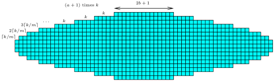
Figure 1: $S^{k}_{m}(a,b)$ with $m=5$, $k=5$, $a=2$ and $b=7$.

Observe that, since $k\geq m$, $\lceil k/m\rceil\leq 2k/m$, and therefore

$$x_{0}=b+(a+1)k+\sum_{i=1}^{m-1}i\lceil k/m\rceil=b+(a+1)k+\lceil k/m\rceil\frac{m(m-1)}{2}\leq b+(m+a)k,$$

so

$$S^{k}_{m}(a,b)\subseteq[-b-(m+a)k,b+(m+a)k]\times[-m-a-1,m+a+1].$$ (5)

In particular,

$$S^{k}_{m}(0,0)\subseteq[-2mk,2mk]\times[-2m,2m]\qquad\text{and}\qquad|S^{k}_{m}(0,0)|\leq 25m^{2}k.$$ (6)

Moreover, since $x_{i}\geq x_{i+1}+1$ for $m\leq i\leq m+a$ (i.e. the length of each row increases by at least one unit to the left and to the right) and a symmetric observation for rows $-m\leq i\leq-m-a$, we get

$$S^{k}_{m}(2a,0)\supseteq[-a,a]\times[-a,a].$$ (7)

A set of vertices $U\subseteq[n]^{2}$ is said to be active if all its vertices are active. Note that $S^{k}_{m}(a,b)\subseteq S^{k}_{m}(a+1,b)$. The next lemma shows that, if $S^{k}_{m}(a,b)$ is active and all vertices in $S^{k}_{m}(a+1,b)$ are good (or already active), then eventually $S^{k}_{m}(a+1,b)$ becomes active too.

Lemma 7.

Given any integers $a,b\geq 0$, $1\leq m<k$ and $r\leq\lceil k/m\rceil$, suppose that $S^{k}_{m}(a,b)$ is active and all vertices in $S^{k}_{m}(a+1,b)$ are $m$-good or active in the $r$-majority bootstrap percolation process. Then, deterministically $S^{k}_{m}(a+1,b)$ eventually becomes active.

Proof.

Put $k^{\prime}=\lceil k/m\rceil\geq 2$. Note that any vertex with at least $2k+k^{\prime}$ active neighbours has at most $2k+2-k^{\prime}$ inactive neighbours, and thus becomes active since $(2k+k^{\prime})-(2k+2-k^{\prime})=2(k^{\prime}-1)\geq k^{\prime}\geq r$. Our first goal is to show that we can make active one extra vertex to the right and to the left of each row in $S^{k}_{m}(a,b)$. Let $x_{i}$ be as in (4). For each $0\leq i\leq m+a+1$, consider the vertex $v_{i}=(x_{i}+1,i)$. Observe that $v_{i}\in S^{k}_{m}(a+1,b)$, so it must be active or good. If $v_{i}$ is active, then we are already done. Suppose otherwise that $v_{i}$ is good. By the definition of $S^{k}_{m}(a,b)$, $v_{i}$ has at least $\min\{k+(i-1)k^{\prime},2k\}$ neighbours in $S^{k}_{m}(a,b)$ one row below, and $\max\{k-ik^{\prime},0\}$ one row above, so in particular at least $2k-k^{\prime}$ neighbours in $S^{k}_{m}(a,b)$, which are active. Additionally, since $v_{i}$ is good, it has at least $2k^{\prime}$ extra active neighbours above and to the right, so it becomes active. By symmetry, we conclude that, for every $|i|\leq m+a+1$, vertices $(-x_{i}-1,i)$ and $(x_{i}+1,i)$ become active. Therefore, all vertices in $S^{k}_{m}(a,b+1)$ become active.

A close inspection of (4) yields the following chain of inclusions:

$$S^{k}_{m}(a,b)\subseteq S^{k}_{m}(a,b+1)\subseteq\cdots S^{k}_{m}(a,b+k)\subseteq S^{k}_{m}(a+1,b).$$ (8)

In view of this, the same argument can be inductively applied to show that for every $0\leq j\leq k-1$, if all vertices in $S^{k}_{m}(a,b+j)$ are active, then we eventually reach a state in which all vertices in $S^{k}_{m}(a,b+j+1)$ become active as well. (Note that the argument requires that the newly added vertices $v_{i}$ satisfy $v_{i}\in S^{k}_{m}(a+1,b)$, which follows from (8).)

Finally, observe that all vertices in $[-b,b]\times\{-m-a-2,m+a+2\}$ have $2k+1$ neighbours in $S^{k}_{m}(a,b+k)$ (either in the row below or the row above). Since these vertices are good, they have at least $4k^{\prime}$ active neighbours not in $S^{k}_{m}(a,b+k)$, and thus they become active too. We showed that all vertices in $S^{k}_{m}(a+1,b)$ became active, and the proof of the lemma is finished. ∎

We consider two other graphs $\mathscr{L}_{1}(n)$ and $\mathscr{L}_{\infty}(n)$ on the same vertex set $[n]^{2}$ as $\mathscr{L}(n,k)$. Two vertices $(x,y)$ and $(x^{\prime},y^{\prime})$ in $[n]^{2}$ are adjacent in $\mathscr{L}_{1}(n)$ if

$$\begin{cases}x^{\prime}=x\\ y^{\prime}-y\equiv\pm 1\mod n;\end{cases}\qquad\text{or}\qquad\begin{cases}y^{\prime}=y\\ x^{\prime}-x\equiv\pm 1\mod n.\end{cases}$$

Similarly, $(x,y)$ and $(x^{\prime},y^{\prime})$ are adjacent in $\mathscr{L}_{\infty}(n)$ if

$$(x,y)\neq(x^{\prime},y^{\prime})\qquad\text{and}\qquad\begin{cases}x^{\prime}-x\equiv 0,\pm 1\mod n\\ y^{\prime}-y\equiv 0,\pm 1\mod n.\end{cases}$$

In other words, $\mathscr{L}_{1}(n)$ is the classical square lattice $n\times n$, and $\mathscr{L}_{\infty}(n)$ is the same lattice with diagonals added. Given any two vertices $u,v\in[n]^{2}$, the $\ell_{1}$-distance and $\ell_{\infty}$-distance between $u$ and $v$ respectively denote their graph distance in $\mathscr{L}_{1}(n)$ and $\mathscr{L}_{\infty}(n)$. (These correspond to the usual $\ell_{1}$- and $\ell_{\infty}$-distances on the torus.) Also, we say that a set $U\subseteq[n]^{2}$ is $\ell_{1}$-connected (or $\ell_{\infty}$-connected) if the subgraph of $\mathscr{L}_{1}(n)$ (or $\mathscr{L}_{\infty}(n)$) induced by $U$ is a connected graph. Given two sets $U,U^{\prime}\subseteq[n]^{2}$, we say $U^{\prime}$ is a translate of $U$ if there exists $(x,y)\in\mathbb{Z}^{2}$ such that $U^{\prime}=(x,y)+U$ (recall that we interpret coordinates modulo $n$).

Lemma 8.

Let $k,m,r\in\mathbb{Z}$ satisfying $1\leq m<k$ and $r\leq\lceil k/m\rceil$. Suppose that $U\subseteq[n]^{2}$ has the following properties: $U$ is $\ell_{1}$-connected; all vertices in $[n]^{2}$ within $\ell_{1}$-distance at most $32mk^{2}$ from $U$ are $m$-good (or active); and $U$ contains an active set $S$ which is a translate of $S^{k}_{m}(0,0)$. Then, eventually $U$ becomes active in the $r$-majority bootstrap percolation process.

Proof.

Without loss of generality, we assume that $S=S^{k}_{m}(0,0)$ (by changing the coordinates appropriately). Then, by (6), $S$ is contained inside the square $Q=[-2mk,2mk]\times[-2mk,2mk]$. We weaken our hypothesis that $S\subseteq U$, and only assume that $Q\cap U\neq\emptyset$. Let $S^{\prime}=S^{k}_{m}(14mk,0)$. By (5), $S^{\prime}\subseteq[-15mk^{2},15mk^{2}]\times[-15mk^{2},15mk^{2}]$. Therefore, every vertex in $S^{\prime}$ must lie within $\ell_{1}$-distance $30mk^{2}+4mk\leq 32mk^{2}$ from $U$, and thus must be good (or already active). We repeatedly apply Lemma 7 and conclude that $S^{\prime}$ eventually becomes active. By (7), $S^{k}_{m}(14mk,0)\supseteq[-7mk,7mk]^{2}$, so $S^{\prime}$ contains not only the square $Q$, but all $8$ translated copies of $Q$ around it. More precisely, for every $i,j\in\{-1,0,1\}$,

$$S^{\prime}\supseteq Q_{ij},\qquad\text{where}\qquad Q_{ij}=(4mk+1)(i,j)+Q.$$

Hence, all nine squares $Q_{ij}$ eventually become active.

Note that, for any $x,y\in\mathbb{Z}$, the translate $\hat{Q}=(x,y)+Q$ contains $\hat{S}=(x,y)+S$. Therefore, if $\hat{Q}$ is active and intersects $U$, the argument above shows that all nine squares

$$\hat{Q}_{ij}=(4mk+1)(i,j)+\hat{Q}$$

eventually become active as well. We may iteratively repeat the same argument to any active translate of $Q$ that intersects $U$. Since $U$ is $\ell_{1}$-connected, we can find a collection of translates of $Q$ that eventually become active and whose union contains $U$. This finishes the proof of the lemma. ∎

2.1 The $t$-tessellation

Given any integer $1\leq t\leq n$, we define the $t$-tessellation $\mathcal{T}(n,t)$ of $[n^{2}]$ to be the partition of $[n]^{2}$ into cells

$$C_{ij}=[a_{i}+1,a_{i+1}]\times[a_{j}+1,a_{j+1}],\qquad 0\leq i,j\leq\lfloor n/t\rfloor-1,$$

where $a_{i}=it$ for $0\leq i\leq\lfloor n/t\rfloor-1$ and $a_{\lfloor n/t\rfloor}=n$. Most cells in $\mathcal{T}(n,t)$ are squares with $t$ vertices on each side, except for possibly those cells on the last row or column if $t\nmid n$. These exceptional cells are in general rectangles, and have between $t$ and $2t$ vertices on each side.

We may regard the set of cells $\mathcal{T}(n,t)$ of the $t$-tessellation as the vertex set of either $\mathscr{L}_{1}(\lfloor n/t\rfloor)$ or $\mathscr{L}_{\infty}(\lfloor n/t\rfloor)$ (that is, $\mathcal{T}(n,t)\simeq\big{[}\lfloor n/t\rfloor\big{]}^{2}$) by identifying each cell $C_{ij}\in\mathcal{T}(n,t)$ with $(i,j)\in\big{[}\lfloor n/t\rfloor\big{]}^{2}$. Call each of the resulting graphs $\mathscr{L}_{1}(n,t)$ and $\mathscr{L}_{\infty}(n,t)$, respectively. In other words, the vertices of $\mathscr{L}_{1}(n,t)$ are precisely the cells in $\mathcal{T}(n,t)\simeq\big{[}\lfloor n/t\rfloor\big{]}^{2}$, and each cell is adjacent to its neighbouring cells at the top, bottom, left and right (in a toroidal sense); and a similar description (adding the top-right, top-left, bottom-right and bottom-left cells to the neighbourhood) holds for $\mathscr{L}_{\infty}(n,t)$. To avoid confusion, we always call the vertices of $\mathscr{L}_{1}(n,t)\simeq\mathscr{L}_{1}(\lfloor n/t\rfloor)$ and $\mathscr{L}_{\infty}(n,t)\simeq\mathscr{L}_{\infty}(\lfloor n/t\rfloor)$ cells, and reserve the word vertex for the original graph $\mathscr{L}(n,k)$.

For $i\in\{1,\infty\}$, we say that a set of cells $\mathcal{Z}\subseteq\mathcal{T}(n,t)$ is $\ell_{i}$-connected, if $\mathcal{Z}$ induces a connected subgraph of $\mathscr{L}_{i}(n,t)$. Also, the $\ell_{i}$-distance between two cells $C$ and $C^{\prime}$ corresponds to their graph distance in the graph of cells $\mathscr{L}_{i}(n,t)$. This should not be confused with the $\ell_{i}$-distance (in $\mathscr{L}_{i}(n)$) between the vertices inside $C$ and $C^{\prime}$. Sometimes, we will also refer to the $\ell_{i}$-distance between a vertex $v$ and a cell $C$. By this, we mean the minimum distance in $\mathscr{L}_{i}(n)$ between $v$ and any vertex $u\in C$.

Given $1\leq m\leq k$, we say that a cell $C\in\mathcal{T}(n,t)$ is $m$-good (or simply good) if every vertex inside or within $\ell_{1}$-distance $32mk^{2}$ of $C$ is good or active. Otherwise, we call it bad. Note that deciding whether a cell $C$ is good or bad only depends on the status of the vertices inside or within $\ell_{1}$-distance $32mk^{2}+k+1$ from $C$. We call a cell a seed if it contains an active translate of $S^{k}_{m}(0,0)$. (By (6), this definition is not vacuous if $t\geq 4mk+1$.)

In view of all these definitions, Lemma 8 directly implies the following corollary.

Corollary 9.

Let $k,m,r,t\in\mathbb{Z}$ satisfying $1\leq m<k$, $r\leq\lceil k/m\rceil$ and $1\leq t\leq n$. Suppose that $\mathcal{Z}$ is an $\ell_{1}$-connected set of cells in $\mathcal{T}(n,t)$ such that all cells in $\mathcal{Z}$ are $m$-good and $\mathcal{Z}$ contains a seed. Then, in the $r$-majority bootstrap percolation process, eventually all cells in $\mathcal{Z}$ become active.

3 Percolative ingredients

In this section, we consider the $t$-tessellation $\mathcal{T}(n,t)$ defined in Section 2.1 for an appropriate choice of $t$. We combine the deterministic results in Section 2 together with some percolation techniques to conclude that eventually most cells in $\mathcal{T}(n,t)$ (and thus most vertices in $\mathscr{L}(n,k)$) will eventually become active a.a.s. This corresponds to Phase 1 described in the introduction.

Throughout the section, we define $\widetilde{n}=\lfloor n/t\rfloor$ and assume that $\widetilde{n}\to\infty$ as $n\to\infty$. We identify the set of cells $\mathcal{T}(n,t)$ with $[\widetilde{n}]^{2}$ in the terms described in Section 2.1, and consider the graphs of cells $\mathscr{L}_{1}(n,t)\simeq\mathscr{L}_{1}(\widetilde{n})$ and $\mathscr{L}_{\infty}(n,t)\simeq\mathscr{L}_{\infty}(\widetilde{n})$. Recall (for $i\in\{1,\infty\}$) the definitions of $\ell_{i}$-connected sets of cells and $\ell_{i}$-distance between cells from that section. Moreover, define an $\ell_{i}$-path of cells to be a path in the graph $\mathscr{L}_{i}(\widetilde{n})$, and the $\ell_{i}$-diameter of an $\ell_{i}$-connected set of cells $\mathcal{Z}$ to be the maximal $\ell_{i}$-distance between two cells $C,C^{\prime}\in\mathcal{Z}$. (The $\ell_{i}$-diameter of $\mathcal{Z}$ is also denoted $\operatorname{diam}_{\ell_{i}}\mathcal{Z}$.) Finally, given a set of cells $\mathcal{Z}$, an $\ell_{i}$-component of $\mathcal{Z}$ is a subset $\mathcal{C}\subseteq\mathcal{Z}$ that induces a connected component of the subgraph of $\mathscr{L}_{i}(\widetilde{n})$ induced by $\mathcal{Z}$.

We need one more definition to characterize very large sets of cells that “spread almost everywhere” in $[\widetilde{n}]^{2}$. Set $A=10^{8}$ hereafter. Given any $\varepsilon=\varepsilon(\widetilde{n})\in(0,1)$ and a set of cells $\mathcal{Z}\subseteq[\widetilde{n}]^{2}$, we say that $\mathcal{Z}$ is $\varepsilon$-ubiquitous if it satisfies the following properties:

• $\mathcal{Z}$ is an $\ell_{1}$-connected set of cells;

• $|\mathcal{Z}|\geq(1-A\varepsilon)\widetilde{n}^{2}$; and

• given any collection $\mathcal{B}_{1},\mathcal{B}_{2},\ldots,\mathcal{B}_{j}$ of disjoint $\ell_{\infty}$-connected non-empty subsets of $[\widetilde{n}]^{2}\setminus\mathcal{Z}$,

  $$\min_{1\leq i\leq j}\big{\{}\operatorname{diam}_{\ell_{\infty}}\mathcal{B}_{i}\big{\}}\leq\frac{A}{\log(1/\varepsilon)}\log\left(\widetilde{n}^{2}/j\right).$$ (9)

In particular, (iii) implies that

• every $\ell_{\infty}$-connected set of cells $\mathcal{B}\subseteq[\widetilde{n}]^{2}\setminus\mathcal{Z}$ has $\ell_{\infty}$-diameter at most $\frac{A}{\log(1/\varepsilon)}\log(\widetilde{n}^{2})$.

Our goal for this section is to show that a.a.s. there is an $\varepsilon$-ubiquitous set of cells that eventually become active. As a first step towards this, we adapt some ideas from percolation theory to find an $\varepsilon$-ubiquitous set of good cells in $[\widetilde{n}]^{2}$. We formulate this in terms of a slightly more general context. A $2$-dependent site-percolation model on $\mathscr{L}_{1}(\widetilde{n})$ is any probability space defined by the state (good or bad) of the cells in $[\widetilde{n}]^{2}$ such that the state of each cell $C$ is independent from the state of all other cells at $\ell_{1}$-distance at least $3$ from $C$. We represent such probability space by means of the random vector $\text{\boldmath$X$}=(X_{C})_{C\in[\widetilde{n}]^{2}}$, where $X_{C}$ is the indicator function of the event that a cell $C$ is good. In this setting, let $\mathcal{G}=\{C\in[\widetilde{n}]^{2}:X_{C}=1\}$ be the set of all good cells, and let $\mathcal{G}_{0}$ be the largest $\ell_{1}$-component of $\mathcal{G}$ (if $\mathcal{G}$ has more than one $\ell_{1}$-component of maximal size, pick one by any fixed deterministic rule).

Lemma 10.

Let $\epsilon_{0}>0$ be a sufficiently small constant. Given any $\epsilon=\epsilon(\widetilde{n})$ satisfying $\widetilde{n}^{-1/3}<\epsilon\leq\epsilon_{0}$, consider a $2$-dependent site-percolation model $X$ on $\mathscr{L}_{1}(\widetilde{n})$, where each cell in $[\widetilde{n}]^{2}$ is good with probability at least $1-\epsilon$. Then, a.a.s. as $\widetilde{n}\to\infty$, the largest $\ell_{1}$-component $\mathcal{G}_{0}$ of the set of good cells is $\epsilon$-ubiquitous.

Proof.

Throughout the argument, we assume that $\epsilon_{0}$ is sufficiently small so that $\epsilon$ meets all the conditions required. Let $\overline{\mathcal{G}}_{0}=[\widetilde{n}]^{2}\setminus\mathcal{G}_{0}$. Our first goal is to show the following claim.

Claim 1.

A.a.s. every $\ell_{\infty}$-component of $\overline{\mathcal{G}}_{0}$ has $\ell_{\infty}$-diameter at most $\widetilde{n}/2$.

For this purpose, we will use a classical result by Liggett, Schonmann, and Stacey (cf. Theorem 0.0 in [16]) that compares $X$ with the product measure. Given a constant $0<p_{0}<1$ (sufficiently close to $1$), consider $\widehat{\text{\boldmath$X$}}=(\widehat{X}_{C})_{C\in[\widetilde{n}]^{2}}$, in which the $\widehat{X}_{C}$ are independent indicator variables satisfying ${\bf Pr}(\widehat{X}_{C}=1)=p_{0}$, and define $\widehat{\mathcal{G}}=\{C\in[\widetilde{n}]^{2}:\widehat{X}_{C}=1\}$. If $\epsilon_{0}$ (and thus $\epsilon$) is small enough given $p_{0}$, then our 2-dependent site-percolation model $X$ stochastically dominates $\widehat{\text{\boldmath$X$}}$, that is, ${\bf E}(F(\mathcal{G}))\geq{\bf E}(F(\widehat{\mathcal{G}}))$ for every non-decreasing function $F$ over the power set $2^{[\widetilde{n}]^{2}}$ (i.e. satisfying $F(\mathcal{Z})\leq F(\mathcal{Z}^{\prime})$ for every $\mathcal{Z}\subseteq\mathcal{Z}^{\prime}\subseteq[\widetilde{n}]^{2}$).

Set $s=\lfloor\widetilde{n}/4\rfloor$ and, for $i,j\in\{0,1,2,3,4\}$, consider the rectangles (in $\mathbb{Z}^{2}$)

$$\mathcal{R}_{i,j}=(is,js)+[1,s]\times[1,2s]\quad\text{and}\quad\mathcal{R}^{\prime}_{i,j}=(is,js)+[1,2s]\times[1,s].$$

We regard $\mathcal{R}_{i,j}$ and $\mathcal{R}^{\prime}_{i,j}$ as subsets of the torus $[\widetilde{n}]^{2}$ by interpreting their coordinates modulo $n$. Note that, if $4\mid\widetilde{n}$ then some of these rectangles are repeated (e.g. $\mathcal{R}_{0,0}=\mathcal{R}_{4,0}$), but this does not pose any problem for our argument. Let $\mathcal{R}$ be any of the rectangles above and $\mathcal{Z}\subseteq[\widetilde{n}]^{2}$ be any set of cells. We say that $\mathcal{Z}$ is $\ell_{1}$-crossing for $\mathcal{R}$ if the set $\mathcal{Z}\cap\mathcal{R}$ has some $\ell_{1}$-component intersecting the four sides of $\mathcal{R}$. It is easy to verify that if $\mathcal{Z}$ is $\ell_{1}$-crossing for all $\mathcal{R}_{i,j}$ and all $\mathcal{R}^{\prime}_{i,j}$, then every $\ell_{\infty}$-component of $[\widetilde{n}]^{2}\setminus\mathcal{Z}$ has $\ell_{\infty}$-diameter at most $2s\leq\widetilde{n}/2$. If $p_{0}$ is sufficiently close to $1$, by applying a result by Deuschel and Pisztora (cf. Theorem 1.1 in [10]) to all $\mathcal{R}_{i,j}$ and all $\mathcal{R}^{\prime}_{i,j}$, we conclude that a.a.s. $\widehat{\mathcal{G}}$ contains an $\ell_{1}$-component with more than $\widetilde{n}^{2}/2$ cells which is $\ell_{1}$-crossing for all $\mathcal{R}_{i,j}$ and all $\mathcal{R}^{\prime}_{i,j}$. This is a non-decreasing event, and hence a.a.s. $\mathcal{G}$ has an $\ell_{1}$-component with exactly the same properties (which must be $\mathcal{G}_{0}$ by its size). This implies the claim.

In view of Claim 1, we will restrict our focus to $\ell_{\infty}$-components of $\overline{\mathcal{G}}_{0}$ of small $\ell_{\infty}$-diameter. Let $N_{d}$ be the number of cells that belong to $\ell_{\infty}$-components of $\overline{\mathcal{G}}_{0}$ of $\ell_{\infty}$-diameter $d$. Then, the following holds.

Claim 2.

For every $0\leq d\leq\widetilde{n}/2$,

$${\bf E}N_{d}\leq B\widetilde{n}^{2}\epsilon^{\lceil(d+1)/4\rceil}\quad(B=10^{6})\qquad\text{and}\qquad{\bf Var}N_{d}\leq(4d+5)^{2}{\bf E}N_{d}.$$

In order to prove this claim, we need one definition. A special sequence of length $j$ is a sequence of $j+1$ different cells $C_{0},C_{1},\ldots,C_{j}$ in $[\widetilde{n}]^{2}$ such that any two consecutive cells in the sequence are at $\ell_{\infty}$-distance exactly $3$, and any two different cells are at $\ell_{\infty}$-distance at least $3$. Observe that there are at most $24^{j}$ special sequences of length $j$ starting at a given cell $C_{0}$. Moreover, by construction, the states (good or bad) of the cells in a special sequence are mutually independent.

We now proceed to the proof of Claim 2. Let $\mathcal{B}$ be an $\ell_{\infty}$-component of $\overline{\mathcal{G}}_{0}$ of $\ell_{\infty}$-diameter $0\leq d\leq\widetilde{n}/2$, and let $\mathcal{F}$ be the set of cells inside $\mathcal{B}$ but at $\ell_{1}$-distance $1$ of some cell in $\mathcal{G}_{0}$. $\mathcal{F}$ is $\ell_{\infty}$-connected (since $\mathscr{L}_{1}(\widetilde{n})$ and $\mathscr{L}_{\infty}(\widetilde{n})$ are dual lattices) and only contains bad cells. Moreover, $\mathcal{F}$ must contain two cells $C$ and $C^{\prime}$ at $\ell_{\infty}$-distance $d$ (with $C=C^{\prime}$ if and only if $d=0$). Let $P=C_{1},C_{2},\ldots,C_{m}$ be a path joining $C=C_{0}$ and $C^{\prime}=C_{m}$ in the subgraph of $\mathscr{L}_{\infty}(\widetilde{n})$ induced by $\mathcal{F}$. From this path, we construct a special sequence $Q=D_{0},D_{1},\ldots,D_{\lfloor d/3\rfloor}$ as follows. Set $D_{0}=C_{0}$ and, for $1\leq i\leq\lfloor d/3\rfloor$, $D_{i}=C_{j+1}$, where $C_{j}$ is the last cell in $P$ at $\ell_{\infty}$-distance at most $2$ from $D_{i-1}$. By construction, $Q$ is a special sequence of length $\lfloor d/3\rfloor$ contained in $\mathcal{B}$ and it consists of only bad cells. Therefore, if any given cell $D\in[\widetilde{n}]^{2}$ belongs to an $\ell_{\infty}$-component of $\overline{\mathcal{G}}_{0}$ of $\ell_{\infty}$-diameter $d$, then there must be a special sequence of bad cells and length $\lfloor d/3\rfloor$ starting within $\ell_{\infty}$-distance $d$ from $D$. This happens with probability at most

$$(2d+1)^{2}24^{\lfloor d/3\rfloor}\epsilon^{1+\lfloor d/3\rfloor}\leq B\epsilon^{\lceil(d+1)/4\rceil},$$

where it is straightforward to verify that the last inequality holds for $B=10^{6}$ and all $d$, as long as $\epsilon_{0}$ is sufficiently small. Summing over all $\widetilde{n}^{2}$ cells, we get the desired upper bound on ${\bf E}N_{d}$. To bound the variance, we consider separately pairs of cells that are within $\ell_{\infty}$-distance greater than $2d+2$ and at most $2d+2$, and we get

$${\bf E}({N_{d}}^{2})\leq({\bf E}N_{d})^{2}+(4d+5)^{2}{\bf E}N_{d},$$

so

$${\bf Var}N_{d}\leq(4d+5)^{2}{\bf E}N_{d}.$$

This proves Claim 2. Next, let $N^{\prime}_{d}=\sum_{i\geq d}N_{i}$ be the number of cells that belong to $\ell_{\infty}$-components of $\overline{\mathcal{G}}_{0}$ of $\ell_{\infty}$-diameter at least $d$. Then, we have the next claim.

Claim 3.

A.a.s. for every $d\geq 0$, $N^{\prime}_{d}<B^{\prime}\widetilde{n}^{2}\epsilon^{\lceil(d+1)/5\rceil}$, where $B^{\prime}=11B$.

Suppose first that ${\bf E}N_{d}\geq\widetilde{n}^{1/2}$. By Claim 2, we must have $(1/\epsilon)^{\lceil(d+1)/4\rceil}\leq B\widetilde{n}^{3/2}$, so in particular $d\leq\log\widetilde{n}$. Then, using Chebyshev’s inequality and the bounds in Claim 2,

$${\bf Pr}\left(N_{d}\geq 2{\bf E}N_{d}\right)\leq\frac{{\bf Var}N_{d}}{({\bf E}N_{d})^{2}}\leq\frac{(4d+5)^{2}}{{\bf E}N_{d}}\leq\frac{25\log^{2}\widetilde{n}}{\widetilde{n}^{1/2}}.$$ (10)

Summing the probabilities over all $0\leq d\leq\log\widetilde{n}$, the probability is still $o(1)$. Suppose otherwise that ${\bf E}N_{d}\leq\widetilde{n}^{1/2}$. By Markov’s inequality,

$${\bf Pr}\left(N_{d}\geq\widetilde{n}^{2}\epsilon^{\lceil(d+1)/5\rceil}\right)\leq\frac{{\bf E}N_{d}}{\widetilde{n}^{2}\epsilon^{\lceil(d+1)/5\rceil}}.$$ (11)

Recall from Claim 2 and our assumptions that ${\bf E}N_{d}\leq\min\left\{\widetilde{n}^{1/2},B\widetilde{n}^{2}\epsilon^{\lceil(d+1)/4\rceil}\right\}$. If $\widetilde{n}^{1/2}\leq B\widetilde{n}^{2}\epsilon^{\lceil(d+1)/4\rceil}$, then (11) becomes

$${\bf Pr}\left(N_{d}\geq\widetilde{n}^{2}\epsilon^{\lceil(d+1)/5\rceil}\right)\leq\frac{1}{\widetilde{n}^{3/2}\epsilon^{\lceil(d+1)/5\rceil}}.$$

For $0\leq d\leq 15$, the bound above is $o(1)$ as long as say $\epsilon\geq\widetilde{n}^{-1/3}$. For $d\geq 16$, we have $\lceil(d+1)/5\rceil+(d+1)/100\leq 0.95\lceil(d+1)/4\rceil$, and therefore

$${\bf Pr}\left(N_{d}\geq\widetilde{n}^{2}\epsilon^{\lceil(d+1)/5\rceil}\right)\leq\frac{1}{\widetilde{n}^{3/2}\epsilon^{\lceil(d+1)/5\rceil}}\leq\frac{\epsilon^{(d+1)/100}}{\widetilde{n}^{3/2}\epsilon^{0.95\lceil(d+1)/4\rceil}}\leq\frac{B^{0.95}\epsilon^{(d+1)/100}}{\widetilde{n}^{0.075}},$$

where for the last step we used that $(1/\epsilon)^{\lceil(d+1)/4\rceil}\leq B\widetilde{n}^{3/2}$. Summing the bound above over all $d\geq 16$ gives again a contribution of $o(1)$. Finally, if $B\widetilde{n}^{2}\epsilon^{\lceil(d+1)/4\rceil}\leq\widetilde{n}^{1/2}$, then we must have $d\geq 16$ since $\epsilon\geq\widetilde{n}^{-1/3}$. Therefore (11) becomes

$${\bf Pr}\left(N_{d}\geq\widetilde{n}^{2}\epsilon^{\lceil(d+1)/5\rceil}\right)\leq\frac{B\widetilde{n}^{2}\epsilon^{\lceil(d+1)/4\rceil}}{\widetilde{n}^{2}\epsilon^{\lceil(d+1)/5\rceil}}\leq B\epsilon^{0.05\lceil(d+1)/4\rceil+(d+1)/100}\leq\frac{B^{0.95}\epsilon^{(d+1)/100}}{\widetilde{n}^{0.075}},$$

where for the last step we used that $\epsilon^{\lceil(d+1)/4\rceil}\leq\widetilde{n}^{-3/2}/B$. Summing the bound above over all $d\geq 16$ gives $o(1)$. Putting all the previous cases together, we conclude that a.a.s. for all $0\leq d\leq\widetilde{n}/2$,

$$N_{d}\leq\max\left\{\widetilde{n}^{2}\epsilon^{\lceil(d+1)/5\rceil},2{\bf E}N_{d}\right\}\leq 2B\widetilde{n}^{2}\epsilon^{\lceil(d+1)/5\rceil}.$$

The same is true for $d\geq\widetilde{n}/2$ by Claim 1. Hence, a.a.s. for all $d\geq 0$,

$$N^{\prime}_{d}=\sum_{i\geq d}N_{i}\leq 2B\widetilde{n}^{2}\epsilon^{\lceil(d+1)/5\rceil}\sum_{i\geq 0}5\epsilon^{i}<11B\widetilde{n}^{2}\epsilon^{\lceil(d+1)/5\rceil}.$$

This proves Claim 3.

Finally, assume that the a.a.s. event in Claim 3 holds. Given any $1\leq j\leq\widetilde{n}^{2}$, set

$$d=\left\lfloor\frac{5\log(B^{\prime}\widetilde{n}^{2}/j)}{\log(1/\epsilon)}\right\rfloor.$$

Then, $\lceil(d+1)/5\rceil\geq\frac{\log(B^{\prime}\widetilde{n}^{2}/j)}{\log(1/\epsilon)}$, and so

$$N^{\prime}_{d}<B^{\prime}\widetilde{n}^{2}\epsilon^{\lceil(d+1)/5\rceil}\leq j.$$

Therefore, given any disjoint $\ell_{\infty}$-connected non-empty sets $\mathcal{B}_{1},\mathcal{B}_{2},\ldots,\mathcal{B}_{j}\subseteq\overline{\mathcal{G}}_{0}$ (not necessarily components), at least one of the $j$ sets must have $\ell_{\infty}$-diameter strictly less than $d$. Hence,

$$\min_{1\leq i\leq j}\big{\{}\operatorname{diam}_{\ell_{\infty}}\mathcal{B}_{i}\big{\}}\leq d-1\leq\frac{5\log(\widetilde{n}^{2}/j)+5\log B^{\prime}}{\log(1/\epsilon)}-1\leq\frac{5\log(\widetilde{n}^{2}/j)}{\log(1/\epsilon)}.$$

This proves part (iii) of the definition of $\epsilon$-ubiquitous for $\mathcal{G}_{0}$. Part (i) is immediate since $\mathcal{G}_{0}$ is $\ell_{1}$-connected by definition. Finally, since $N^{\prime}_{0}<B^{\prime}\widetilde{n}^{2}\epsilon$, then $|\mathcal{G}_{0}|>\widetilde{n}^{2}(1-B^{\prime}\epsilon)$, which implies part (ii). So $\mathcal{G}_{0}$ is $\epsilon$-ubiquitous. ∎

The next result combines Corollary 9 and Lemma 10 in order to show that most of the cells become active during Phase 1 of the process.

Proposition 11.

Let $0<p_{0}<1$ be a sufficiently small constant. Given any $p=p(n)\in\mathbb{R}$, $k=k(n)\in\mathbb{N}$ and $r=r(n)\in\mathbb{Z}$ satisfying (eventually for all $n\in\mathbb{N}$ sufficiently large)

$$200\frac{(\log\log n)^{2/3}}{\log^{1/3}n}\leq p\leq p_{0},\qquad\frac{1000}{p}\log(1/p)\leq k\leq\frac{p^{2}\log n}{3000\log(1/p)},\qquad\text{and}\qquad r\leq pk/9,$$ (12)

define

$$t=t(n)=100k^{3}\qquad\text{and}\qquad\varepsilon=\varepsilon(n)=k^{-100}.$$ (13)

Consider the $r$-majority bootstrap percolation process $\mathbb{M}_{r}(\mathscr{L}(n,k);p)$, and the $t$-tessellation $\mathcal{T}(n,t)$ of $[n]^{2}$ into $\widetilde{n}^{2}=\lfloor n/t\rfloor^{2}$ cells. Then, a.a.s. the set of all cells that eventually become active contains an $\varepsilon$-ubiquitous $\ell_{1}$-component.

Proof.

Assume that $p_{0}$ is sufficiently small and $n$ sufficiently large so that the parameters $p$, $k$, $t$ and $\varepsilon$ satisfy all the required conditions below in the argument. (In particular, we may assume that $k,r,t$ are larger than a sufficently large constant, and $\varepsilon$ is smaller than a sufficiently small constant.) Define $k_{0}=\left\lceil\frac{1000}{p}\log(1/p)\right\rceil$ and $k_{1}=\left\lfloor\frac{p^{2}\log n}{3000\log(1/p)}\right\rfloor$. From (12) and since $p_{0}$ is small enough,

$$k_{0}<\frac{2000}{p}\log(1/p)=\frac{2000p^{2}\log^{2}(1/p)}{p^{3}\log(1/p)}\leq\frac{2000}{200^{3}}\frac{p^{2}\log n}{\log(1/p)}<k_{1},$$ (14)

so there exist $k\in\mathbb{N}$ satisfying $k_{0}\leq k\leq k_{1}$, and thus the statement is not vacuous. Later in the argument we will need the bound

$$\frac{pk}{8}=\frac{pk}{8\log k}\log k\geq\frac{pk_{0}}{8\log k_{0}}\log k\geq\frac{900}{8}\log k\geq 111\log k.$$ (15)

Define $m=\lceil 8/p\rceil$, so in particular

$$m<\frac{9}{p}<k_{0}\leq k,$$

as required for the definition of $m$-good. Moreover, $k\leq k_{1}<\log n<\frac{n-1}{2}$, so every vertex of $\mathscr{L}(n,k)$ has exactly $4k+2$ neighbours (i.e. neighbourhoods in $\mathscr{L}(n,k)$ do not wrap around the torus). The number of vertices that are initially active in a set of $k$ vertices is distributed as the random variable $\operatorname{Bin}(k,p)$. Thus, by Chernoff bound (see, e.g., Theorem 4.5(2) in [17]), the probability that a vertex is initially $m$-bad is at most

$$4{\bf Pr}\big{(}\operatorname{Bin}(k,p)<2\lceil k/m\rceil\big{)}\leq 4{\bf Pr}\big{(}\operatorname{Bin}(k,p)\leq(1-1/2)pk\big{)}\leq 4\exp(-pk/8),$$ (16)

where we used that $2\lceil k/m\rceil\leq 2\lceil pk/8\rceil\leq pk/2$.

Now consider the $t$-tessellation $\mathcal{T}(n,t)$ of $[n]^{2}$ with $t=100k^{3}$. In particular, we have

$$t\leq 100{k_{1}}^{3}<\log^{3}n<n,$$ (17)

so $\mathcal{T}(n,t)$ is well defined. For each cell $C\in\mathcal{T}(n,t)$, let $X_{C}$ denote the indicator function of the event that $C$ is $m$-good. Recall that every cell $C$ is a rectangle with at most $2t$ vertices per side, and thus $C$ has at most $(2t+64mk^{2})^{2}\leq 300^{2}k^{6}$ vertices within $\ell_{1}$-distance $32mk^{2}$. Then, by (16), (15) and a union bound,

$${\bf Pr}(X_{C}=0)\leq 4(300^{2}k^{6})\exp(-pk/8)\leq 600^{2}k^{6}\exp(-111\log k)\leq(1/k)^{100}=\varepsilon.$$

Moreover, the outcome of $X_{C}$ is determined by the status (active or inactive) of all vertices within $\ell_{1}$-distance $32mk^{2}+k+1\leq 100mk^{2}\leq t$ from some vertex in $C$. All these vertices must belong to cells that are within $\ell_{1}$-distance at most $2$ from $C$ (recall that this refers to the distance in the graph of cells $\mathscr{L}_{1}(n,t)$). Therefore, for every cell $C\in\mathcal{T}(n,t)$ and set of cells $\mathcal{Z}\subseteq\mathcal{T}(n,t)$ such that $C$ is at $\ell_{1}$-distance greater than $2$ from all cells in $\mathcal{Z}$, the indicator $X_{C}$ is independent of $(X_{C^{\prime}})_{C^{\prime}\in\mathcal{Z}}$. Hence, $\text{\boldmath$X$}=(X_{C})_{C\in\mathcal{T}(n,t)}$ is a $2$-dependent site-percolation model on the lattice $\mathscr{L}_{1}(n,t)$ with ${\bf Pr}(X_{C}=1)\geq 1-\varepsilon$. Observe that $X$ satisfies the conditions of Lemma 10, assuming that $\varepsilon=(1/k)^{100}$ is small enough (which follows from our choice of $p_{0}$) and since $\varepsilon\geq{k_{1}}^{-100}>\log^{-100}n>\lfloor n/t\rfloor^{-1/3}$ (recall by (17) that $t\leq\log^{3}n$, so the number of cells in $\mathcal{T}(n,t)$ is $\widetilde{n}^{2}=\lfloor n/t\rfloor^{2}\to\infty$.) Then, by Lemma 10, the largest $\ell_{1}$-component $\mathcal{G}_{0}$ induced by the set of $m$-good cells is a.a.s. $\varepsilon$-ubiquitous. In particular

$${\bf Pr}\left(|\mathcal{G}_{0}|<(1-A\varepsilon)\lfloor n/t\rfloor^{2}\right)=o(1),$$ (18)

where $A=10^{8}$. We want to show that a.a.s. $\mathcal{G}_{0}$ contains a seed. For each cell $C\in\mathcal{T}(n,t)$, let $Y_{C}$ be the indicator function of the event that

$$S_{C}=(x+\lfloor t/2\rfloor,y+\lfloor t/2\rfloor)+S^{k}_{m}(0,0)$$

is initially active, where $(x,y)$ are the coordinates of the bottom left vertex in $C$. By (6), $S_{C}$ is contained in $C$, and at $\ell_{1}$-distance greater than $\lfloor t/2\rfloor-2mk>40k^{3}>32mk^{2}+k+1$ from any other cell in $\mathcal{T}(n,t)$, and therefore $Y_{C}$ depends only on vertices inside $C$ and at distance greater than $32mk^{2}+k+1$ from any other cell. In particular, $Y_{C}=1$ implies that $C$ is a seed. Moreover, for any two disjoint sets of cells $\mathcal{Z},\mathcal{Z}^{\prime}\subseteq\mathcal{T}(n,t)$, the random vectors $(Y_{C})_{C\in\mathcal{Z}}$ and $(X_{C^{\prime}})_{C^{\prime}\in\mathcal{Z}^{\prime}}$ are independent, since they are determined by the status of two disjoint sets of vertices. For the same reason, $(Y_{C})_{C\in\mathcal{Z}}$ and $(Y_{C^{\prime}})_{C^{\prime}\in\mathcal{Z}^{\prime}}$ are also independent. By (6) and (12), the probability that a cell $C$ is a seed is at least

$${\bf Pr}(Y_{C}=1)\geq p^{25m^{2}k}\geq p^{25(9/p)^{2}(p^{2}\log n)/(3000\log(1/p))}=e^{-(45^{2}/3000)\log n}\geq n^{-1}.$$ (19)

For each cell $C$, define $\bar{X}_{C}=1-X_{C}$ and $\bar{Y}_{C}=1-Y_{C}$. Moreover, for each set of cells $\mathcal{Z}$, let

$$X_{\mathcal{Z}}=\prod_{C\in\mathcal{Z}}X_{C},\qquad\bar{X}_{\mathcal{Z}}=\prod_{C\in\mathcal{Z}}\bar{X}_{C},\qquad Y_{\mathcal{Z}}=\prod_{C\in\mathcal{Z}}Y_{C}\qquad\text{and}\qquad\bar{Y}_{\mathcal{Z}}=\prod_{C\in\mathcal{Z}}\bar{Y}_{C}.$$

Now fix an $\ell_{1}$-connected set of cells $\mathcal{Z}$ containing at least an $1-A\varepsilon$ fraction of the cells, and let $\partial\mathcal{Z}$ be the set of cells not in $\mathcal{Z}$ but adjacent in $\mathscr{L}_{1}(n,t)$ to some cell in $\mathcal{Z}$ (i.e. the strict neighbourhood of $\mathcal{Z}$ in $\mathscr{L}_{1}(n,t)$). Since $A\varepsilon<1/2$, the event $\mathcal{G}_{0}=\mathcal{Z}$ is the same as $X_{\mathcal{Z}}\bar{X}_{\partial\mathcal{Z}}=1$. Furthermore,

$${\bf Pr}\big{(}(\bar{Y}_{\mathcal{Z}}=1)\cap(X_{\mathcal{Z}}\bar{X}_{\partial\mathcal{Z}}=1)\big{)} ={\bf Pr}\big{(}(\bar{Y}_{\mathcal{Z}}=1)\cap(\bar{X}_{\partial\mathcal{Z}}=1)\big{)}-{\bf Pr}\big{(}(\bar{Y}_{\mathcal{Z}}=1)\cap(X_{\mathcal{Z}}=0)\cap(\bar{X}_{\partial\mathcal{Z}}=1)\big{)}$$

$$\leq{\bf Pr}(\bar{Y}_{\mathcal{Z}}=1){\bf Pr}(\bar{X}_{\partial\mathcal{Z}}=1)-{\bf Pr}(\bar{Y}_{\mathcal{Z}}=1){\bf Pr}\big{(}(X_{\mathcal{Z}}=0)\cap(\bar{X}_{\partial\mathcal{Z}}=1)\big{)}$$

$$={\bf Pr}(\bar{Y}_{\mathcal{Z}}=1){\bf Pr}(X_{\mathcal{Z}}\bar{X}_{\partial\mathcal{Z}}=1),$$

where we used that $\bar{Y}_{\mathcal{Z}}$ and $\bar{X}_{\partial\mathcal{Z}}$ are independent (since $\mathcal{Z}$ and $\partial\mathcal{Z}$ are disjoint sets of cells) and the fact that events $(\bar{Y}_{\mathcal{Z}}=1)$ and $(X_{\mathcal{Z}}=0)\cap(\bar{X}_{\partial\mathcal{Z}}=1)$ are positively correlated (by the FKG inequality — see e.g. Theorem (2.4) in [12] — since they are both decreasing properties with respect to the random set of active vertices). Therefore, using (19), the independence of $Y_{C}$ and (17), we get

$${\bf Pr}\big{(}\bar{Y}_{\mathcal{Z}}=1\mid\mathcal{G}_{0}=\mathcal{Z}\big{)} \leq{\bf Pr}\big{(}\bar{Y}_{\mathcal{Z}}=1\big{)}=\prod_{C\in\mathcal{Z}}{\bf Pr}\big{(}Y_{C}=0\big{)}\leq\left(1-n^{-1}\right)^{|\mathcal{Z}|}$$

$$\leq\exp\left(-n^{-1}(1-A\varepsilon)\lfloor n/t\rfloor^{2}\right)\leq\exp\left(-(1-A\varepsilon)n^{-1+15/8}\right)=o(1).$$

This bound is valid for all $\mathcal{Z}$ with $|\mathcal{Z}|\geq(1-A\varepsilon)\lfloor n/t\rfloor^{2}$, and hence

$${\bf Pr}\big{(}(\text{$\mathcal{G}_{0}$ has no seed})\cap|\mathcal{G}_{0}|\geq(1-A\varepsilon)\lfloor n/t\rfloor^{2}\big{)}=o(1).$$

Combining this with (18), we conclude that $\mathcal{G}_{0}$ has a seed a.a.s. When this is true, deterministically by Corollary 9, $\mathcal{G}_{0}$ must eventually become active. Since we already proved that $\mathcal{G}_{0}$ is a.a.s. $\varepsilon$-ubiquitous, the proof is completed. ∎

4 The perfect matchings

In this section, we analyze the effect of adding $r$ extra perfect matchings to $\mathscr{L}(n,k)$ regarding the strong-majority bootstrap percolation process, and prove Theorem 3. Throughout this section we assume $n$ is even, and restrict the asymptotics to this case. An $r$-tuple $\mathscr{M}=(\mathscr{M}_{1},\mathscr{M}_{2},\ldots,\mathscr{M}_{r})$ of perfect matchings of the vertices in $[n]^{2}$ is $k$-admissible if $\mathscr{M}_{1}\cup\mathscr{M}_{2}\cup\cdots\cup\mathscr{M}_{r}\cup\mathscr{L}(n,k)$ (i.e. the graph resulting from adding the edges of all $\mathscr{M}_{i}$ to $\mathscr{L}(n,k)$) does not have multiple edges. Observe that, if $1\leq r\leq n/2$, then such $k$-admissible $r$-tuples exist: for instance, given a cyclic permutation $\sigma$ of the elements in $[n/2]$, we can pick each $\mathscr{M}_{j}$ to be the perfect matching that matches each vertex $(x,y)\in[n/2]\times[n]$ to vertex $(n/2+\sigma^{j-1}(x),y)$. Note that $\mathscr{L}^{*}(n,k)$ is precisely the uniform probability space of all possible graphs $\mathscr{M}_{1}\cup\mathscr{M}_{2}\cup\cdots\cup\mathscr{M}_{r}\cup\mathscr{L}(n,k)$ such that $\mathscr{M}$ is a $k$-admissible $r$-tuple of perfect matchings of $[n]^{2}$.

The following lemma will be used to bound the probability of certain unlikely events for a random choice of a $k$-admissible $r$-tuple $\mathscr{M}$ of perfect matchings of $[n]^{2}$.

Lemma 12.

Let $S\subseteq Z\subseteq[n]^{2}$ with $|S|=4s$ for some $s\geq 1$, $|Z|=z$, and suppose that $z+2(4k+r+2)^{2}(4rs)\leq n^{2}/2$ and $4erz\leq n^{2}/2$. Let $\mathscr{M}=(\mathscr{M}_{1},\mathscr{M}_{2},\ldots,\mathscr{M}_{r})$ be a random $k$-admissible $r$-tuple of perfect matchings of $[n]^{2}$. The probability that every vertex in $S$ is matched by at least one matching in $\mathscr{M}$ to one vertex in $Z$ is at most

$$(16rz/n^{2})^{2s}.$$

Proof.

Let $H_{w}$ be the event that there are exactly $w$ edges in $\mathscr{M}_{1}\cup\mathscr{M}_{2}\cup\cdots\cup\mathscr{M}_{r}$ with one endpoint in $S$ and the other one in $Z$ (possibly also in $S$). Note that the event in the statement implies that $\bigcup_{2s\leq w\leq 4rs}H_{w}$ holds. We will use the switching method to bound ${\bf Pr}(H_{w})$. For convenience, with a slight abuse of notation, the set of choices of $\mathscr{M}$ that satisfy the event $H_{w}$ is also denoted by $H_{w}$.

Given any arbitrary element in $H_{w}$ (i.e. given a fixed $k$-admissible $r$-tuple $\mathscr{M}$ satisfying event $H_{w}$), we build an element in $H_{0}$ as follows. Let $u_{1}v_{1},u_{2}v_{2},\ldots,u_{w}v_{w}$ be the edges with one endpoint $u_{i}\in S$ and the other one $v_{i}\in Z$ (if both endpoints belong to $S$, assign the roles of $u_{i}$ and $v_{i}$ in any deterministic way), and let $1\leq c_{i}\leq r$ be such that $u_{i}v_{i}$ belongs to the matching $\mathscr{M}_{c_{i}}$. Let $R=\{u_{1},\ldots,u_{w},v_{1},\ldots,v_{w}\}$. Throughout the proof, given any $U\subseteq[n]^{2}$, we denote by $N(U)$ the set of vertices that belong to $U$ or are adjacent in $\mathscr{M}_{1}\cup\mathscr{M}_{2}\cup\cdots\cup\mathscr{M}_{r}\cup\mathscr{L}(n,k)$ to some vertex in $U$. Now we proceed to choose vertices $u^{\prime}_{1},u^{\prime}_{2},\ldots,u^{\prime}_{w}$ and $v^{\prime}_{1},v^{\prime}_{2},\ldots,v^{\prime}_{w}$ as follows. Pick $u^{\prime}_{1}\notin N(N(R))\cup Z$ and let $v^{\prime}_{1}$ be the vertex adjacent to $u^{\prime}_{1}$ in $\mathscr{M}_{c_{1}}$; for each $1<i\leq r$, pick $u^{\prime}_{i}\notin N(N(R\cup\{u^{\prime}_{1},\ldots,u^{\prime}_{i-1},v^{\prime}_{1},\ldots,v^{\prime}_{i-1}\}))\cup Z$ and let $v^{\prime}_{i}$ be the vertex adjacent to $u^{\prime}_{i}$ in $\mathscr{M}_{c_{i}}$. Since

$$|N(N(R\cup\{u^{\prime}_{1},\ldots,u^{\prime}_{w},v^{\prime}_{1},\ldots,v^{\prime}_{w}\}))\cup Z| \leq 4w+4w(4k+r+2)+4w(4k+r+2)^{2}+z$$

$$\leq 2(4k+r+2)^{2}(4rs)+z\leq n^{2}/2,$$

then there are at least

$$(n^{2}/2)^{w}$$

choices for $u^{\prime}_{1},u^{\prime}_{2},\ldots,u^{\prime}_{w}$ ($v^{\prime}_{1},v^{\prime}_{2},\ldots,v^{\prime}_{w}$ are then determined). We delete the edges $u_{i}v_{i}$ and $u^{\prime}_{i}v^{\prime}_{i}$, and replace them by $u_{i}u^{\prime}_{i}$ and $v_{i}v^{\prime}_{i}$. This switching operation does not create multiple edges, and thus generates an element of $H_{0}$.

Next, we bound from above the number of ways of reversing this operation. Given an element of $H_{0}$, there are exactly $4rs$ edges in $\mathscr{M}_{1}\cup\mathscr{M}_{2}\cup\cdots\cup\mathscr{M}_{r}$ incident to vertices in $S$ (each such edge has exactly one endpoint in $S$ and one in $[n]^{2}\setminus Z$). We pick $w$ of these $4rs$ edges. Call them $u_{1}u^{\prime}_{1},u_{2}u^{\prime}_{2},\ldots,u_{w}u^{\prime}_{w}$, where $u_{i}\in S$ and $u^{\prime}_{i}\in[n]^{2}\setminus Z$, and let $1\leq c_{i}\leq r$ be such that $u_{i}u^{\prime}_{i}\in\mathscr{M}_{c_{i}}$. Pick also vertices $v_{1},v_{2},\ldots,v_{w}\in Z$, and let $v^{\prime}_{i}$ be the vertex adjacent to $v_{i}$ in $\mathscr{M}_{c_{i}}$. Delete $u_{i}u^{\prime}_{i}$ and $v_{i}v^{\prime}_{i}$, and replace them by $u_{i}v_{i}$ and $u^{\prime}_{i}v^{\prime}_{i}$. There are at most

$$\binom{4rs}{w}z^{w}\leq\left(\frac{4ersz}{w}\right)^{w}\leq(2erz)^{w}$$

ways of doing this correctly, and thus recovering an element of $H_{w}$. Therefore, $(n^{2}/2)^{w}|H_{w}|\leq(2erz)^{w}|H_{0}|$, so ${\bf Pr}(H_{w})\leq(4erz/n^{2})^{w}$. Hence, we bound the probability of the event in the statement by

$$\sum_{w=2s}^{4rs}{\bf Pr}(H_{w})\leq\sum_{w\geq 2s}(4erz/n^{2})^{w}\leq(4erz/n^{2})\sum_{w\geq 0}2^{-w}=2(4erz/n^{2})^{2s}\leq(16rz/n^{2})^{2s}.$$

This proves the lemma. ∎

Given $1\leq t\leq n$, consider the $t$-tessellation $\mathcal{T}(n,t)$ defined in Section 2.1. Recall that we identify the set of cells $\mathcal{T}(n,t)$ with $[\widetilde{n}]^{2}$, where $\widetilde{n}=\lfloor n/t\rfloor$. Given a $k$-admissible $r$-tuple $\mathscr{M}$ of perfect matchings, we want to study the set of cells $\mathcal{R}\subseteq[\widetilde{n}]^{2}$ that contain vertices that remain inactive at the end of the process $\mathbb{M}_{r}(\mathscr{M}_{1}\cup\mathscr{M}_{2}\cup\cdots\cup\mathscr{M}_{r}\cup\mathscr{L}(n,k);p)$. The following lemma gives a deterministic necessary condition that “small” $\ell_{\infty}$-components of $\mathcal{R}$ must satisfy, regardless of the initial set $U$ of inactive vertices. Recall that the set of vertices that remain inactive at the end of the process is precisely the vertex set of the $(2k+2)$-core of the subgraph induced by $U$.

Lemma 13.

Given any $r,k,t,n\in\mathbb{N}$ (with even $n$) satisfying

$$2r<2k+2\leq t\leq n/2,$$

let $\mathscr{M}$ be a $k$-admissible $r$-tuple of perfect matchings of the vertices in $[n]^{2}$, and let $U\subseteq[n]^{2}$ be any set of vertices. Let $U^{\circ}\subseteq U$ denote the vertex set of the $(2k+2)$-core of the subgraph of $\mathscr{M}_{1}\cup\mathscr{M}_{2}\cup\cdots\cup\mathscr{M}_{r}\cup\mathscr{L}(n,k)$ induced by $U$. Assuming that $U^{\circ}\neq\emptyset$, let $\mathcal{R}$ be the set of all cells in the $t$-tessellation $\mathcal{T}(n,t)$ that contain some vertex in $U^{\circ}$; and let $\mathcal{B}$ be an $\ell_{\infty}$-component of $\mathcal{R}$ of diameter at most $\widetilde{n}/2$ in $\mathscr{L}_{\infty}(n,t)$. Then, $\bigcup_{C\in\mathcal{B}}C$ must contain at least $4$ vertices $v_{1},v_{2},v_{3},v_{4}$ such that each $v_{i}$ is matched by some matching of $\mathscr{M}$ to a vertex in $U^{\circ}$.

Proof.

We first include a few preliminary observations that will be needed in the argument. Note that the condition $2k+2\leq t\leq n/2$ implies that $\mathcal{T}(n,t)$ has at least $2\times 2$ cells, and also that the neighbourhood of any vertex in $\mathscr{L}(n,k)$ has smaller horizontal (and vertical) length than the side of any cell in $\mathcal{T}(n,t)$ (so that the neighbourhood does not cross any cell from side to side, and does not wrap around the torus). Set $A=[n]^{2}\setminus U$ (we can think of $A$ and $U$ as the sets of initially active and inactive vertices, respectively), and define $B=\bigcup_{C\in\mathcal{B}}C$, namely the set of all vertices in cells in $\mathcal{B}$. Any two vertices $v$ and $w$ that are adjacent in $\mathscr{L}(n,k)$ must belong to cells at $\ell_{\infty}$-distance at most $1$ in $\mathcal{T}(n,t)$. In particular, if $v\in B$ and $w\notin B$, then $w$ must belong to some cell not in $\mathcal{R}$ (since $\mathcal{B}$ is an $\ell_{\infty}$-component of $\mathcal{R}$), and therefore $w\in A$ (so $w\notin U^{\circ}$). Finally, since the $\ell_{\infty}$-diameter of $\mathcal{B}$ is at most $\widetilde{n}/2$, $B$ can be embedded into a rectangle that does not wrap around the torus $[n]^{2}$. All geometric descriptions (such as ‘top’, ‘bottom’, ‘left’ and ‘right’) in this proof concerning vertices in $B$ should be interpreted with respect to this rectangle.

In view of all previous ingredients, we proceed to prove the lemma. Let $v_{\mathtt{T}}$ (respectively, $v_{\mathtt{B}}$) be any vertex in the top row (respectively, bottom row) of $B\cap U^{\circ}$, which is non-empty by assumption. Suppose for the sake of contradiction that $v_{\mathtt{T}}=v_{\mathtt{B}}$. Then, $B\cap U^{\circ}$ has a single row, and the leftmost vertex $v$ of this row has no neighbours (with respect to the graph $\mathscr{L}(n,k)$) in $U^{\circ}$. Indeed, from an earlier observation, any neighbour of $v$ lies either in $B$ (and thus in a row different from $B\cap U^{\circ}$) or in $A$ (and then not in $U^{\circ}$). Therefore, $v$ has at most $r<2k+2$ neighbours in $U^{\circ}$ with respect to the graph $\mathscr{M}_{1}\cup\mathscr{M}_{2}\cup\cdots\cup\mathscr{M}_{r}\cup\mathscr{L}(n,k)$, which contradicts the fact that $v\in U^{\circ}$. We conclude that $v_{\mathtt{T}}\neq v_{\mathtt{B}}$. Let $v_{\mathtt{L}}$ (respectively, $v_{\mathtt{R}}$) be the topmost vertex in the leftmost column (respectively, rightmost column) of $B\cap U^{\circ}$. Similarly as before, if $v_{\mathtt{L}}=v_{\mathtt{T}}$, then $v_{\mathtt{L}}$ has at most $k+1$ neighbours in $U^{\circ}$ with respect to $\mathscr{L}(n,k)$ (the ones below and not to the left of $v_{\mathtt{L}}$), and thus at most $r+k+1<2k+2$ neighbours in $U^{\circ}$ with respect to $\mathscr{M}_{1}\cup\mathscr{M}_{2}\cup\cdots\cup\mathscr{M}_{r}\cup\mathscr{L}(n,k)$, which leads again to contradiction. Therefore, $v_{\mathtt{L}}\neq v_{\mathtt{T}}$ and, by a symmetric argument, $v_{\mathtt{L}}\neq v_{\mathtt{B}}$, $v_{\mathtt{R}}\neq v_{\mathtt{T}}$ and $v_{\mathtt{R}}\neq v_{\mathtt{B}}$. This also implies $v_{\mathtt{L}}\neq v_{\mathtt{R}}$ (since otherwise, $v_{\mathtt{L}}=v_{\mathtt{T}}=v_{\mathtt{R}}$). Hence, the vertices $v_{\mathtt{T}},v_{\mathtt{B}},v_{\mathtt{L}},v_{\mathtt{R}}$ are pairwise different, and each of them has at most $2k+1$ neighbours in $U^{\circ}$ with respect to the graph $\mathscr{L}(n,k)$ (this follows again from the extremal position of $v_{\mathtt{T}},v_{\mathtt{B}},v_{\mathtt{L}},v_{\mathtt{R}}$ in $B\cap U^{\circ}$, together with the earlier fact that a neighbour of $v\in B$ not in $B$ must belong to $A$). Therefore, $v_{\mathtt{T}},v_{\mathtt{B}},v_{\mathtt{L}},v_{\mathtt{R}}$ must be matched by at least one matching in $\mathscr{M}$ to other vertices in $U^{\circ}$. ∎

The conclusion of this lemma motivates the following definition. A collection of sets of cells $\mathcal{B}_{1},\mathcal{B}_{2},\ldots,\mathcal{B}_{s}\subseteq\mathcal{T}(n,t)$ is said to be stable (w.r.t. a $k$-admissible $r$-tuple $\mathscr{M}$ of perfect matchings) if, for every set $\mathcal{B}_{j}$, there are at least 4 vertices in $\bigcup_{C\in\mathcal{B}_{j}}C$ that are matched by some perfect matching of $\mathscr{M}$ to some vertex in $\bigcup_{i=1}^{s}\bigcup_{C\in\mathcal{B}_{i}}C$. So the conclusion of Lemma 13 says that the small $\ell_{\infty}$-components of $\mathcal{R}$ must form a stable collection of sets with respect to $\mathscr{M}$. In Section 3, we showed that, for an appropriate choice of parameters, the set of cells that are active at the end of Phase 1 is a.a.s. contains an $\varepsilon$-ubiquitous $\ell_{1}$-component (recall that we apply Phase 1 to $\mathbb{M}_{2r}(\mathscr{L}(n,k);p)$). If this event occurs, then the set of cells that are active after Phase 2 (i.e. after adding a $k$-admissible $r$-tuple $\mathscr{M}$ of perfect matchings, and resuming the strong-majority bootstrap percolation process) must also contain an $\varepsilon$-ubiquitous $\ell_{1}$-component, deterministically regardless of the matchings. In particular, the set of cells $\mathcal{R}$ containing some inactive vertices at the end of the process must contain at most $A\varepsilon\widetilde{n}^{2}$ cells, and every subset of $\ell_{\infty}$-components of $\mathcal{R}$ must satisfy (9). Moreover, by Lemma 13, the collection of $\ell_{\infty}$-components of $\mathcal{R}$ must be stable with respect to $\mathscr{M}$. The following lemma shows that for a randomly selected $k$-admissible perfect matching $\mathscr{M}$, a.a.s. there is no proper set of cells $\mathcal{R}$ satisfying all these properties. Therefore, assuming that Phase 1 terminated with an $\varepsilon$-ubiquitous set of active cells, Phase 2 ends with all cells (and thus all vertices) active a.a.s.

Lemma 14.

Let $0<\varepsilon_{0}<1/(2A)$ be a sufficiently small constant (where $A=10^{8}$). Given any $\varepsilon=\varepsilon(n)\in\mathbb{R}$, $k=k(n)\in\mathbb{N}$, $r=r(n)\in\mathbb{N}$ and $t=t(n)\in\mathbb{N}$ satisfying (eventually for all large enough even $n\in\mathbb{N}$)

$$1\leq r\leq k,\quad 0<\varepsilon\leq\varepsilon_{0}\quad\text{and}\quad 1\leq kt^{5}\leq\min\left\{(1/\varepsilon)^{1/4},n/\log^{6}n\right\},$$ (20)

consider the $t$-tessellation $\mathcal{T}(n,t)$ of $[n]^{2}$, and pick a $k$-admissible $r$-tuple $\mathscr{M}$ of perfect matchings of the vertices in $[n]^{2}$ uniformly at random. Set $\widetilde{n}=\lfloor n/t\rfloor\to\infty$. Then, the following holds a.a.s.: for any $1\leq s\leq A\varepsilon\widetilde{n}^{2}$ and any collection of disjoint $\ell_{\infty}$-connected sets of cells $\mathcal{B}_{1},\mathcal{B}_{2},\ldots,\mathcal{B}_{s}$ satisfying

$$\min_{1\leq i\leq j}\{\operatorname{diam}_{\ell_{\infty}}(\mathcal{B}_{i})\}\leq\frac{A}{\log(1/\varepsilon)}\log(\widetilde{n}^{2}/j)\qquad\forall 1\leq j\leq s,$$ (21)

the collection $\mathcal{B}_{1},\mathcal{B}_{2},\ldots,\mathcal{B}_{s}$ is not stable with respect to $\mathscr{M}$.

Proof.

We assume throughout the proof that $\varepsilon_{0}$ is sufficiently small and $n$ sufficiently large, so that all the required inequalities in the argument are valid. In particular, by (20), $k\leq(n-1)/2$, so the neighbourhood with respect to $\mathscr{L}(n,k)$ of any vertex does not wrap around the torus.

Given $1\leq s\leq A\varepsilon\widetilde{n}^{2}$, suppose there exists a collection of $s$ pairwise-disjoint $\ell_{\infty}$-connected sets of cells $\{\mathcal{B}_{1},\mathcal{B}_{2},\ldots,\mathcal{B}_{s}\}$ satisfying (21) and which is stable with respect to $\mathscr{M}$. Assume w.l.o.g. that $\operatorname{diam}_{\ell_{\infty}}(\mathcal{B}_{1})\geq\cdots\geq\operatorname{diam}_{\ell_{\infty}}(\mathcal{B}_{s})$, so in particular

$$\operatorname{diam}_{\ell_{\infty}}(\mathcal{B}_{i})\leq d_{i}\qquad\forall i\in[s],\qquad\text{where}\quad d_{i}=\frac{A}{\log(1/\varepsilon)}\log(\widetilde{n}^{2}/i).$$

This implies that there must exist $4s$ distinct vertices $v_{i,\ell}$ ($i\in[s]$, $\ell\in[4]$) with the following properties. Let $C_{i,\ell}$ be the cell containing $v_{i,\ell}$, and let $\mathcal{Z}_{i}\supseteq\mathcal{B}_{i}$ be the set of cells in $\mathcal{T}(n,t)$ within $\ell_{\infty}$-distance $d_{i}$ from $C_{i,1}$. (Note that not necessarily $\mathcal{Z}_{i}\cap\mathcal{Z}_{j}=\emptyset$ for $i\neq j$.) Then, for each $i\in[s]$, the cells $C_{i,2},C_{i,3},C_{i,4}$ are within $\ell_{\infty}$-distance $d_{i}$ from $C_{i,1}$ (i.e. $C_{i,2},C_{i,3},C_{i,4}\in\mathcal{Z}_{i}$). Moreover, putting $\mathcal{Z}=\bigcup_{i=1}^{s}\mathcal{Z}_{i}$ and $Z=\bigcup_{C\in\mathcal{Z}}C$, $\mathscr{M}$ matches each vertex $v_{i,\ell}$ ($i\in[s]$, $\ell\in[4]$) with some vertex in $Z$. Let $E_{s}$ be the event that a tuple of $4s$ distinct vertices $v_{i,\ell}$ with the above properties exists. We will show that it is very unlikely that $E_{s}$ holds, given a random $k$-admissible $r$-tuple $\mathscr{M}$ of perfect matchings. Given $1\leq s\leq A\varepsilon\widetilde{n}^{2}$, let $M_{s}$ count the number of ways to choose $4s$ distinct vertices $v_{i,\ell}$ ($i\in[s]$, $\ell\in[4]$) so that, for each $i\in[s]$, the cells $C_{i,2},C_{i,3},C_{i,4}$ belong to $\mathcal{Z}_{i}$. Also, define $M_{0}=1$ for convenience. We will bound $M_{s}$ from above by $M_{\lfloor s/2\rfloor}$ times the number of choices for the remaining vertices $v_{\lfloor s/2\rfloor+1,\ell},\ldots,v_{s,\ell}$ ($\ell\in[4]$). Note that, if $i\geq\lfloor s/2\rfloor+1$, for each choice of $C_{i,1}$, there are $(2d_{i}+1)^{2}\leq 9d_{i}^{2}\leq 9(d_{\lfloor s/2\rfloor+1})^{2}$ choices for each $C_{i,\ell}$ ($\ell\in\{2,3,4\}$) (since $d_{i}\geq 1$ for all $i\in[s]$). Moreover, each cell $C\in\mathcal{T}(n,t)$ has at most $4t^{2}$ vertices. Therefore,

$$M_{s} \leq M_{\lfloor s/2\rfloor}\binom{\widetilde{n}^{2}}{\lceil s/2\rceil}\left(9(d_{\lfloor s/2\rfloor+1})^{2}\right)^{3\lceil s/2\rceil}(4t^{2})^{4\lceil s/2\rceil}$$

$$\leq M_{\lfloor s/2\rfloor}\left(\frac{e\widetilde{n}^{2}}{\lceil s/2\rceil}\right)^{\lceil s/2\rceil}\left(\frac{9A^{2}}{\log^{2}(1/\varepsilon)}\log^{2}\left(\frac{\widetilde{n}^{2}}{\lfloor s/2\rfloor+1}\right)\right)^{3\lceil s/2\rceil}(4t^{2})^{4\lceil s/2\rceil}$$

$$=M_{\lfloor s/2\rfloor}\left(2^{8}3^{6}A^{6}e\frac{t^{8}}{\log^{6}(1/\varepsilon)}\frac{\widetilde{n}^{2}}{\lceil s/2\rceil}\log^{6}\left(\frac{\widetilde{n}^{2}}{\lfloor s/2\rfloor+1}\right)\right)^{\lceil s/2\rceil}.$$

This combined with an easy inductive argument implies that, for every $1\leq s\leq A\varepsilon\widetilde{n}^{2}$,

$$M_{s}\leq\left(10^{7}A^{6}\frac{t^{8}}{\log^{6}(1/\varepsilon)}(\widetilde{n}^{2}/s)\log^{6}\left(\widetilde{n}^{2}/s\right)\right)^{s}.$$

Now observe that, regardless of the choice of the $4s$ vertices $v_{i,\ell}$,

$$|\mathcal{Z}|\leq\sum_{i=1}^{s}|\mathcal{Z}_{i}| \leq\sum_{i=1}^{s}9{d_{i}}^{2}=\sum_{i=1}^{s}\frac{9A^{2}}{\log^{2}(1/\varepsilon)}\log^{2}(\widetilde{n}^{2}/i)\leq\frac{9A^{2}}{\log^{2}(1/\varepsilon)}\left(\sum_{i=1}^{s}\log(\widetilde{n}^{2}/i)\right)^{2}$$

$$=\frac{9A^{2}}{\log^{2}(1/\varepsilon)}\log^{2}(\widetilde{n}^{2s}/s!)\leq\frac{9A^{2}}{\log^{2}(1/\varepsilon)}s\log^{2}(e\widetilde{n}^{2}/s)\leq\frac{10A^{2}}{\log^{2}(1/\varepsilon)}s\log^{2}(\widetilde{n}^{2}/s).$$ (22)

We will use Lemma 12 to bound the probability $P_{s}$ that each vertex in $S=\{v_{i,\ell}:i\in[s],\ell\in[4]\}$ is matched by a random $k$-admissible perfect matching of $\mathscr{M}$ to a vertex in $Z=\bigcup_{C\in\mathcal{Z}}C$. Let $z=|Z|$, and recall $|S|=4s$ with $s\leq A\varepsilon\widetilde{n}^{2}$. Then, from (22) and the fact that each cell has at most $4t^{2}$ vertices, we get

$$z\leq 4t^{2}|\mathcal{Z}|\leq\frac{40A^{3}\varepsilon t^{2}}{\log^{2}(1/\varepsilon)}\lfloor n/t\rfloor^{2}\log^{2}(1/(A\varepsilon))\leq 40A^{3}\varepsilon n^{2}.$$ (23)

Our assumptions in (20) imply $r\leq k\leq(1/\varepsilon)^{1/4}$. Using this fact and (23), yields

$$4erz\leq 160eA^{3}\varepsilon^{3/4}n^{2}\leq n^{2}/2$$

and also

$$z+2(4k+r+2)^{2}(4rs)\leq z+400k^{3}s\leq 40A^{3}\varepsilon n^{2}+400(1/\varepsilon)^{3/4}A\varepsilon\widetilde{n}^{2}\leq n^{2}/2,$$

which are the two conditions we need to apply Lemma 12. Hence, by Lemma 12 and using (22) and the first step in (23),

$$P_{s}=(16rz/n^{2})^{2s}\leq(64rt^{2}|\mathcal{Z}|/n^{2})^{2s}\leq\left(\frac{640A^{2}r}{\log^{2}(1/\varepsilon)}(s/\widetilde{n}^{2})\log^{2}(\widetilde{n}^{2}/s)\right)^{2s}.$$

We conclude that, for $1\leq s\leq A\varepsilon\widetilde{n}^{2}$,

$${\bf Pr}(E_{s})\leq M_{s}P_{s}\leq\left(10^{13}A^{10}\frac{r^{2}t^{8}}{\log^{10}(1/\varepsilon)}(s/\widetilde{n}^{2})\log^{10}\left(\widetilde{n}^{2}/s\right)\right)^{s}\leq\left(10^{13}A^{11}r^{2}t^{8}\varepsilon\right)^{s}\leq\varepsilon^{s/2},$$

where we used (20) and the fact that $\varepsilon_{0}$ is sufficiently small. Summing over $s$, since the ratio ${\bf Pr}(E_{s+1})/{\bf Pr}(E_{s})\leq\varepsilon^{1/2}<1/2$ and using (20) once again,

$$\sum_{s=1}^{\lfloor A\varepsilon\widetilde{n}^{2}\rfloor}{\bf Pr}(E_{s})\leq 2{\bf Pr}(E_{1})=O\left(\frac{r^{2}t^{8}\log^{10}\widetilde{n}}{\widetilde{n}^{2}}\right)=O\left(\frac{r^{2}t^{10}\log^{10}n}{n^{2}}\right)=o(1).$$

∎

We have all the ingredients we need to prove our main result.

Proof of Theorem 3.

Pick a sufficiently small constant $p_{0}>0$, and suppose $p$, $k$ and $r$ satisfy (3). Define $t$ and $\varepsilon$ as in (13), so the conclusion of Proposition 11 is true for the $2r$-majority model (note that $2r\leq pk/9$). Moreover, let $\varepsilon_{0}={p_{0}}^{100}$, and assume that $\varepsilon_{0}$ is small enough as required by Lemma 14. We have $\varepsilon\leq(\frac{1000}{p}\log(1/p))^{-100}\leq p^{100}\leq\varepsilon_{0}$. Note that our choice of $k$, $r$, $\varepsilon$ and $t$ trivially satisfies (20).

Let $U\subseteq[n]^{2}$ be the initial set of inactive vertices, and let $U^{\circ}$ be the $(2k+2)$-core $U^{\circ}$ of the subgraph of $\mathscr{L}^{*}(n,k,r)$ induced by $U$ (i.e. the final set of inactive vertices of $\mathbb{M}_{r}(\mathscr{L}^{*}(n,k,r);p)$). Let $\mathcal{R}$ be the set of cells in $\mathcal{T}(n,t)\simeq[\lfloor n/t\rfloor]^{2}$ that contain some vertex in $U^{\circ}$. Since $U^{\circ}$ is contained in the $(2k-r+2)$-core of the subgraph of $\mathscr{L}(n,k)$ induced by $U$ (i.e. the final set of inactive vertices of $\mathbb{M}_{2r}(\mathscr{L}(n,k);p)$), Proposition 11 shows that a.a.s. the set of cells $[\lfloor n/t\rfloor]^{2}\setminus\mathcal{R}$ contains an $\varepsilon$-ubiquitous $\ell_{1}$-component. Therefore, the $\ell_{\infty}$-components of $\mathcal{R}$, namely $\mathcal{B}_{1},\ldots,\mathcal{B}_{s}$, must satisfy properties (iii) and (iv) in the definition of $\varepsilon$-ubiquitous and, by Lemma 13, must be a stable collection of sets of cells with respect to a random $r$-tuple $\mathscr{M}$ of $k$-admissible perfect matchings of $[n]^{2}$. Finally, Lemma 14 claims that a.a.s. there are no such stable collections, and therefore $U$ must be empty. This concludes the proof of the theorem. ∎

References

- [1] J. Alder, E. Lev. Bootstrap percolation: visualizations and applications, Braz. J. Phys. 33, 2003, p. 641-644.
- [2] H. Amini. Bootstrap percolation and diffusion in random graphs with given vertex degrees, Electronic Journal of Combinatorics 17, 2010, R25.
- [3] H. Amini, N. Fountoulakis, K. Panagiotou. Bootstrap percolation in inhomogeneous random graphs. Preprint available at http://arxiv.org/pdf/1402.2815v1.pdf.
- [4] J. Balogh, B. Bollobás. Bootstrap percolation on the hypercube, Probability Theory and Related Fields 134 (4), 2006, p. 624–648.
- [5] J. Balogh, B. Bollobás, H. Duminil-Copin, R. Morris. The sharp threshold for bootstrap percolation in all dimensions, Transactions of the American Mathematical Society 364, 2012, p. 2667–2701.
- [6] J. Balogh, B. Bollobás, R. Morris. Majority bootstrap percolation on the hypercube, Combinatorics, Probability and Computing 18 (1–2), 2009, p. 17–51.
- [7] J. Balogh, Y. Peres, G. Pete. Bootstrap percolation on infinite trees and non-amenable groups, Combinatorics, Probability and Computing 15 (5), 2006, p. 715–730.
- [8] J. Balogh, B. Pittel. Bootstrap percolation on the random regular graph, Random Structures and Algorithms 30 (1-2), 2007, p. 257–286.
- [9] J. Chalupa, P. L. Leath, G. R. Reich. Bootstrap percolation on a Bethe lattice, Journal of Physics C: Solid State Physics 12 (1), 1979, p. L31–L35.
- [10] J.-D. Deuschel, A. Pisztora. Surface order large deviations for high-density percolation, Probab. Theory Relat. Fields 104 (4), 1996, p. 467–482.
- [11] L. R. Fontes, R. H. Schonmann, V. Sidoravicius, Stretched Exponential Fixation In Stochastic Ising Models at Zero Temperature, Comm. Math. Phys. 228, 2002, p. 495–518.
- [12] G. Grimmett. Percolation, second edition, Springer-Verlag, 1999.
- [13] A. Holroyd. Sharp metastability threshold for two-dimensional bootstrap percolation, Probab. Theory Relat. Fields 125(2), 2003, p. 195–224.
- [14] S. Janson. On percolation in random graphs with given vertex degrees, Electronic Journal of Probability 14 (5), 2009, p. 86–118.
- [15] S. Janson, T. Łuczak, T. Turova, T. Vallier. Bootstrap percolation on the random graph , Ann. Appl. Probab. 22 (5), 2012, p. 1989–2047.
- [16] T. M. Liggett, R. H. Schonmann, A. M. Stacey. Domination by product measures, The Annals of Probability 25 (1), 1997, p. 71–95.
- [17] M. Mitzenmacher, E. Upfal. Probability and Computing: Randomized Algorithms and Probabilistic Analysis, Cambridge University Press, 2005.
- [18] M. Kiwi, P. Moisset, I. Rapaport, S. Rica, G. Theyssier. Strict majority bootstrap percolation in the -wheel, Information Processing Letters 114/6, 2014, p. 277–281.
- [19] P. Moisset, I. Rapaport. Strict majority bootstrap percolation on augmented tori and random regular graphs: experimental results, Proceedings of the 20th International Workshop on Cellular Automata and Discrete Complex Systems (AUTOMATA 2014), 2014, Himeji, Japan.
- [20] I. Rapaport, K. Suchan, I. Todinca, J. Verstraëte. On dissemination thresholds in regular and irregular graph classes, Algorithmica 59, 2011, p. 16–34.
- [21] S. Sabhapandit, D. Dhar, P. Shukla. Hysteresis in the random-field Ising model and bootstrap percolation, Physical Review Letters, 88(19):197202, 2002.
- [22] F. Sausset, C. Toninelli, G. Biroli, G. Tarjus. Bootstrap percolation and kinetically constrained models on hyperbolic lattices, Journal of Statistical Physics, 138, 2010, p. 411–430.
- [23] S. Ö. Stefánsson, T. Vallier. Majority bootstrap percolation on the random graph . Preprint available at http://arxiv.org/pdf/1503.07029v1.pdf
- [24] T. Tlusty, J. P. Eckmann. Remarks on bootstrap percolation in metric networks, Journal of Physics A: Mathematical and Theoretical, 42:205004, 2009.
- [25] C. Toninelli, G. Biroli, D. S. Fisher. Jamming percolation and glass transitions in lattice models, Physical Review Letters, 96(3):035702, 2006.