Modern yields per stellar generation: the effect of the IMF

Abstract

Gaseous and stellar metallicities in galaxies are nowadays routinely used to constrain the evolutionary processes in galaxies. This requires the knowledge of the average yield per stellar generation, $y_{\text{Z}}$, i.e. the quantity of metals that a stellar population releases into the interstellar medium (ISM), which is generally assumed to be a fixed fiducial value. Deviations of the observed metallicity from the expected value of $y_{\text{Z}}$ are used to quantify the effect of outflows or inflows of gas, or even as evidence for biased metallicity calibrations or inaccurate metallicity diagnostics. Here we show that $\rm y_{\text{Z}}$ depends significantly on the Initial Mass Function (IMF), varying by up to a factor larger than three, for the range of IMFs typically adopted in various studies. Varying the upper mass cutoff of the IMF implies a further variation of $y_{\text{Z}}$ by an additional factor that can be larger than two. These effects, along with the variation of the gas mass fraction restored into the ISM by supernovae ($R$, which also depends on the IMF), may yield to deceiving results, if not properly taken into account. In particular, metallicities that are often considered unusually high can actually be explained in terms of yield associated with commonly adopted IMFs such as the Kroupa (2001) or Chabrier (2003). We provide our results for two different sets of stellar yields (both affected by specific limitations) finding that the uncertainty introduced by this assumption can be as large as $\sim 0.2$ dex. Finally, we show that $y_{\text{Z}}$ is not substantially affected by the initial stellar metallicity as long as $\text{Z}>10^{-3}~{}\text{Z}_{\odot}$.

1 Introduction

The analysis of the chemical enrichment of galaxies is a powerful tool to constrain galaxy evolutionary processes. The content of metals in galaxies, both in the interstellar medium (ISM) and in stars, depends critically on the past star formation history and on the net effect of outflows and inflows, which are some of the key mechanisms in shaping galaxy evolution. In order to extract valuable information from the observed metallicities, it is crucial to compare them with the amount of metals expected to be produced by the integrated star formation. To achieve this is necessary to have accurate information on the amount of each chemical element injected into the ISM by each type of star, i.e. the so-called stellar yields. Generally, most observations provide information only on the global content of metals, or on a single chemical element which is taken as representative of the global metallicity (by assuming that, for instance, the abundance of the various elements scales proportionally to the solar relative abundances). Moreover, many studies do not deal with the relative delayed enrichment of different chemical species. Therefore, the quantity that is often used is the so-called average yield per stellar generation, or net yield (generally indicated as $y_{\text{Z}}$, or simply $y$), which is the total mass of metals that a stellar population releases into the ISM, normalized to the mass locked up into low-mass (long-lived) stars and stellar remnants.

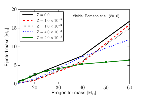
Figure 1: In this figure, we report the ejected mass of oxygen as a function of the progenitor mass, for different initial stellar metallicities. This set of stellar yields is from Romano et al. (2010). The solid line in black corresponds to the stellar yields at $\text{Z}=1.0\times 10^{-10}$; the dashed line in red to $\text{Z}=1.0\times 10^{-5}$; the black dotted line to $\text{Z}=1.0\times 10^{-3}$; the dashed-dotted line in blue to $\text{Z}=3\times 10^{-3}$, and the green squares to the stellar yields at $\text{Z}=2.0\times 10^{-2}$.

Historically, this approach was first used in the early work of Searle & Sargent (1972), who derived the relation between gas phase metallicity Z and gas fraction $\mu=M_{\text{gas}}/(M_{\text{gas}}+M_{\star})$ for a closed box model (see Tinsley 1980, or Matteucci 2001 for a detailed analysis):

$$\text{Z}=y_{\text{Z}}\ln\left(\frac{1}{\mu}\right).$$ (1)

This simple model is based upon the assumptions that the galaxy is one-zone and closed; the initial gas mass is of primordial chemical composition; the initial mass function (IMF) is invariant, and the mixing of the gas in the galaxy is always instantaneous and complete, and that metals are instantaneously recycled for the formation of the new generation of stars. The latter is dubbed “instantaneous recycling approximation” (IRA, Tinsley 1980). Within this simplified (but widely used) approach the further approximation is that all stars with $m\geq 1\,\text{M}_{\sun}$ die instantaneously, while all stars with $m<1\,\text{M}_{\sun}$ have infinite lifetime; this way, the effect of stellar lifetimes in the equations can be neglected and the effect subsumed into a net return fraction ($R$).

Although the IRA assumption is strong, it still represents a good approximation for those chemical elements produced and restored into the ISM by stars with short lifetimes. The best example of such a chemical element is oxygen, which is also representative of the global metallicity Z, since it is the most abundant heavy element by mass. On the other hand, the ISM evolution of chemical elements produced by long-lifetime sources cannot be followed by analytical models working with the IRA assumption. Examples of such chemical elements are nitrogen and carbon, which are mainly synthesized by low- and intermediate-mass stars (LIMS), and iron, mainly produced by Type Ia SNe. To take into account the stellar lifetimes with a high level of detail, numerical models of chemical evolution should be used (see Matteucci 2012).

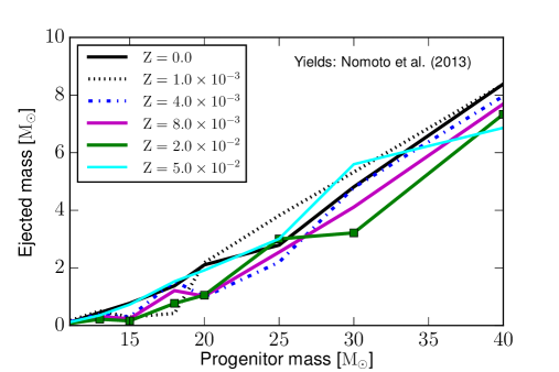
Figure 2: In this figure, we show how ejected mass of oxygen vary as a function of the progenitor mass, for different initial stellar metallicities, when assuming the Nomoto et al. (2013) stellar yields. The solid line in black corresponds to the stellar yields at $\text{Z}=0.0$; the dotted line in black to $\text{Z}=1.0\times 10^{-3}$; the dashed-dotted line in blue to $\text{Z}=4.0\times 10^{-3}$; the solid line in magenta to $\text{Z}=8.0\times 10^{-3}$; the solid line in green to $\text{Z}=2.0\times 10^{-2}$, and the solid line in cyan to the stellar yields at $\text{Z}=5.0\times 10^{-2}$.

The yield per stellar generation is a key in the context of analytical models of chemical evolution, even in the most complex ones, which include the effect of outflows and inflows, as well as variations of the star formation efficiency, i.e. normalization and slope of the relation between gas mass and star formation rate, (see, for example, Bouché et al. 2010; Spitoni et al. 2010; Dekel et al. 2013; Peng & Maiolino 2014; Zahid et al. 2014; Ascasibar et al. 2014; Spitoni 2015), as well as in numerical simulations (e.g. Cole et al. 2000; De Lucia et al. 2004). The comparison of these models with the extensive observations that are providing metallicity measurements for large samples of galaxies locally and at high redshift (e.g. Savaglio et al. 2005; Maiolino et al. 2008; Troncoso et al. 2014; Steidel et al. 2014) enable us to provide important constraints on these various processes, modulo an accurate knowledge of the yield per stellar generation.

In most of the studies, the yield per stellar generation is taken as a fixed value (typically about $0.012$-$0.045$), with this value changing from work to work. For example, a net yield of oxygen $y_{\mathrm{O}}=0.015$ is assumed in Peeples et al. (2014), whereas $y_{\mathrm{O}}=5.7\times 10^{-3}$ in Zahid et al. (2014) and $y_{\mathrm{O}}=3.13\times 10^{-3}$ in Ho et al. (2015); particularly high are the values $y_{\text{O}}=0.040$-$0.045$ assumed in De Lucia et al. (2004), $y_{\text{O}}=0.03$ in Croton et al. (2006), and $y_{\text{O}}=0.04$ in Bower et al. (2008). However, since the net yield is a combination of yields from different stellar masses, it is clear that it must depend on the IMF. This has sometimes been acknowledged (e.g. Henry et al. 2000; Kobayashi et al. 2011; Ho et al. 2015), but never really taken into consideration when using the net yield in the various models. In particular, several works derive the stellar mass and SFR by assuming a given IMF and then adopt a fiducial net yield that is derived from a completely different IMF. Moreover, there is some evidence that the IMF may vary in different classes of galaxies. This implies that different yields per stellar generation should be used. Finally, since the stellar nucleosynthetic yield have a metallicity dependence, it is important to check the effect of metallicity on the IMF-integrated net yield.

To tackle the issues presented above, in this article we calculate yields per stellar generation for the most commonly adopted IMFs and investigate their metallicity dependence (although the latter effect is shown to be minor), by comparing the results for two modern compilations of nucleosynthetic yields (Romano et al., 2010; Nomoto et al., 2013), which have been throughly tested in the past against the best available data for galaxies, although we remark on the fact that each of them is still affected by specific limitations (as discussed in the following Sections). We mostly focus on the yield of oxygen, which is the element which is most commonly used as a tracer of the global metallicity, and for which the IRA approximation is appropriate. However, we will also provide the yield per stellar generation for the total mass of metals, although this should be used with caution, given the enrichment delay of various elements (e.g. iron, nitrogen, carbon, etc…), for which the IRA approximation is arguable.

In Section 2 we define the quantities we have computed in this work and specify the set of stellar yields which we have assumed and the IMFs which we have explored. In Section 3 we report and discuss our results. Finally, in Section 4 we summarize the main conclusions.

2 Definitions and assumptions

2.1 Yield per stellar generation and return mass fraction

We define as yield per stellar generation $y_{i}(\text{Z})$, or net yield, the ratio of the global gas mass in the form of a given chemical element $i$ newly produced and restored into the ISM by a simple stellar population with initial metallicity Z to the amount of mass locked up in low mass stars and stellar remnants (Tinsley, 1980; Maeder, 1992; Matteucci, 2001):

$$y_{i}(\text{Z})=\frac{1}{1-R(\text{Z})}\frac{\int^{m_{\text{up}}}_{m_{\text{long-liv}}}m\,p_{i}(m,\text{Z})\,\phi(m)\,dm}{\int^{m_{\text{up}}}_{0.1~{}\text{M}_{\sun}}m\,\phi(m)\,dm},$$ (2)

where:

1. $p_{i}(m,\text{Z})=\frac{M_{\text{ej},i}(m,\text{Z})}{m}$ is the so-called stellar yield, which is defined such that $m\cdot{p_{i}(m,\text{Z})}$ represents the mass in the form of the $i$-th chemical element newly formed and ejected into the ISM by stars with initial mass $m$ and metallicity Z;

2. $\phi(m)$ is the IMF, namely the mass-spectrum over which the stars of each single stellar generation are distributed at their birth;

3. $m_{\text{long-liv}}=1.0\,\text{M}_{\sun}$ is the maximum mass of the so-called long-lived stars, which do not pollute the ISM;

4. $m_{\text{up}}$ is the upper mass cutoff of the IMF; in our standard case, we assume $m_{\text{up}}=100\,\text{M}_{\sun}$, however in the second part of the article we will also investigate the effect of varying $m_{\text{up}}$.

Finally, $R$ represents the so-called return mass fraction, which is defined as the total mass fraction (including both processed and unprocessed material) returned into the ISM by a stellar generation:

$$R(\text{Z})=\frac{\int^{m_{\text{up}}}_{m_{\text{long-liv}}}(m-M_{R}(m,\text{Z}))\,\phi(m)\,dm}{\int^{m_{\text{up}}}_{0.1~{}\text{M}_{\sun}}m\,\phi(m)\,dm},$$ (3)

with $M_{R}(m,\text{Z})$ being the mass of the stellar remnant left by a stars with initial mass $m$ and metallicity Z.

Table 1: In this Table, we report the numerical values of $\langle P_{\mathrm{O}}\rangle$, which is defined as the IMF-averaged stellar yield of oxygen in the mass range $M=10$-$40\,\mathrm{M}_{\sun}$, for different metallicities Z. ’MM02’ and ’HMM05’ stand for Meynet & Maeder (2002) and Hirschi et al. (2005), respectively, which correspond to the results of the Geneva stellar models also included in Romano et al. (2010). ’NKT13’ stands for Nomoto et al. (2013).

Stellar yields	$v_{\mathrm{rot}}$ [km s-1]	Z	$\langle P_{\mathrm{O}}\rangle$	$\langle P_{\mathrm{O}}\rangle$	$\langle P_{\mathrm{O}}\rangle$	$\langle P_{\mathrm{O}}\rangle$
			Salpeter (1955)	Chabrier (2003)	Kroupa et al. (1993)	Kroupa (2001)
MM02	$0$	$4.0\times 10^{-3}$	$0.004$	$0.007$	$0.002$	$0.007$
	$300$		$0.006$	$0.010$	$0.003$	$0.010$
HMM05	$0$	$2.0\times 10^{-2}$	$0.006$	$0.010$	$0.003$	$0.010$
	$300$		$0.009$	$0.015$	$0.005$	$0.014$
NKT13	no	$4.0\times 10^{-3}$	$0.007$	$0.011$	$0.004$	$0.010$
	no	$2.0\times 10^{-2}$	$0.006$	$0.009$	$0.003$	$0.009$

If one changes the quantity $m_{\text{long-liv}}$ in accordance to the age of the galaxy, then one would obtain equations very similar to the ones numerically solved by current models of chemical evolution (see, for example, Matteucci 2012). In principle, the assumption of $m_{\text{long-liv}}=1.0\,\text{M}_{\sun}$ provides correct results only for stellar populations which are older than $\approx 7.1\,\text{Gyr}$, which corresponds to the lifetime of an $1\,\text{M}_{\sun}$ star, according to Padovani & Matteucci (1993), although the lifetimes of low-mass stars can also be influenced by metallicity, particularly at very low Z (Gibson, 1997).

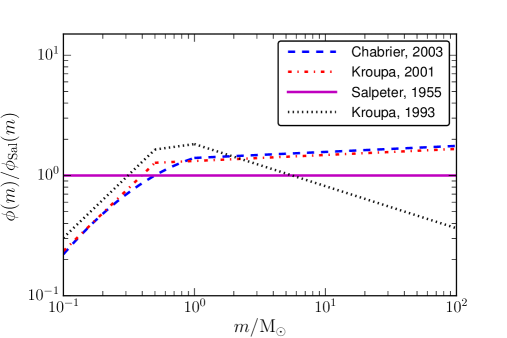
Figure 3: In this figure, we show the trend of the different IMFs studied in this work, as normalized with respect to the Salpeter (1955) IMF. The dotted line in black corresponds to the Kroupa et al. (1993) IMF; the dotted-dashed line in red to the Kroupa (2001) IMF; the dashed line in blue to the Chabrier (2003) IMF, and the solid line in purple corresponds to the Salpeter (1955) IMF.

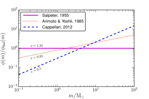
Figure 4: In this figure, we compare the Cappellari et al. (2012, blue dashed line) top-heavy IMF with the IMFs of Arimoto & Yoshii (1987, red dotted line) and Salpeter (1955, solid line in magenta). As in Fig. 3, all the IMFs are normalized with respect to the Salpeter (1955) IMF.

2.2 Stellar yields and initial mass function

We use a numerical code of chemical evolution to explore the effect of the metallicity and IMF on the yields of oxygen per stellar generation and on the return mass fraction. We provide our results for the following sets of stellar yields:

1. the set provided by Romano et al. (2010), which assume the stellar yields of Karakas (2010) for LIM stars, and the He, C, N and O stellar yields of the Geneva stellar models for massive stars (Meynet & Maeder, 2002; Hirschi et al., 2005; Hirschi, 2007; Ekström et al., 2008); for heavier elements, which are not relevant for this study, Romano et al. (2010) assume the stellar yields of massive stars of Kobayashi et al. (2006);

2. the stellar yields of Nomoto et al. (2013), which include the stellar yields of LIM stars of Karakas (2010), and the stellar yields of Nomoto et al. (2006), Kobayashi et al. (2006), Kobayashi et al. (2011), Tominaga et al. (unpublished) for core-collapse supernovae (SNe).

The mass of the stellar remnants have been collected by Romano et al. (2010) from the work of Kobayashi et al. (2006). Nevertheless, according to the Talbot & Arnett (1973) formalism, we compute the return mass fraction with the Romano et al. (2010) stellar yields, by summing the ejecta of all the chemical elements (both the processed and the unprocessed ones) for each stellar mass, and this quantity turns out to be dominated by the H and He contributions.

The Romano et al. (2010) compilation of stellar yields for He, C, N and O include the results of models which take into account the combined effect of mass loss and rotation (see also Maeder 2009 for a detailed discussion), whereas the Nomoto et al. (2013) stellar yields have been computed by models which do include standard mass loss but not the effect of rotation. With standard mass loss, only C and N have been lost before supernova explosions. However, the mass loss driven by rotation turns out to be particularly important at almost solar metallicity and above in depressing the oxygen stellar yields of the most massive stars ($M\ga 30$-$40\,\text{M}_{\sun}$, see also Fig. 1). In fact, mass loss increases with stellar metallicity and stars of high metal content loose H, He, but also C, through radiatively line driven winds. Therefore, the C production is increased by mass loss whereas the oxygen production is decreased, since part of C which would have been transformed into O, is lost from the star (Maeder, 1992). Finally, the effect of rotation is to produce mixing and enhances mass loss, with the efficiency of the mixing process being larger at lower metallicities (see also Chiappini et al. 2008, and references therein).

We remark on the fact that Romano et al. (2010) combine results of stellar models assuming only hydrostatic burning and rotation (Geneva group, for He, C, N, and O) with the results of models including explosive burning without rotation (Nomoto group, for heavier elements), giving rise to an inhomogeneous set of stellar yields, which can be physically incorrect. In the context of this study, the treatment of Romano et al. (2010) has a marginal effect, since the metallicity is dominated by the oxygen and carbon contributions. On the other hand, Nomoto et al. (2013) provide one of the most homogeneous set of stellar yields available at the present time, although it is still affected by the limitation of not including the effect of stellar rotation.

In Figures 1 and 2, we show how the oxygen stellar yields of Romano et al. (2010) and Nomoto et al. (2013), respectively, vary as functions of the initial stellar mass and for different metallicities. The Geneva stellar yields are available only up $60\,\text{M}_{\sun}$ and we therefore assume in our standard case that the yields from $60$ to $100\,\text{M}_{\sun}$ are constant. On the other hand, the stellar yields of massive stars of Kobayashi et al. (2006, included in , for the elements heavier than oxygen) and Nomoto et al. (2013) are available only up to $40\,\text{M}_{\sun}$ and thus we keep them constant for stars with larger initial mass. We remark on the fact that very massive stars are expected to leave a black hole as a remnant; therefore, a significant fraction of stellar nucleosythetic products in the ejecta of very massive stars may eventually fall back onto the black hole. This process might cause a reduction of the stellar yields of very massive stars.

At solar metallicity, Romano et al. (2010) include stellar yields which have been computed by applying a stellar rotational velocity $v_{\mathrm{rot}}=300$ km s^-1. From an observational point of view, Ramírez-Agudelo et al. (2013) found that almost $80$ per cent of nearby stars rotate slower than $v_{\mathrm{rot}}=300$ km s^-1, which thus can be considered as an approximate upper limit. To quantify the effect of stellar rotation in the stellar yields of oxygen from massive stars, in Table 1 we compare the predictions of models with and without stellar rotation, with the quantity $\langle P_{\mathrm{O}}\rangle$ being defined as the IMF-averaged yield of oxygen in the mass range $M=10$-$40\,\mathrm{M}_{\sun}$. The effect of stellar rotation in the Geneva stellar models is to increase the average oxygen stellar yield by a factor of $\sim 1.5$ for stars with initial mass below $40\,\mathrm{M}_{\sun}$ (see also Hirschi et al. 2005). Furthermore, at $\mathrm{Z}=4.0\times 10^{-3}$, the IMF-averaged oxygen stellar yield of Nomoto et al. (2013) – which neglect the effect of stellar rotation – is larger than the value of the Geneva stellar models without stellar rotation, but rather similar to the corresponding value with rotation; conversely, at solar metallicity, the Geneva stellar models without rotation agree with Nomoto et al. (2013). IMFs containing a larger number of massive stars, such as the Chabrier (2003) and Kroupa (2001) ones, amplify the oxygen enrichment of the ISM and give rise to larger values of $\langle P_{\mathrm{O}}\rangle$, whatever be the set of stellar yields assumed.

In this article, we study the effect of different IMFs: the Salpeter (1955), the Kroupa et al. (1993), the Kroupa (2001), and the Chabrier (2003) IMFs, which are shown in Fig. 3 as normalized with respect to the Salpeter (1955) IMF. We have chosen these IMFs since they have been the most widely used by various authors. Moreover, these IMFs give quite different weights to different stellar mass ranges, hence they will more clearly display differences in the final predicted net yields and return mass fractions. As one can notice from Fig. 3, the Kroupa et al. (1993) IMF predicts the largest fraction of intermediate mass stars, while having the lowest number of massive stars. On the other hand, the Chabrier (2003) and the Kroupa (2001) IMFs predict a higher number of both intermediate-mass stars and massive stars than the Salpeter (1955) IMF.

Finally, we also explore the effect of the top-heavy IMFs of Cappellari et al. (2012) and Arimoto & Yoshii (1987), which are shown in Fig. 4, as normalized with respect to the Salpeter (1955) IMF. These IMFs are defined as a single-slope power law: $\phi(m)\propto m^{-(1+x)}$, with the Cappellari et al. (2012) IMF having a slope $x=0.5$ and the Arimoto & Yoshii (1987) IMF assuming $x=0.95$.

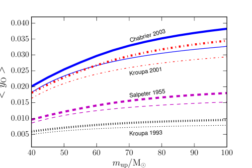
Figure 5: In this figure, we show how $\langle y_{\text{O}}\rangle$ is predicted to vary as a function of $m_{\text{up}}$, which is defined as the upper mass cutoff of the IMF. We have computed $\langle y_{\text{O}}\rangle$, by averaging the net yield of oxygen over the metallicity range $1.0\times 10^{-3}\leq\text{Z}\leq 2.0\times 10^{-2}$, within which $y_{\text{O}}$ turns out to be nearly constant. Thick lines represent our results for the Romano et al. (2010) stellar yields, while thin lines represent the Nomoto et al. (2013) stellar yields. The various curves with different colours correspond to the same IMFs as in Fig. 3.

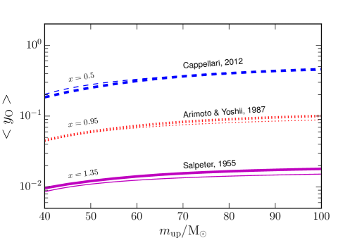
Figure 6: In this figure, we report how the average net yield of oxygen, $\langle y_{\text{O}}\rangle$, varies as a function of the upper cutoff of the IMF, when assuming the top-heavy IMF of Cappellari et al. (2012, blue dashed line) and the IMFs of Arimoto & Yoshii (1987, red dotted line) and Salpeter (1955, solid line in magenta). As in Fig. 5, $\langle y_{\text{O}}\rangle$ is computed by averaging $y_{\text{O}}$ over the metallicity range $1.0\times 10^{-3}\leq\text{Z}\leq 2.0\times 10^{-2}$, and the various curves with different thickness correspond to the same stellar yields as in Fig. 5.

3 Results

In this Section we present the net nucleosynthetic yields and return fractions obtained with the IMFs and stellar yields discussed in the previous section. As mentioned above, we will focus on the yield of oxygen, since it is the element most commonly measured and taken as representative of the bulk of the metallicity, and also because it is an element for which the IRA approximation is appropriate. However, we will provide a value also for the yield of the total mass of metals, although with some cautionary warnings.

Table 2: In this Table, we report the numerical values which we predict for the return mass fraction ($R$) and the yields of oxygen and metals per stellar generation ($y_{\text{O}}$ and $y_{\text{Z}}$, respectively) as functions of the metallicity Z and for different IMFs. These values have been computed by assuming that the upper mass cutoff of the IMF $m_{\text{up}}=100\,\text{M}_{\sun}$. The stellar yields are the ones of Romano et al. (2010).

Stellar yields: Romano et al. (2010)
Z	$R$	$y_{\text{O}}$	$y_{\text{Z}}$	$R$	$y_{\text{O}}$	$y_{\text{Z}}$	$R$	$y_{\text{O}}$	$y_{\text{Z}}$	$R$	$y_{\text{O}}$	$y_{\text{Z}}$
	IMF: Salpeter (1955)			IMF: Chabrier (2003)			IMF: Kroupa et al. (1993)			IMF: Kroupa (2001)
$1.0\times 10^{-10}$	$0.285$	$0.028$	$0.042$	$0.436$	$0.059$	$0.088$	$0.284$	$0.015$	$0.026$	$0.411$	$0.053$	$0.079$
$1.0\times 10^{-5}$	$0.285$	$0.018$	$0.028$	$0.436$	$0.039$	$0.059$	$0.284$	$0.009$	$0.017$	$0.411$	$0.035$	$0.053$
$5.0\times 10^{-5}$	$0.285$	$0.018$	$0.028$	$0.436$	$0.039$	$0.059$	$0.284$	$0.009$	$0.017$	$0.411$	$0.035$	$0.053$
$1.0\times 10^{-4}$	$0.285$	$0.018$	$0.029$	$0.436$	$0.039$	$0.060$	$0.284$	$0.009$	$0.018$	$0.411$	$0.035$	$0.054$
$5.0\times 10^{-4}$	$0.286$	$0.018$	$0.029$	$0.437$	$0.039$	$0.060$	$0.285$	$0.009$	$0.018$	$0.412$	$0.035$	$0.054$
$1.0\times 10^{-3}$	$0.286$	$0.018$	$0.029$	$0.438$	$0.039$	$0.060$	$0.287$	$0.009$	$0.017$	$0.414$	$0.035$	$0.054$
$5.0\times 10^{-3}$	$0.292$	$0.018$	$0.027$	$0.447$	$0.038$	$0.057$	$0.295$	$0.009$	$0.016$	$0.422$	$0.034$	$0.051$
$1.0\times 10^{-2}$	$0.295$	$0.018$	$0.028$	$0.451$	$0.038$	$0.060$	$0.299$	$0.010$	$0.017$	$0.425$	$0.034$	$0.054$
$2.0\times 10^{-2}$	$0.298$	$0.018$	$0.031$	$0.455$	$0.037$	$0.065$	$0.302$	$0.010$	$0.018$	$0.430$	$0.034$	$0.059$

In Table 2, we show how the net yield of oxygen per stellar generation varies as a function of the IMF and metallicity. In our “fiducial” case, reported in Table 2, we assume $m_{\text{up}}=100\,\text{M}_{\sun}$. Concerning the dependence on metallicity, the most interesting result is that the yield $y_{\text{O}}$ is roughly constant down to very low metallicities. This result implies that the assumption of a time-independent net oxygen yield, as generally treated in analytical models, is a reasonable one. Interestingly, we find an enhancement of $y_{\text{O}}$ for metal-free stellar populations (case with $Z=1.0\times 10^{-10}$ from Ekström et al. 2008). In fact, it is well established that, at very low Z, the mixing induced by rotation is particularly efficient (Chiappini et al., 2008); in this way, the nucleosynthetic products of the $3\alpha$ reaction in the inner He-burning zone can diffuse to the outer stellar zones, so that radiative winds and mass loss (boosted by the high surface enrichment in heavy elements) are highly enriched with the CNO elements; this cannot be obtained by models of metal-free non-rotating massive stars (see, for example, Maeder 2009, for a detailed discussion).

On the other hand, $y_{\text{O}}$ is strongly dependent on the assumed IMF. The highest oxygen yield is obtained when adopting a Chabrier (2003) IMF, because this particular IMF contains the largest number of massive stars compared to the other IMFs explored in this paper (see Fig. 3). The IMF of Kroupa et al. (1993), instead, predicts the lowest $y_{\text{O}}$, since it contains the lowest fraction of high mass stars. In this context, it is important to distinguish the two IMFs suggested by Kroupa. In fact the Kroupa (2001) is very similar to the IMF of Chabrier (2003) and predicts a substantially higher yield than Kroupa et al. (1993). The Salpeter (1955) IMF predicts a net yield roughly halfway between the Chabrier (2003) and Kroupa et al. (1993) IMFs.

In Table 2, we show also how $y_{\text{Z}}$ (where Z here is the sum of all metals) is predicted to vary as a function of the different IMFs and metallicities. These values are shown here only for reference with previous works attempting to model the total metal content of galaxies, however we caution the reader against a blind application of analytical models assuming the IRA to the total metal content. Finally, in the same Table, we report the values of the returned fraction $R$, which is rather constant as a function of metallicity but shows some change for different IMFs. The approximate constancy of $R$ as a function of the metallicity is due to the fact that this quantity is strongly dominated by the H and He contributions.

Our results for $y_{\text{O}}(\text{Z})$, $y_{\text{Z}}(\text{Z})$ and $R(\text{Z})$, as obtained with the Nomoto et al. (2013) set of stellar yields, are reported in Table 3. The effect of the various IMFs is the same as discussed above for the stellar yields of Romano et al. (2010, see Table 2). On the other hand, by comparing the predicted net yields of metals and oxygen of Romano et al. (2010) with the ones of Nomoto et al. (2013), we can quantify the uncertainty introduced by different input stellar yields by a factor which is $\sim 1.5$.

Table 3: In this Table, we report the numerical values which we predict for the return mass fraction ($R$) and the yields of oxygen and metals per stellar generation ($y_{\text{O}}$ and $y_{\text{Z}}$, respectively) as functions of the metallicity Z and for different IMFs. These values have been computed by assuming that the upper mass cutoff of the IMF $m_{\text{up}}=100\,\text{M}_{\sun}$. The stellar yields are the ones of Nomoto et al. (2013).

Stellar yields: Nomoto et al. (2013)
Z	$R$	$y_{\text{O}}$	$y_{\text{Z}}$	$R$	$y_{\text{O}}$	$y_{\text{Z}}$	$R$	$y_{\text{O}}$	$y_{\text{Z}}$	$R$	$y_{\text{O}}$	$y_{\text{Z}}$
	IMF: Salpeter (1955)			IMF: Chabrier (2003)			IMF: Kroupa et al. (1993)			IMF: Kroupa (2001)
$0.0$	$0.261$	$0.021$	$0.043$	$0.403$	$0.044$	$0.087$	$0.244$	$0.011$	$0.024$	$0.380$	$0.040$	$0.079$
$1.0\times 10^{-3}$	$0.293$	$0.018$	$0.026$	$0.450$	$0.038$	$0.055$	$0.291$	$0.009$	$0.014$	$0.424$	$0.034$	$0.050$
$5.0\times 10^{-3}$	$0.300$	$0.016$	$0.025$	$0.459$	$0.034$	$0.052$	$0.300$	$0.008$	$0.013$	$0.433$	$0.030$	$0.047$
$1.0\times 10^{-2}$	$0.302$	$0.015$	$0.024$	$0.463$	$0.032$	$0.051$	$0.303$	$0.008$	$0.013$	$0.436$	$0.029$	$0.046$
$2.0\times 10^{-2}$	$0.305$	$0.014$	$0.023$	$0.466$	$0.030$	$0.049$	$0.307$	$0.007$	$0.012$	$0.439$	$0.027$	$0.044$
$5.0\times 10^{-2}$	$0.304$	$0.017$	$0.023$	$0.466$	$0.036$	$0.049$	$0.307$	$0.009$	$0.012$	$0.439$	$0.032$	$0.044$

In Fig. 5, we explore how the choice of the upper cutoff of the IMF, $m_{\text{up}}$, affects the average net yield of oxygen, where $\langle y_{\text{O}}\rangle$ stands for the net yield of oxygen as averaged in the metallicity range $1.0\times 10^{-3}\leq\text{Z}\leq 2.0\times 10^{-2}$. Our results are shown for different IMFs (different colors) and different stellar yield compilations (thick and thin lines represent our results with Romano et al. 2010 and Nomoto et al. 2013, respectively). By looking at the figure, we see that the difference between the case with $m_{\text{up}}=100\,\text{M}_{\sun}$ and $m_{\text{up}}=40\,\text{M}_{\sun}$ is as much as a factor of about two. The difference is only $\sim 50$ per cent between $m_{\text{up}}=100\,\text{M}_{\sun}$ and $m_{\text{up}}=60\,\text{M}_{\sun}$. We find that, when assuming the Chabrier (2003) and Kroupa et al. (1993) IMFs, the differences in $\langle y_{\text{O}}\rangle$ with different upper mass limits are almost doubled and halved, respectively, with respect to the case with the Salpeter (1955). Fig. 5 shows that the global variation of $\langle y_{\text{O}}\rangle$ spanned by all “classical” IMFs and the possible range of $m_{\text{up}}$ is nearly a factor of ten.

By looking at Fig. 5, the curves corresponding to the Romano et al. (2010) stellar yields lie always above the curves with the Nomoto et al. (2013) stellar yields. This difference enlarges as $m_{\text{up}}$ increases, because Romano et al. (2010) provide the oxygen stellar yields up to $60\,\text{M}_{\sun}$, while Nomoto et al. (2013) only up to $40\,\text{M}_{\sun}$ (see also Fig. 1), and we keep these stellar yields constant for stars with larger initial stellar mass. The latter assumption can introduce a systematic effect in the final values of $y_{\text{O}}$. We find that, by varying the upper limit of the integral at the numerator of equation 2 and by normalizing the IMF up to $m_{\text{up}}=100\,\text{M}_{\sun}$, the trend of the resulting $\langle y_{\text{O}}\rangle$ is similar to the trend of $\langle y_{\text{O}}\rangle$ as a function of the upper cutoff of the IMF (see Fig. 5).

Assuming a top-heavy IMF can cause an even larger increase of the yield of oxygen per stellar generation, being larger the number of massive stars which are present. We explore the effect of two top-heavy IMFs (Cappellari et al., 2012; Arimoto & Yoshii, 1987), both defined as a single-slope power law. Our results for the $\langle y_{\text{O}}\rangle$ vs. $m_{\mathrm{up}}$ relations are shown in Fig. 6 for different IMFs and stellar yield assumptions. By looking at Fig. 6, as the slope of the IMF is decreased from $x=1.35$ (Salpeter, 1955) down to $x=0.95$ (Arimoto & Yoshii, 1987) and $x=0.5$ (Cappellari et al., 2012), the IMF becomes top-heavier and the value of $y_{\mathrm{O}}$ becomes larger and larger; furthermore, the standard deviation of $\langle y_{\text{O}}\rangle$ becomes larger as the slope $x$ is decreased, indicating that $\langle y_{\text{O}}\rangle$ is slightly more influenced by the metallicity-dependence of the assumed set of stellar yields.

The predicted values of $y_{\mathrm{O}}$ for single-slope top-heavy IMFs are very high and they may either imply that a top-heavy IMF star formation mode has only lasted for a short interval of the galaxy lifetime and not relevant for the integrated metal production, or that a single power-law is not a proper representation of the “top-heavy IMF” and that a broken power-law is a more proper description.

There is increasing evidence in the literature that the IMF may vary among different types of stellar systems, such as spheroids and disk galaxies, as well as faint dwarf galaxies (e.g. see Cappellari et al. 2012; Conroy & van Dokkum 2012; Weidner et al. 2013). Observationally, a Kroupa et al. (1993) IMF is favoured in describing the chemical evolution of the solar vicinity (see Romano et al. 2010), and the disk of spirals similar to the Milky Way, while the Kroupa (2001) and Chabrier (2003) IMFs are probably better for describing the evolution of spheroids such as bulges and ellipticals (see, for example, Chabrier et al. 2014). We have shown that the range of commonly adopted IMFs (even neglecting the extreme top-heavy IMFs) implies a large variation of net yield per stellar generation. This fact could add an extra systematic to studies attempting to model the observed abundances, which should be taken into account by properly using our compilation of yield for the different classes of galaxies. More specifically, if the IMF is not universal, we can expect a difference in net yield up to a factor larger than three for classical, widely-used IMFs, and even much larger for top-heavy IMFs.

4 Conclusions and discussion

The blooming of extensive spectroscopic surveys of local and distant galaxies have fostered the use of metallicities to constrain the star formation history, feedback processes (outflows) and gas inflows across the cosmic epoch, by comparing the observations with the expectations of analytical and numerical models. One key element in such a comparison is the yield per stellar generation, which is often assumed as a fixed value. In this article, we have used a numerical code of chemical evolution, which includes modern stellar nucleosynthetic yields, to explore the effect of the metallicity and IMF on the net yield of oxygen per stellar generation and on the return mass fraction; our results have shown that the yield can change by large factors. Therefore, if the yield associated with the appropriate IMF is not used, this can produce inconsistent results and large systematic errors.

We have provided results for two different sets of stellar yields, which are Romano et al. (2010) and Nomoto et al. (2013). The former is an inhomogeneous set, since it combines results of hydrostatic burning in rotating massive stars (He, C, N, and O from Geneva stellar models) with results of explosive burning without stellar rotation (heavier elements from Kobayashi et al. 2006), which is – in principle – an incorrect treatment. On the other hand, Nomoto et al. (2013) is a homogeneous set of stellar yields, with the only limitation of not including the effect of stellar rotation, expected to have a strong impact at the very low metallicities. We have found that the uncertainty introduced by assuming different sets of stellar yields can be quantified by $\sim 0.2\,\text{dex}$.

The effect of assuming different IMFs can cause large differences in the net oxygen yield. We have found that the Kroupa (2001) and Chabrier (2003) predict the highest oxygen yield, roughly a factor of two higher than for a Salpeter (1955) IMF. On the other hand, by assuming a Kroupa et al. (1993) IMF, we obtain the smallest net yield, roughly a factor of two lower than for a Salpeter (1955) IMF.

The yield per stellar generation also depends significantly on the upper mass cutoff of the IMF. The differences between the case with $m_{\text{up}}=100\,\text{M}_{\sun}$ and $m_{\text{up}}=40\,\text{M}_{\sun}$ are of the order of a factor of two with the Salpeter (1955). Since the IMF of Chabrier (2003) predicts a larger number of massive stars, that difference is doubled with this IMF, whereas it is halved with the Kroupa et al. (1993) IMF, which predicts the lowest number of massive stars. If one takes into account both the variation with IMF shape and upper stellar mass cutoff, the variation of the yield per stellar generation can span more than a factor of ten.

We note that populations of highly enriched galaxies – whose metallicities were deemed uncomfortably high – can be easily explained by means of a large yield per stellar generation, as the one associated with commonly used IMFs, such as Chabrier (2003) and Kroupa (2001). Similarly, our results should warn about a proper use of the so-called effective yield, $y_{\text{eff}}=\text{Z}/\ln\left(\mu^{-1}\right)$, which is observationally derived by inverting equation (1). In particular, the finding of $y_{\text{eff}}<y_{\text{Z}}$ is generally modelled in terms of enriched outflows, inflow of pristine gas, or both (e.g. Tremonti et al. 2004; Erb 2008; Mannucci et al. 2009; Troncoso et al. 2014), whereas the finding of $y_{\text{eff}}>y_{\text{Z}}$ is sometimes used as an indicator of inaccurate metallicity measurements or inappropriate metallicity calibrations. We conclude that the deviation of $y_{\text{eff}}$ from a “fiducial”, “true” yield also may be partly associated with IMF being different than assumed. For the same reason, high values of the the effective yield (and in particular $y_{\text{eff}}>y_{\text{Z}}$) may be indicative of an IMF favouring massive stars (Chabrier, 2003; Kroupa, 2001) and/or of an high mass cutoff of the IMF itself. By assuming single-slope top-heavy IMFs, such as the ones proposed by Arimoto & Yoshii (1987) or Cappellari et al. (2012), we find very high values for the yields of oxygen per stellar generation, which are also slightly influenced by the metallicity-dependence of the stellar yields.

The dependence on metallicity of the yield is reassuringly small. A significant variation is only found at extremely low metallicities ($\text{Z}=1.0\times 10^{-10}$). Although the latter result may be an important aspect to take into account for models of primordial galaxies, it strongly relies on the assumed set of stellar yields, which are particularly affected by uncertainties at extremely low metallicities.

We remind the reader that IRA provides correct results only for chemical elements restored into the ISM on short typical time-scales; oxygen represents the best example of such a chemical element, since it is also the most abundant metal by mass in the Universe. On the other hand, analytical models working under IRA assumption fail in following the evolution of chemical elements produced by long-lifetime sources; examples of such chemical elements are carbon, nitrogen and iron. Hence we warn the reader against a blind application of IRA for the total mass of metals. In order to take into account the lifetimes of the various stellar producers in detail, numerical models of chemical evolution should be used.

Our compilation of numerical values of the yield per stellar generation, for different IMFs, different upper mass cutoffs and different metallicities, will hopefully be useful to properly investigate the metallicity in galaxies across cosmic epochs, by tackling one of the (generally not acknowledged) major sources of uncertainty.

References

- Arimoto & Yoshii (1987) Arimoto N., Yoshii Y., 1987, A&A, 173, 23
- Ascasibar et al. (2014) Ascasibar Y., Gavilán M., Pinto N., et al., 2014, preprint (arXiv:1406.6397)
- Asplund et al. (2009) Asplund M., Grevesse N., Sauval A. J., Scott P., 2009, ARA&A, 47, 481
- Berg et al. (2012) Berg D. A., Skillman E. D., Marble A. R., et al., 2012, ApJ, 754, 98
- Bouché et al. (2010) Bouché N., Dekel A., Genzel R., et al., 2010, ApJ, 718, 1001
- Bower et al. (2008) Bower R. G., McCarthy I. G., Benson A. J., 2008, MNRAS, 390, 1399
- Cappellari et al. (2012) Cappellari M., McDermid R. M., Alatalo K., et al., 2012, Nature, 484, 485
- Chabrier (2003) Chabrier G., 2003, PASP, 115, 763
- Chabrier et al. (2014) Chabrier G., Hennebelle P., Charlot S., 2014, ApJ, 796, 75
- Chiappini et al. (2008) Chiappini C., Ekström S., Meynet G., et al., 2008, A&A, 479, L9
- Cole et al. (2000) Cole S., Lacey C. G., Baugh C. M., Frenk C. S., 2000, MNRAS, 319, 168
- Conroy & van Dokkum (2012) Conroy C., van Dokkum P. G., 2012, ApJ, 760, 71
- Croton et al. (2006) Croton D. J., Springel V., White S. D. M., et al., 2006, MNRAS, 365, 11
- Davé et al. (2012) Davé R., Finlator K., Oppenheimer B. D., 2012, MNRAS, 421, 98
- Dekel et al. (2013) Dekel A., Zolotov A., Tweed D., et al., 2013, MNRAS, 435, 999
- De Lucia et al. (2004) De Lucia G., Kauffmann G., White S. D. M., 2004, MNRAS, 349, 1101
- Edmunds (1990) Edmunds M. G., 1990, MNRAS, 246, 678
- Edmunds & Greenhow (1995) Edmunds M. G., Greenhow R. M., 1995, MNRAS, 272, 241
- Erb (2008) Erb D. K., 2008, ApJ, 674, 151
- Ekström et al. (2008) Ekström S., Meynet G., Chiappini C., Hirschi R., Maeder A., 2008, A&A, 489, 685
- Gibson (1997) Gibson B. K., 1997, MNRAS, 290, 471
- Henry et al. (2000) Henry R. B. C., Edmunds M. G., Köppen J., 2000, ApJ, 541, 660
- Hirschi et al. (2004) Hirschi R., Meynet G., Maeder A., 2004, A&A, 425, 649
- Hirschi et al. (2005) Hirschi R., Meynet G., Maeder A., 2005, A&A, 433, 1013
- Hirschi (2007) Hirschi R., 2007, A&A, 461, 571
- Ho et al. (2015) Ho I.-T., Kudritzki R.-P., Kewley L. J., et al., 2015, MNRAS, 448, 2030
- Karakas (2010) Karakas A. I., 2010, MNRAS, 403, 1413
- Kobayashi et al. (2006) Kobayashi C., Umeda H., Nomoto K., Tominaga N., Ohkubo T., 2006, ApJ, 653, 1145
- Kobayashi et al. (2011) Kobayashi C., Karakas A. I., Umeda H., 2011, MNRAS, 414, 3231
- Kroupa et al. (1993) Kroupa P., Tout C. A., Gilmore G., 1993, MNRAS, 262, 545
- Kroupa (2001) Kroupa P., 2001, MNRAS, 322, 231
- Lilly et al. (2013) Lilly S. J., Carollo C. M., Pipino A., Renzini A., Peng Y., 2013, ApJ, 772, 119
- Maeder (1992) Maeder A., 1992, A&A, 264, 105
- Maeder et al. (2006) Maeder A., Meynet G., Hirschi R., Ekström S., 2006, Chemical Abundances and Mixing in Stars in the Milky Way and its Satellites, 308
- Maeder (2009) Maeder A., 2009, Physics, Formation and Evolution of Rotating Stars, Astronomy and Astrophysics Library. ISBN 978-3-540-76948-4. Springer Berlin Heidelberg, 2009
- Maiolino et al. (2008) Maiolino R., Nagao T., Grazian A., et al., 2008, A&A, 488, 463
- Mannucci et al. (2009) Mannucci F., Cresci G., Maiolino R., et al., 2009, MNRAS, 398, 1915
- Matteucci & Chiosi (1983) Matteucci F., Chiosi C., 1983, A&A, 123, 121
- Matteucci (2001) Matteucci F., 2001, Astrophysics and Space Science Library, 253
- Matteucci (2012) Matteucci F., 2012, Chemical Evolution of Galaxies: , Astronomy and Astrophysics Library. ISBN 978-3-642-22490-4. Springer-Verlag Berlin Heidelberg, 2012,
- Meynet & Maeder (2002) Meynet G., Maeder A., 2002, A&A, 390, 561
- Meynet et al. (2010) Meynet G., Hirschi R., Ekstrom S., et al., 2010, IAU Symposium, 265, 98
- Nomoto et al. (2006) Nomoto K., Tominaga N., Umeda H., Kobayashi C., & Maeda K., 2006, Nuclear Physics A, 777, 424
- Nomoto et al. (2013) Nomoto K., Kobayashi C., Tominaga N., 2013, ARA&A, 51, 457
- Padovani & Matteucci (1993) Padovani P., Matteucci F., 1993, ApJ, 416, 26
- Peeples et al. (2014) Peeples M. S., Werk J. K., Tumlinson J., et al., 2014, ApJ, 786, 54
- Peng & Maiolino (2014) Peng Y. J., Maiolino R., 2014, MNRAS, 443, 3643
- Ramírez-Agudelo et al. (2013) Ramírez-Agudelo O. H., Simón-Díaz S., Sana H., et al., 2013, A&A, 560, A29
- Recchi & Kroupa (2015) Recchi S., Kroupa P., 2015, MNRAS, 446, 4168
- Romano et al. (2010) Romano D., Karakas A. I., Tosi M., Matteucci F., 2010, A&A, 522, A32
- Salpeter (1955) Salpeter E. E., 1955, ApJ, 121, 161
- Savaglio et al. (2005) Savaglio S., Glazebrook K., Le Borgne D., et al., 2005, ApJ, 635, 260
- Searle & Sargent (1972) Searle L., Sargent W. L. W., 1972, ApJ, 173, 25
- Spitoni et al. (2010) Spitoni E., Calura F., Matteucci F., Recchi S., 2010, A&A, 514, AA73
- Spitoni (2015) Spitoni E., 2015, MNRAS, 451, 5609
- Steidel et al. (2014) Steidel C. C., Rudie G. C., Strom A. L., et al., 2014, ApJ, 795, 165
- Talbot & Arnett (1973) Talbot R. J. Jr., Arnett W. D., 1973, ApJ, 186, 51
- Tinsley (1980) Tinsley B. M., 1980, Fundamentals of Cosmic Physics, 5, 287
- Tremonti et al. (2004) Tremonti C. A., Heckman T. M., Kauffmann G., et al., 2004, ApJ, 613, 898
- Troncoso et al. (2014) Troncoso P., Maiolino R., Sommariva V., et al., 2014, A&A, 563, AA58
- Weidner et al. (2013) Weidner C., Kroupa P., Pflamm-Altenburg J., Vazdekis A., 2013, MNRAS, 436, 3309
- Zahid et al. (2014) Zahid H. J., Dima G. I., Kudritzki R. P., et al., 2014, ApJ, 791, 130