Direct detection of dark matter with resonant annihilation

Abstract

In the scenario where the dark matter (DM) particles $\chi\bar{\chi}$ pair annihilate through a resonance particle $R$, the constraint from DM relic density makes the corresponding cross section for DM-nuclei elastic scattering extremely small, and can be below the neutrino background induced by the coherent neutrino-nuclei scattering, which makes the DM particle beyond the reach of the conventional DM direct detection experiments. We present an improved analytical calculation of the DM relic density in the case of resonant DM annihilation for $s$- and $p$-wave cases and invesitgate the condition for the DM-nuclei scattering cross section to be above the neutrino background. We show that in Higgs-portal type models, for DM particles with $s$-wave annihilation, the spin-independent DM-nucleus scattering cross section is proportional to $\Gamma_{R}/m_{R}$, the ratio of the decay width and the mass of $R$. For a typical DM particle mass $\sim 50$ GeV, the condition leads to $\Gamma_{R}/m_{R}\gtrsim\mathcal{O}(10^{-4})$. In $p$-wave annihilation case, the spin-independent scattering cross section is insensitive to $\Gamma_{R}/m_{R}$, and is always above the neutrino background, as long as the DM particle is lighter than the top quark. The real singlet DM model is discussed as a concrete example.

1 Introduction

Dark matter (DM) contributes to 26.8% of the total energy density of the Universe [1], yet its particle nature remains largely unknown. The leading candidates for DM are weakly interacting massive particles (WIMPs). WIMPs can naturally obtain the observed relic density, and the predicted cross sections of the WIMP-nuclei scattering are usually within the reach of the current DM direct detection experiments. In the case where the DM annihilation cross section times the relative velocity $\sigma v_{\rm rel}$ is a constant, such as that in the simple $s$-wave annihilation cases, the DM relic density can be calculated analytically using the standard freeze-out approximation. The connection between the DM relic density and the DM-nuclei scattering cross section can be straightforwardly established.

However, in many DM models and DM interaction mechanisms, the velocity dependence of $\sigma v_{\rm rel}$ can be complicated. For instance, to explain both the relic density and the cosmic-ray positron excess observed by PAMELE [2], Fermi-LAT [3], and AMS-02 [4, 5], the mechanism of Sommerfeld enhancement has been invoked, which introduces a velocity-dependent DM annihilation cross section [6, 7, 8, 9, 10, 11, 12, 13] to account for the larger cross section required by the data [14, 15, 16].

In a wide class of DM models, the DM particle $\chi$ can annihilate into the standard model (SM) particles through an $s$-channel resonance particle $R$. Such as the singlet scalar DM models [17, 18, 19, 20, 21, 22, 23, 24, 25, 26] , the left-right symmetric models with extended stable scalar sectors [27, 28, 29, 30, 31, 32, 33, 34] and the fermionic DM models [35, 36, 37, 38, 39, 40, 41]. The presence of the scalar $R$ can also play an important role in electroweak phase transion [24, 42, 43, 44, 45, 46, 47, 48, 49, 50, 39] and modify the interpretation of the DM-nuclei scattering [51, 52].

Near the resonance point the kinetic energy of the DM particles is non-negligible, which makes $\sigma v_{\rm rel}$ velocity dependent, and leads to the enhancement of DM annihilation cross section at lower tempertures, the so called Breit-Wigner enhancement[53, 54]. In the scenario of resonant dark matter (DM) annihilation, under the constraint of DM relic density, the cross section for DM-nuclei elastic scattering can be extremely small such that it can fall below the background induced by the coherent neutrino-nuclei scattering, which make it undetectable by the current DM direct detection technology. It is of importance to know under what condition this phenomena will occur. In order to establish the correlation between the DM relic density and the DM-nuclei scattering cross section, it is useful to have analytical expressions for both quantities, which is however challenging, due to the complicated velocity dependence of the DM annihilation cross section in the case with resonance.

The Boltzmann equation which governs the evolution of the DM number density is usually solved analytically by using the standard freeze-out approximation [55]. However, when DM annihilation takes place near a pole in the cross section, we cannot use the standard method as $\langle\sigma v_{\rm rel}\rangle$ does not have a simple analytical form [56]. In Ref. [57], it was proposed to analytically calculate $\langle\sigma v_{\rm rel}\rangle$ using the $\delta$-function approximation, if the resonance has a very narrow decay width. But this method fails in the case where the DM mass is greater than a half of the mass of the resonant particle, namely, above the resonance.

In this work, we present an improved analytical calculation of the DM relic density in the case of resonant DM annihilation for $s$- and $p$-wave cases and investigate the condition for the DM-nuclei scattering cross section to be above the neutrino background. We show that in Higgs-portal type models, for DM particles with $s$-wave annihilation, the spin-independent DM-nucleus scattering cross section is proportional to $\Gamma_{R}/m_{R}$, the ratio of the decay width and the mass of $R$. For a typical DM particle mass $\sim 50$ GeV, the condition leads to $\Gamma_{R}/m_{R}\gtrsim\mathcal{O}(10^{-4})$. In $p$-wave annihilation case, the spin-independent scattering cross section is insensitive to $\Gamma_{R}/m_{R}$, and is always above the neutrino background, as long as the DM particle is lighter than the top quark. As an example, we calculate the spin-independent cross section both analytically and numerically in the real singlet DM model with resonant annihilation. We show that the predicted cross section in this model is always above the neutrino background. In order to cover the full parameter space of this model, the required sensitivity should reach $\sim 2.6\times 10^{-49}~{}{\rm cm^{2}}$ for the next generation direct detection experiments.

This paper is organized as follows: In Sec. 2, we outline the freeze-out approximation of Boltzmann equation, and propose an approximate formula for the relic density of a scalar or fermion DM particle which annihilates through an s-channel scalar resonance which has a narrow decay width. In Sec. 3, we analyse the constraint of neutrino backgroud has on DM direct detection experiments on the resonance point. In Sec. 4, we analyse the direct detection of the real singlet DM. Some discussions and conclusions are given in Sec. 5.

2 DM relic density from resonant annihilation

The time evolution of the number density $n$ of the DM particle $\chi$ is described by the Boltzmann equation

$$\frac{dn}{dt}=-3Hn-\langle\sigma v_{\rm rel}\rangle(n^{2}-n_{\rm eq}^{2}),$$ (1)

where $n_{\rm eq}$ is the equilibrium number density of $\chi$, $H$ is the Hubble parameter, and $\langle\sigma v_{{\rm rel}}\rangle$ is the thermal average of the total annihilation cross section times the relative velocity $v_{{\rm rel}}$ of the annihilating particles. In the non-relativistic case, the thermally averaged cross section can be written as

$$\langle\sigma v_{{\rm rel}}\rangle=\frac{x^{3/2}}{2\pi^{1/2}}\int^{\infty}_{0}(\sigma v_{{\rm rel}})v_{{\rm rel}}^{2}e^{-xv_{{\rm rel}}^{2}/4}dv_{{\rm rel}},$$ (2)

where $x\equiv m_{\chi}/T$ with $T$ the temperature of the photon in equlibrium and $m_{\chi}$ the mass of the DM particle. Defining $Y=n/s$ as the comoving density of particle $\chi$ with $s$ the entropy density, Eq. (1) can be rewritten as

$$\frac{dY}{dx}=-\sqrt{\frac{\pi g_{*}}{45}}\frac{M_{\rm pl}m_{\chi}\langle\sigma v_{{\rm rel}}\rangle}{x^{2}}(Y^{2}-Y^{2}_{{\rm eq}}),$$ (3)

where $M_{\rm pl}=1.2211\times 10^{19}$ GeV is the Plank mass, and

$$\sqrt{g_{*}}=\frac{h_{\rm eff}}{g_{\rm eff}^{1/2}}\left(1+\frac{1}{3}\frac{T}{h_{\rm eff}}\frac{dh_{\rm eff}}{dT}\right),$$ (4)

where $g_{\rm eff}$ and $h_{\rm eff}$ are the effective relativistic degrees of freedom for entropy and energy density, and

$$Y_{\rm eq}=\frac{45}{4\pi^{4}}\left(\frac{\pi}{8}\right)^{1/2}\frac{g}{h_{\rm eff}}x^{3/2}e^{-x},\ {\rm for}\ x\gg 3,$$ (5)

where $g$ is the internal degrees of freedom of the DM particle $\chi$. The decoupling temperature $x_{f}$ is defined as the temperature at which the DM particles start to depart from the thermal equilibrium, and the density $Y$ is related to the equilibrium density $Y_{\rm eq}$ by $Y(x_{f})\equiv(1+c)Y_{\rm eq}(x_{f})$, where $c$ is a constant of order unity. The value of $x_{f}$ is approximately given by[58]

$$x_{f} \approx \ln[0.038c(c+2)M_{\rm pl}m_{\chi}gg_{\rm eff}^{-1/2}\langle\sigma v_{{\rm rel}}\rangle]$$ (6)

$$-\frac{1}{2}\ln\ln[0.038c(c+2)M_{\rm pl}m_{\chi}gg_{\rm eff}^{-1/2}\langle\sigma v_{{\rm rel}}\rangle].$$

The value of $c$ is usually taken to be one, which leads to a good fit to the numerical solutions of the Boltzmann equation. The DM number density in the present day $Y_{0}$ can be obtained by integrating Eq. (3) with respect to $x$ in the region $x_{f}<x<\infty$,

$$\frac{1}{Y_{0}} = \frac{1}{Y(x_{f})}+\sqrt{\frac{\pi g_{*}}{45}}M_{\rm pl}m_{\chi}\int^{\infty}_{x_{f}}\frac{\langle\sigma v_{{\rm rel}}\rangle}{x^{2}}dx$$ (7)

$$\approx \sqrt{\frac{\pi g_{*}}{45}}M_{\rm pl}m_{\chi}J_{f},$$

the function $J_{f}$ is defined as

$$J_{f}=\int^{\infty}_{x_{f}}dx\frac{\langle\sigma v_{{\rm rel}}\rangle}{x^{2}}=\int^{\infty}_{x_{f}}\frac{dx}{x^{2}}\frac{x^{3/2}}{2\pi^{1/2}}\int^{\infty}_{0}dv_{\rm rel}v_{\rm rel}^{2}(\sigma v_{\rm rel})e^{-xv_{\rm rel}^{2}/4},$$ (8)

where we have used the definition of $\langle\sigma v_{{\rm rel}}\rangle$ in Eq. (2). Exchanging the order of the integration in Eq. (8), $J_{f}$ can be represented as[56]

$$J_{f} = \int^{\infty}_{0}dv_{\rm rel}\frac{v_{\rm rel}^{2}(\sigma v_{\rm rel})}{2\pi^{1/2}}\int^{\infty}_{x_{f}}dxx^{-1/2}e^{-xv_{\rm rel}^{2}/4}$$ (9)

$$= \int^{\infty}_{0}(\sigma v_{{\rm rel}})v_{\rm rel}{\rm erfc}(\sqrt{x_{f}}v_{{\rm rel}}/2)dv_{{\rm rel}}.$$

The relic density of $\chi$ is obtained from $Y_{0}$ as

$$\Omega h^{2}=2.755\times 10^{8}Y_{0}\left(\frac{m_{\chi}}{\rm GeV}\right)\approx 2.755\times 10^{8}\sqrt{\frac{45}{\pi g_{*}}}\frac{1}{M_{\rm pl}J_{f}}\rm GeV^{-1}.$$ (10)

2.1 The case of $s$-wave annihilation

We first consider a real scalar DM particle $\chi$ annihilating into SM particles through exchanging a mediator particle $R$ in $s$-channel. The interaction between $\chi$ and $R$ can be written as $\mathcal{L}\supset\frac{1}{2}\mu\chi\chi R+\mu_{H}RH^{\dagger}H$, where $\mu$ is a dimensional coupling constant. The term $\mu_{H}RH^{\dagger}H$ leads to a mixing between $R$ and the SM Higgs boson $H$. $\chi$ can be stable due to a $Z_{2}$ symmetry $\chi\leftrightarrow-\chi$. The annihilation proceeds through $s$-wave, the corresponding cross section multiplied by $v_{\rm rel}$ is given by

$$\sigma v_{\rm rel}=\frac{2\mu^{2}}{(s-m_{R}^{2})^{2}+m_{R}^{2}\Gamma_{R}^{2}}\frac{\sum_{i}\Gamma(R^{*}\rightarrow X_{i})}{2m_{\chi}},$$ (11)

where $m_{R}$ and $\Gamma_{R}$ are the mass and total decay width of the resonance $R$, $s$ is the Mandelstam variable, in the non-relativistic case $s\approx 4m_{\chi}^{2}+m_{\chi}^{2}v^{2}_{\rm rel}$, $R^{*}\rightarrow X_{i}$ stands for any possible decay mode of $R^{*}$ and $\sum_{i}\Gamma(R^{*}\rightarrow X_{i})$ is its total decay width. If $m_{\chi}$ is close to the resonant point ($\sqrt{s}\approx m_{R}\approx 2m_{\chi}$), $\sum_{i}\Gamma(R^{*}\rightarrow X_{i})$ can be taken as the total decay width $\Gamma_{R}$ and Eq. (11) can be rewritten as

$$\sigma v_{\rm rel}=\frac{\mu^{2}}{2m_{\chi}^{4}}\frac{\gamma_{R}}{(v_{{\rm rel}}^{2}-\epsilon_{R})^{2}+\gamma_{R}^{2}},$$ (12)

where

$$\epsilon_{R}=\frac{m_{R}^{2}-4m_{\chi}^{2}}{m_{\chi}^{2}}\ {\rm and}\ \gamma_{R}=\frac{m_{R}\Gamma_{R}}{m_{\chi}^{2}}.$$ (13)

From Eq. (8) and Eq. (12), the expression of $J_{f}$ can be rewritten as

$$J_{f}=\int^{\infty}_{0}\frac{\mu^{2}}{2m_{\chi}^{4}}{\rm erfc}(\sqrt{x_{f}}v_{{\rm rel}}/2)\frac{\gamma_{R}v_{{\rm rel}}}{(v_{{\rm rel}}^{2}-\epsilon_{R})^{2}+\gamma_{R}^{2}}dv_{{\rm rel}}.$$ (14)

There is no analytical expression available for $J_{f}$. If $\gamma_{R}\ll 1$ and $\gamma_{R}^{2}\ll(v_{{\rm rel}}^{2}-\epsilon_{R})^{2}$, using the relation

$$\lim\limits_{\gamma_{R}\to 0}\frac{\gamma_{R}}{(v_{{\rm rel}}^{2}-\epsilon_{R})^{2}+\gamma_{R}^{2}}=\pi\delta(v_{{\rm rel}}^{2}-\epsilon_{R}),$$ (15)

the value of $J_{f}$ can be approximated as[57]

$$J_{f}\approx J_{f}^{d}=\frac{\pi\mu^{2}}{4m_{\chi}^{4}}{\rm erfc}(\sqrt{x_{f}\epsilon_{R}}/2),\ \ {\rm for}\ \ \epsilon_{R}>0\ {\rm and}\ \gamma_{R}\ll 1.$$ (16)

Note, however that this approximation is only valid for $\epsilon_{R}>0$.

In this paper we present an improved method to evaluate $J_{f}$ which is valid for both $\epsilon_{R}>0$ and $\epsilon_{R}\leq 0$ with a reasonable precision. If $\epsilon_{R}\geq 0$ and $\gamma_{R}\ll 1$, the integral of Eq. (14) dominates in the narrow region near the point $v_{\rm rel}=\sqrt{\epsilon_{R}}$. In this region the complementary error function ${\rm erfc}(\sqrt{x_{f}}v_{{\rm rel}}/2)$ changes very little. We can take ${\rm erfc}(\sqrt{x_{f}}v_{{\rm rel}}/2)\approx{\rm erfc}(\sqrt{x_{f}\epsilon_{R}}/2)$, therefore

$$J_{f}\approx J_{f}^{a} = \frac{\mu^{2}\gamma_{R}}{2m_{\chi}^{4}}{\rm erfc}(\sqrt{x_{f}\epsilon_{R}}/2)\int^{\infty}_{0}\frac{v_{{\rm rel}}}{(v_{{\rm rel}}^{2}-\epsilon_{R})^{2}+\gamma_{R}^{2}}dv_{{\rm rel}}$$ (17)

$$= \frac{\mu^{2}}{4m_{\chi}^{4}}{\rm erfc}(\sqrt{x_{f}\epsilon_{R}}/2)\left(\frac{\pi}{2}+\arctan\frac{\epsilon_{R}}{\gamma_{R}}\right),\ \ {\rm for}\ \ \epsilon_{R}>0.$$

For $\epsilon_{R}\gg\gamma_{R}$, $\arctan(\epsilon_{R}/\gamma_{R})\approx\pi/2$ and $J_{f}^{a}\approx J_{f}^{d}$. Likewise, if $\epsilon_{R}<0$ and the absolute value of $\epsilon_{R}$ approaches zero, the integral of Eq. (14) dominates in the region near $v_{\rm rel}=0$ and we can take ${\rm erfc}(\sqrt{x_{f}}v_{{\rm rel}}/2)\approx 1$, then

$$J_{f}\approx J_{f}^{a}=\frac{\mu^{2}}{4m_{\chi}^{4}}\left(\frac{\pi}{2}+\arctan\frac{\epsilon_{R}}{\gamma_{R}}\right),\ \ {\rm for}\ \ \epsilon_{R}<0.$$ (18)

In Figure 1(a), we show the differences in the approximate analytical results $J_{f}^{d}$, $J_{f}^{a}$, and the numerical result $J_{f}^{n}$ in a specific case where the parameters are taken as $\mu=1$ GeV, $m_{R}$=200 GeV, $\sqrt{g_{*}}=10$, $x_{f}=20$, and $\Gamma_{R}=0.001$ GeV. From the figure, if $m_{\chi}\lesssim 100$ GeV, the analytical result $J_{f}^{a}$ agrees with the numerical result $J_{f}^{n}$ very well, the relative error is less than 2%, and the analytical result $J_{f}^{d}$ can obtain the same precision if $\epsilon_{R}\gg\gamma_{R}$ is satisfied. If $m_{\chi}\gtrsim 100$GeV, the approximation of $J_{f}^{d}$ is no longer valid, but $J_{f}^{a}$ still agrees with the numerical result well near the resonance point with the relative error is within 12% (in the region $100~{}{\rm GeV}\lesssim m_{\chi}\lesssim 100.01$ GeV). The error increases with $m_{\chi}$ leaving away from the resonance point.

From Eq. (10), (17) and (18), the relic density of $\chi$ can be represented as

$$\Omega h^{2}\approx 2.755\times 10^{8}\sqrt{\frac{45}{\pi g_{*}}}\frac{4m_{\chi}^{4}}{\mu^{2}M_{\rm pl}{\rm erfc}(\sqrt{x_{f}\epsilon_{R}/{2}})(\frac{\pi}{2}+\arctan\frac{\epsilon_{R}}{\gamma_{R}})}{\rm GeV^{-1}},\ \ {\rm for}\ \ \epsilon_{R}>0.$$

$$\Omega h^{2}\approx 2.755\times 10^{8}\sqrt{\frac{45}{\pi g_{*}}}\frac{4m_{\chi}^{4}}{\mu^{2}M_{\rm pl}(\frac{\pi}{2}+\arctan\frac{\epsilon_{R}}{\gamma_{R}})}{\rm GeV^{-1}},\ \ \ \ \ \ \ \ \ \ \ \ \ \ \ \ \ {\rm for}\ \ \epsilon_{R}\leq 0.$$ (19)

On the resonance point ($m_{\chi}\approx m_{R}/2$), we find

$$\Omega h^{2}\approx 2.755\times 10^{8}\sqrt{\frac{45}{\pi g_{*}}}\frac{8m_{\chi}^{4}}{\pi\mu^{2}M_{\rm pl}}{\rm GeV^{-1}}.$$ (20)

Eq. (20) shows that the relic density is not sensitive to the decay width of $R$ on the resonance point.

If $\chi$ is a complex scalar, the interaction between $\chi$ and $R$ is $\mathcal{L}\supset\mu|\chi|^{2}R$, the expression for $\sigma v_{\rm rel}$ and relic density is identical to the case of real scalar DM.

2.2 The case of $p$-wave annihilation

If $\chi$ is a Dirac particle, the interaction between $\chi$ and $R$ can have the form $\mathcal{L}\supset\lambda_{f}\overline{\chi}\chi R$ with $\lambda_{f}$ the coupling constant. The $s$-channel annihilation cross section is a $p$-wave process which is suppressed by $v^{2}_{\rm rel}$, the cross section is given by

$$\sigma v_{\rm rel}=\frac{\lambda_{f}^{2}m_{\chi}^{2}v_{\rm rel}^{2}}{(s-m_{R}^{2})^{2}+m_{R}^{2}\Gamma_{R}^{2}}\frac{\sum_{i}\Gamma(R^{*}\rightarrow X_{i})}{2m_{\chi}}.$$ (21)

Similarly, the expression for $J_{f}$ is

$$J_{f}=\int^{\infty}_{0}\frac{\lambda_{f}^{2}}{4m_{\chi}^{2}}{\rm erfc}(\sqrt{x_{f}}v_{{\rm rel}}/2)\frac{\gamma_{R}v_{\rm rel}^{3}}{(v_{{\rm rel}}^{2}-\epsilon_{R})^{2}+\gamma_{R}^{2}}dv_{{\rm rel}}.$$ (22)

Using the $\delta$-function approximation, one finds

$$J_{f}\approx J_{f}^{d}=\frac{\pi\epsilon_{R}\lambda_{f}^{2}}{8m_{\chi}^{2}}{\rm erfc}(\sqrt{x_{f}\epsilon_{R}}/2),\ \ {\rm for}\ \ \epsilon_{R}>0\ {\rm and}\ \gamma_{R}\ll 1.$$ (23)

Again this approximation does not apply to the case with $\epsilon_{R}\leq 0$ and $|\epsilon_{R}|$ approaching zero. The integration of Eq. (22) dominates in the region near the point $v^{2}_{\rm rel}=\epsilon_{R}$ if $\gamma_{R}\ll 1$, and the integrand decreases rapidly with $v_{{\rm rel}}^{2}$ leaving away from $\epsilon_{R}$. Since the situation we considered is near the resonance point ($\epsilon_{R}\approx 0$), the integral of Eq. (14) can be done in the region $0\lesssim\sqrt{x_{f}}v_{{\rm rel}}/2\lesssim 1$. Using the Taylor expansion of the complementary error function

$${\rm erfc}(\sqrt{x_{f}}v_{{\rm rel}}/2) = 1-\frac{2}{\sqrt{\pi}}\left[\sqrt{x_{f}}v_{\rm rel}/2-\frac{(\sqrt{x_{f}}v_{\rm rel}/2)^{3}}{3}+\frac{(\sqrt{x_{f}}v_{\rm rel}/2)^{5}}{10}\right.$$ (24)

$$\left.-\frac{(\sqrt{x_{f}}v_{\rm rel}/2)^{7}}{42}+\frac{(\sqrt{x_{f}}v_{\rm rel}/2)^{9}}{216}-\cdots\right],$$

and retaining the first order term of $v_{\rm rel}$ in the series, $J_{f}$ can be approximated with a reasonable precision as follows.

$$J_{f}\approx J_{f}^{a} = \int^{\frac{2}{\sqrt{x_{f}}}}_{0}\frac{\lambda_{f}^{2}\gamma_{R}}{4m_{\chi}^{2}}(1-\sqrt{\frac{x_{f}}{\pi}}v_{\rm rel})\frac{v_{\rm rel}^{3}}{(v_{{\rm rel}}^{2}-\epsilon_{R})^{2}+\gamma_{R}^{2}}dv_{{\rm rel}}$$ (25)

$$= \frac{\lambda_{f}^{2}\gamma_{R}}{8m_{\chi}^{2}}\Bigg{[}\ln\sqrt{\frac{(\epsilon_{R}-4/x_{f})^{2}+\gamma_{R}^{2}}{\epsilon_{R}^{2}+\gamma_{R}^{2}}}+\frac{\epsilon_{R}}{\gamma_{R}}\left(\frac{\pi}{2}+\arctan\frac{\epsilon_{R}}{\gamma_{R}}\right)$$

$$- d\left(\arctan\frac{b+2\sqrt{2/x_{f}}}{c}-\arctan\frac{b-2\sqrt{2/x_{f}}}{c}\right)$$

$$- e\ln\frac{a+2b\sqrt{2/x_{f}}+4/x_{f}}{a-2b\sqrt{2/x_{f}}+4/x_{f}}-\frac{4}{\sqrt{\pi}}\Bigg{]},$$

where

$$a = \sqrt{\epsilon_{R}^{2}+\gamma_{R}^{2}},\ \ b=\sqrt{a+\epsilon_{R}},\ \ c=\sqrt{a-\epsilon_{R}},$$

$$d = \frac{1}{2\gamma_{R}^{2}}\sqrt{\frac{2x_{f}}{\pi}}b\left(a\epsilon_{R}+\epsilon_{R}^{2}-\gamma_{R}^{2}\right),\ \ e=\frac{1}{4\gamma_{R}^{2}}\sqrt{\frac{2x_{f}}{\pi}}c\left(-a\epsilon_{R}+\epsilon_{R}^{2}-\gamma_{R}^{2}\right).$$ (26)

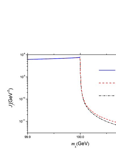
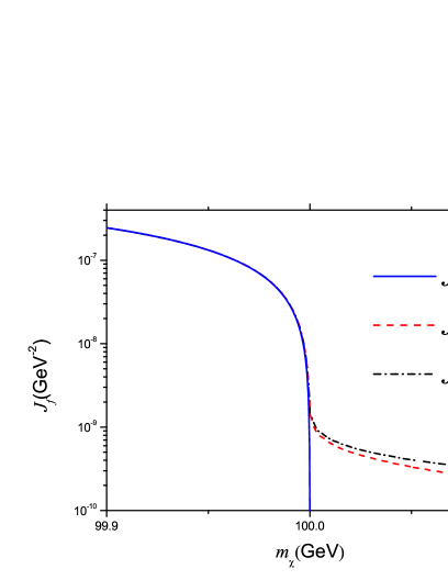
Figure 1: Analytical approximations $J_{f}^{d}$, $J_{f}^{a}$ and numerical result $J_{f}^{n}$ near the resonance point when $\chi$ is a scalar (a) or fermionic (b) DM particle in a specific case. The parameter values are taken as $\mu=1$ GeV, $\lambda_{f}=1$, $m_{R}$=200 GeV, $\sqrt{g_{*}}$=10, $x_{f}=20$, and $\Gamma_{R}=0.001$ GeV.

In Figure 1(b), we show the differences in approximate analytical results $J_{f}^{d}$, $J_{f}^{a}$, and the numerical result $J_{f}^{n}$ in a specific case where the parameters are taken as $\lambda_{f}=1$, $m_{R}$=200 GeV, $\sqrt{g_{*}}=10$, $x_{f}=20$, and $\Gamma_{R}=0.001$ GeV. As can be seen from the figure, if $m_{\chi}\lesssim 100$ GeV, the analytical result $J_{f}^{a}$ agrees with the numerical result $J_{f}^{n}$ well, the relative error is less than 5%, and the analytical $J_{f}^{d}$ can obtain the same precision if $\epsilon_{R}\gg\gamma_{R}$ is satisfied. If $m_{\chi}\gtrsim 100$ GeV, $J^{d}_{f}$ is no longer valid, but $J_{f}^{a}$ still agrees with $J_{f}^{n}$ near the resonance point well and the relative error is within 11% (in the region $100~{}{\rm~{}GeV}\lesssim m_{\chi}\lesssim 100.01$ GeV). On the resonance point, the relic density is given by

$$\Omega h^{2}\approx 2.755\times 10^{8}\sqrt{\frac{45}{\pi g_{*}}}\frac{8m_{\chi}^{2}}{\lambda_{f}^{2}M_{\rm Pl}\gamma_{R}\left[\ln(2x_{f}^{-1/2}\gamma_{R}^{-1})-4/\sqrt{\pi}\right]}{\rm GeV^{-1}}.$$ (27)

Unlike the $s$-wave case, the relic density is inversely proportional to $\gamma_{R}$.

If $\chi$ is Majorana fermion, we can write down the Lagrangian of $\chi$ interacting with $R$ as: $\mathcal{L}\supset\frac{1}{2}\lambda_{f}\overline{\chi}\chi R$, the expression for $\sigma v_{\rm rel}$ and relic density is identical to the case of Dirac DM.

3 DM direct detection

Direct detection experiments search for the signal of DM via their interactions with nucleus (for a review, see e.g.  [59]). A DM particle can interact with nuclei through $t$-channel scalar $R$ exchange. Since $R$ mixes with the Higgs boson, it can couple to the SM fermions with coupling constant $m_{f}/v_{s}$, where $m_{f}$ is the fermion mass and $v_{s}$ is a mass scale parameter. The decay width $\Gamma_{R}$ of the scalar $R$ is given by

$$\Gamma_{R}=\sum_{f}\frac{n_{c}\eta m_{f}^{2}}{8\pi v_{s}^{2}}\frac{(m_{R}^{2}-4m_{f}^{2})^{\frac{3}{2}}}{m_{R}^{2}},$$ (28)

where $n_{c}=3$(1) is the number of color for quarks (leptons), $\eta=1$(1/2) for (in)distinguishable final particles. If $\chi$ is a scalar DM particle, the spin-independent DM-nucleus elastic scattering cross section is given by[60]

$$\sigma_{n}^{\rm SI}=\frac{\mu_{\chi n}^{2}\mu^{2}}{4\pi m^{2}_{\chi}m^{4}_{R}}f_{n}^{2},$$ (29)

where $\mu_{\chi n}$ is the DM-nucleon reduced mass $\mu_{\chi n}=m_{\chi}m_{n}/(m_{\chi}+m_{n})$ with $m_{n}$ is the target nucleus mass. $f_{n}$ stands for the coupling between $R$ and nucleus, which is given by

$$\frac{f_{n}}{m_{n}}=\sum_{q=u,d,s}f^{(n)}_{Tq}\frac{a_{q}}{m_{q}}+\frac{2}{27}f^{(n)}_{TG}\sum_{q=c,b,t}\frac{a_{q}}{m_{q}},$$ (30)

where $f^{(n)}_{Tu}=0.011,\ f^{(n)}_{Td}=0.0273,$ and $f^{(n)}_{Ts}=0.0447$ [61]. The coupling $f^{(n)}_{TG}$ between DM and gluons from heavy quark loops is obtained from $f^{(n)}_{TG}=1-\Sigma_{q=u,d,s}f^{(n)}_{Tq}$, which leads to $f^{(n)}_{TG}=0.917$. In this case $a_{q}=m_{q}/v_{s}$, then

$$\sigma^{\rm SI}_{n}=\frac{0.02056\mu_{\chi n}^{2}m_{n}^{2}}{\pi v_{s}^{2}m_{R}^{4}m_{\chi}^{2}}\mu^{2}.$$ (31)

Making use of Eq. (27), (28), and the latest experimental observation $\Omega_{c}h^{2}=0.1199\pm 0.0027$ [62], we obtain the expression of $\sigma_{n}^{\rm SI}$ for the DM annihilation into SM fermions through the resonant state $R$

$$\sigma^{\rm SI}_{n}\approx\frac{4.12\times 10^{-12}\mu_{\chi n}^{2}m_{\chi}\gamma_{R}}{\sqrt{g_{*}}\sum\limits_{f}n_{c}\eta m_{f}^{2}(m_{\chi}^{2}-m_{f}^{2})^{\frac{3}{2}}}.$$ (32)

The above expression shows that $\sigma^{\rm SI}_{n}$ is proportional to $\gamma_{R}$.

For the fermionic DM particle described in section 2.2, it also interacts with nuclei through $t$-channel scalar $R$ exchange. The spin-independent DM-neucleus elastic scattering cross section is

$$\sigma^{\rm SI}_{n} = \frac{0.08224\mu_{\chi n}^{2}m_{n}^{2}}{\pi v_{s}^{2}m_{R}^{4}}\lambda_{f}^{2}$$ (33)

$$\approx \frac{1.65\times 10^{-11}\mu_{\chi n}^{2}m_{\chi}}{\sqrt{g_{*}}\left[\ln(2x_{f}^{-1/2}\gamma_{R}^{-1})-4/\sqrt{\pi}\right]\sum\limits_{f}n_{c}\eta m_{f}^{2}(m_{\chi}^{2}-m_{f}^{2})^{\frac{3}{2}}}.$$

Compared with the scalar DM case, $\sigma^{\rm SI}_{n}$ is not sensitive to $\gamma_{R}$.

For DM direct detection experiments, there is an irreducible background created by the coherent scattering of cosmic neutrinos off target neuclei. This irreducible background is very difficult to be distinguished from the interactions between DM-nuclei scattering, and it can set a limit on the sensitivity of DM direct detection experiments. Due to the neutrino background, the sensitivity of the spin-independent DM-nucleus scattering cross section $\sigma^{\rm SI}_{n}$ of DM direct detection experiments is limited to $10^{-46}~{}\rm cm^{2}\sim 10^{-48}~{}\rm cm^{2}$, depending on the DM mass[63, 64]. If $\sigma^{\rm SI}_{n}$ is below the neutrino background, the signal of DM particles can not be reached by DM direct detection experiments.

In Figure 2, we show the relation between $\sigma^{\rm SI}_{n}$ and $m_{\chi}$ on the resonance point with different values of $\gamma_{R}$ when $\chi$ is a scalar (a) or fermion (b). In Figure 2(a), for a typical DM particle mass $\sim 50$ GeV, $\sigma^{\rm SI}_{n}$ is above the neutrino background when the condition $\gamma_{R}\gtrsim 2.2\times 10^{-4}$ is satisfied. In Figure 2(b), $\sigma^{\rm SI}_{n}$ is always above the neutrino background, as long as the DM particle is lighter than the top quark.

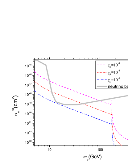
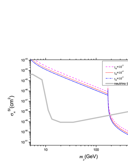
Figure 2: The relation between $\sigma_{n}^{\rm SI}$ and $m_{\chi}$ with different $\gamma_{R}$ for $\chi$ being a scalar (a) or fermion (b) DM particle. We take the parameters value $\sqrt{g_{*}}=10$, $x_{f}=20$.

4 Resonant annihilation in the real singlet dark matter model

In this section, we consider the resonant annihilation of DM particle in the real singlet DM model[17, 18, 19, 20, 21, 22, 23, 24, 25, 26]. The Lagrangian of the real singlet DM model is[17, 19]

$$\mathcal{L}=\mathcal{L}_{SM}+\frac{1}{2}\partial_{\mu}D\partial^{\mu}D-\frac{m_{0}^{2}}{2}D^{2}-\frac{\lambda_{D}}{4}D^{4}-\lambda_{H}D^{2}H^{\dagger}H,$$ (34)

where $\mathcal{L}_{SM}$ is the Lagrangian of SM, $H$ is the SM Higgs doublet. The linear and cubic terms are forbidden due to a discrete $Z_{2}$ symmetry $D\to-D$. $D$ has a vanishing vacuum expectation value (VEV) to ensure the DM stability. $\lambda_{D}$ describes the DM self-integration strength which is independent of the DM annihilation. It is clear that the DM-Higgs coupling $\lambda_{H}$ is the only one free parameter to regulate the DM annihilation. After the spontaneous symmetry breaking, one can obtain the DM mass $m_{D}^{2}=m_{0}^{2}+\lambda_{H}v_{0}^{2}$ with the vacuum expectation value $v_{0}=246$ GeV. In the real singlet dark matter model, the DM annihilation cross section is given by

$$\sigma v_{\rm rel}=\frac{8\lambda_{H}^{2}v_{0}^{2}}{(s-m_{H}^{2})^{2}+\Gamma_{H}^{2}m_{H}^{2}}\frac{\Gamma_{H}(\sqrt{s})}{2m_{D}},$$ (35)

where $\Gamma_{H}$ is the total decay width of Higgs which may decay to fermion pairs, gauge boson pairs and the real singlet DM pairs if $m_{H}>2m_{D}$[26], the value of $\Gamma_{H}(\sqrt{s})$ is given by

$$\Gamma_{H}(\sqrt{s}) = \frac{\sum n_{c}m_{f}^{2}}{8\pi v_{0}^{2}\eta}\frac{(s-4m_{f}^{2})^{1.5}}{s}+\frac{s^{\frac{3}{2}}}{32\pi v_{0}^{2}}\sqrt{1-\frac{4m_{Z}^{2}}{s}}\left(1-\frac{4m_{Z}^{2}}{s}+\frac{12m_{Z}^{4}}{s^{2}}\right)$$ (36)

$$+ \frac{s^{\frac{3}{2}}}{16\pi v_{0}^{2}}\sqrt{1-\frac{4m_{W}^{2}}{s}}\left(1-\frac{4m_{W}^{2}}{s}+\frac{12m_{W}^{4}}{s^{2}}\right)+\frac{\lambda^{2}v_{0}^{2}}{8\pi}\frac{\sqrt{s-4m_{D}^{2}}}{s}\;$$

and $\Gamma_{H}=\Gamma_{H}(\sqrt{s})|_{s=m^{2}_{H}}$. Eq. (35) can be written as

$$\sigma v_{\rm rel}=\frac{2\lambda_{H}^{2}v_{0}^{2}}{m_{D}^{4}}\frac{\gamma_{H}}{(v_{\rm rel}^{2}-\epsilon_{H})^{2}+\gamma_{H}^{2}},$$ (37)

where

$$\epsilon_{H}=\frac{m_{H}^{2}-4m_{D}^{2}}{m_{D}^{2}}\ {\rm and}\ \gamma_{H}=\frac{m_{h}\Gamma_{H}(m_{H})}{m_{D}^{2}}.$$ (38)

The real singlet DM model is a specific example for the case of $s$-wave annihilation we have discussed, the relic density for the real singlet DM and $\sigma_{n}^{\rm SI}$ near the resonance point is analogous with Eq. (2.1) and Eq. (31), and they can be obtained by substituting the parameters $\mu$, $\gamma_{R}$, and $\epsilon_{R}$ by 2$\lambda_{H}v_{0}$, $\gamma_{H}$, and $\epsilon_{H}$. Figure 3 shows the numerical and analytical value of $\sigma^{\rm SI}_{n}$, and the upper limits for the spin-independent DM-nucleus cross section from LUX[65] and XENON100[66]. In the figure, we find $\sigma^{\rm SI}_{n}$ is above the neutrino background and it is not excluded by the result of LUX and XENON100 near the resonance point ($m_{D}=m_{H}/2$).

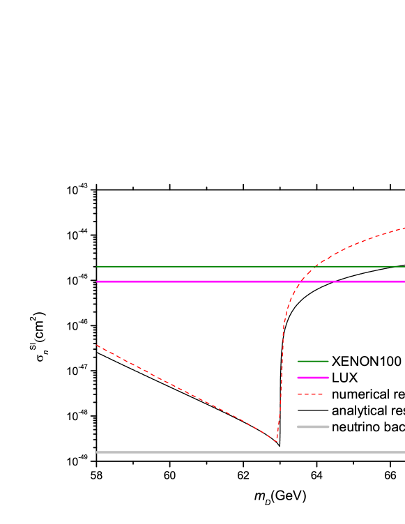
Figure 3: The value of $\sigma^{\rm SI}_{n}$ near the resonance point. Parameter values are $x_{f}=20$ and $\sqrt{{g_{*}}}=10$.

Currently the strongest upper limits on $\sigma^{\rm SI}_{n}$ are given by LUX experiment[65] and the next generation of DM direct detection experiments can push the upper bound on $\sigma^{\rm SI}_{n}$ down to $\sim\ 10^{-47}\ {\rm cm^{2}}$[67]. As the direct detection experiments at present can not measure the $\sigma^{\rm SI}_{n}$ below $10^{-46}\ {\rm cm^{2}}$, so we are uncertain of the existing of the real singlet DM near the resonance point. If the future direct detection experiments prove the region near the resonance is excluded, the real singlet DM will be removed from dark matter candidates. In conclusion, if we want to test the singlet dark matter model thoroughly by direct detection, the experiments’ ability should reach the minimum value of $\sigma^{\rm SI}_{n}$, which is about $2.6\times 10^{-49}\ {\rm cm^{2}}$.

5 Conclusion

In summary, we have presented an approximate analytical expression for the DM relic density of a scalar or fermionic DM particle which annihilates through an s-channel scalar resonance which has a narrow decay width. Based on the expression, we have investigated the condition for the DM-nuclei scattering cross section to be above the neutrino background. It is found that in Higgs-portal type models, for DM particles with $s$-wave annihilation, the spin-independent DM-nucleus scattering cross section is proportional to $\gamma_{R}$. For a typical DM particle mass $\sim 50$ GeV, the condition leads to $\gamma_{R}\gtrsim\mathcal{O}(10^{-4})$. In $p$-wave annihilation case, the spin-independent scattering cross section is insensitive to $\gamma_{R}$, and is always above the neutrino background, as long as the DM particle is lighter than the top quark. In the real singlet DM model, $\sigma^{\rm SI}_{n}$ is always above the neutrino background. In order to cover the full parameter space of this model, the required sensitivity should reach $\sim 2.6\times 10^{-49}~{}{\rm cm^{2}}$ for the next generation direct detection experiments.

References

- [1] Planck Collaboration, P. Ade et al., Planck 2013 results. I. Overview of products and scientific results, Astron.Astrophys. 571 (2014) A1, [arXiv:1303.5062].
- [2] PAMELA Collaboration, O. Adriani et al., An anomalous positron abundance in cosmic rays with energies 1.5-100 GeV, Nature 458 (2009) 607–609, [arXiv:0810.4995].
- [3] Fermi-LAT Collaboration, M. Ackermann et al., Measurement of separate cosmic-ray electron and positron spectra with the Fermi Large Area Telescope, Phys.Rev.Lett. 108 (2012) 011103, [arXiv:1109.0521].
- [4] AMS Collaboration, M. Aguilar et al., First Result from the Alpha Magnetic Spectrometer on the International Space Station: Precision Measurement of the Positron Fraction in Primary Cosmic Rays of 0.5 C350 GeV, Phys.Rev.Lett. 110 (2013) 141102.
- [5] AMS Collaboration, M. Aguilar et al., Electron and Positron Fluxes in Primary Cosmic Rays Measured with the Alpha Magnetic Spectrometer on the International Space Station, Phys.Rev.Lett. 113 (2014) 121102.
- [6] J. Hisano, S. Matsumoto, and M. M. Nojiri, Unitarity and higher order corrections in neutralino dark matter annihilation into two photons, Phys.Rev. D67 (2003) 075014, [hep-ph/0212022].
- [7] J. Hisano, S. Matsumoto, and M. M. Nojiri, Explosive dark matter annihilation, Phys.Rev.Lett. 92 (2004) 031303, [hep-ph/0307216].
- [8] J. Hisano, S. Matsumoto, M. M. Nojiri, and O. Saito, Non-perturbative effect on dark matter annihilation and gamma ray signature from galactic center, Phys.Rev. D71 (2005) 063528, [hep-ph/0412403].
- [9] N. Arkani-Hamed, D. P. Finkbeiner, T. R. Slatyer, and N. Weiner, A Theory of Dark Matter, Phys.Rev. D79 (2009) 015014, [arXiv:0810.0713].
- [10] Z.-P. Liu, Y.-L. Wu, and Y.-F. Zhou, Sommerfeld enhancements with vector, scalar and pseudoscalar force-carriers, Phys.Rev. D88 (2013) 096008, [arXiv:1305.5438].
- [11] J. Chen and Y.-F. Zhou, The 130 GeV gamma-ray line and Sommerfeld enhancements, JCAP 1304 (2013) 017, [arXiv:1301.5778].
- [12] Z.-P. Liu, Y.-L. Wu, and Y.-F. Zhou, Enhancement of dark matter relic density from the late time dark matter conversions, Eur.Phys.J. C71 (2011) 1749, [arXiv:1101.4148].
- [13] Z.-P. Liu, Y.-L. Wu, and Y.-F. Zhou, Dark Matter Conversion as a Source of Boost Factor for Explaining the Cosmic Ray Positron and Electron Excesses, J.Phys.Conf.Ser. 384 (2012) 012024, [arXiv:1112.4030].
- [14] A. De Simone, A. Riotto, and W. Xue, Interpretation of AMS-02 Results: Correlations among Dark Matter Signals, JCAP 1305 (2013) 003, [arXiv:1304.1336].
- [15] H.-B. Jin, Y.-L. Wu, and Y.-F. Zhou, Implications of the first AMS-02 measurement for dark matter annihilation and decay, JCAP 1311 (2013) 026, [arXiv:1304.1997].
- [16] H.-B. Jin, Y.-L. Wu, and Y.-F. Zhou, Cosmic ray propagation and dark matter in light of the latest AMS-02 data, arXiv:1410.0171.
- [17] V. Silveira and A. Zee, SCALAR PHANTOMS, Phys.Lett. B161 (1985) 136.
- [18] J. McDonald, Gauge singlet scalars as cold dark matter, Phys.Rev. D50 (1994) 3637–3649, [hep-ph/0702143].
- [19] C. Burgess, M. Pospelov, and T. ter Veldhuis, The Minimal model of nonbaryonic dark matter: A Singlet scalar, Nucl.Phys. B619 (2001) 709–728, [hep-ph/0011335].
- [20] H. Davoudiasl, R. Kitano, T. Li, and H. Murayama, The New minimal standard model, Phys.Lett. B609 (2005) 117–123, [hep-ph/0405097].
- [21] X.-G. He, T. Li, X.-Q. Li, J. Tandean, and H.-C. Tsai, The Simplest Dark-Matter Model, CDMS II Results, and Higgs Detection at LHC, Phys.Lett. B688 (2010) 332–336, [arXiv:0912.4722].
- [22] M. Gonderinger, Y. Li, H. Patel, and M. J. Ramsey-Musolf, Vacuum Stability, Perturbativity, and Scalar Singlet Dark Matter, JHEP 1001 (2010) 053, [arXiv:0910.3167].
- [23] Y. Mambrini, Higgs searches and singlet scalar dark matter: Combined constraints from XENON 100 and the LHC, Phys.Rev. D84 (2011) 115017, [arXiv:1108.0671].
- [24] J. M. Cline and K. Kainulainen, Electroweak baryogenesis and dark matter from a singlet Higgs, JCAP 1301 (2013) 012, [arXiv:1210.4196].
- [25] J. M. Cline, K. Kainulainen, P. Scott, and C. Weniger, Update on scalar singlet dark matter, Phys.Rev. D88 (2013) 055025, [arXiv:1306.4710].
- [26] W.-L. Guo and Y.-L. Wu, The Real singlet scalar dark matter model, JHEP 1010 (2010) 083, [arXiv:1006.2518].
- [27] Y.-L. Wu and Y.-F. Zhou, Two Higgs Bi-doublet Left-Right Model With Spontaneous P and CP Violation, Sci.China G51 (2008) 1808–1825, [arXiv:0709.0042].
- [28] Y.-L. Wu and Y.-F. Zhou, A Two Higgs Bi-doublet Left-Right Model With Spontaneous CP Violation, Int.J.Mod.Phys. A23 (2008) 3304–3308, [arXiv:0711.3891].
- [29] W.-L. Guo, L.-M. Wang, Y.-L. Wu, Y.-F. Zhou, and C. Zhuang, Gauge-singlet dark matter in a left-right symmetric model with spontaneous CP violation, Phys.Rev. D79 (2009) 055015, [arXiv:0811.2556].
- [30] W.-L. Guo, Y.-L. Wu, and Y.-F. Zhou, Exploration of decaying dark matter in a left-right symmetric model, Phys.Rev. D81 (2010) 075014, [arXiv:1001.0307].
- [31] W.-L. Guo, Y.-L. Wu, and Y.-F. Zhou, Searching for Dark Matter Signals in the Left-Right Symmetric Gauge Model with CP Symmetry, Phys.Rev. D82 (2010) 095004, [arXiv:1008.4479].
- [32] W.-L. Guo, Y.-L. Wu, and Y.-F. Zhou, Dark matter candidates in left-right symmetric models, Int.J.Mod.Phys. D20 (2011) 1389–1397.
- [33] J.-Y. Liu, L.-M. Wang, Y.-L. Wu, and Y.-F. Zhou, Two Higgs Bi-doublet Model With Spontaneous P and CP Violation and Decoupling Limit to Two Higgs Doublet Model, Phys.Rev. D86 (2012) 015007, [arXiv:1205.5676].
- [34] S.-S. Bao, H.-L. Li, Z.-G. Si, and Y.-F. Zhou, Probing and Interaction at LHC, Phys.Rev. D83 (2011) 115001, [arXiv:1103.1688].
- [35] Y. G. Kim and K. Y. Lee, The Minimal model of fermionic dark matter, Phys.Rev. D75 (2007) 115012, [hep-ph/0611069].
- [36] S. Baek, P. Ko, and W.-I. Park, Search for the Higgs portal to a singlet fermionic dark matter at the LHC, JHEP 1202 (2012) 047, [arXiv:1112.1847].
- [37] L. Lopez-Honorez, T. Schwetz, and J. Zupan, Higgs portal, fermionic dark matter, and a Standard Model like Higgs at 125 GeV, Phys.Lett. B716 (2012) 179–185, [arXiv:1203.2064].
- [38] S. Esch, M. Klasen, and C. E. Yaguna, Detection prospects of singlet fermionic dark matter, Phys.Rev. D88 (2013) 075017, [arXiv:1308.0951].
- [39] T. Li and Y.-F. Zhou, Strongly first order phase transition in the singlet fermionic dark matter model after LUX, JHEP 1407 (2014) 006, [arXiv:1402.3087].
- [40] S.-S. Bao, X. Gong, Z.-G. Si, and Y.-F. Zhou, Fourth generation Majorana neutrino, dark matter and Higgs physics, Int.J.Mod.Phys. A29 (2014) 1450010, [arXiv:1308.3021].
- [41] Y.-F. Zhou, Probing the fourth generation Majorana neutrino dark matter, Phys.Rev. D85 (2012) 053005, [arXiv:1110.2930].
- [42] J. R. Espinosa, T. Konstandin, and F. Riva, Strong Electroweak Phase Transitions in the Standard Model with a Singlet, Nucl.Phys. B854 (2012) 592–630, [arXiv:1107.5441].
- [43] D. J. Chung, A. J. Long, and L.-T. Wang, 125 GeV Higgs boson and electroweak phase transition model classes, Phys.Rev. D87 (2013), no. 2 023509, [arXiv:1209.1819].
- [44] J. Choi and R. Volkas, Real Higgs singlet and the electroweak phase transition in the Standard Model, Phys.Lett. B317 (1993) 385–391, [hep-ph/9308234].
- [45] S. Ham, Y. Jeong, and S. Oh, Electroweak phase transition in an extension of the standard model with a real Higgs singlet, J.Phys. G31 (2005) 857–872, [hep-ph/0411352].
- [46] A. Ahriche, What is the criterion for a strong first order electroweak phase transition in singlet models?, Phys.Rev. D75 (2007) 083522, [hep-ph/0701192].
- [47] S. Profumo, M. J. Ramsey-Musolf, and G. Shaughnessy, Singlet Higgs phenomenology and the electroweak phase transition, JHEP 0708 (2007) 010, [arXiv:0705.2425].
- [48] J. M. Cline, G. Laporte, H. Yamashita, and S. Kraml, Electroweak Phase Transition and LHC Signatures in the Singlet Majoron Model, JHEP 0907 (2009) 040, [arXiv:0905.2559].
- [49] J. R. Espinosa, B. Gripaios, T. Konstandin, and F. Riva, Electroweak Baryogenesis in Non-minimal Composite Higgs Models, JCAP 1201 (2012) 012, [arXiv:1110.2876].
- [50] M. Fairbairn and R. Hogan, Singlet Fermionic Dark Matter and the Electroweak Phase Transition, JHEP 1309 (2013) 022, [arXiv:1305.3452].
- [51] H.-B. Jin, S. Miao, and Y.-F. Zhou, Implications of the latest XENON100 and cosmic ray antiproton data for isospin violating dark matter, Phys.Rev. D87 (2013), no. 1 016012, [arXiv:1207.4408].
- [52] T. Li, S. Miao, and Y.-F. Zhou, Light mediators in dark matter direct detections, JCAP 1503 (2015), no. 03 032, [arXiv:1412.6220].
- [53] M. Ibe, H. Murayama, and T. Yanagida, Breit-Wigner Enhancement of Dark Matter Annihilation, Phys.Rev. D79 (2009) 095009, [arXiv:0812.0072].
- [54] W.-L. Guo and Y.-L. Wu, Enhancement of Dark Matter Annihilation via Breit-Wigner Resonance, Phys.Rev. D79 (2009) 055012, [arXiv:0901.1450].
- [55] G. Steigman, B. Dasgupta, and J. F. Beacom, Precise Relic WIMP Abundance and its Impact on Searches for Dark Matter Annihilation, Phys.Rev. D86 (2012) 023506, [arXiv:1204.3622].
- [56] K. Griest and D. Seckel, Three exceptions in the calculation of relic abundances, Phys.Rev. D43 (1991) 3191–3203.
- [57] P. Gondolo and G. Gelmini, Cosmic abundances of stable particles: Improved analysis, Nucl.Phys. B360 (1991) 145–179.
- [58] R. J. Scherrer and M. S. Turner, On the Relic, Cosmic Abundance of Stable Weakly Interacting Massive Particles, Phys.Rev. D33 (1986) 1585.
- [59] R. Gaitskell, Direct detection of dark matter, Ann.Rev.Nucl.Part.Sci. 54 (2004) 315–359.
- [60] A. Berlin, D. Hooper, and S. D. McDermott, Simplified Dark Matter Models for the Galactic Center Gamma-Ray Excess, Phys.Rev. D89 (2014), no. 11 115022, [arXiv:1404.0022].
- [61] G. Belanger, F. Boudjema, A. Pukhov, and A. Semenov, micrOMEGAs3: A program for calculating dark matter observables, Comput.Phys.Commun. 185 (2014) 960–985, [arXiv:1305.0237].
- [62] Planck Collaboration, P. Ade et al., Planck 2013 results. XVI. Cosmological parameters, Astron.Astrophys. 571 (2014) A16, [arXiv:1303.5076].
- [63] J. Billard, L. Strigari, and E. Figueroa-Feliciano, Implication of neutrino backgrounds on the reach of next generation dark matter direct detection experiments, Phys.Rev. D89 (2014), no. 2 023524, [arXiv:1307.5458].
- [64] A. Gutlein, C. Ciemniak, F. von Feilitzsch, N. Haag, M. Hofmann, et al., Solar and atmospheric neutrinos: Background sources for the direct dark matter search, Astropart.Phys. 34 (2010) 90–96, [arXiv:1003.5530].
- [65] LUX Collaboration, D. Akerib et al., First results from the LUX dark matter experiment at the Sanford Underground Research Facility, Phys.Rev.Lett. 112 (2014) 091303, [arXiv:1310.8214].
- [66] XENON100 Collaboration, E. Aprile et al., Dark Matter Results from 100 Live Days of XENON100 Data, Phys.Rev.Lett. 107 (2011) 131302, [arXiv:1104.2549].
- [67] XENON1T Collaboration, E. Aprile, The XENON1T Dark Matter Search Experiment, Springer Proc.Phys. C12-02-22 (2013) 93–96, [arXiv:1206.6288].