Supplementary Information for:

Spontaneous ordering of magnetic particles in liquid crystals: From chains to biaxial lamellae

Stavros D. Peroukidis and Sabine H.L. Klapp
Institute of theoretical Physics, Secr. EW 7-1, Technical University of Berlin, Hardenbergstr. 36, D-10623 Berlin, Germany

This supplementary information is organized in two sections: In Sec. I we present definitions for various pair distribution functions which we used to analyze our systems. Numerical results for rod-sphere mixtures with size ratios $\sigma_{\text{s}}^{*}=1$ and $\sigma_{\text{s}}^{*}=2$ are presented in Sec. II.

I Definitions of distribution functions

To analyze the positional ordering we consider various direction-dependent pair correlation functions in addition to the usual radial pair correlation functions $g^{({\text{a}})}\left(r\right)$ Veerman and Frenkel (1992); McGrother et al. (1996); Berardi and Zannoni (2000), where a= r (rods) or s (spheres). To start with, we calculate the longitudinal correlation function

$$g_{\|;\boldsymbol{\hat{n}}_{\text{a}}}^{\left({\text{a}}\right)}\left(r_{\|}\right)=\Big{\langle}\dfrac{\sum_{i\neq j}\delta\left(r_{\|}-\left|\boldsymbol{r}_{ij}\cdot\boldsymbol{\hat{n}}_{\text{a}}\right|\right)}{\Delta V_{2}\rho\left(N_{\text{a}}-1\right)}\Big{\rangle},$$ (1)

where $\Delta V_{2}=\pi\left(r^{2}-\left(\boldsymbol{r}_{ij}\cdot\boldsymbol{\hat{n}}_{\text{a}}\right)^{2}\right)\Delta r_{\|}$ is the volume of a cylindical shell with thickness $\Delta r_{\|}=0.05\sigma$. The function $g_{\|;\boldsymbol{\hat{n}}_{\text{a}}}^{\left({\text{a}}\right)}\left(r_{\|}\right)$ measures the distribution of particles of a specific type along the corresponding director, i.e., $r_{\|}$ is the projection of the connection vector $\boldsymbol{r}_{ij}$ onto $\boldsymbol{\hat{n}}_{\text{a}}$.

Likewise, the distribution perpendicular to the director of one species is measured by the correlation function

$$g_{\bot;\boldsymbol{\hat{n}}_{\text{a}}}^{\left({\text{a}}\right)}\left(r_{\bot}\right)=\Big{\langle}\dfrac{\sum_{i\neq j}\delta\left(r_{\bot}-\sqrt{r_{ij}^{2}-\left(\boldsymbol{r}_{ij}\cdot\boldsymbol{\hat{n}}_{\text{a}}\right)^{2}}\right)}{\Delta V_{3}\rho\left(N_{\text{a}}-1\right)}\Big{\rangle},$$ (2)

where $r_{\bot}=|\boldsymbol{r}_{ij}-\left(\boldsymbol{r}_{ij}\cdot\boldsymbol{\hat{n}}_{\text{a}}\right)\boldsymbol{\hat{n}}_{\text{a}}|$, and $\Delta V_{3}=\pi L\left(\left(r_{\bot}+\Delta r_{\bot}\right)^{2}-r_{\bot}^{2}\right)$ with $L$ being the height of the cylindrical shell.

Further, dipole-dipole correlations along the direction perpendicular to ${\hat{n}}_{\text{s}}$ are quantified by

$$g_{1;\boldsymbol{\hat{n}}_{\text{s}}}^{\left({\text{s}}\right)}\left(r_{\bot}\right)=\dfrac{\Big{\langle}\sum_{i\neq j}\delta\left(r_{\bot}-\sqrt{r_{ij}^{2}-\left(\boldsymbol{r}_{ij}\cdot\boldsymbol{\hat{n}}_{\text{s}}\right)^{2}}\right)\cos\theta_{ij}\Big{\rangle}}{\Big{\langle}\sum_{i\neq j}\delta\left(r_{\bot}-\sqrt{r_{ij}^{2}-\left(\boldsymbol{r}_{ij}\cdot\boldsymbol{\hat{n}}_{\text{s}}\right)^{2}}\right)\Big{\rangle}},$$ (3)

where $\cos\theta_{ij}=\boldsymbol{\hat{\mu}}_{i}\cdot\boldsymbol{\hat{\mu}}_{j}$, and $\boldsymbol{\hat{\mu}}_{i}$ is the dipolar unit vector of particle $i$.

Finally, to analyze the structure with respect to the dipole moment of one dipolar particle, we calculate the two-dimensional correlation function

$$g^{({\text{s}})}\left(r_{\|},r_{\bot}\right)=\Big{\langle}\dfrac{\sum_{i\neq j}\delta\left(r_{\bot}-\sqrt{r_{ij}^{2}-\left(\boldsymbol{r}_{ij}\cdot\boldsymbol{\hat{\mu}}_{i}\right)^{2}}\right)\delta\left(r_{\|}-\left|\boldsymbol{r}_{ij}\cdot\boldsymbol{\hat{\mu}}_{i}\right|\right)}{\Delta V\rho\left(N_{\text{s}}-1\right)}\Big{\rangle},$$ (4)

where $\Delta V=\pi\left(\left(r_{\bot}+\Delta r_{\bot}\right)^{2}-r_{\bot}^{2}\right)\Delta r_{\|}$.

II Numerical results for correlation functions

II.1 Mixtures with $\sigma^{*}_{\text{s}}=1.0$

We start by considering correlations between the rod particles. The structure formation of the rods with decreasing temperature at $\sigma_{\text{s}}^{*}=1.0$ (see Figs. 1 and 2 in the main manuscript) is indicated by the correlation function $g_{\|;\boldsymbol{\hat{n}}_{\text{r}}}^{\left({\text{r}}\right)}\left(r_{\|}\right)$ defined in Eq. (1). In Fig. 1 this function is plotted at density $\rho^{*}=0.4$ for two temperatures pertaining to the nematic and the smectic state, respectively.

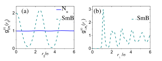
Figure 1: (Color online) (a) The correlation function $g_{\|;\boldsymbol{\hat{n}}_{\text{r}}}^{\left({\text{r}}\right)}\left(r_{\|}\right)$ and (b) $g_{\bot;\boldsymbol{\hat{n}}_{\text{r}}}^{\left({\text{r}}\right)}\left(r_{\bot}\right)$ in the uniaxial nematic (N${}_{\text{u}}$) state [$(T^{*},\rho^{*})=(1.2,0.40)$] and the smectic-B (SmB) state [$(T^{*},\rho^{*})=(0.9,0.40)$] at $\sigma^{*}_{\text{s}}=1.0$.

In the uniaxial nematic (N${}_{\text{u}}$) state, there are no appreciable correlations. This changes upon decreasing the temperature, where the undamped oscillations in $g_{\|;\boldsymbol{\hat{n}}_{\text{r}}}^{\left({\text{r}}\right)}\left(r_{\|}\right)$ clearly reflect the layering typical of a smectic state. The rod correlations $g_{\bot;\boldsymbol{\hat{n}}_{\text{r}}}^{\left({\text{r}}\right)}\left(r_{\bot}\right)$ perpendicular to $\boldsymbol{\hat{n}}_{\text{r}}$ [see Fig. 1(b)] indicate smectic-B (SmB) state characterized by local hexagonal ordering within the layers.

We now consider the dipolar particles. In the isotropic (I) state of the LC the dipolar spheres form a (globally isotropic) network of wormlike chains (see Fig. 2(a) of the main manuscript). A characteristic signature of this arrangement are the pronounced correlations along the dipole vector of a given particle. These are visible in Fig. 2 where we plot the two-dimensional pair correlation function defined in Eq. (4) at a representative I state.

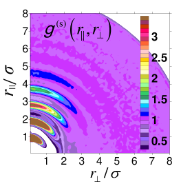
Figure 2: (Color online) Two-dimensional pair correlation function $g^{\left({\text{s}}\right)}\left(r_{\|},r_{\bot}\right)$ in the isotropic (I) state at $[(T^{*},\rho^{*})=(1.4,0.34)]$ and $\sigma_{\text{s}}^{*}=1.0$.

The correlations along the chains are reflected by the periodic arcs near the $r_{\|}$-axis. The lack of correlations along the $r_{\bot}$-axis indicate that neighboring chains are essentially decoupled, as expected due to the small density of DSS.

Finally, we present in Fig. 3 the influence of temperature on correlations between the dipolar spheres (for snapshots, see Fig. 2 in the main manuscript).

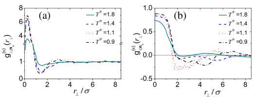
Figure 3: (Color online) The dipolar correlation functions (a) $g_{\bot;\boldsymbol{\hat{n}}_{\text{s}}}^{\left({\text{s}}\right)}\left(r_{\bot}\right)$ and (b) $g_{1;\boldsymbol{\hat{n}}_{\text{s}}}^{\left({\text{s}}\right)}\left(r_{\bot}\right)$ for $\rho^{*}=0.40$ and various temperatures $T^{*}$ ranging from the isotropic to the smectic-B regime ($\sigma^{*}_{\text{s}}=1.0$).

Figure 3(a) shows that for all temperatures considered, including the lowest ones corresponding to the uniaxial SmB state, the perpendicular distribution function $g_{\bot;\boldsymbol{\hat{n}}_{\text{s}}}^{\left({\text{s}}\right)}\left(r_{\bot}\right)$ takes large positive values only near the origin and then quickly decays to one (i.e., no correlations). Similarly, the dipole-dipole correlation function $g_{1;\boldsymbol{\hat{n}}_{\text{s}}}^{\left({\text{s}}\right)}\left(r_{\bot}\right)$, which is sensitive to the particle orientations, is positive (parallel orientation) only at very small distance in perpendicular direction. Both functions thus indicate that there are no polar domains beyond a single chain. Moreover, the polar chains lack of any long-range translational order.

II.2 Mixtures with $\sigma^{*}_{\text{s}}=2.0$

The mixtures with $\sigma^{*}_{\text{s}}=2.0$ are characterized by the appearance of a biaxial nematic (N${}_{\text{b}}$) and, at even lower temperature, a biaxial lamellar (L${}_{\text{b}}$) state (see Figs. 3 and 4 in the main manuscript). To understand the differences between these states on the level of correlation functions, we plot in Fig. 4 exemplary results for the rod-rod distribution function $g_{\|;\boldsymbol{\hat{n}}_{\text{r}}}^{\left({\text{r}}\right)}\left(r_{\|}\right)$ and the sphere-sphere distribution function $g_{\|;\boldsymbol{\hat{n}}_{\text{r}}}^{\left({\text{s}}\right)}\left(r_{\|}\right)$.

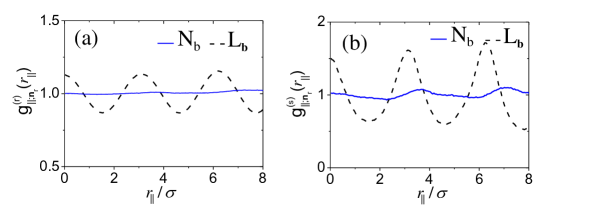
Figure 4: (Color online) The distribution functions (a) $g_{\|;\boldsymbol{\hat{n}}_{\text{r}}}^{\left({\text{r}}\right)}\left(r_{\|}\right)$ and (b) $g_{\|;\boldsymbol{\hat{n}}_{\text{r}}}^{\left({\text{s}}\right)}\left(r_{\|}\right)$ along the nematic director in the biaxial nematic (N${}_{\text{b}}$) state at $[(T^{*},\rho^{*})=(1.8,0.338)]$ and the biaxial lamellar (L${}_{\text{b}}$) state at $[(T^{*},\rho^{*})=(1.2,0.338)]$. The size ratio is $\sigma^{*}_{\text{s}}=2.0$. The data pertain to the system size $N=2536$.

At $T^{*}=1.8$ (N${}_{\text{b}}$ state), both distribution functions are essentially structureless, indicating that neither the rods nor the spheres are correlated along the nematic director. Upon further cooling into the L${}_{\text{b}}$ state, the function $g_{\|;\boldsymbol{\hat{n}}_{\text{r}}}^{\left({\text{r}}\right)}\left(r_{\|}\right)$ [see Fig. 4(a)] develops oscillations characteristic of the formation of a layered structure. Interestingly, this is also reflected by oscillations of the sphere distribution function $g_{\|;\boldsymbol{\hat{n}}_{\text{r}}}^{\left({\text{s}}\right)}\left(r_{\|}\right)$ along the rod $\boldsymbol{\hat{n}}_{\text{r}}$ director [see Fig. 4(b)]; these oscillations reflect the formation of dipolar layers between the rods (see Fig. 4(b) in the main manuscript). Indeed, the large peak at $r_{\|}\approx 3.13\sigma$ occurs at nearly the same value as that in $g_{\|;\boldsymbol{\hat{n}}_{\text{r}}}^{\left({\text{r}}\right)}\left(r_{\|}\right)$, reflecting that the length of the rods is the dominant length scale here.

Additional information about the distribution of spheres is gained by the function $g_{\bot;\boldsymbol{\hat{n}}_{\text{s}}}^{\left({\text{s}}\right)}\left(r_{\bot}\right)$ which is sensitive to structure formation perpendicular to the director characterizing the magnetic chains. Note that this function includes contributions from both, neighboring chains within a dipolar layer (see snapshot in Fig. 4(b)(inset) in the main manuscript) and neighboring chains in adjacent layers. A plot is shown in Fig. 5(b), while Fig. 5(a) contains for comparison the function $g_{\|;\boldsymbol{\hat{n}}_{\text{r}}}^{\left({\text{s}}\right)}\left(r_{\|}\right)$ [same data as in Fig. 4(b)].

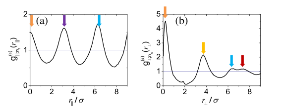
Figure 5: (Color online) The distribution functions (a) $g_{\|;\boldsymbol{\hat{n}}_{\text{r}}}^{\left({\text{s}}\right)}\left(r_{\|}\right)$ and (b) $g_{\bot;\boldsymbol{\hat{n}}_{\text{s}}}^{\left({\text{s}}\right)}\left(r_{\bot}\right)$ in the biaxial lamellar (L${}_{\text{b}}$) state [$(T^{*},\rho^{*})=(1.2,0.338)$, $\sigma^{*}_{\text{s}}=2.0$]. The maxima of the correlation function that are depicted by arrows correspond to distances in the sketch of the chain arrangement in Fig. 6.

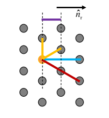
Figure 6: (Color online) Sketch of the (idealized) arrangement of magnetic chains inside the L${}_{\text{b}}$ state (for snapshots, see Fig. 4(b) main manuscript). The chains point randomly into or out of the plane. Also indicated is the director of the rods.

It is seen that $g_{\bot;\boldsymbol{\hat{n}}_{\text{s}}}^{\left({\text{s}}\right)}\left(r_{\bot}\right)$ [as does $g_{\|;\boldsymbol{\hat{n}}_{\text{r}}}^{\left({\text{s}}\right)}\left(r_{\|}\right)$] displays pronounced maxima indicative of the presence of short-ranged translational order of the ferromagnetic chains. Analyzing the positions of the maxima of both functions (indicated by colored arrows) we can draw a sketch of the arrangement of chains in the L${}_{\text{b}}$ state, see Fig. 6. Here, the chains point into (or out of) the plane, whereas the rod’s director lies horizontally. Thus, the chains are positioned within layers squeezed between the rods (see snapshot in Fig. 4(b) in the main manuscript). Of course, the sketch illustrates a highly idealized situation disregarding thermal fluctuations.

The spacing between the dipolar layers can be inferred from the positions of maxima in $g_{\|;\boldsymbol{\hat{n}}_{\text{r}}}^{\left({\text{s}}\right)}\left(r_{\|}\right)$ (see violet and light blue colors). The second peak of $g_{\bot;\boldsymbol{\hat{n}}_{\text{s}}}^{\left({\text{s}}\right)}\left(r_{\bot}\right)$ stems from chains in the adjacent layer, on the one hand, and from the two neighboring chains inside the layer, on the other hand. Interestingly, this peak (yellow) is positioned at a somewhat larger distance ($r_{\bot}\approx 3.7\sigma$) than that in the longitudinal function ($r_{\|}\approx 3.13\sigma$). Thus, the chains in adjacent layers are shifted, as indicated in Fig. 6. Finally, the light blue and red peaks in $g_{\bot;\boldsymbol{\hat{n}}_{\text{s}}}^{\left({\text{s}}\right)}\left(r_{\bot}\right)$ stem from correlations with chains the next nearest neighboring layer. Altogether, the correlations reflect that the chains are locally arranged into a rhombic-like structure.

References

- Veerman and Frenkel (1992) J. Veerman and D. Frenkel, Phys. Rev. A 45, 5632 (1992).
- McGrother et al. (1996) S. McGrother, D. Williamson, and G. Jackson, J. Chem. Phys. 104, 6755 (1996).
- Berardi and Zannoni (2000) R. Berardi and C. Zannoni, J. Chem. Phys. 113, 5971 (2000).