Deconfined criticality for the two-dimensional quantum -spin model with the three-spin and biquadratic interactions
Abstract
The criticality between the nematic and valence-bond-solid (VBS) phases was investigated for the two-dimensional quantum -spin model with the three-spin and biquadratic interactions by means of the numerical diagonalization method. It is expected that the criticality belongs to a novel universality class, the so-called deconfined criticality, accompanied with unconventional critical indices. In this paper, we incorporate the three-spin interaction, and adjust the (redundant) interaction parameter so as to optimize the finite-size behavior. Treating the finite-size cluster with spins, we estimate the correlation-length critical exponent as .
pacs:
75.10.Jm Quantized spin models and 05.30.-d Quantum statistical mechanics and 75.40.Mg Numerical simulation studies and 74.25.Ha Magnetic properties1 Introduction
The phase transition between the Néel and valence-bond-solid (VBS) phases for the two-dimensional quantum spin system is attracting much attention recently Senthil04 ; Senthil04b ; Levin04 ; Sandvik07 ; Melko08 ; Kuklov04 ; Kuklov08 ; Jian08 ; Kruger06 ; Chen13 ; Kotov09 ; Isaev10b ; Kaul11 ; Kaul12 ; Harada13 ; Pujari13 ; see Ref. Kaul13 for a review. It is expected that the phase transition, the so-called deconfined criticality, belongs to a novel universality class, accompanied with unconventional critical indices. Originally, the idea was developed Senthil04 ; Senthil04b ; Levin04 in the context of the gauge-field-theoretical description for the two-dimensional strongly-correlated-electron system. Meanwhile, it turned out that the underlying physics is common to a variety of systems in terms of the emergent gauge field Hikami79 ; Nogueira12 ; Wang14 ; Toldin14 .
As a lattice realization of the deconfined criticality, the quantum -spin square-lattice antiferromagnet with the plaquette four-spin interaction, the so-called - model Sandvik07 ; Melko08 , has been investigated extensively; the bipartite-lattice systems such as the square- Sandvik07 ; Melko08 and honeycomb-lattice Harada13 ; Pujari13 antiferromagnets do not conflict with the quantum Monte Carlo method, and large-scale-simulation results are available. However, it is still unclear whether the phase transition is critical Sandvik07 ; Melko08 ; Isaev10b ; Kaul11 ; Kaul12 ; Harada13 ; Pujari13 or a weak first-order transition with a latent-heat release Kuklov04 ; Kuklov08 ; Jian08 ; Kruger06 ; Chen13 ; Kotov09 . The controversy may be reconciled by a recent renormalization-group analysis Bartosch13 , which revealed an influence of a notorious marginal operator around the deconfined-critical fixed point; see Ref. Sandvik10 as well. Because the character of the marginal operator depends on each lattice realization, it may be sensible to survey a variety of lattice realizations.
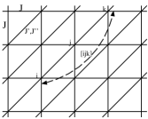
The -spin model is a clue to the realization of the deconfined criticality Harada07 ; Grover11 ; Nishiyama11 . A key ingredient is that the -spin model admits the biquadratic interaction, which stabilizes the VBS phase as the spatial anisotropy varies Fath95 . The phase transition separating the VBS and nematic Harada02 phases is expected to belong to the deconfined criticality Grover11 . We consider a non-bipartite-lattice version (Fig. 1); the details and underlying ideas are explained afterward. In the preceding paper Nishiyama11 , the correlation-length critical exponent was estimated as . In this paper, based on the preceding studies Harada07 ; Grover11 ; Nishiyama11 , we incorporate a rather novel interaction term intrinsic to the -spin model, namely, the three-spin-interaction term Michaud12 ; Wang13 (in addition to the biquadratic one), and survey the extended parameter space so as to optimize the finite-size behavior.
To be specific, we present the Hamiltonian for the two-dimensional -spin model
| (1) | |||||
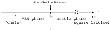
Here, the symbol denotes the quantum -spin operator placed at each square-lattice point (Fig. 1). The summations, , , and , run over all possible rectangular (nearest-neighbor) edges , skew-diagonal pairs , and skew-diagonal adjacent three sites , respectively. Correspondingly, the coupling constants, , , and , denote the nearest-neighbor-, skew-diagonal- and skew-diagonal-adjacent-three-spin-interaction parameters. Hereafter, the coupling constant is considered as the unit of energy (). The underlying physics behind each interaction parameter is as follows. For sufficiently large nearest-neighbor interaction , the system reduces to a two-dimensional model, and the nematic phase emerges Harada02 ; here, the quadratic component of the Heisenberg interaction is set to throughout this study. On the contrary, the coupling constants Fath95 and Michaud12 ; Wang13 strengthen the spatial anisotropy, promoting the formation of singlet dimers along the skew-diagonal bonds; a schematic phase diagram is presented in Fig. 2. In this paper, we incorporate the latter interaction term and adjust this (redundant) interaction parameter as well as the three-spin-interaction component so as to optimize the finite-size-scaling behavior.
It has to be mentioned that in the pioneering study Harada07 , the bipartite-lattice version (without the diagonal interaction) of Eq. (1) was investigated by means of the quantum Monte Carlo method; for the bipartite lattice, the spatial anisotropy inevitably violates the symmetry between the horizontal and vertical directions, and the asymmetry might alter the nature of the transition Harada13 . Our non-bipartite-lattice version (1) retains the symmetry (between the horizontal and vertical directions), as would be apparent from Fig. 1. In order to cope with the non-bipartite-type lattice, we employ the exact diagonalization method with the aid of Novotny’s method (screw-boundary condition) Novotny90 , which enables us to treat a variety of system sizes in a systematic manner; note that the number of spins constituting a rectangular cluster is restricted within .
The rest of this paper is organized as follows. In Sec. 2, we present the simulation results. The technical details as to the screw-boundary condition are presented as well. In Sec. 3, we address the summary and discussions, providing a brief overview on the past studies of the correlation-length critical exponent .
2 Numerical results
In this section, we present the simulation results. To begin with, we explain the simulation scheme to implement the screw-boundary condition, namely, Novotny’s method Novotny90 , briefly. Owing to this scheme, we are able to treat an arbitrary number of spins, , constituting a two-dimensional cluster. The linear dimension of the cluster is given by , because the spins form a rectangular cluster.
The Hamiltonian (1) has been investigated extensively in some limiting cases. In order to elucidate the phase diagram, Fig. 2, we recollect a number of related studies Fath95 ; Harada02 ; Michaud12 ; Wang13 ; we also address a brief account of the parameter range surveyed in our preliminary study. In the limit , the model reduces to the two-dimensional Heisenberg model with the biquadratic interaction. According to Ref. Harada02 , around , the nematic phase is realized. With and , the one-dimensional biquadratic-interaction Heisenberg model is realized, and the VBS phase emerges Fath95 . Similarly, with and , the VBS phase is realized for sufficiently large Michaud12 . Hence, the interaction parameter interpolates smoothly these limiting cases, and the phase diagram, Fig. 2, follows. In the preliminary stage of the research, we dwelt on the subspace , which was studied in Ref. Nishiyama11 . Turning on the interaction gradually, we arrive at the optimal regime , as indicated in Fig 5. At least for a moderate range of , a fundamental feature of the phase diagram, Fig. 2, is kept maintained; namely, no signature such as an appearance of a certain intermediate phase could be detected.
2.1 Simulation method: Screw-boundary condition
In this section, we explain Novotny’s method Novotny90 to implement the screw-boundary condition. The screw-boundary condition enables us to treat a variety of system sizes ; note that naively, the system size is restricted within quadratic numbers for a rectangular cluster.
In this paper, we follow the simulation scheme reported in Ref. Nishiyama11 , where the term of the Hamiltonian (1) was not taken into account. The missing term is incorporated by the addition of the following term to Eq. (5) of Ref. Nishiyama11 ;
| (2) |
(The index runs over a one-dimensional alignment in a way intrinsic to the screw-boundary condition.) Thereby, we diagonalize the Hamiltonian matrix given by Eq. (5) of Ref. Nishiyama11 with the term (2), employing the Lanczos algorithm for a finite-size cluster with spins. Rather technically, the diagonalization was performed within the zero-momentum subspace, at which the magnetic- (triplet-) excitation gap opens.
2.2 Finite-size scaling of : Critical point
In this section, based on the simulation method explained in Sec. 2.1, we evaluate the excitation gap . Thereby, we estimate the location of the critical point via the scaling analysis of .
In Fig. 3, we plot the scaled energy gap for various and (); here, the interaction parameters are set to and . According to the finite-size-scaling theory, the intersection point of indicates a location of the critical point , because the scaled energy gap should be scale-invariant (dimensionless) at the critical point.
In Fig. 4, we plot the approximate critical point for with (); the interaction parameters are the same as those of Fig. 3. Here, the approximate critical point is defined by the formula
| (3) |
for a pair of system sizes . The least-squares fit to the data in Fig. 4 yields in the thermodynamic limit . This extrapolated value does not affect the subsequent analysis (Sec. 2.3), and we do not go into the discussion of the extrapolation error; actually, the approximate critical point (rather than the extrapolated ) is fed into the formula, Eq. (4).
Last, we address a number of remarks. First, in Fig. 4, the finite-size behavior seems to be oscillatory; actually, the data exhibit successive bumps for quadratic values of . Such an oscillatory deviation is an artifact Novotny90 of the screw-boundary condition. Second, the set of the coupling constants and were determined so as to optimize the finite-size behavior of Fig. 4 (as well as Fig. 5 mentioned afterward). Actually, as for and , the finite-size behavior of suffers from steep finite-size drift and enhanced bumps. Last, in the scaling analysis, Fig. 3, we postulated the dynamical critical exponent . Here, we followed the conclusion obtained in the pioneering studies Sandvik07 ; Melko08 .
2.3 Correlation-length critical exponent
In this section, we estimate the correlation-length critical exponent . Based on the approximate critical point (3), we are able to calculate the approximate correlation-length critical exponent
| (4) |
for a pair of system sizes . In Fig. 5, as the symbol , we plot for with (); here, the interaction parameters are the same as those of Fig. 3. The data exhibit an oscillatory deviation (bump at ), which is an artifact of the screw-boundary condition Novotny90 . The least-squares fit to the data in Fig. 5 yields in the thermodynamic limit.
Similar analyses were carried out independently for various values of with fixed. As a consequence, the approximate critical point is plotted in Fig. 5 for () , () , and () . The least-squares fit to these data yields , , and , respectively, in the thermodynamic limit. Notably enough, the interaction parameter governs the convergence of to the thermodynamic limit. Particularly, in the optimal regime , the extrapolation to the thermodynamic limit can be taken reliability, allowing us to appreciate the critical exponent rather systematically. For exceedingly large , there emerge a notable finite-size drift (to the counter direction) as well as enhanced oscillatory deviations (steep bumps around ) as to and even , preventing us from extrapolating unambiguously. Surveying various as well as , we observed that the uncertainty of the extrapolation is bounded by . As a result, we estimate the correlation-length critical exponent as
| (5) |
The result is consistent with the estimate reported in Ref. Nishiyama11 , where the three-spin interaction was not taken into account.
In Fig. 5, we assumed implicitly that the dominant scaling correction should obey the power law . However, as mentioned in Introduction, there might be a logarithmic correction Bartosch13 ; Sandvik10 , which is not negligible for large system sizes. We cannot exclude a possibility that such a correction gives rise to an ambiguity as to the estimate (5). Here, aiming to provide a crosscheck, we carry out an alternative analysis of criticality as presented in the next section.
2.4 Scaling plot for
In this section, we present the scaling plot for as a cross-check of the analyses in Sec. 2.2 and 2.3.
In Fig. 6, we present the scaling plot, - for the same interaction parameters as those of Fig. 3. Here, the scaling parameters are set to (Sec. 2.2) and (Sec. 2.3). The scaled data appear to fall into a scaling curve satisfactorily for an appreciable range of , confirming the validity of the analyses in Sec. 2.2 and 2.3. As mentioned in Introduction, corrections-to-scaling behavior Bartosch13 ; Sandvik10 may depend on each lattice realization. In this respect, we stress that the present -spin model is less affected by severe scaling corrections.
This is a good position to address a remark on the validity of the deconfined-criticality scenario. As mentioned in Introduction, it is still unclear whether the (Néel-VBS) phase transition is continuous or not. The scaling analysis in Fig. 6 suggests that the (spatial-anisotropy-driven nematic-VBS) phase transition would be continuous. A notable point is that the estimate (5) takes a rather enhanced value; actually, it appears to be larger than, for instance, that of the Heisenberg universality class, Compostrini02 . Because of the following reason, such a feature might exclude a possibility of the discontinuous phase transition. As a matter of fact, the discontinuous phase transition does exhibit a pseudo-critical behavior (for finite system sizes) with an enhanced effective specific-heat critical exponent (: spatial dimension) Borgs90 . Resorting to the hyper-scaling relation , one arrives at a suppressed , which is inaccordant with ours. Such a tendency is reasonable, because the discontinuous transition is accompanied with a latent-heat release, enhancing the specific-heat critical exponent to a considerable extent. A comparison with other existing estimates for is presented in the next section.
3 Summary and discussions
The deconfined criticality between the nematic and VBS phases for the two-dimensional -spin model with both three-spin and biquadratic interactions (1) was investigated with the numerical diagonalization method for a finite-size cluster with spins; so far, the case without the three-spin interaction has been investigated extensively Harada07 ; Nishiyama11 . The extended interaction-parameter space enables us to search for a regime of suppressed finite-size corrections. Actually, the interaction parameter governs the convergence to the thermodynamic limit, as shown in Fig. 5. In fact, for , the extrapolation can be taken reliably. As a result, we estimate the correlation-length critical exponent as ; the result agrees with the preceeding estimate Nishiyama11 .
As a comparison, we recollect related studies of the deconfined criticality, placing an emphasis on the critical exponent . First, as mentioned in Introduction, the - model has been investigated extensively. Pioneering studies reported Sandvik07 and Melko08 . Possibly, there emerges the logarithmic corrections to scaling in the vicinity of the deconfined criticality Bartosch13 ; Sandvik10 , preventing us from identifying the character of the phase transition definitely. A recent simulation result for the honeycomb-lattice model indicated a rather suppressed value of Pujari13 . Second, a unique approach to the deconfined criticality was made by the extention of the internal symmetry to SU() with the continuously variable Beach09 . There was reported a clear evidence of the phase transition of a continuous character with the enhanced critical exponent -. Third, the “fermionic” criticality Hikami79 ; Nogueira12 indicates Wang14 and Toldin14 . Last, we overview simulation results for the classical counterparts. For the dimer model, the critical exponent was estimated as Charrier08 , Misguich08 , - Charrier10 , and - Papanikolaou10 . The hedgehog-suppressed O() model indicates an enhanced exponent Motruich04 . These conclusions have not been settled yet. Nonetheless, our result indicates a tendency toward an enhancement of such as the fermionic criticality Wang14 ; Toldin14 .
The present simulation result supports the deconfined-criticality scenario at least for the (spatial-anisotropy-driven) nematic-VBS phase transition; see the discussion in Sec. 2.4 as well. In Ref. Michaud13 , a novel two-dimensional quantum-spin model with the three-spin-interaction was introduced. The model may be a good clue to the realization of the deconfined criticality without the spatial anisotropy. However, its rich phase diagram has not been fully clarified. A progress toward this direction is remained for the future study.
Acknowledgment
This work was supported by a Grant-in-Aid for Scientific Research (C) from Japan Society for the Promotion of Science (Contact No. 25400402).


References
- (1) T. Senthil, A. Vishwanath, L. Balents, S. Sachdev, and M. P. A. Fisher, Science 303 (2001) 1490.
- (2) T. Senthil, L. Balents, S. Sachdev, A. Vishwanath, and M. P. A. Fisher, Phys. Rev. B 70 (2004) 144407.
- (3) M. Levin and T. Senthil, Phys. Rev. B 70 (2004) 220403.
- (4) A. W. Sandvik, Phys. Rev. Lett. 98 (2007) 227202.
- (5) R. G. Melko and R. K. Kaul, Phys. Rev. Lett. 100 (2008) 017203.
- (6) A. Kuklov, N. Prokof’ev, and B. Svistunov, Phys. Rev. Lett. 93 (2004) 230402.
- (7) A.B. Kuklov, M. Matsumoto, N.V. Prokof’ev, B.V. Svistunov, and M. Troyer, Phys. Rev. Lett. 101 (2008) 050405.
- (8) F.-J. Jiang, M. Nyfeler, S. Chandrasekharan, and U.-J. Wiese, J. Stat. Mech. (2008) P02009.
- (9) K. Krüger and S. Scheidl, Europhys. Lett. 74 (2006) 896.
- (10) Kun Chen, Yuan Huang, Youjin Deng, A. B. Kuklov, N. V. Prokof’ev, and B. V. Svistunov, Phys. Rev. Lett. 110 (2013) 185701.
- (11) V. N. Kotov, D.-X. Yao, A. H. Castro Neto, and D. K. Campbell, Phys. Rev. B 80 (2009) 174403.
- (12) L. Isaev, G. Ortiz, and J. Dukelsky, J. Phys.: Condens. Matter 22 (2010) 016006.
- (13) R. K. Kaul, Phys Rev B 84 (2011) 054407.
- (14) R. K. Kaul and A. W. Sandvik, Phys. Rev. Lett. 108 (2012) 137201.
- (15) K. Harada, T. Suzuki, T. Okubo, H. Matsuo, J. Lou, H. Watanabe, S. Todo, and N. Kawashima, Phys. Rev. B 88 (2013) 220408.
- (16) S. Pujari, K. Damle, and F. Alet, Phys. Rev. Lett. 111 (2013) 087203.
- (17) R. K. Kaul, R. G. Melko, and A. W. Sandvik, Annual Rev. Condens. Matter Phys. 4 (2013) 179.
- (18) S. Hikami, Prog. Theor. Phys. 62 (1979) 226.
- (19) F. Nogueira and A. Sudbø, Phys. Rev. B 86 (2012) 045121.
- (20) L. Wang. P. Corboz and M. Troyer, New J. Phys. 16 (2014) 103008.
- (21) F. P. Toldin, M. Hohenadler, F. F. Assaad and I. F. Herbut, arXiv: 1411.2502.
- (22) L. Bartosch, Phys. Rev. B 88 (2013) 195140.
- (23) A. W. Sandvik, Phys. Rev. Lett. 104 (2010) 177201.
- (24) K. Harada, N. Kawashima, and M. Troyer, J. Phys. Soc. Japan 76 (2007) 013703.
- (25) T. Grover and T. Senthil, Phys. Rev. Lett. 107 (2011) 077203.
- (26) Y. Nishiyama, Phys. Rev. B 83 (2011) 054417.
- (27) G. Fáth and J. Sólyom, Phys. Rev. B 51 (1995) 3620.
- (28) K. Harada and N. Kawashima, Phys. Rev. B 65 (2002) 052403.
- (29) F. Michaud, F. Vermay, S. R. Manmana and F. Mila, Phys. Rev. Lett. 108 (2012) 127202.
- (30) Z.-Y. Wang, S. C. Furuya, M. Nakamura and R. Komakura, Phys. Rev. B 88 (2013) 224419.
- (31) M.A. Novotny, J. Appl. Phys. 67 (1990) 5448.
- (32) M. Campostrini, M. Hasenbusch, A. Pelissetto, P. Rossi, and E. Vicari, Phys. Rev. B 65 (2002) 144520.
- (33) C. Borgs and R. Kotechký, J. Stat. Phys. 61 (1990) 79.
- (34) K. S. D. Beach, F. Alet, M. Mambrini, and S. Capponi, Phys. Rev. B 80 (2009) 184401.
- (35) D. Charrier, F. Alet and P. Pujol, Phys. Rev. Lett. 101 (2008) 167205.
- (36) G. Misguich, V. Pasquier, and F. Alet, Phys. Rev. B 78 (2008) 100402.
- (37) D. Charrier and F. Alet, Phys. Rev. B 82 (2010) 014429.
- (38) S. Papanikolaou and J.J. Betouras, Phys. Rev. Lett. 104 (2010) 045701.
- (39) O. I. Motrunich and A. Vishwanath, Phys. Rev. B 70 (2004) 075104.
- (40) F. Michaud and F. Mila, Phys. Rev. B 88 (2013) 094435.