Finite-time barriers to front propagation in two-dimensional fluid flows

Abstract

Recent theoretical and experimental investigations have demonstrated the role of certain invariant manifolds, termed burning invariant manifolds (BIMs), as one-way dynamical barriers to reaction fronts propagating within a flowing fluid. These barriers form one-dimensional curves in a two-dimensional fluid flow. In prior studies, the fluid velocity field was required to be either time-independent or time-periodic. In the present study, we develop an approach to identify prominent one-way barriers based only on fluid velocity data over a finite time interval, which may have arbitrary time-dependence. We call such a barrier a burning Lagrangian coherent structure (bLCS) in analogy to Lagrangian coherent structures (LCSs) commonly used in passive advection. Our approach is based on the variational formulation of LCSs using curves of stationary “Lagrangian shear”, introduced by Farazmand, Blazevski, and Haller [Physica D 278-279, 44 (2014)] in the context of passive advection. We numerically validate our technique by demonstrating that the bLCS closely tracks the BIM for a time-independent, double-vortex channel flow with an opposing “wind”.

Looking into a pocket near the edge of a lazy stream, one may see froth and small plant particulates twisting and evolving in sinuous strands. While streams are always subject to change—a branch falls in, a rock rolls, a fish swims nearby—the observed pattern changes little due to these differences in the stream’s current. An explanation for this is that the pattern organizes around a robust set of curves that form a “skeleton” for particulate advection.

While it is clear to the eye that such curves exist, it is another thing to define them precisely. A variety of techniques have been developed for this purpose, and while the original techniques were limited to flows that were either constant or periodic in time, the most general modern techniques can analyze flows with arbitrary time-dependence.

Considering now not a stream, but the entire ocean, one can find a teaming algae population within large eddies. The “living pattern” created by the swirling collection of replicating organisms is different from the passive particulates because the algae cluster is active—replication increases the size of the algae patch. There is a corresponding new set of “active” curves underlying the pattern formed by this growing front.

In this paper, we develop a technique to extract the most attracting and repelling curves for such active material within an arbitrary flow defined over a finite time interval. We imagine eventual application to improving management of oceanic algae blooms or to informing the design of combustion systems.

I Introduction

A growing interest has recently developed in fluid systems that combine the phenomenon of (chaotic) advection with that of front propagation. This interest is due in part to geophysical and technological applications, such as the growth of plankton blooms in oceanic flows Neufeld and Hernandez-Garcia (2009); Scotti and Pineda (2007); Sandulescu et al. (2008), the growth of the ozone hole in the atmosphere, and the spreading of chemical reactions in microfluidic devices. Another important driver of this field has been a steady accumulation of experimental observations and measurements of (Belousov-Zhabotinsky) chemical reaction fronts spreading in driven, laboratory-scale flows Paoletti and Solomon (2005, 2005); Paoletti et al. (2006); Schwartz and Solomon (2008); Boehmer and Solomon (2008); O’Malley et al. (2011); Pocheau and Harambat (2006, 2008); von Kameke et al. (2013), as well as early theoretical predictions on such advection-reaction-diffusion systems Abel et al. (2001, 2002); Cencini et al. (2003).

A recent advance in understanding advection-reaction-diffusion (ARD) systems is the realization that invariant manifold theory, familiar in the analysis of passive advective mixing MacKay et al. (1984); Ottino (1989); Rom-Kedar and Wiggins (1990); Wiggins (1992), is also applicable to the analysis of front propagation in fluids Mahoney et al. (2012); Mitchell and Mahoney (2012); Bargteil and Solomon (2012); Mahoney and Mitchell (2013); Mahoney et al. (2015); Gowen and Solomon (2014). Such manifolds have been called burning invariant manifolds, or BIMs, to distinguish them from their analogous, but distinct, advective counterparts. The most important property of BIMs is that they form time-invariant, or time-periodic, one-way barriers to front propagation in fluid flows that are themselves either time-invariant or time-periodic, respectively. The unstable BIMs are attracting structures, in that an initial stimulation near such a BIM ultimately creates a reaction front in the fluid that converges upon the BIM. In the most striking cases, this front persists for arbitrarily long times, forming a frozen or pinned front, whose profile follows the BIM Mahoney et al. (2015). Alternatively, stable BIMs are repelling structures. Initial stimulation points on either side have qualitatively distinct future behavior. Various other aspects of passive invariant manifolds extend to BIMs. For example, BIMs lead to a theory of turnstiles for front propagation in time-periodic fluid flows Mahoney and Mitchell (2013).

Despite the successful application of BIMs to ARD systems, their applicability has been limited to flows that are either time-independent or time-periodic. The present paper addresses this limitation by developing a theory of prominent, one-way barriers to front propagation in general fluid flows specified over a finite interval of time, with no assumption on the time-dependence over this interval. These barriers, called burning Lagrangian coherent structures (bLCSs), are either locally most repelling or most attracting. We validate this theory by numerically demonstrating that the bLCS reproduces the BIMs for time-independent flows considered over a sufficiently long time interval. A future publication will assess this theory in the general case of unsteady flows.

Our work is motivated by recent progress in the use of finite-time Lyapunov exponent (FTLE) fields Pierrehumbert and Yang (1993); von Hardenberg et al. (2000); Doerner et al. (1999); Haller (2001, 2002) and the associated Lagrangian coherent structures (LCSs) for passive advection in unsteady flows Haller (2000); Haller and Yuan (2000); Haller (2001, 2002, 2011); Shadden et al. (2005, 2006). A common approach in advection studies is to assume that ridges of the (forward) FTLE field are (repelling) LCSs that approximately separate trajectories with different future behavior. The FTLE ridge approach has its deficiencies, however, and can produce both false negatives and false positives when identifying LCSs Haller (2011), so it is best used, perhaps, as an intuitive diagnostic tool. That said, if one were to implement the FTLE-ridge approach for front-propagation dynamics, one would immediately encounter a challenge of dimensions. This is because the front-element dynamics in two spatial dimensions is naturally represented as a three-dimensional dynamical system, with $x$ and $y$ the two spatial coordinates and $\theta$ the orientation of the front element. (See Sect. II.) Note that the objects of our interest, the bLCSs, are still one-dimensional curves, just like the BIMs they seek to generalize; that is, a bLCS is not a codimension-one object in our study. Thus, a possible implementation of the FTLE-ridge approach to the front-element dynamics would not seek to follow 1D ridges in a 2D space, or even 2D ridges in a 3D space, but rather to follow 1D ridges in a 3D space. We see no obvious reason why such curves in the 3D phase space would correspond to fronts in the $xy$-position space, since a curve in the 3D space must satisfy the front-compatibility criterion (see Sect. II) for it to be the lift of a front in $xy$-space. It remains an open question, then, whether the 1D FTLE ridges would even yield fronts in the $xy$-position space, and assuming they did, these would undoubtedly suffer the same deficiencies noted in Ref. Haller (2011) for passive advection.

Instead of seeking FTLE ridges, we base our approach on the recent work of Farazmand, Blazevski, and Haller (FBH) Farazmand et al. (2014), which uses a variational principle to define the LCS. The advantage of a variational formulation is that it is based from the start on a search for curves in $xy$-space. These curves could be material lines, as in FBH Farazmand et al. (2014), or they could be fronts, as in the current study. The fact that the evolution of each front element depends on its orientation $\theta$ is naturally accommodated within the variational approach. Following FBH Farazmand et al. (2014), we base the variational integral on the Lagrangian shear, generalized to the front propagation dynamics. The output of the variational approach, when combined with the front compatibility criterion, is a flow on a 2D surface, which we call the shearless surface, embedded within the 3D phase space. This flow foliates the shearless surface into shearless fronts, which are candidates for a bLCS. This reduction to a 2D surface tames the challenge of dimensions discussed above. One can, for example, plot burning FTLE (bFTLE) fields on the 2D surface. However, the dimensional challenges have not been completely eliminated, since the shearless surface can have a complicated geometry within the 3D phase space, with folds and intersections that are not easily represented in a 2D projection. This geometry raises new considerations in the search for bLCSs that do not arise when searching for LCSs in passive advection.

This article has the following structure. Section II reviews our prior dynamical systems approach to front propagation in fluid flows and introduces the concept of BIMs as one-way barriers. Section III contains the core derivations. The main result is Theorem 39 of Sect. III.7, which identifies perfect shearless fronts as the candidates for a bLCS. Sect. III.8 describes how to compute these shearless fronts, and Sect. III.9 formulates the selection of the (repelling) bLCS from the set of shearless fronts as finding that front which maximizes the average normal repulsion. Section IV applies the bLCS approach to a time-independent double-vortex in a channel with wind. We study both short (Sect. IV.2) and long (Sect. IV.3) evolution times to show that the bLCS closely reproduces the BIM of the time-independent flow.

II Preliminaries

Following previous studies Mahoney et al. (2012); Mitchell and Mahoney (2012); Bargteil and Solomon (2012); Mahoney and Mitchell (2013); Mahoney et al. (2015); Gowen and Solomon (2014), we give a brief account of front propagation from the dynamical systems perspective. We make the sharp front assumption, in which the front marks a clear delineation between a reacted or “burned” region and an “unburned” region. Then, a front in a two-dimensional fluid flow can be represented as a curve $R(s)=(\mathbf{r}(s),\theta(s))$ in the three-dimensional $xy\theta$-space, where $s$ is an arbitrary smooth parameterization. Here $\theta$ denotes the orientation of the normal $\hat{\mathbf{n}}=(\sin\theta,-\cos\theta)$ and tangent $\hat{\mathbf{g}}=(\cos\theta,\sin\theta)$ to the front, where $\hat{\mathbf{n}}\times\hat{\mathbf{g}}=+1$. (Fig. 1.) The normal vector points in the propagation, or burning, direction of the front.

Figure 1: (color online) Each front element evolves according to Eqs. (2).

Not all curves in $xy\theta$-space represent fronts. There must be pointwise agreement between the tangent vector $\mathbf{r}^{\prime}=d\mathbf{r}/ds$ of the curve $\mathbf{r}(s)$ and the orientation $\hat{\mathbf{g}}(\theta)$ given by $\theta$. We call this the front-compatibility criterion

$$\frac{\mathbf{r}^{\prime}}{|\mathbf{r}^{\prime}|}=\pm\hat{\mathbf{g}}=\pm(\cos\theta,\sin\theta).$$ (1)

The front propagation speed $v_{0}$ in the local fluid frame, which we call the burning speed, is assumed to be isotropic and homogeneous throughout the fluid. Furthermore, we assume that $v_{0}$ is independent of the local curvature of the front or any other front property, i.e. $v_{0}$ is entirely constant in our analysis. Then each front element $(\mathbf{r},\theta)$ evolves independently of its neighboring front elements according to (see Fig. 1)

$$\frac{d\mathbf{r}}{dt} =\mathbf{u}+v_{0}\hat{\mathbf{n}},$$ (2a)

$$\frac{d\theta}{dt} =-\hat{n}_{i}u_{i,j}\hat{g}_{j},$$ (2b)

where $\mathbf{u}=\mathbf{u}(\mathbf{r},t)$ is the fluid velocity field, dot denotes the time derivative, comma denotes differentiation with respect to $r_{i}$, and repeated indices are summed. The fixed points of this dynamical system are called burning fixed points. For time-independent or time-periodic fluid velocity fields $\mathbf{u}(\mathbf{r},t)$, burning fixed points may have any combination of stable (S) and unstable (U) directions: SSS, SSU, SUU, UUU. The one-dimensional stable and unstable manifolds of SUU and SSU burning fixed points, respectively, play a special role and are called burning invariant manifolds (BIMs). BIMs satisfy the front-compatibility criterion and may thus be viewed as (virtual) fronts within the fluid. As such, they form one-way barriers to front propagation, owing to the fact that no front can catch up to and surpass another front moving in the same direction (what we call the no-passing lemma Mitchell and Mahoney (2012).) BIMs are thus natural, dynamically defined, geometric objects that restrict the propagation of fronts in an advecting fluid flow that is either time-independent or time-periodic.

III Coherent structures as solutions to an optimization problem

III.1 Lagrangian shear for fronts

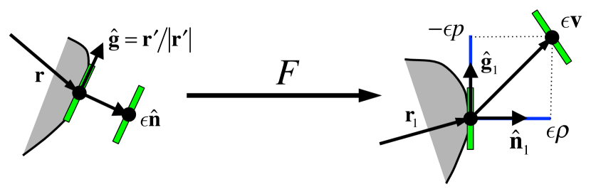
Figure 2: (color online) The definition of Lagrangian shear $p$ and normal repulsion $\rho$. An initial normal displacement $\epsilon\mathbf{\hat{n}}$ of a front element (left) evolves under $F$ into a displacement $\epsilon\mathbf{v}$ whose tangential projection (blue) is $-\epsilon$ times the Lagrangian shear $p$. The normal projection (blue) is $\epsilon$ times the normal repulsion.

We adapt the definition of Lagrangian shear in FBH Farazmand et al. (2014) to the front propagation scenario. We first assume that $\mathbf{u}(\mathbf{r},t)$ is given between an initial time $t_{0}$ and a final time $t_{1}=t_{0}+T$, with no requirement that the flow be time-independent or periodic. Then the evolution of a front element over this time interval is obtained by solving Eqs. (2). We denote the flow map acting on the 3D phase space by $F=F_{t_{0}}^{t_{1}}$. Consider now an initial front $R(s)=(\mathbf{r}(s),\theta(s))$ at time $t_{0}$, and suppose the element at a given position $\mathbf{r}(s)$ is displaced in the normal direction an infinitesimal distance $\epsilon\mathbf{\hat{n}}$. (The orientation $\theta$ of the front element is not perturbed.) Under the time evolution $F$, the point $R=(\mathbf{r},\theta)$ maps forward to $F(R)=R_{1}=(\mathbf{r}_{1},\theta_{1})$, and the relative displacement $\epsilon\hat{\mathbf{n}}$ between the original and perturbed front elements maps forward to a vector $\epsilon\mathbf{v}$ that will in general have a nonzero tangential projection onto the time-evolved front. (See Fig. 2.) We define the Lagrangian shear $p$ over the time interval $[t_{0},t_{1}]$ to be this projected length divided by $\epsilon$.

To compute $p$, we first note that the 3D normal displacement vector $[\hat{\mathbf{n}},0]$ at $t_{0}$ evolves forward to $\nabla F[\hat{\mathbf{n}},0]$ at $t_{1}$, where $\nabla F$ is the $3\times 3$ gradient of $F$, with components $(\nabla F)_{ij}=F_{i,j}$. Since $\mathbf{v}$, shown in Fig. 2, is the $xy$-component of $\nabla F[\hat{\mathbf{n}},0]$, we have

$$\mathbf{v}=\Pi_{xy}\nabla F\Pi_{xy}^{T}\hat{\mathbf{n}},$$ (3)

where

$$\Pi_{xy}=\left(\begin{array}[]{ccc}1&0&0\\ 0&1&0\end{array}\right)$$ (4)

is the restricted projection operator from the $xy\theta$-tangent space into the $xy$-tangent plane. Note $[\hat{\mathbf{n}},0]=\Pi_{xy}^{T}\hat{\mathbf{n}}$. We then define

$$[\nabla F]_{xy}=\Pi_{xy}\nabla F\Pi_{xy}^{T}$$ (5)

to be the $2\times 2$ restriction of $\nabla F$ to the $xy$-tangent plane. Note also that Eq. (1) implies

$$\hat{\mathbf{n}}=-\Omega\hat{\mathbf{g}}=\mp\Omega\mathbf{r}^{\prime}/|\mathbf{r}^{\prime}|,$$ (6)

where

$$\Omega=\left(\begin{array}[]{cc}0&-1\\ 1&0\\ \end{array}\right).$$ (7)

Then Eq. (3) becomes

$$\mathbf{v} =[\nabla F]_{xy}\hat{\mathbf{n}}$$ (8)

$$=\mp[\nabla F]_{xy}\Omega\mathbf{r}^{\prime}/|\mathbf{r}^{\prime}|.$$ (9)

We next need an expression for the tangent vector $\hat{\mathbf{g}}_{1}$ to the front at $\mathbf{r}_{1}$. The 3D tangent vector to the curve $R(s)$ at time $t_{0}$ is of the form $[\hat{\mathbf{g}},\alpha]$. This vector maps forward under $\nabla F$ to a vector whose $xy$-component $\Pi_{xy}\nabla F(\hat{\mathbf{g}},\alpha)$ is proportional to $\hat{\mathbf{g}}_{1}$. Note that this fact is actually true regardless of the value of $\alpha$, since $\alpha$ depends on the curvature $d\theta/ds$ of $\mathbf{r}(s)$ and not its tangent. We may thus set $\alpha=0$ to obtain

$$\hat{\mathbf{g}}_{1}=\frac{[\nabla F]_{xy}\hat{\mathbf{g}}}{|[\nabla F]_{xy}\hat{\mathbf{g}}|}=\pm\frac{[\nabla F]_{xy}\mathbf{r}^{\prime}}{|[\nabla F]_{xy}\mathbf{r}^{\prime}|},$$ (10)

where we again used the front-compatibility criterion Eq. (1). We are now in a position to compute $p$ via

$$p =\langle-\hat{\mathbf{g}}_{1},\mathbf{v}\rangle=\frac{\langle[\nabla F]_{xy}\mathbf{r}^{\prime},[\nabla F]_{xy}\Omega\mathbf{r}^{\prime}\rangle}{|\mathbf{r}^{\prime}||[\nabla F]_{xy}\mathbf{r}^{\prime}|}$$

$$=\frac{\langle\mathbf{r}^{\prime},[\nabla F]_{xy}^{T}[\nabla F]_{xy}\Omega\mathbf{r}^{\prime}\rangle}{\sqrt{\langle\mathbf{r}^{\prime},\mathbf{r}^{\prime}\rangle\langle\mathbf{r}^{\prime},[\nabla F]_{xy}^{T}[\nabla F]_{xy}\mathbf{r}^{\prime}\rangle}}.$$ (11)

The minus sign on $\hat{\mathbf{g}}_{1}$ conforms to the convention of FBH Farazmand et al. (2014). To summarize, we may express the Lagrangian shear as

$$p(\mathbf{r},\theta)=p(\mathbf{r},\mathbf{r}^{\prime}) =\frac{\langle\mathbf{r}^{\prime},C(\mathbf{r},\theta)\Omega\;\mathbf{r}^{\prime}\rangle}{\sqrt{\langle\mathbf{r}^{\prime},\mathbf{r}^{\prime}\rangle\langle\mathbf{r}^{\prime},C(\mathbf{r},\theta)\;\mathbf{r}^{\prime}\rangle}}$$ (12)

$$=\frac{\langle\mathbf{r}^{\prime},D(\mathbf{r},\theta)\;\mathbf{r}^{\prime}\rangle}{\sqrt{\langle\mathbf{r}^{\prime},\mathbf{r}^{\prime}\rangle\langle\mathbf{r}^{\prime},C(\mathbf{r},\theta)\;\mathbf{r}^{\prime}\rangle}},$$ (13)

where

$$C(\mathbf{r},\theta) =[\nabla F]_{xy}^{T}[\nabla F]_{xy},$$ (14)

$$D(\mathbf{r},\theta) =\frac{1}{2}(C(\mathbf{r},\theta)\Omega-\Omega C(\mathbf{r},\theta)).$$ (15)

Note that $C$ and $D$ are both $2\times 2$ symmetric matrices. We call $C$ the projected Cauchy-Green tensor. Note that even though $C$ is a $2\times 2$ matrix acting on the $xy$-tangent plane, it still depends on the orientation coordinate $\theta$. In the limit that the burning speed $v_{0}$ vanishes, the projected Cauchy-Green tensor reduces to the usual Cauchy-Green tensor defined for passive advection. Finally, note that we have written $p$ either as a function of $(\mathbf{r},\theta)$ or $(\mathbf{r},\mathbf{r}^{\prime})$, since $p$ does not depend on the magnitude of $\mathbf{r}^{\prime}$ and since $\theta$ is the angle of $\mathbf{r}^{\prime}$, as given by Eq. (1).

III.2 Normal repulsion for fronts

The bLCS will be defined to locally maximize the average normal repulsion $\rho$. Adapting the definition of normal repulsion in Ref. Haller (2011) to the front propagation scenario, we define $\rho$ to be the normal component of the time-evolved displacement $\mathbf{v}$ in Fig. 2. That is, the normal repulsion is a local measure of the degree to which a nearby front is pushed away, with $\rho>1$ indicating repulsion and $\rho<1$ attraction. To compute $\rho$, we shall need the normal $\hat{\mathbf{n}}_{1}$ at the final time $t_{1}$, which we claim is given by

$$\hat{\mathbf{n}}_{1}=\frac{[\nabla F]_{xy}^{-1T}\hat{\mathbf{n}}}{|[\nabla F]_{xy}^{-1T}\hat{\mathbf{n}}|}.$$ (16)

To prove this, we need only show that $\langle\hat{\mathbf{g}}_{1},\hat{\mathbf{n}}_{1}\rangle=0$. From Eqs. (10) and (16), $\langle\hat{\mathbf{g}}_{1},\hat{\mathbf{n}}_{1}\rangle$ is proportional to

$$\langle[\nabla F]_{xy}\mathbf{r}^{\prime},[\nabla F]_{xy}^{-1T}\hat{\mathbf{n}}\rangle =\langle[\nabla F]_{xy}^{-1}[\nabla F]_{xy}\mathbf{r}^{\prime},\hat{\mathbf{n}}\rangle$$

$$=\langle\mathbf{r}^{\prime},\hat{\mathbf{n}}\rangle=0.$$ (17)

Using Eq. (8), the normal repulsion is

$$\rho =\langle\hat{\mathbf{n}}_{1},\mathbf{v}\rangle=\frac{\langle[\nabla F]_{xy}^{-1T}\hat{\mathbf{n}},[\nabla F]_{xy}\hat{\mathbf{n}}\rangle}{|[\nabla F]_{xy}^{-1T}\hat{\mathbf{n}}|}$$

$$=\frac{1}{\sqrt{\langle[\nabla F]_{xy}^{-1T}\hat{\mathbf{n}},[\nabla F]_{xy}^{-1T}\hat{\mathbf{n}}\rangle}}=\frac{1}{\sqrt{\langle\hat{\mathbf{n}},C^{-1}\hat{\mathbf{n}}\rangle}}.$$ (18)

In summary, the normal repulsion is a function on the 3D phase space given by

$$\rho(\mathbf{r},\theta)=\rho(\mathbf{r},\mathbf{r}^{\prime})=\frac{1}{\sqrt{\hat{\mathbf{n}}\cdot C^{-1}(\mathbf{r},\theta)\hat{\mathbf{n}}}}.$$ (19)

III.3 Variational problem

The variational problem is now stated as follows. We seek a curve $\gamma$, parameterized as $\mathbf{r}(s)$, that makes the average Lagrangian shear

$$P[\gamma]=\frac{1}{\sigma}\int_{0}^{\sigma}p(\mathbf{r},\mathbf{r}^{\prime})ds$$ (20)

stationary under infinitesimal variations, where the average is taken over the interval $s_{0}\leq s\leq s_{0}+\sigma$, choosing the initial point to have parameter $s_{0}=0$. The endpoints of $\gamma$ are assumed fixed under the variations. Note that $p(\mathbf{r}(s),\mathbf{r}^{\prime}(s))$ does not depend on how the curve $\gamma$ is parameterized, since the numerator and denominator in Eq. (13) are both second order in $d/ds$. However, the average in Eq. (20) does depend on the parameterization through the line element $ds$. Different choices of the parameterization will change the weighting of the average along $\gamma$. The stationarity condition of $P[\gamma]$ should be understood not only in terms of variations in $\gamma$ but also in terms of variations of the parameterization $s$ along $\gamma$, with the interval of integration $[0,\sigma]$ held constant. (In contrast, one could use the euclidean line element $\sqrt{\langle\mathbf{r}^{\prime},\mathbf{r}^{\prime}\rangle}ds$ for the average, in which case $P[\gamma]$ would be independent of the parameterization of $\gamma$.) We shall find it useful to change the parameterization of the stationary curves, so we next summarize the reparameterization of trajectories in the Hamiltonian and Lagrangian formalisms.

III.4 Trajectory reparameterization for Hamiltonian systems

Suppose $(\mathbf{R}(s),\mathbf{P}(s))$ is a particular trajectory for an $s$-independent Hamiltonian $H(\mathbf{r},\mathbf{p})$ and let $E$ be the value of the (conserved) Hamiltonian along the trajectory. Here $s$ plays the role of time. Define a new trajectory parameterization $\tau$ by

$$d\tau/ds=\kappa(\mathbf{r},\mathbf{p}),$$ (21)

for some phase space function $\kappa$, and denote the reparameterized trajectory by $(\tilde{\mathbf{R}}(\tau),\tilde{\mathbf{P}}(\tau))$. Then $(\tilde{\mathbf{R}}(\tau),\tilde{\mathbf{P}}(\tau))$ is a trajectory of the Hamiltonian

$$\bar{H}_{E}(\mathbf{r},\mathbf{p})=\frac{1}{\kappa(\mathbf{r},\mathbf{p})}(H(\mathbf{r},\mathbf{p})-E),$$ (22)

where the (conserved) value of $\bar{H}_{E}$ along the trajectory is $\bar{E}=0$.

To prove this fact, we need only demonstrate $\dot{X}=\{X,\bar{H}_{E}\}$, where $X(\mathbf{r},\mathbf{p})$ is an arbitrary phase space quantity, $\{\;,\;\}$ denotes the Poisson bracket, and the dot denotes differentiation with respect to $\tau$. To this end,

$$\{X,\bar{H}_{E}\} =\{X,\kappa^{-1}(H-E)\}$$ (23)

$$=\{X,\kappa^{-1}\}(H-E)+\kappa^{-1}\{X,H-E\}$$ (24)

$$=\kappa^{-1}\{X,H\}=\kappa^{-1}X^{\prime}=\dot{X},$$ (25)

where the second to last equality utilizes

$$X^{\prime}=\{X,H\},$$ (26)

and the final equality uses Eq. (21).

III.5 Trajectory reparameterization for Lagrangian systems

Suppose $\mathbf{R}(s)$ is a particular trajectory for the $s$-independent Lagrangian $L(\mathbf{r},d\mathbf{r}/ds)$. We again let $E$ equal the value of the corresponding Hamiltonian along the trajectory. We also define a new parameterization $\tau$ by Eq. (21), except that $\kappa=\kappa(\mathbf{r},\mathbf{r}^{\prime})$ is expressed as a function of $\mathbf{r}^{\prime}$ rather than $\mathbf{p}$. Then the trajectory $\tilde{\mathbf{R}}(\tau)$, referred to the new parameterization, is a trajectory of the Lagrangian

$$\bar{L}_{E}(\mathbf{r},\dot{\mathbf{r}})=\frac{1}{\tilde{\kappa}(\mathbf{r},\dot{\mathbf{r}})}(\tilde{L}(\mathbf{r},\dot{\mathbf{r}})+E),$$ (27)

where $\tilde{L}$ and $\tilde{\kappa}$ are $L$ and $\kappa$ re-expressed as functions of

$$\dot{\mathbf{r}}=\frac{1}{\kappa}\mathbf{r}^{\prime}.$$ (28)

To prove this, we recall the Legendre transforms

$$H =\langle\mathbf{p},\mathbf{r}^{\prime}\rangle-L,$$ (29)

$$\bar{H}_{E} =\langle\mathbf{p},\dot{\mathbf{r}}\rangle-\bar{L}_{E},$$ (30)

where the momentum $\mathbf{p}$ is

$$\mathbf{p}=\partial L/\partial\mathbf{r}^{\prime}=\partial\bar{L}_{E}/\partial\dot{\mathbf{r}}.$$ (31)

Substituting Eqs. (29) and (30) into Eq. (22) yields Eq. (27).

III.6 Reparameterizing stationary curves of the average Lagrangian shear

Defining the Lagrangian $L=p$, Eq. (13) yields

$$L(\mathbf{r},\mathbf{r}^{\prime})=\frac{\langle\mathbf{r}^{\prime},D(\mathbf{r},\theta)\;\mathbf{r}^{\prime}\rangle}{\sqrt{\langle\mathbf{r}^{\prime},\mathbf{r}^{\prime}\rangle\langle\mathbf{r}^{\prime},C(\mathbf{r},\theta)\;\mathbf{r}^{\prime}\rangle}}.$$ (32)

Re-expressing this in terms of the transformed derivative $\dot{\mathbf{r}}$, Eq. (28), yields

$$\tilde{L}(\mathbf{r},\dot{\mathbf{r}})=\frac{\langle\dot{\mathbf{r}},D\;\dot{\mathbf{r}}\rangle}{\sqrt{\langle\dot{\mathbf{r}},\dot{\mathbf{r}}\rangle\langle\dot{\mathbf{r}},C\;\dot{\mathbf{r}}\rangle}},$$ (33)

which has the same functional form as Eq. (32), since the $\mathbf{r}$ derivative occurs at the same order (two) in both the numerator and denominator. We now choose

$$\tilde{\kappa}(\mathbf{r},\dot{\mathbf{r}})=\frac{1}{\sqrt{\langle\dot{\mathbf{r}},\dot{\mathbf{r}}\rangle\langle\dot{\mathbf{r}},C\;\dot{\mathbf{r}}\rangle}},$$ (34)

so that Eq. (27) becomes

$$\bar{L}_{E}(\mathbf{r},\dot{\mathbf{r}})=\langle\dot{\mathbf{r}},D\;\dot{\mathbf{r}}\rangle+E\sqrt{\langle\dot{\mathbf{r}},\dot{\mathbf{r}}\rangle\langle\dot{\mathbf{r}},C\;\dot{\mathbf{r}}\rangle}.$$ (35)

Equation (31) implies $\langle\mathbf{p},\mathbf{r}^{\prime}\rangle=\langle\mathbf{r}^{\prime},\partial L/\partial\mathbf{r}^{\prime}\rangle$, which is just the derivative of $L$ in the direction of increasing radius $|\mathbf{r}^{\prime}|$ in the $\mathbf{r}^{\prime}$-space. Investigating Eq. (32), however, we see that the dependence of $L$ on $\mathbf{r}^{\prime}$ is solely through the angle $\theta$ of $\mathbf{r}^{\prime}$ and not $|\mathbf{r}^{\prime}|$. Thus, $\langle\mathbf{p},\mathbf{r}^{\prime}\rangle=0$. Furthermore, since $\mathbf{r}^{\prime}=\kappa\dot{\mathbf{r}}$, $\langle\mathbf{p},\dot{\mathbf{r}}\rangle=0$ as well. Thus, Eqs. (29) and (30) imply

$$H=L,\quad\quad\bar{H}_{E}=\bar{L}_{E}.$$ (36)

Since $\bar{E}=0$, the value of $\bar{L}_{E}$ along the stationary trajectory $\mathbf{R}(\tau)$ also vanishes. These results were obtained by FBH Farazmand et al. (2014) through an alternative derivation.

Theorem 1

Every stationary curve $\gamma$ of the average Lagrangian shear $P[\gamma]$, Eq. (20), is also a stationary curve of

$$\bar{P}_{E}[\gamma] =\frac{1}{\tau_{f}}\int_{0}^{\tau_{f}}\bar{L}_{E}(\mathbf{r},\dot{\mathbf{r}})d\tau$$ (37)

$$=\frac{1}{\tau_{f}}\int_{0}^{\tau_{f}}\left(\langle\dot{\mathbf{r}},D\;\dot{\mathbf{r}}\rangle+E\sqrt{\langle\dot{\mathbf{r}},\dot{\mathbf{r}}\rangle\langle\dot{\mathbf{r}},C\;\dot{\mathbf{r}}\rangle}\right)d\tau,$$ (38)

where $E$ is the (conserved) value of the Lagrangian shear $p$ along $\gamma$. The value of $\bar{L}_{E}$ along $\gamma$ is also conserved and equal to 0. Note that the parameterization $\bar{\mathbf{R}}(\tau)$ of $\gamma$ that makes $\bar{P}_{E}$ stationary is typically different from the parameterization $\mathbf{R}(s)$ of $\gamma$ that makes $P$ stationary.

III.7 Perfect shearless fronts

Equations (32) and (36) show that $E=0$ is equivalent to $\langle\dot{\mathbf{r}},D\dot{\mathbf{r}}\rangle=0$. Furthermore, one can show that any curve satisfying $\langle\dot{\mathbf{r}},D\dot{\mathbf{r}}\rangle=0$ is a stationary curve of Eq. (38). Thus, we have the following.

Theorem 2

A curve $\gamma$ satisfying $\langle\dot{\mathbf{r}},D\;\dot{\mathbf{r}}\rangle=0$, or equivalently $p=0$, is a stationary curve of

$$\bar{P}_{0}[\gamma]=\frac{1}{T}\int_{0}^{T}\langle\dot{\mathbf{r}},D\;\dot{\mathbf{r}}\rangle d\tau.$$ (39)

We call such curves perfect shearless fronts (analogous to the perfect shearless barriers of FBH Farazmand et al. (2014)), or just shearless fronts for short. They are the focus of the remainder of this article.

Note that since $D$ is symmetric and traceless [see Eq. (15)], it is like a pseudo-Riemannian metric tensor; “pseudo” because it has signature $(-1,1)$. However, the resulting metric fails to be given purely by a bilinear form, since $D$ itself depends on $\theta$. Such a metric is called a (pseudo-)Finsler metric. Perfect shearless fronts are thus light-like, or null, geodesics of this pseudo-Finsler metric.

III.8 Computing perfect shearless fronts

In Sects. III.3, III.6, and III.7, fronts were viewed as curves in the $xy$-position space for the purpose of the variational problem. Referring now to the full $xy\theta$-phase space, a shearless front $(\mathbf{r}(\tau),\theta(\tau))$ satisfies both the front compatibility criterion Eq. (1) and $\langle\dot{\mathbf{r}},D\dot{\mathbf{r}}\rangle=0$. The latter implies that $\langle\dot{\mathbf{r}},C\Omega\dot{\mathbf{r}}\rangle=0$, and hence that $\dot{\mathbf{r}}$ is an eigenvector of $C(\mathbf{r},\theta)$. One possible approach to finding the shearless fronts, then, is to integrate an eigenvector field of $C(\mathbf{r},\theta)$. Let $\hat{\xi}(\mathbf{r},\theta)$ denote a choice of unit eigenvector over $xy\theta$-space. Taking $\dot{\mathbf{r}}$ proportional to $\hat{\xi}$, the front compatibility criterion Eq. (1) becomes

$$\chi(\mathbf{r},\theta)=0,$$ (40)

where

$$\chi(\mathbf{r},\theta)=\mathbf{\hat{n}}(\theta)\cdot\hat{\mathbf{\xi}}(\mathbf{r},\theta)=(\sin\theta\mathbf{\hat{x}}-\cos\theta\mathbf{\hat{y}})\cdot\hat{\mathbf{\xi}}(\mathbf{r},\theta).$$ (41)

This quantity is zero at $(\mathbf{r},\theta)$ if and only if $\mathbf{\hat{g}}(\theta)=\pm\hat{\mathbf{\xi}}(\mathbf{r},\theta)$. If the choice of $\hat{\xi}(\mathbf{r},\theta)$ were smooth everywhere, then Eq. (40) would define a smooth two-dimensional constraint manifold in $xy\theta$-space. In general, however, there is no continuous choice of $\hat{\xi}(\mathbf{r},\theta)$ available over the entire phase space. The continuity of $\hat{\xi}(\mathbf{r},\theta)$ can break down at points in $xy\theta$-space where $C(\mathbf{r},\theta)$ has degenerate eigenvalues, and hence where there is not a unique eigendirection. Since degeneracy of real symmetric two-by-two matrices is a codimension-two criterion, the degeneracy points generically occur along curves in $\mathbf{r}\theta$-space. Even if we remove these degenerate curves from consideration, $\hat{\xi}(\mathbf{r},\theta)$ can not in general be chosen continuously on the remainder of $xy\theta$-space. This is due to the fact that $\hat{\xi}(\mathbf{r},\theta)$ may obtain an overall rotation by $\pi/2$ when transported along a loop encircling a degenerate curve.

Rather than finding the eigenvectors explicitly, an improved approach is to use the constraint equation

$$\psi(\mathbf{r},\theta)=0,$$ (42)

where

$$\psi(\mathbf{r},\theta) =\mathbf{\hat{n}}(\theta)\cdot C(\mathbf{r},\theta)\mathbf{\hat{g}}(\theta)$$ (43)

$$=(\sin\theta\mathbf{\hat{x}}-\cos\theta\mathbf{\hat{y}})\cdot C(\mathbf{r},\theta)(\cos\theta\mathbf{\hat{x}}+\sin\theta\mathbf{\hat{y}}).$$ (44)

This quantity is zero at $(\mathbf{r},\theta)$ if and only if $\mathbf{\hat{g}}(\theta)$ is any eigenvector of $C(\mathbf{r},\theta)$, not just a particular choice $\hat{\xi}(\mathbf{r},\theta)$ as above. The constraint surface Eq. (42) can thus be understood as the union of the two surfaces defined by Eq. (40) for the two choices of eigenvector $\hat{\mathbf{\xi}}$. The constraint surface Eq. (42) is a smooth surface without boundary (though potentially with self-intersections), which we call the shearless surface.

A perfect shearless front, lifted into $xy\theta$-space via the front compatibility condition, must lie within the shearless surface. A perfect shearless front is thus an integral curve of a vector field tangent to the shearless surface. This vector field, normalized to unity, is

$$\frac{d\mathbf{r}}{d\lambda} =\frac{a}{\sqrt{a^{2}+b^{2}}}\mathbf{\hat{g}},$$ (45)

$$\frac{d\theta}{d\lambda} =\frac{b}{\sqrt{a^{2}+b^{2}}},$$

where

$$a =-\frac{d}{d\theta}\psi,$$ (46)

$$b =\mathbf{\hat{g}}\cdot{\bm{\nabla}}\psi.$$

An integral curve of (45) will lie within the shearless surface so long as its initial condition does. Note that these vector fields do not require us to find the eigenvectors of $C(\mathbf{r},\theta)$.

We shall also need the vector field that is everywhere orthogonal to Eq. (45), but still tangent to the shearless surface. This field is obtained by replacing $\hat{\mathbf{g}}$ by $\hat{\mathbf{n}}$ in Eqs. (45) and (46), i.e.,

$$\frac{d\mathbf{r}}{d\kappa} =\frac{a}{\sqrt{a^{2}+c^{2}}}\mathbf{\hat{n}},$$ (47)

$$\frac{d\theta}{d\kappa} =\frac{c}{\sqrt{a^{2}+c^{2}}},$$

where $\kappa$ parameterizes the curve and

$$a =-\frac{d}{d\theta}\psi,$$ (48)

$$c =\mathbf{\hat{n}}\cdot{\bm{\nabla}}\psi.$$

III.9 Burning Lagrangian coherent structures (bLCSs) as shearless fronts of maximal normal repulsion

The normal repulsion $\rho$ of a front element $(\mathbf{r},\theta)$ is given by Eq. (19). On the shearless surface, where $\hat{\mathbf{n}}$ is an eigenvector of $C$, this simplifies to

$$\rho(\mathbf{r},\theta) =\sqrt{\hat{\mathbf{n}}\cdot C(\mathbf{r},\theta)\hat{\mathbf{n}}}=\sqrt{\lambda_{\perp}},$$ (49)

where $\lambda_{\perp}$ is the eigenvalue of $C$ normal to the tangent. We now define the burning finite-time Lyapunov exponent (bFTLE) field as

$$\Lambda=\frac{1}{2T}\log(\lambda_{\perp})=\frac{1}{T}\log(\rho).$$ (50)

Note that the specification of the eigenvalue $\lambda_{\perp}$ is based on the orientation of its eigenvector (normal to the front) rather than its magnitude; thus $\lambda_{\perp}$ need not be the largest eigenvalue.

Since the bFTLE is defined on the two-dimensional shearless surface, we have overcome part of the challenge of dimensions highlighted in Sect. I. In particular, we can plot and visually interpret images of the bFTLE (Fig. 4a). In some cases a bLCS follows a ridge of the bFTLE field. However, we see no reason why a ridge of the bFTLE field need satisfy the front-compatibility criterion, and so we opt not to compute bFTLE ridges. Again, we see the advantage of using the shearless fronts, for which the problem of defining the bLCS becomes the problem of selecting the “best” curve from the one-parameter family of shearless fronts. We choose the repelling bLCS to be that shearless front that (locally) maximizes the average normal repulsion

$$R[\gamma]=\frac{1}{L}\int_{\gamma}\sqrt{\hat{\mathbf{n}}\cdot C(\mathbf{r},\theta)\hat{\mathbf{n}}}\;d\ell,$$ (51)

where $d\ell$ is the $xy$-euclidean line element and $L$ is the euclidean length of the curve. Similarly, the attracting bLCS is that shearless front that (locally) minimizes the average normal repulsion.

There is still a question of what interval length $L$ to choose. In keeping with the intuitive idea of following an bFTLE ridge, we shall adopt the approach of Refs. Haller (2011); Farazmand and Haller (2012) and restrict the length of a shearless front to those regions of the shearless surface where the second derivative of the bFTLE field in the direction normal to the front, given by Eqs. (47), is negative. In practice, the exact length used should make little difference, so we use the curvature criterion to tell us approximately where to cut the shearless curves.

III.10 Cusps in the shearless fronts

The shearless fronts, and hence a bLCS, may exhibit cusps when plotted in $xy$-space. This is one consequence of the 3D phase-space geometry that does not occur for traditional LCSs in passive advection. Cusps have already been recognized as important features of BIMs for time-independent and time-periodic flows (see Fig. 3a); cusps change the one-way barrier direction of the BIMs. Here, we determine when a cusp occurs along a shearless front. First, we consider the fold of the shearless surface under the projection from the $xy\theta$-space to the $xy$-space; a fold is where two branches of this projection meet. Since a shearless front is smooth on the shearless surface, if it remains on one branch of this surface, then its projection to $xy$-space is also smooth. Thus, a cusp of a shearless front can only occur at a fold of the shearless surface. What is less obvious, but nevertheless true, is that every time a shearless front passes around a fold, its $xy$-projection forms a cusp. To prove this, consider a shearless front $(\mathbf{r}(s),\theta(s))$ as it passes around a fold. Locally, $\mathbf{r}$ can be expressed as a function of $\theta$, which by Eqs. (45) satisfies

$$\frac{d\mathbf{r}}{d\theta}=\frac{a}{b}\mathbf{\hat{g}}.$$ (52)

At the fold of the shearless surface, the 3D normal vector to the surface, equal to $({\bm{\nabla}}\psi,d\psi/d\theta)$, has no component in the $\theta$ direction. That is, $d\psi/d\theta=0$. This implies that at a fold, $a=0$ by Eq. (46), and hence ${d\mathbf{r}}/{d\theta}=0$, by Eq. (52). More precisely, one sees that, at a fold, ${d\mathbf{r}}/{d\theta}$ transitions from pointing in one direction to pointing in the opposite direction. This is exactly the criterion for forming a cusp—the curve $\mathbf{r}(\theta)$ moves forward and then backs up. In summary, then, a cusp occurs at exactly those points where a shearless front passes transversely through a fold in the shearless surface.

IV A test case

IV.1 Double-vortex in a windy channel

Figure 3: (color online) Double vortex channel flow with vortex strength $\gamma=-1.0$ and burning speed $v_{0}=0.1$. a) no wind, $v_{w}=0$; b) $v_{w}=-0.15$. The streamlines of the flow are illustrated by grey curves. The grey regions are “slow zones”, where the fluid speed $u$ is less than $v_{0}$. The blue and red curves are stable and unstable BIMs respectively. The BIMs begin at burning fixed points on the channel boundary. For plot a, the BIMs have cusps where they intersect the central slow zones. For plot b, the BIMs span the channel without forming a cusp. The arrows normal to the BIMs illustrate the burning direction.

As an example, consider an infinitely long channel flow containing two side-by-side, counter-rotating vortices plus a spatially uniform “wind” flowing from right to left. The streamfunction is

$$\psi(x,y)=(\gamma/\pi)x\exp(-x^{2})\sin(\pi y)+v_{w}y,$$ (53)

where $\gamma$ is the vortex strength and $v_{w}$ is the wind speed (Fig. 3). Throughout our analysis we use $\gamma=-1.0$, $v_{w}=-0.15$, and burning speed $v_{0}=0.1$. The channel width spans $y=0$ to $y=1$. We choose this flow because it models what can be realized in the laboratory of Tom Solomon Paoletti and Solomon (2005, 2005); Paoletti et al. (2006); Schwartz and Solomon (2008); Boehmer and Solomon (2008); O’Malley et al. (2011). Furthermore, the BIM spans the channel without a cusp, which simplifies our analysis. Though in this paper we keep the wind speed constant, a future study will consider time-varying wind. Importantly, such time-varying wind can be realized in the Solomon lab Gowen and Solomon (2014).

For a steady wind, there are exactly two hyperbolic advective fixed points of the flow, assuming the wind is not too large. In Figs. 3a and 3b, these fixed points lie within the gray “semicircles” attached to the top and bottom channel wall, near the channel midpoint. The gray regions are “slow zones”, regions where the fluid speed $u$ is less than the burning speed $v_{0}$. The bottom fixed point in these figures generates an unstable manifold transverse to the channel wall, while the top point generates a stable manifold. The burning dynamics induces the bottom advective fixed point to split into two SSU burning fixed points, one at each intersection point between the boundary of the slow zone and the channel wall. (Only the rightmost burning fixed point is shown in Fig. 3.) There are also two SUU points near the bottom of the channel that do not concern us here. The right-burning SSU fixed point generates an unstable BIM, shown in red in Fig. 3. Similarly, the advective fixed point at the top of the channel splits into two SUU burning fixed points on the upper channel boundary. The leftmost of these is shown in Fig. 3, along with the attached stable BIM in blue.

For weak or no wind, each BIM forms a cusp before crossing the channel (Fig. 3a.) As the wind speed increases above $v_{w}=v_{0}$, each BIM crosses the channel without forming a cusp (Fig. 3b.) The process by which the BIM attaches to the boundary is described in detail in Ref. Mahoney et al. (2015). For $v_{w}>v_{0}$, each BIM divides the channel in two. If the entire region left of the unstable BIM in Fig. 3b is burned, then it will remain burned for all time, forming a frozen front along the BIM Mahoney et al. (2015); Gowen and Solomon (2014). In contrast, for $v_{w}<v_{0}$, any initially burned region will eventually propagate arbitrarily far down the channel to both the left and the right. Thus, the existence of an unstable BIM that traverses the channel with no cusp has a very clear experimental signature.

A stable BIM traversing the channel without a cusp (Fig. 3b) forms a kind of basin boundary. An initial point stimulation left of the stable BIM will eventually grow to become a frozen front. However, a stimulation right of the stable BIM will eventually fill up the entire channel. In the remainder, we shall focus on the stable BIM.

IV.2 The bLCS for a steady wind—short integration time

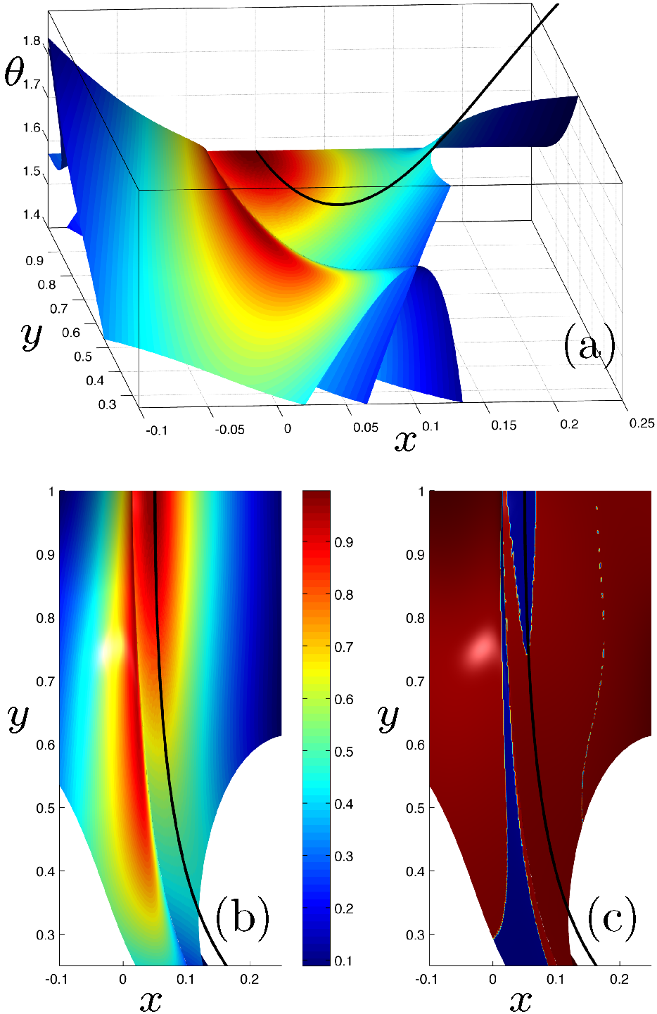
Figure 4: (color online) a) The two-dimensional shearless ($\psi=0$) surface embedded in the three-dimensional phase space. The coloring represents the two-dimensional bFTLE field on this surface. The Cauchy-Green integration time is $T=3$. The black curve is the stable BIM attached to the rightward propagating burning fixed point at the top of the channel. The computation of the isosurface is restricted to the computation box shown. b) A view of the bFTLE field on the shearless surface projected onto the $xy$-plane. The two white patches on the bottom left and right are where the shearless surface has exited the computation box. c) The sign of the bFTLE curvature normal to the shearless fronts (see Eq. (47). Blue is negative and red is positive.

We now apply the method of Sect. III to the steady wind case ($v_{w}=-0.15$) with the relatively short Cauchy-Green integration time $T=3$. We should find a bLCS that follows the initial length of the time-independent BIM. Before finding the bLCS, however, it is helpful to visualize the shearless surface. Fig. 4a shows the surface in 3D. For comparison, the stable BIM is shown in black. Near the burning fixed point, the BIM lies near (though not precisely within) the shearless surface. This is an important first check on the validity of our technique; if the BIM were far from the shearless surface, we would have no chance of recovering it.

At the bottom center of Fig. 4a is a “pitchfork” intersection between two branches of the surface. The differentiability of the $\psi$ field implies that the intersection curve between these two branches must be a shearless front, i.e. a trajectory of Eqs. (45). Thus, no shearless fronts may pass through this intersection.

The coloring in Figs. 4a and 4b represents the bFTLE field Eq. (50). Notice that the BIM follows a bFTLE ridge at the top of Fig. 4b, another critical check on our technique. Curiously, there is a second bFTLE ridge on the left in Fig. 4b. This ridge lies on a separate branch of the pitchfork structure, as seen in Fig. 4a.

We next identify those regions where the second derivative of the bFTLE field normal to the shearless curves is negative. Figure 4c illustrates the sign of this curvature, with blue representing negative and red representing positive. There are two regions of negative curvature, one for each of the bFTLE ridges. We focus on the rightmost region associated with the BIM.

We next compute shearless fronts, targeting the bFTLE ridge on the right. We select initial conditions using the intersection of the shearless surface with a plane normal to the BIM, yielding the bold line of initial points in Fig. 5a Note (1). We integrate Eqs. (45) upward toward the top of the channel and downward toward the bottom. Figures 5a and 5b show these shearless fronts in 3D and 2D, respectively.

We then compute the average normal repulsion, Eq. (51), along the segments of the shearless curves above the dashed line $y=0.7$ in Fig. 5b. This line is chosen to lie close to the bottom of the negative curvature region in Fig. 4c. The resulting average normal repulsion is shown in the inset of Fig. 5c. It exhibits a clear local maximum, which selects the red shearless curve isolated in Fig. 5c. This curve is the bLCS, and it faithfully follows the initial length of the BIM, as anticipated, before eventually deviating markedly from it.

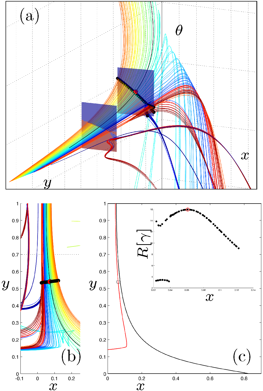
Figure 5: (color online) a) Shearless fronts computed for Cauchy-Green integration time $T=3$. The initial points (bold) of the trajectories were computed by intersecting a plane transverse to the BIM (at the red dot) with the shearless surface. The BIM is the thin black curve. b) The shearless fronts are shown projected onto the $xy$-plane. c-inset) Plot of the average normal repulsion, Eq. (51), as a function of the $x$-coordinate of the initial point for each trajectory in parts a and b. A smooth maximum is marked in red and determines which shearless front is the bLCS. c) The bLCS is plotted in red next to the BIM in black. The open circle marks the initial condition for generating the bLCS.

IV.3 The bLCS for a steady wind—long integration time

We extract a bLCS for the same dynamics as in Sect. IV.2 but for a longer Cauchy-Green integration time of $T=6$. The result is summarized in Fig. 6. Clearly the bLCS (red) closely tracks the BIM (black), considerably longer than for the $T=3$ case. In fact, the agreement is quite good all the way to the bottom of the channel. This is exactly what we expect to see as the integration time $T$ is increased.

Figure 6: (color online) The bLCS (red) and the BIM (black) for Cauchy-Green integration time $T=6$. The open circle on the bLCS marks the initial point used to integrate the shearless front. (The neighboring shearless fronts are not shown.) The inset shows the average repulsion on a shearless front as a function of the $x$-coordinate of its initial point. The average was computed along the shearless fronts above the dashed line at $y=0.2$.

V Conclusion

We have developed a technique to extract maximally repelling (or attracting) fronts, called burning Lagrangian coherent structures (bLCSs) for the finite-time dynamics of fronts evolving within a flowing fluid. We verified that this technique returns the burning invariant manifolds (BIMs) for the case of a time-independent flow. Clearly more work is needed to establish the relevance of these bLCSs to time-periodic and, most importantly, to time-aperiodic flows. This will be pursued in a separate publication.