Distributed Estimation of Graph Spectrum111This work was supported by the National Science Foundation under grant CMMI-0900806.

Mu Yang and Choon Yik Tang
School of Electrical and Computer Engineering
University of Oklahoma, Norman, OK 73019, USA
{muyangwz,cytang}@ou.edu
Abstract

In this paper, we develop a two-stage distributed algorithm that enables nodes in a graph to cooperatively estimate the spectrum of a matrix W𝑊W associated with the graph, which includes the adjacency and Laplacian matrices as special cases. In the first stage, the algorithm uses a discrete-time linear iteration and the Cayley-Hamilton theorem to convert the problem into one of solving a set of linear equations, where each equation is known to a node. In the second stage, if the nodes happen to know that W𝑊W is cyclic, the algorithm uses a Lyapunov approach to asymptotically solve the equations with an exponential rate of convergence. If they do not know whether W𝑊W is cyclic, the algorithm uses a random perturbation approach and a structural controllability result to approximately solve the equations with an error that can be made small. Finally, we provide simulation results that illustrate the algorithm.

1 Introduction

The spectrum of a graph, defined as the set of eigenvalues of either its adjacency or Laplacian matrix, provides a useful characterization of the properties of the graph. For instance, the distribution of such eigenvalues offers insights into the shapes and sizes of communities in a complex network [1]. As another example, the largest and smallest of such eigenvalues provides bounds on the maximum, minimum, and average node degrees [2]. The spectrum has also been used, for example, in chemistry, where it is associated with the stability of molecules [2], and in quantum mechanics, where it is related to the energy of Hamiltonian systems [2].

With the continued advances in technology that enable humans to build increasingly complex networks, it is becoming desirable that nodes in a network have the ability to analyze the network themselves, such as decentralizedly computing the spectrum of the network, so that valuable understanding about, say, the network structure may be gained. Motivated by this, a number of distributed algorithms have been proposed in the literature, including [3, 4, 5] that consider estimation of the entire spectrum of the Laplacian matrix, and [6, 7, 8] that focus on estimation of its second smallest eigenvalue (i.e., the algebraic connectivity).

In this paper, we add to the literature by developing a two-stage distributed algorithm, which enables nodes in a graph to cooperatively estimate the spectrum of a matrix W𝑊W associated with the graph. Unlike in [3, 4, 5, 6, 7, 8], the matrix W𝑊W can be the adjacency or Laplacian matrix of the graph, a weighted version of these matrices, or any other matrix induced by the graph (see Section 2). To construct the algorithm, we first use a discrete-time linear iteration and the Cayley-Hamilton theorem to convert the original problem into an equivalent problem of solving a set of linear equations of the form Ax=b𝐴𝑥𝑏Ax=b, where every row of A𝐴A and b𝑏b is known to a particular node (Section 3). We then show that the matrix A𝐴A can be made almost surely nonsingular if the nodes happen to know that W𝑊W is cyclic, but not necessarily so if they do not (Section 3). In the case of the former, we use a Lyapunov approach to asymptotically solve the equations with an exponential rate of convergence (Section 4). In the case of the latter, we use a random perturbation approach and a structural controllability result to approximately solve the equations with an error that can be made small (Section 5). Finally, we provide simulation results that illustrate our distributed algorithm (Section 6) and conclude the paper with a word on future research directions (Section 7).

2 Problem Formulation

Consider a network modeled as an undirected, connected graph 𝒢=(𝒱,)𝒢𝒱\mathcal{G}=(\mathcal{V},\mathcal{E}), where 𝒱={1,2,,N}𝒱12𝑁\mathcal{V}=\{1,2,\ldots,N\} denotes the set of N2𝑁2N\geq 2 nodes and {{i,j}:i,j𝒱,ij}conditional-set𝑖𝑗formulae-sequence𝑖𝑗𝒱𝑖𝑗\mathcal{E}\subset\{\{i,j\}:i,j\in\mathcal{V},i\neq j\} denotes the set of edges. Any two nodes i,j𝒱𝑖𝑗𝒱i,j\in\mathcal{V} are neighbors and can communicate if and only if {i,j}𝑖𝑗\{i,j\}\in\mathcal{E}. The set of neighbors of each node i𝒱𝑖𝒱i\in\mathcal{V} is denoted as 𝒩i={j𝒱:{i,j}}subscript𝒩𝑖conditional-set𝑗𝒱𝑖𝑗\mathcal{N}_{i}=\{j\in\mathcal{V}:\{i,j\}\in\mathcal{E}\}, and the communications are assumed to be delay- and error-free, with no quantization.

Suppose associated with the graph 𝒢𝒢\mathcal{G} is a square matrix W=[wij]N×N𝑊delimited-[]subscript𝑤𝑖𝑗superscript𝑁𝑁W=[w_{ij}]\in\mathbb{R}^{N\times N} satisfying the following assumption:

Assumption 1.

The matrix W𝑊W is such that for each i,j𝒱𝑖𝑗𝒱i,j\in\mathcal{V} with ij𝑖𝑗i\neq j, if {i,j}𝑖𝑗\{i,j\}\notin\mathcal{E}, then wij=wji=0subscript𝑤𝑖𝑗subscript𝑤𝑗𝑖0w_{ij}=w_{ji}=0.

Note that Assumption 1 allows wiisubscript𝑤𝑖𝑖w_{ii} i𝒱for-all𝑖𝒱\forall i\in\mathcal{V} to be arbitrary. It also allows wijsubscript𝑤𝑖𝑗w_{ij} and wjisubscript𝑤𝑗𝑖w_{ji} {i,j}for-all𝑖𝑗\forall\{i,j\}\in\mathcal{E} to be arbitrary and different. Thus, W𝑊W can be the adjacency or Laplacian matrix of graph 𝒢𝒢\mathcal{G}, a weighted version of these matrices, or any other matrix associated with 𝒢𝒢\mathcal{G} as long as Assumption 1 holds.

Suppose each node i𝒱𝑖𝒱i\in\mathcal{V} knows only 𝒩isubscript𝒩𝑖\mathcal{N}_{i}, wiisubscript𝑤𝑖𝑖w_{ii}, and wijsubscript𝑤𝑖𝑗w_{ij} j𝒩ifor-all𝑗subscript𝒩𝑖\forall j\in\mathcal{N}_{i}, which it prefers to not share with any of its neighbors due perhaps to security and privacy reasons. Yet, despite having only such local information about the graph 𝒢𝒢\mathcal{G} and matrix W𝑊W, suppose every node i𝒱𝑖𝒱i\in\mathcal{V} wants to determine the spectrum of W𝑊W, i.e., all the N𝑁N eigenvalues of W𝑊W, denoted as

λ(1),λ(2),,λ(N),superscript𝜆1superscript𝜆2superscript𝜆𝑁\displaystyle\lambda^{(1)},\lambda^{(2)},\ldots,\lambda^{(N)}\in\mathbb{C}, (1)

where complex eigenvalues must be in the form of conjugate pairs. Finally, suppose each node i𝒱𝑖𝒱i\in\mathcal{V} knows the value of N𝑁N, which is not an unreasonable assumption since each of them wants to determine the values of N𝑁N objects.

Given the above, the goal of this paper is to devise a distributed algorithm that enables every node i𝒱𝑖𝒱i\in\mathcal{V} to estimate the spectrum (1) of W𝑊W with a guaranteed accuracy.

3 Forming a Set of Linear Equations

In this section, we show that by having the nodes execute a discrete-time linear iteration N𝑁N times, the problem of finding the spectrum (1) of W𝑊W may be converted into one of solving a set of linear equations with appealing properties.

Observe that although none of the nodes has complete information about 𝒢𝒢\mathcal{G} and W𝑊W, each node i𝒱𝑖𝒱i\in\mathcal{V} knows the entire row i𝑖i of W𝑊W (since it knows wiisubscript𝑤𝑖𝑖w_{ii} and wijsubscript𝑤𝑖𝑗w_{ij} j𝒩ifor-all𝑗subscript𝒩𝑖\forall j\in\mathcal{N}_{i}, and since wij=0subscript𝑤𝑖𝑗0w_{ij}=0 j{i}𝒩ifor-all𝑗𝑖subscript𝒩𝑖\forall j\notin\{i\}\cup\mathcal{N}_{i} by Assumption 1). This makes the nodes well-suited to carry out the discrete-time linear iteration

yi(t+1)=wiiyi(t)+j𝒩iwijyj(t),i𝒱,t+,formulae-sequencesubscript𝑦𝑖𝑡1subscript𝑤𝑖𝑖subscript𝑦𝑖𝑡subscript𝑗subscript𝒩𝑖subscript𝑤𝑖𝑗subscript𝑦𝑗𝑡formulae-sequencefor-all𝑖𝒱for-all𝑡subscript\displaystyle y_{i}(t+1)=w_{ii}y_{i}(t)+\sum_{j\in\mathcal{N}_{i}}w_{ij}y_{j}(t),\quad\forall i\in\mathcal{V},\;\forall t\in\mathbb{Z}_{+}, (2)

which in matrix form may be written as

y(t+1)=Wy(t),t+,formulae-sequence𝑦𝑡1𝑊𝑦𝑡for-all𝑡subscript\displaystyle y(t+1)=Wy(t),\quad\forall t\in\mathbb{Z}_{+}, (3)

where +={0,1,2,}subscript012\mathbb{Z}_{+}=\{0,1,2,\ldots\}, yi(t)subscript𝑦𝑖𝑡y_{i}(t)\in\mathbb{R} is maintained in node i𝑖i’s local memory, and

y(t)=[y1(t)y2(t)yN(t)]TN.𝑦𝑡superscriptmatrixsubscript𝑦1𝑡subscript𝑦2𝑡subscript𝑦𝑁𝑡𝑇superscript𝑁\displaystyle y(t)=\begin{bmatrix}y_{1}(t)&y_{2}(t)&\cdots&y_{N}(t)\end{bmatrix}^{T}\in\mathbb{R}^{N}. (4)

Indeed, (2) or (3) can be implemented by having each node i𝒱𝑖𝒱i\in\mathcal{V} repeatedly send its yi(t)subscript𝑦𝑖𝑡y_{i}(t) to every neighbor j𝒩i𝑗subscript𝒩𝑖j\in\mathcal{N}_{i}.

Since (3) is a discrete-time linear system, we can write

y(t)=Wty(0),t+,formulae-sequence𝑦𝑡superscript𝑊𝑡𝑦0for-all𝑡subscript\displaystyle y(t)=W^{t}y(0),\quad\forall t\in\mathbb{Z}_{+}, (5)

so that

y(N)=WNy(0).𝑦𝑁superscript𝑊𝑁𝑦0\displaystyle y(N)=W^{N}y(0). (6)

By the Cayley-Hamilton theorem, WNsuperscript𝑊𝑁W^{N} in (6) may be expressed as

WN=x(0)INx(1)Wx(N1)WN1,superscript𝑊𝑁superscript𝑥0subscript𝐼𝑁superscript𝑥1𝑊superscript𝑥𝑁1superscript𝑊𝑁1\displaystyle W^{N}=-x^{(0)}I_{N}-x^{(1)}W-\cdots-x^{(N-1)}W^{N-1}, (7)

where Inn×nsubscript𝐼𝑛superscript𝑛𝑛I_{n}\in\mathbb{R}^{n\times n} is the identity matrix and the scalars x(0),x(1),,x(N1)superscript𝑥0superscript𝑥1superscript𝑥𝑁1x^{(0)},x^{(1)},\ldots,x^{(N-1)}\in\mathbb{R} are the N𝑁N coefficients of the characteristic polynomial of W𝑊W, i.e.,

det(λINW)=(λλ(1))(λλ(2))(λλ(N))det𝜆subscript𝐼𝑁𝑊𝜆superscript𝜆1𝜆superscript𝜆2𝜆superscript𝜆𝑁\displaystyle\operatorname{det}(\lambda I_{N}-W)=(\lambda-\lambda^{(1)})(\lambda-\lambda^{(2)})\cdots(\lambda-\lambda^{(N)})
=λN+x(N1)λN1++x(1)λ+x(0).absentsuperscript𝜆𝑁superscript𝑥𝑁1superscript𝜆𝑁1superscript𝑥1𝜆superscript𝑥0\displaystyle\quad=\lambda^{N}+x^{(N-1)}\lambda^{N-1}+\cdots+x^{(1)}\lambda+x^{(0)}. (8)

Substituting (7) into (6) and using (5), we obtain

y(N)𝑦𝑁\displaystyle y(N) =(x(0)INx(1)Wx(N1)WN1)y(0)absentsuperscript𝑥0subscript𝐼𝑁superscript𝑥1𝑊superscript𝑥𝑁1superscript𝑊𝑁1𝑦0\displaystyle=(-x^{(0)}I_{N}-x^{(1)}W-\cdots-x^{(N-1)}W^{N-1})y(0)
=x(0)y(0)x(1)y(1)x(N1)y(N1).absentsuperscript𝑥0𝑦0superscript𝑥1𝑦1superscript𝑥𝑁1𝑦𝑁1\displaystyle=-x^{(0)}y(0)-x^{(1)}y(1)-\cdots-x^{(N-1)}y(N-1). (9)

By using (4), we can rewrite (9) as

[y1(0)y1(1)y1(N1)y2(0)y2(1)y2(N1)yN(0)yN(1)yN(N1)]A[x(0)x(1)x(N1)]x=[y1(N)y2(N)yN(N)]b,subscriptmatrixsubscript𝑦10subscript𝑦11subscript𝑦1𝑁1subscript𝑦20subscript𝑦21subscript𝑦2𝑁1subscript𝑦𝑁0subscript𝑦𝑁1subscript𝑦𝑁𝑁1𝐴subscriptmatrixsuperscript𝑥0superscript𝑥1superscript𝑥𝑁1superscript𝑥subscriptmatrixsubscript𝑦1𝑁subscript𝑦2𝑁subscript𝑦𝑁𝑁𝑏\displaystyle\underbrace{\begin{bmatrix}y_{1}(0)&y_{1}(1)&\cdots&y_{1}(N-1)\\ y_{2}(0)&y_{2}(1)&\cdots&y_{2}(N-1)\\ \vdots&\vdots&\ddots&\vdots\\ y_{N}(0)&y_{N}(1)&\cdots&y_{N}(N-1)\end{bmatrix}}_{A}\underbrace{\begin{bmatrix}x^{(0)}\\ x^{(1)}\\ \vdots\\ x^{(N-1)}\end{bmatrix}}_{x^{*}}=\underbrace{\begin{bmatrix}-y_{1}(N)\\ -y_{2}(N)\\ \vdots\\ -y_{N}(N)\end{bmatrix}}_{b}, (10)

where, for later convenience, we denote the matrix on the left-hand side of (10) as AN×N𝐴superscript𝑁𝑁A\in\mathbb{R}^{N\times N}, the vector of characteristic polynomial coefficients as xNsuperscript𝑥superscript𝑁x^{*}\in\mathbb{R}^{N}, and the vector on the right-hand side of (10) as bN𝑏superscript𝑁b\in\mathbb{R}^{N}.

The matrix equation (10) suggests the following approach for finding the spectrum (1) of W𝑊W: suppose each node i𝒱𝑖𝒱i\in\mathcal{V} selects an initial condition yi(0)subscript𝑦𝑖0y_{i}(0)\in\mathbb{R}. Upon selecting the yi(0)subscript𝑦𝑖0y_{i}(0)’s, suppose the nodes execute the discrete-time linear iteration (2) or equivalently (3) N𝑁N times for t{0,1,,N1}𝑡01𝑁1t\in\{0,1,\ldots,N-1\}. During the execution, suppose each node i𝒱𝑖𝒱i\in\mathcal{V} stores the resulting N+1𝑁1N+1 numbers yi(0),yi(1),,yi(N1),yi(N)subscript𝑦𝑖0subscript𝑦𝑖1subscript𝑦𝑖𝑁1subscript𝑦𝑖𝑁y_{i}(0),y_{i}(1),\ldots,y_{i}(N-1),y_{i}(N) in its local memory. Then, (10) is a set of N𝑁N linear equations in which each node i𝒱𝑖𝒱i\in\mathcal{V} knows the entire row i𝑖i of A𝐴A and b𝑏b, and in which the vector xsuperscript𝑥x^{*} of N𝑁N characteristic polynomial coefficients x(0),x(1),,x(N1)superscript𝑥0superscript𝑥1superscript𝑥𝑁1x^{(0)},x^{(1)},\ldots,x^{(N-1)} of W𝑊W are the N𝑁N unknowns. It follows that if A𝐴A is nonsingular, and if the nodes are able to cooperatively solve (10) for the unique xsuperscript𝑥x^{*}, then each of them could determine on its own the N𝑁N eigenvalues λ(1),λ(2),,λ(N)superscript𝜆1superscript𝜆2superscript𝜆𝑁\lambda^{(1)},\lambda^{(2)},\ldots,\lambda^{(N)} of W𝑊W using (8) and a polynomial root-finding algorithm.

To realize the above approach, it is necessary that A𝐴A in (10) is nonsingular. To see whether this can be ensured, observe from (4), (5), and (10) that A𝐴A may be expressed as

A=[y(0)Wy(0)WN1y(0)].𝐴matrix𝑦0𝑊𝑦0superscript𝑊𝑁1𝑦0\displaystyle A=\begin{bmatrix}y(0)&Wy(0)&\cdots&W^{N-1}y(0)\end{bmatrix}. (11)

In the form (11), A𝐴A is, interestingly, the controllability matrix of a fictitious discrete-time single-input linear system

z(t+1)=Wz(t)+y(0)u(t),t+,formulae-sequence𝑧𝑡1𝑊𝑧𝑡𝑦0𝑢𝑡for-all𝑡subscript\displaystyle z(t+1)=Wz(t)+y(0)u(t),\quad\forall t\in\mathbb{Z}_{+}, (12)

where z(t)N𝑧𝑡superscript𝑁z(t)\in\mathbb{R}^{N} is its state, u(t)𝑢𝑡u(t)\in\mathbb{R} is its input, W𝑊W is its state matrix, and y(0)𝑦0y(0) is its input matrix. Hence:

Proposition 1.

The matrix A𝐴A in (10) or (11) is nonsingular if and only if the pair (W,y(0))𝑊𝑦0(W,y(0)) of the system (12) is controllable.

Since W𝑊W is given by the problem but y(0)𝑦0y(0) may be freely selected by the nodes, it may be possible to select y(0)𝑦0y(0) so that the pair (W,y(0))𝑊𝑦0(W,y(0)) is controllable. The following definition and lemmas examine this possibility:

Definition 1 (​​[9]).

A square matrix with real entries is said to be cyclic if each of its distinct eigenvalues has a geometric multiplicity of 111.

Lemma 1.

If W𝑊W is not cyclic, then for every y(0)N𝑦0superscript𝑁y(0)\in\mathbb{R}^{N}, the pair (W,y(0))𝑊𝑦0(W,y(0)) is not controllable.

Proof.

Suppose W𝑊W is not cyclic and let y(0)N𝑦0superscript𝑁y(0)\in\mathbb{R}^{N} be given. Then, by Definition 1, W𝑊W has an eigenvalue λ𝜆\lambda\in\mathbb{C} whose geometric multiplicity exceeds 111, i.e., rank(WλIN)<N1rank𝑊𝜆subscript𝐼𝑁𝑁1\operatorname{rank}(W-\lambda I_{N})<N-1. Since y(0)𝑦0y(0) is a column vector, rank([WλIN|y(0)])<Nrankdelimited-[]𝑊conditional𝜆subscript𝐼𝑁𝑦0𝑁\operatorname{rank}([W-\lambda I_{N}\;|\;y(0)])<N. Therefore, by statements (i) and (iv) of Theorem 3.1 in [9], the pair (W,y(0))𝑊𝑦0(W,y(0)) is not controllable. ∎

Lemma 2.

If W𝑊W is cyclic, then for almost every y(0)N𝑦0superscript𝑁y(0)\in\mathbb{R}^{N}, the pair (W,y(0))𝑊𝑦0(W,y(0)) is controllable.

Proof.

According to Lemma 3.12 in [9], if 𝒜n×n𝒜superscript𝑛𝑛\mathcal{A}\in\mathbb{R}^{n\times n} is cyclic and n×msuperscript𝑛𝑚\mathcal{B}\in\mathbb{R}^{n\times m} is such that the pair (𝒜,)𝒜(\mathcal{A},\mathcal{B}) is controllable, then for almost every vm𝑣superscript𝑚v\in\mathbb{R}^{m}, the pair (𝒜,v)𝒜𝑣(\mathcal{A},\mathcal{B}v) is controllable. Applying this lemma with 𝒜=W𝒜𝑊\mathcal{A}=W, =INsubscript𝐼𝑁\mathcal{B}=I_{N}, and v=y(0)𝑣𝑦0v=y(0), and using the fact that the pair (W,IN)𝑊subscript𝐼𝑁(W,I_{N}) is controllable, we conclude that so is the pair (W,y(0))𝑊𝑦0(W,y(0)). ∎

Proposition 1 and Lemma 1 imply that W𝑊W being cyclic is necessary for A𝐴A in (10) or (11) to be nonsingular. Lemma 2, on the other hand, implies that W𝑊W being cyclic is essentially sufficient because almost every y(0)N𝑦0superscript𝑁y(0)\in\mathbb{R}^{N} would work. This latter result is especially useful in a decentralized network because the result allows each node i𝒱𝑖𝒱i\in\mathcal{V} to select its yi(0)subscript𝑦𝑖0y_{i}(0)\in\mathbb{R} independently from other nodes and randomly from any continuous probability distribution before executing (2) or (3), and be almost sure that the resulting A𝐴A would be nonsingular.

Motivated by the above analysis, in the rest of this paper we consider separately the following two scenarios:

Scenario 1.

The nodes know that W𝑊W is cyclic.

Scenario 2.

The nodes do not know whether W𝑊W is cyclic, or know that W𝑊W is not cyclic.

We consider Scenarios 1 and 2 separately because Scenario 1 is easier to deal with (in Section 4) and its treatment helps us deal with Scenario 2 (in Section 5). We note that both of these scenarios arise in applications. For instance, if the graph 𝒢𝒢\mathcal{G} represents a sensor network and the entries wiisubscript𝑤𝑖𝑖w_{ii} i𝒱for-all𝑖𝒱\forall i\in\mathcal{V} and wijsubscript𝑤𝑖𝑗w_{ij} {i,j}for-all𝑖𝑗\forall\{i,j\}\in\mathcal{E} of W𝑊W represent random sensor measurements with continuous probability distributions, then Scenario 1 takes place as the nodes could say with near certainty that W𝑊W is cyclic because almost every n𝑛n-by-n𝑛n matrix has n𝑛n distinct eigenvalues and, thus, is cyclic. In contrast, if W𝑊W represents the adjacency or Laplacian matrix of 𝒢𝒢\mathcal{G}, then Scenario 2 takes place as W𝑊W would be cyclic if 𝒢𝒢\mathcal{G} is, say, a path graph [2] and would not be cyclic if 𝒢𝒢\mathcal{G} is, say, a complete or cycle graph [2], which the nodes could not tell because they only have local information about 𝒢𝒢\mathcal{G}.

To summarize, in this section we have transformed the problem of finding the spectrum (1) of W𝑊W into one of solving the set of linear equations (10), in which each node i𝒱𝑖𝒱i\in\mathcal{V} knows the entire row i𝑖i of A𝐴A and b𝑏b, and in which A𝐴A can be made almost surely nonsingular in Scenario 1, but not necessarily so in Scenario 2.

4 Solving the Set of Linear Equations in Scenario 1

In this section, we focus on Scenario 1 and develop a continuous-time distributed algorithm that enables the nodes to asymptotically solve the set of linear equations (10) with an exponential rate of convergence.

To facilitate the development, we assume that the nodes have executed (2) or (3) to arrive at (10). Moreover, since A𝐴A in (10) can be made almost surely nonsingular in this Scenario 1, we assume that it is nonsingular throughout the section. With these assumptions, for each i𝒱𝑖𝒱i\in\mathcal{V} let ai=[yi(0)yi(1)yi(N1)]TNsubscript𝑎𝑖superscriptmatrixsubscript𝑦𝑖0subscript𝑦𝑖1subscript𝑦𝑖𝑁1𝑇superscript𝑁a_{i}=\begin{bmatrix}y_{i}(0)&y_{i}(1)&\cdots&y_{i}(N-1)\end{bmatrix}^{T}\in\mathbb{R}^{N} and bi=yi(N)subscript𝑏𝑖subscript𝑦𝑖𝑁b_{i}=-y_{i}(N)\in\mathbb{R}, so that (10) may be stated as

[a1Ta2TaNT]A[x(0)x(1)x(N1)]x=[b1b2bN]b,subscriptmatrixsuperscriptsubscript𝑎1𝑇superscriptsubscript𝑎2𝑇superscriptsubscript𝑎𝑁𝑇𝐴subscriptmatrixsuperscript𝑥0superscript𝑥1superscript𝑥𝑁1superscript𝑥subscriptmatrixsubscript𝑏1subscript𝑏2subscript𝑏𝑁𝑏\displaystyle\underbrace{\begin{bmatrix}\;\text{---}\;a_{1}^{T}\;\text{---}\;\\ \;\text{---}\;a_{2}^{T}\;\text{---}\;\\ \vdots\\ \;\text{---}\;a_{N}^{T}\;\text{---}\;\end{bmatrix}}_{A}\underbrace{\begin{bmatrix}x^{(0)}\\ x^{(1)}\\ \vdots\\ x^{(N-1)}\end{bmatrix}}_{x^{*}}=\underbrace{\begin{bmatrix}b_{1}\\ b_{2}\\ \vdots\\ b_{N}\end{bmatrix}}_{b}, (13)

where aisubscript𝑎𝑖a_{i} and bisubscript𝑏𝑖b_{i} are known to node i𝑖i because (2) or (3) has been executed. In addition to knowing aisubscript𝑎𝑖a_{i} and bisubscript𝑏𝑖b_{i}, suppose each node i𝒱𝑖𝒱i\in\mathcal{V} maintains in its local memory an estimate xi(t)=[xi(0)(t)xi(1)(t)xi(N1)(t)]TNsubscript𝑥𝑖𝑡superscriptmatrixsuperscriptsubscript𝑥𝑖0𝑡superscriptsubscript𝑥𝑖1𝑡superscriptsubscript𝑥𝑖𝑁1𝑡𝑇superscript𝑁x_{i}(t)=\begin{bmatrix}x_{i}^{(0)}(t)&x_{i}^{(1)}(t)&\cdots&x_{i}^{(N-1)}(t)\end{bmatrix}^{T}\in\mathbb{R}^{N} of the unknown, unique solution xNsuperscript𝑥superscript𝑁x^{*}\in\mathbb{R}^{N}, where here t[0,)𝑡0t\in[0,\infty) denotes continuous-time (unlike in Section 3 where t+𝑡subscriptt\in\mathbb{Z}_{+} denotes discrete-time). Furthermore, let 𝐱(t)=(x1(t),x2(t),,xN(t))N2𝐱𝑡subscript𝑥1𝑡subscript𝑥2𝑡subscript𝑥𝑁𝑡superscriptsuperscript𝑁2\mathbf{x}(t)=(x_{1}(t),x_{2}(t),\ldots,x_{N}(t))\in\mathbb{R}^{N^{2}} and 𝐱=(x,x,,x)N2superscript𝐱superscript𝑥superscript𝑥superscript𝑥superscriptsuperscript𝑁2\mathbf{x}^{*}=(x^{*},x^{*},\ldots,x^{*})\in\mathbb{R}^{N^{2}} be vectors obtained by stacking the N𝑁N estimates xi(t)subscript𝑥𝑖𝑡x_{i}(t)’s and N𝑁N copies of the solution xsuperscript𝑥x^{*}.

To come up with a distributed algorithm that gradually drives 𝐱(t)𝐱𝑡\mathbf{x}(t) to 𝐱superscript𝐱\mathbf{x}^{*}, consider a quadratic Lyapunov function candidate V:N2:𝑉superscriptsuperscript𝑁2V:\mathbb{R}^{N^{2}}\rightarrow\mathbb{R}, defined as

V(𝐱)=i𝒱αi(aiTxibi)2+{i,j}β{i,j}(xixj)T(xixj),𝑉𝐱subscript𝑖𝒱subscript𝛼𝑖superscriptsuperscriptsubscript𝑎𝑖𝑇subscript𝑥𝑖subscript𝑏𝑖2subscript𝑖𝑗subscript𝛽𝑖𝑗superscriptsubscript𝑥𝑖subscript𝑥𝑗𝑇subscript𝑥𝑖subscript𝑥𝑗\displaystyle V(\mathbf{x})=\sum_{i\in\mathcal{V}}\alpha_{i}(a_{i}^{T}x_{i}-b_{i})^{2}+\sum_{\{i,j\}\in\mathcal{E}}\beta_{\{i,j\}}(x_{i}-x_{j})^{T}(x_{i}-x_{j}), (14)

where αi>0subscript𝛼𝑖0\alpha_{i}>0 i𝒱for-all𝑖𝒱\forall i\in\mathcal{V} and β{i,j}>0subscript𝛽𝑖𝑗0\beta_{\{i,j\}}>0 {i,j}for-all𝑖𝑗\forall\{i,j\}\in\mathcal{E} are parameters. Notice that each term in the first summation in (14) is a measure of how far away from the hyperplane {zN:aiTz=bi}conditional-set𝑧superscript𝑁superscriptsubscript𝑎𝑖𝑇𝑧subscript𝑏𝑖\{z\in\mathbb{R}^{N}:a_{i}^{T}z=b_{i}\} the estimate xi(t)subscript𝑥𝑖𝑡x_{i}(t) is. Moreover, because A𝐴A is nonsingular and because of (13), the N𝑁N hyperplanes {zN:aiTz=bi}conditional-set𝑧superscript𝑁superscriptsubscript𝑎𝑖𝑇𝑧subscript𝑏𝑖\{z\in\mathbb{R}^{N}:a_{i}^{T}z=b_{i}\} i𝒱for-all𝑖𝒱\forall i\in\mathcal{V} have a unique intersection at xsuperscript𝑥x^{*}. Furthermore, the second summation in (14) is a measure of the disagreement among the estimates xi(t)subscript𝑥𝑖𝑡x_{i}(t)’s. Hence, both the first and second summations in (14) are only positive semidefinite functions of 𝐱𝐱\mathbf{x}. However, as the following proposition shows, adding them up makes V𝑉V a legitimate Lyapunov function candidate:

Proposition 2.

If A𝐴A in (13) is nonsingular, then the function V𝑉V in (14) is positive definite with respect to 𝐱superscript𝐱\mathbf{x}^{*}.

Proof.

Clearly, V𝑉V is a positive semidefinite function of 𝐱𝐱\mathbf{x}. To show that it is positive definite with respect to 𝐱superscript𝐱\mathbf{x}^{*}, we show that V(𝐱)=0𝑉𝐱0V(\mathbf{x})=0 if and only if 𝐱=𝐱𝐱superscript𝐱\mathbf{x}=\mathbf{x}^{*}. Suppose 𝐱=𝐱𝐱superscript𝐱\mathbf{x}=\mathbf{x}^{*}. Then, aiTxibi=0superscriptsubscript𝑎𝑖𝑇subscript𝑥𝑖subscript𝑏𝑖0a_{i}^{T}x_{i}-b_{i}=0 i𝒱for-all𝑖𝒱\forall i\in\mathcal{V} according to (13). In addition, the second summation in (14) drops out. Therefore, V(𝐱)=0𝑉𝐱0V(\mathbf{x})=0. Next, suppose V(𝐱)=0𝑉𝐱0V(\mathbf{x})=0. Then,

aiTxisuperscriptsubscript𝑎𝑖𝑇subscript𝑥𝑖\displaystyle a_{i}^{T}x_{i} =bi,i𝒱,formulae-sequenceabsentsubscript𝑏𝑖for-all𝑖𝒱\displaystyle=b_{i},\quad\forall i\in\mathcal{V}, (15)
xisubscript𝑥𝑖\displaystyle x_{i} =xj,{i,j}.formulae-sequenceabsentsubscript𝑥𝑗for-all𝑖𝑗\displaystyle=x_{j},\quad\forall\{i,j\}\in\mathcal{E}. (16)

Since 𝒢𝒢\mathcal{G} is connected, (16) implies that there exists x~N~𝑥superscript𝑁\tilde{x}\in\mathbb{R}^{N} such that xi=x~subscript𝑥𝑖~𝑥x_{i}=\tilde{x} i𝒱for-all𝑖𝒱\forall i\in\mathcal{V}. Substituting this into (15), we get aiTx~=bisuperscriptsubscript𝑎𝑖𝑇~𝑥subscript𝑏𝑖a_{i}^{T}\tilde{x}=b_{i} i𝒱for-all𝑖𝒱\forall i\in\mathcal{V} or, equivalently, Ax~=b𝐴~𝑥𝑏A\tilde{x}=b. Since A𝐴A is nonsingular, we have x~=x~𝑥superscript𝑥\tilde{x}=x^{*}, so that 𝐱=𝐱𝐱superscript𝐱\mathbf{x}=\mathbf{x}^{*}. ∎

Remark 1.

Notice that V𝑉V in (14) can also be written as

V(𝐱)=(𝐱𝐱)TP(𝐱𝐱),𝑉𝐱superscript𝐱superscript𝐱𝑇𝑃𝐱superscript𝐱\displaystyle V(\mathbf{x})=(\mathbf{x}-\mathbf{x}^{*})^{T}P(\mathbf{x}-\mathbf{x}^{*}),

where P=PTN2×N2𝑃superscript𝑃𝑇superscriptsuperscript𝑁2superscript𝑁2P=P^{T}\in\mathbb{R}^{N^{2}\times N^{2}} is positive definite and given by

P=[α1a1a1T0α2a2a2T0αNaNaNT]+LβIN,𝑃matrixsubscript𝛼1subscript𝑎1superscriptsubscript𝑎1𝑇missing-subexpressionmissing-subexpression0missing-subexpressionsubscript𝛼2subscript𝑎2superscriptsubscript𝑎2𝑇missing-subexpressionmissing-subexpressionmissing-subexpressionmissing-subexpressionmissing-subexpression0missing-subexpressionmissing-subexpressionsubscript𝛼𝑁subscript𝑎𝑁superscriptsubscript𝑎𝑁𝑇tensor-productsubscript𝐿𝛽subscript𝐼𝑁\displaystyle P=\begin{bmatrix}\alpha_{1}a_{1}a_{1}^{T}&&&0\\ &\alpha_{2}a_{2}a_{2}^{T}&&\\ &&\ddots&\\ 0&&&\alpha_{N}a_{N}a_{N}^{T}\end{bmatrix}+L_{\beta}\otimes I_{N},

where tensor-product\otimes denotes the Kronecker product and Lβ=[Lij]N×Nsubscript𝐿𝛽delimited-[]subscript𝐿𝑖𝑗superscript𝑁𝑁L_{\beta}=[L_{ij}]\in\mathbb{R}^{N\times N} is a weighted Laplacian matrix of 𝒢𝒢\mathcal{G} with Lii=j𝒩iβ{i,j}subscript𝐿𝑖𝑖subscript𝑗subscript𝒩𝑖subscript𝛽𝑖𝑗L_{ii}=\sum_{j\in\mathcal{N}_{i}}\beta_{\{i,j\}}, Lij=β{i,j}subscript𝐿𝑖𝑗subscript𝛽𝑖𝑗L_{ij}=-\beta_{\{i,j\}} if {i,j}𝑖𝑗\{i,j\}\in\mathcal{E}, and Lij=0subscript𝐿𝑖𝑗0L_{ij}=0 if ij𝑖𝑗i\neq j and {i,j}𝑖𝑗\{i,j\}\notin\mathcal{E}.∎

With Proposition 2 in hand, we next take the time derivative of V𝑉V along the state trajectory 𝐱(t)𝐱𝑡\mathbf{x}(t) to obtain

V˙(𝐱(t))=2i𝒱[αi(aiTxi(t)bi)ai+j𝒩iβ{i,j}(xi(t)xj(t))]x˙i(t),t[0,).formulae-sequence˙𝑉𝐱𝑡2subscript𝑖𝒱delimited-[]subscript𝛼𝑖superscriptsubscript𝑎𝑖𝑇subscript𝑥𝑖𝑡subscript𝑏𝑖subscript𝑎𝑖subscript𝑗subscript𝒩𝑖subscript𝛽𝑖𝑗subscript𝑥𝑖𝑡subscript𝑥𝑗𝑡subscript˙𝑥𝑖𝑡for-all𝑡0\displaystyle\dot{V}(\mathbf{x}(t))=2\sum_{i\in\mathcal{V}}\Bigl{[}\alpha_{i}(a_{i}^{T}x_{i}(t)-b_{i})a_{i}+\sum_{j\in\mathcal{N}_{i}}\beta_{\{i,j\}}(x_{i}(t)-x_{j}(t))\Bigr{]}\dot{x}_{i}(t),\quad\forall t\in[0,\infty). (17)

Examining (17), we see that V˙(𝐱(t))˙𝑉𝐱𝑡\dot{V}(\mathbf{x}(t)) can be made negative semidefinite—at the very least—by letting each x˙i(t)subscript˙𝑥𝑖𝑡\dot{x}_{i}(t) be the negative of the expression within the brackets in (17), i.e.,

x˙i(t)=αi(aiTxi(t)bi)aij𝒩iβ{i,j}(xi(t)xj(t)),i𝒱,t[0,).formulae-sequencesubscript˙𝑥𝑖𝑡subscript𝛼𝑖superscriptsubscript𝑎𝑖𝑇subscript𝑥𝑖𝑡subscript𝑏𝑖subscript𝑎𝑖subscript𝑗subscript𝒩𝑖subscript𝛽𝑖𝑗subscript𝑥𝑖𝑡subscript𝑥𝑗𝑡formulae-sequencefor-all𝑖𝒱for-all𝑡0\displaystyle\dot{x}_{i}(t)=-\alpha_{i}(a_{i}^{T}x_{i}(t)-b_{i})a_{i}-\sum_{j\in\mathcal{N}_{i}}\beta_{\{i,j\}}(x_{i}(t)-x_{j}(t)),\quad\forall i\in\mathcal{V},\;\forall t\in[0,\infty). (18)

The following theorem asserts that the continuous-time system (18) possesses an excellent property:

Theorem 1.

If A𝐴A in (13) is nonsingular, then the system (18) has a unique equilibrium point at 𝐱superscript𝐱\mathbf{x}^{*} that is globally exponentially stable, so that 𝐱(0)N2for-all𝐱0superscriptsuperscript𝑁2\forall\mathbf{x}(0)\in\mathbb{R}^{N^{2}}, limt𝐱(t)=𝐱subscript𝑡𝐱𝑡superscript𝐱\lim_{t\rightarrow\infty}\mathbf{x}(t)=\mathbf{x}^{*}, i.e., limtxi(t)=xsubscript𝑡subscript𝑥𝑖𝑡superscript𝑥\lim_{t\rightarrow\infty}x_{i}(t)=x^{*} i𝒱for-all𝑖𝒱\forall i\in\mathcal{V}.

Proof.

For each i𝒱𝑖𝒱i\in\mathcal{V}, setting x˙i(t)subscript˙𝑥𝑖𝑡\dot{x}_{i}(t) in (18) to zero yields

0=αi(aiTxibi)aij𝒩iβ{i,j}(xixj).0subscript𝛼𝑖superscriptsubscript𝑎𝑖𝑇subscript𝑥𝑖subscript𝑏𝑖subscript𝑎𝑖subscript𝑗subscript𝒩𝑖subscript𝛽𝑖𝑗subscript𝑥𝑖subscript𝑥𝑗\displaystyle 0=-\alpha_{i}(a_{i}^{T}x_{i}-b_{i})a_{i}-\sum_{j\in\mathcal{N}_{i}}\beta_{\{i,j\}}(x_{i}-x_{j}). (19)

Summing both sides of (19) over i𝒱𝑖𝒱i\in\mathcal{V} gives

0=i𝒱αi(aiTxibi)ai.0subscript𝑖𝒱subscript𝛼𝑖superscriptsubscript𝑎𝑖𝑇subscript𝑥𝑖subscript𝑏𝑖subscript𝑎𝑖\displaystyle 0=\sum_{i\in\mathcal{V}}-\alpha_{i}(a_{i}^{T}x_{i}-b_{i})a_{i}. (20)

Due to (13) and to A𝐴A being nonsingular, the vectors a1,a2,,aNsubscript𝑎1subscript𝑎2subscript𝑎𝑁a_{1},a_{2},\ldots,a_{N} in (20) are linearly independent in Nsuperscript𝑁\mathbb{R}^{N}. Thus,

0=αi(aiTxibi),i𝒱.formulae-sequence0subscript𝛼𝑖superscriptsubscript𝑎𝑖𝑇subscript𝑥𝑖subscript𝑏𝑖for-all𝑖𝒱\displaystyle 0=-\alpha_{i}(a_{i}^{T}x_{i}-b_{i}),\quad\forall i\in\mathcal{V}. (21)

Substituting (21) back into (19) results in

0=j𝒩iβ{i,j}(xixj),i𝒱,formulae-sequence0subscript𝑗subscript𝒩𝑖subscript𝛽𝑖𝑗subscript𝑥𝑖subscript𝑥𝑗for-all𝑖𝒱\displaystyle 0=\sum_{j\in\mathcal{N}_{i}}\beta_{\{i,j\}}(x_{i}-x_{j}),\quad\forall i\in\mathcal{V},

which is equivalent to

0=(LβIN)𝐱,0tensor-productsubscript𝐿𝛽subscript𝐼𝑁𝐱\displaystyle 0=(L_{\beta}\otimes I_{N})\mathbf{x}, (22)

where tensor-product\otimes and Lβsubscript𝐿𝛽L_{\beta} have been defined in Remark 1. Since 𝒢𝒢\mathcal{G} is connected, (22) implies that xi=x~subscript𝑥𝑖~𝑥x_{i}=\tilde{x} i𝒱for-all𝑖𝒱\forall i\in\mathcal{V} for some x~N~𝑥superscript𝑁\tilde{x}\in\mathbb{R}^{N}. Plugging this into (21) yields aiTx~=bisuperscriptsubscript𝑎𝑖𝑇~𝑥subscript𝑏𝑖a_{i}^{T}\tilde{x}=b_{i} i𝒱for-all𝑖𝒱\forall i\in\mathcal{V}. Since A𝐴A is nonsingular, we have x~=x~𝑥superscript𝑥\tilde{x}=x^{*}, i.e., 𝐱=𝐱𝐱superscript𝐱\mathbf{x}=\mathbf{x}^{*}. Hence, the system (18) has a unique equilibrium point at 𝐱superscript𝐱\mathbf{x}^{*}. Since for each i𝒱𝑖𝒱i\in\mathcal{V} the right-hand side of (18) is the negative of the expression within the brackets in (17), V˙(𝐱(t))˙𝑉𝐱𝑡\dot{V}(\mathbf{x}(t)) is negative definite with respect to 𝐱superscript𝐱\mathbf{x}^{*}. Therefore, the equilibrium point 𝐱superscript𝐱\mathbf{x}^{*} is globally exponentially stable. ∎

Having established Theorem 1, we now relate it back to the original problem of finding the spectrum (1) of W𝑊W. To this end, suppose each node i𝒱𝑖𝒱i\in\mathcal{V} maintains in its local memory an estimate λi()(t)superscriptsubscript𝜆𝑖𝑡\lambda_{i}^{(\ell)}(t)\in\mathbb{C} of the unknown, \ellth eigenvalue λ()superscript𝜆\lambda^{(\ell)} of W𝑊W for {1,2,,N}12𝑁\ell\in\{1,2,\ldots,N\}. Also suppose at each time t[0,)𝑡0t\in[0,\infty), node i𝑖i lets its N𝑁N estimates λi()(t)superscriptsubscript𝜆𝑖𝑡\lambda_{i}^{(\ell)}(t)’s be the roots of an N𝑁Nth-order polynomial formed by the estimate xi(t)=[xi(0)(t)xi(1)(t)xi(N1)(t)]Tsubscript𝑥𝑖𝑡superscriptmatrixsuperscriptsubscript𝑥𝑖0𝑡superscriptsubscript𝑥𝑖1𝑡superscriptsubscript𝑥𝑖𝑁1𝑡𝑇x_{i}(t)=\begin{bmatrix}x_{i}^{(0)}(t)&x_{i}^{(1)}(t)&\cdots&x_{i}^{(N-1)}(t)\end{bmatrix}^{T} that is also stored in its local memory, i.e.,

(λλi(1)(t))(λλi(2)(t))(λλi(N)(t))𝜆superscriptsubscript𝜆𝑖1𝑡𝜆superscriptsubscript𝜆𝑖2𝑡𝜆superscriptsubscript𝜆𝑖𝑁𝑡\displaystyle(\lambda-\lambda_{i}^{(1)}(t))(\lambda-\lambda_{i}^{(2)}(t))\cdots(\lambda-\lambda_{i}^{(N)}(t))
=λN+xi(N1)(t)λN1++xi(1)(t)λ+xi(0)(t),i𝒱,t[0,),formulae-sequenceabsentsuperscript𝜆𝑁superscriptsubscript𝑥𝑖𝑁1𝑡superscript𝜆𝑁1superscriptsubscript𝑥𝑖1𝑡𝜆superscriptsubscript𝑥𝑖0𝑡formulae-sequencefor-all𝑖𝒱for-all𝑡0\displaystyle\quad=\lambda^{N}+x_{i}^{(N-1)}(t)\lambda^{N-1}+\cdots+x_{i}^{(1)}(t)\lambda+x_{i}^{(0)}(t),\quad\forall i\in\mathcal{V},\;\forall t\in[0,\infty), (23)

which can be implemented using a polynomial root-finding algorithm embedded in node i𝑖i. Then, because (λ(1),λ(2),,λ(N))superscript𝜆1superscript𝜆2superscript𝜆𝑁(\lambda^{(1)},\lambda^{(2)},\ldots,\lambda^{(N)}) in (8) is a continuous function of xsuperscript𝑥x^{*}, and (λi(1)(t),λi(2)(t),,λi(N)(t))superscriptsubscript𝜆𝑖1𝑡superscriptsubscript𝜆𝑖2𝑡superscriptsubscript𝜆𝑖𝑁𝑡(\lambda_{i}^{(1)}(t),\lambda_{i}^{(2)}(t),\ldots,\lambda_{i}^{(N)}(t)) in (23) is the same continuous function of xi(t)subscript𝑥𝑖𝑡x_{i}(t), Theorem 1 implies that

limtλi()(t)=λ(),i𝒱,{1,2,,N}.formulae-sequencesubscript𝑡superscriptsubscript𝜆𝑖𝑡superscript𝜆formulae-sequencefor-all𝑖𝒱for-all12𝑁\displaystyle\lim_{t\rightarrow\infty}\lambda_{i}^{(\ell)}(t)=\lambda^{(\ell)},\quad\forall i\in\mathcal{V},\;\forall\ell\in\{1,2,\ldots,N\}. (24)

Equation (24), in turn, implies that the system (18) is a continuous-time distributed algorithm that enables the nodes to asymptotically learn the spectrum (1) of W𝑊W.

Putting together the development in Sections 3 and 4, we obtain the following two-stage distributed algorithm, which is applicable to this Scenario 1:

Algorithm 1 (For Scenario 1).
  • 1.

    Each node i𝒱𝑖𝒱i\in\mathcal{V} selects its yi(0)subscript𝑦𝑖0y_{i}(0)\in\mathbb{R} independently from other nodes and randomly from any continuous probability distribution.

  • 2.

    Upon completion, the nodes execute (2) or (3) N𝑁N times for t{0,1,,N1}𝑡01𝑁1t\in\{0,1,\ldots,N-1\}, so that each node i𝒱𝑖𝒱i\in\mathcal{V} gradually learns the entire row i𝑖i of A𝐴A and b𝑏b in (10).

  • 3.

    Upon completion, the nodes execute (18) and (23) for t[0,)𝑡0t\in[0,\infty), so that each node i𝒱𝑖𝒱i\in\mathcal{V} is able to continuously update its xi(t)subscript𝑥𝑖𝑡x_{i}(t) and λi()(t)superscriptsubscript𝜆𝑖𝑡\lambda_{i}^{(\ell)}(t)’s. \blacksquare

Remark 2.

The current literature offers a few distributed algorithms [10, 11] that may be used to solve linear equations (10). These algorithms are different from (18) in that they force the state of each node to stay in an affine set, whereas (18) allows the state to freely roam the state space.∎

5 Solving the Set of Linear Equations in Scenario 2

In this section, we focus on Scenario 2 and provide a slightly different algorithm that enables the nodes to approximately solve (10) with an error that can be made small.

Recall that Scenario 2 represents a situation where the nodes either do not know whether W𝑊W is cyclic, or somehow know that W𝑊W is not cyclic. Consequently, they either do not know whether A𝐴A in (10) is nonsingular, or know that A𝐴A is singular. Although the nodes could still apply Algorithm 1, there is no guarantee that their estimates xi(t)subscript𝑥𝑖𝑡x_{i}(t)’s would converge to xsuperscript𝑥x^{*}. One way to address this issue is to have the nodes randomly perturb the matrix W𝑊W and vector y(0)𝑦0y(0), so that the resulting A𝐴A in (11) is hopefully nonsingular. Of course, such a random perturbation approach no longer allows them to asymptotically determine the exact spectrum of W𝑊W. However, getting an estimate of the spectrum of W𝑊W may be sufficient in some applications. Thus, we will adopt this random perturbation approach in this Scenario 2.

For notational simplicity, let the matrix associated with the graph 𝒢𝒢\mathcal{G} be denoted as W¯=[w¯ij]N×N¯𝑊delimited-[]subscript¯𝑤𝑖𝑗superscript𝑁𝑁\overline{W}=[\overline{w}_{ij}]\in\mathbb{R}^{N\times N} instead of W=[wij]𝑊delimited-[]subscript𝑤𝑖𝑗W=[w_{ij}], and let W𝑊W instead denote a perturbed version of W¯¯𝑊\overline{W}. In addition, let x¯()superscript¯𝑥\overline{x}^{(\ell)}’s and λ¯()superscript¯𝜆\overline{\lambda}^{(\ell)}’s denote, respectively, the characteristic polynomial coefficients and eigenvalues of W¯¯𝑊\overline{W} that the nodes wish to determine, and let x()superscript𝑥x^{(\ell)}’s and λ()superscript𝜆\lambda^{(\ell)}’s denote those of W𝑊W as before. Moreover, let the perturbed matrix W𝑊W be obtained from W¯¯𝑊\overline{W} in a decentralized manner as follows: prior to executing (2) or (3), each node i𝒱𝑖𝒱i\in\mathcal{V} lets

wiisubscript𝑤𝑖𝑖\displaystyle w_{ii} =w¯ii+δii,i𝒱,formulae-sequenceabsentsubscript¯𝑤𝑖𝑖subscript𝛿𝑖𝑖for-all𝑖𝒱\displaystyle=\overline{w}_{ii}+\delta_{ii},\quad\forall i\in\mathcal{V}, (25)
wijsubscript𝑤𝑖𝑗\displaystyle w_{ij} =w¯ij+δij,i𝒱,j𝒩i,formulae-sequenceabsentsubscript¯𝑤𝑖𝑗subscript𝛿𝑖𝑗formulae-sequencefor-all𝑖𝒱for-all𝑗subscript𝒩𝑖\displaystyle=\overline{w}_{ij}+\delta_{ij},\quad\forall i\in\mathcal{V},\;\forall j\in\mathcal{N}_{i}, (26)

where the δiisubscript𝛿𝑖𝑖\delta_{ii}’s and δijsubscript𝛿𝑖𝑗\delta_{ij}’s are independent, uniformly distributed random variables in the interval [a,a]𝑎𝑎[-a,a], so that a>0𝑎0a>0 represents the perturbation magnitude. Notice that since w¯ij=0subscript¯𝑤𝑖𝑗0\overline{w}_{ij}=0 i𝒱for-all𝑖𝒱\forall i\in\mathcal{V} j{i}𝒩ifor-all𝑗𝑖subscript𝒩𝑖\forall j\notin\{i\}\cup\mathcal{N}_{i} by Assumption 1,

wij=0,i𝒱,j{i}𝒩iformulae-sequencesubscript𝑤𝑖𝑗0formulae-sequencefor-all𝑖𝒱for-all𝑗𝑖subscript𝒩𝑖\displaystyle w_{ij}=0,\quad\forall i\in\mathcal{V},\;\forall j\notin\{i\}\cup\mathcal{N}_{i} (27)

as well. Also note that because the nodes are slated to select their yi(0)subscript𝑦𝑖0y_{i}(0)’s independently and randomly from a continuous probability distribution, there is no need to further randomly perturb these yi(0)subscript𝑦𝑖0y_{i}(0)’s.

The following lemma uses a structural controllability result to show that the aforementioned approach is effective:

Lemma 3.

If W𝑊W is as defined in (25)–(27) and y(0)𝑦0y(0) is as defined in Step 1 of Algorithm 1, then A𝐴A in (11) is almost surely nonsingular.

Proof.

Reconsider the graph 𝒢=(𝒱,)𝒢𝒱\mathcal{G}=(\mathcal{V},\mathcal{E}) from Section 2. Let 𝒮={(𝒜,)N×N×N:𝒜ij=0ifijand{i,j}}𝒮conditional-set𝒜superscript𝑁𝑁superscript𝑁subscript𝒜𝑖𝑗0if𝑖𝑗and𝑖𝑗\mathcal{S}=\{(\mathcal{A},\mathcal{B})\in\mathbb{R}^{N\times N}\times\mathbb{R}^{N}:\mathcal{A}_{ij}=0\;\text{if}\;i\neq j\;\text{and}\;\{i,j\}\notin\mathcal{E}\} and 𝒮c={(𝒜,)𝒮:(𝒜,)is controllable}𝒮subscript𝒮𝑐conditional-set𝒜𝒮𝒜is controllable𝒮\mathcal{S}_{c}=\{(\mathcal{A},\mathcal{B})\in\mathcal{S}:(\mathcal{A},\mathcal{B})\;\text{is controllable}\}\subset\mathcal{S}. In addition, let 𝒜=diag(1,2,,N)N×Nsuperscript𝒜diag12𝑁superscript𝑁𝑁\mathcal{A}^{*}=\operatorname{diag}(1,2,\ldots,N)\in\mathbb{R}^{N\times N} and Nsuperscriptsuperscript𝑁\mathcal{B}^{*}\in\mathbb{R}^{N} be the all-one vector. Then, (𝒜,)𝒮superscript𝒜superscript𝒮(\mathcal{A}^{*},\mathcal{B}^{*})\in\mathcal{S} according to the definition of 𝒮𝒮\mathcal{S}. Moreover, (𝒜,)𝒮csuperscript𝒜superscriptsubscript𝒮𝑐(\mathcal{A}^{*},\mathcal{B}^{*})\in\mathcal{S}_{c} because the controllability matrix formed by (𝒜,)superscript𝒜superscript(\mathcal{A}^{*},\mathcal{B}^{*}) is a Vandermonde matrix that is nonsingular. These two properties of (𝒜,)superscript𝒜superscript(\mathcal{A}^{*},\mathcal{B}^{*}), along with the definition of structural controllability [12], imply that every (𝒜,)𝒮𝒜𝒮(\mathcal{A},\mathcal{B})\in\mathcal{S} is structurally controllable. Next, let (𝒜,)𝒮𝒜𝒮(\mathcal{A},\mathcal{B})\in\mathcal{S} and ϵ>0italic-ϵ0\epsilon>0 be given. Then, by Proposition 1 of [12], there exists (𝒜c,c)𝒮csubscript𝒜𝑐subscript𝑐subscript𝒮𝑐(\mathcal{A}_{c},\mathcal{B}_{c})\in\mathcal{S}_{c} such that 𝒜𝒜c<ϵnorm𝒜subscript𝒜𝑐italic-ϵ\|\mathcal{A}-\mathcal{A}_{c}\|<\epsilon and c<ϵnormsubscript𝑐italic-ϵ\|\mathcal{B}-\mathcal{B}_{c}\|<\epsilon. Hence, 𝒮csubscript𝒮𝑐\mathcal{S}_{c} is a dense subset of 𝒮𝒮\mathcal{S}. Lastly, note that (W,y(0))𝒮𝑊𝑦0𝒮(W,y(0))\in\mathcal{S} due to Assumption 1, (25)–(27), and Step 1 of Algorithm 1. Since 𝒮csubscript𝒮𝑐\mathcal{S}_{c} is a dense subset of 𝒮𝒮\mathcal{S}, (W,y(0))𝑊𝑦0(W,y(0)) is almost surely in 𝒮csubscript𝒮𝑐\mathcal{S}_{c}. Therefore, by Proposition 1, A𝐴A in (11) is almost surely nonsingular. ∎

As it follows from Lemma 3, by having the nodes perform the extra step described in (25)–(27), the results developed in Sections 3 and 4 become applicable to this Scenario 2. Furthermore, because both the characteristic polynomial coefficients and eigenvalues of a matrix are continuous functions of its entries, by having the nodes decrease the perturbation magnitude a𝑎a toward zero, the differences between the x()superscript𝑥x^{(\ell)}’s and λ()superscript𝜆\lambda^{(\ell)}’s of W𝑊W and the x¯()superscript¯𝑥\overline{x}^{(\ell)}’s and λ¯()superscript¯𝜆\overline{\lambda}^{(\ell)}’s of W¯¯𝑊\overline{W} can be made arbitrarily small, at least in principle. Note, however, that numerical issues may arise when a𝑎a is too small, or when the resulting A𝐴A is ill-conditioned. At present, we do not have answers to these numerical issues, and we believe they are important future research directions.

Based on the above, we obtain the following two-stage distributed algorithm for this Scenario 2:

Algorithm 2 (For Scenario 2).
  • 1.

    Each node i𝒱𝑖𝒱i\in\mathcal{V} executes (25)–(27) to obtain a perturbed matrix W𝑊W.

  • 2.

    The remaining steps are identical to those of Algorithm 1. \blacksquare

6 Simulation Results

In this section, we present two sets of simulation results that demonstrate the effectiveness of Algorithm 1 for Scenario 1 and Algorithm 2 for Scenario 2.

6.1 Simulation of Algorithm 1 for Scenario 1
Refer to caption
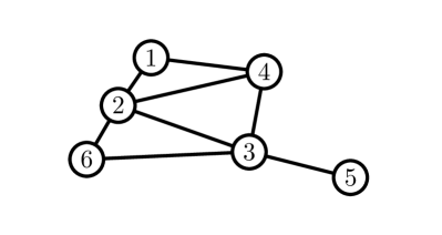
(a) A 666-node graph.
Refer to caption
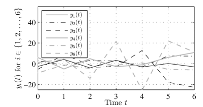
(b) Data points yi(t)subscript𝑦𝑖𝑡y_{i}(t) for i{1,2,,6}𝑖126i\in\{1,2,\ldots,6\} and t{0,1,,6}𝑡016t\in\{0,1,\ldots,6\} that form the set of linear equations (10).
Refer to caption
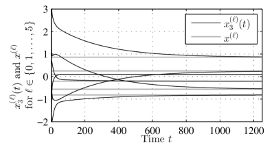
(c) Node 333’s estimate x3()(t)superscriptsubscript𝑥3𝑡x_{3}^{(\ell)}(t) of the \ellth characteristic polynomial coefficient x()superscript𝑥x^{(\ell)} for {0,1,,5}015\ell\in\{0,1,\ldots,5\}.
Refer to caption
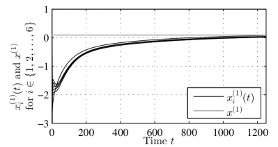
(d) Node i𝑖i’s estimate xi(1)(t)superscriptsubscript𝑥𝑖1𝑡x_{i}^{(1)}(t) of the 111st characteristic polynomial coefficient x(1)superscript𝑥1x^{(1)} for i{1,2,,6}𝑖126i\in\{1,2,\ldots,6\}.
Figure 1: Performance of Algorithm 1 for Scenario 1.

Consider a sensor network with N=6𝑁6N=6 nodes, modeled as an undirected, connected graph 𝒢𝒢\mathcal{G}, whose topology is shown in Figure 1(a). Suppose associated with the graph 𝒢𝒢\mathcal{G} is a 666-by-666 matrix W𝑊W, whose entries satisfy Assumption 1 and represent random sensor measurements given by

W=[0.100.2400.78000.240.530.390.0400.1900.340.211.150.130.710.260.210.320.5400000.4500.39000.470.84001.35].𝑊matrix0.100.2400.78000.240.530.390.0400.1900.340.211.150.130.710.260.210.320.5400000.4500.39000.470.84001.35\displaystyle W=\begin{bmatrix}-0.10&-0.24&0&0.78&0&0\\ 0.24&0.53&0.39&-0.04&0&-0.19\\ 0&0.34&0.21&1.15&-0.13&0.71\\ -0.26&-0.21&0.32&-0.54&0&0\\ 0&0&-0.45&0&0.39&0\\ 0&0.47&-0.84&0&0&-1.35\end{bmatrix}.

Assuming that such measurements are realizations of continuously distributed random variables, the nodes are almost certain that W𝑊W is cyclic, so that Scenario 1 takes place. Thus, to determine all the eigenvalues λ()superscript𝜆\lambda^{(\ell)}’s of W𝑊W, which are given by 1.02±0.55iplus-or-minus1.020.55𝑖-1.02\pm 0.55i, 0.004±0.46iplus-or-minus0.0040.46𝑖-0.004\pm 0.46i, 0.380.380.38, and 0.810.810.81, the nodes may apply Algorithm 1.

Figures 1(b)–1(d) display the result of simulating Algorithm 1 with αi=10subscript𝛼𝑖10\alpha_{i}=10 i𝒱for-all𝑖𝒱\forall i\in\mathcal{V} and β{i,j}=10subscript𝛽𝑖𝑗10\beta_{\{i,j\}}=10 {i,j}for-all𝑖𝑗\forall\{i,j\}\in\mathcal{E}. Specifically, Figure 1(b) shows the data points yi(t)subscript𝑦𝑖𝑡y_{i}(t) for i{1,2,,6}𝑖126i\in\{1,2,\ldots,6\} and t{0,1,,6}𝑡016t\in\{0,1,\ldots,6\} that are used to form the set of linear equations (10). Figure 1(c) shows, as a function of time t𝑡t, node 333’s estimate x3()(t)superscriptsubscript𝑥3𝑡x_{3}^{(\ell)}(t) of the \ellth characteristic polynomial coefficient x()superscript𝑥x^{(\ell)} of W𝑊W for {0,1,,5}015\ell\in\{0,1,\ldots,5\}. Likewise, Figure 1(d) shows node i𝑖i’s estimate xi(1)(t)superscriptsubscript𝑥𝑖1𝑡x_{i}^{(1)}(t) of the 111st coefficient x(1)superscript𝑥1x^{(1)} for i{1,2,,6}𝑖126i\in\{1,2,\ldots,6\}. (Due to space limitation, we are unable to include plots of xi()(t)superscriptsubscript𝑥𝑖𝑡x_{i}^{(\ell)}(t) for all i{1,2,,6}𝑖126i\in\{1,2,\ldots,6\} and {0,1,,5}015\ell\in\{0,1,\ldots,5\}.) Observe that despite having only local information about 𝒢𝒢\mathcal{G} and W𝑊W, the nodes are able to utilize Algorithm 1 to asymptotically determine all the characteristic polynomial coefficients x()superscript𝑥x^{(\ell)}’s of W𝑊W and, hence, all its eigenvalues λ()superscript𝜆\lambda^{(\ell)}’s.

6.2 Simulation of Algorithm 2 for Scenario 2
Refer to caption
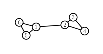
(a) A 666-node graph.
Refer to caption
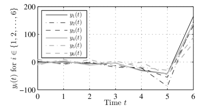
(b) Data points yi(t)subscript𝑦𝑖𝑡y_{i}(t) for i{1,2,,6}𝑖126i\in\{1,2,\ldots,6\} and t{0,1,,6}𝑡016t\in\{0,1,\ldots,6\} that form the set of linear equations (10).
Refer to caption
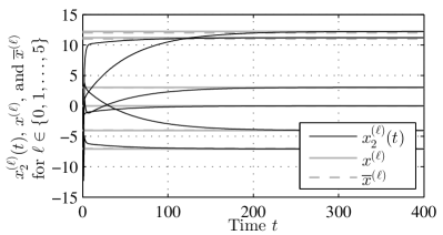
(c) Node 222’s estimate x2()(t)superscriptsubscript𝑥2𝑡x_{2}^{(\ell)}(t) of the \ellth perturbed and true characteristic polynomial coefficients x()superscript𝑥x^{(\ell)} and x¯()superscript¯𝑥\overline{x}^{(\ell)} for {0,1,,5}015\ell\in\{0,1,\ldots,5\}.
Refer to caption
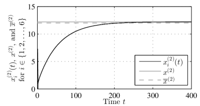
(d) Node i𝑖i’s estimate xi(2)(t)superscriptsubscript𝑥𝑖2𝑡x_{i}^{(2)}(t) of the 222nd perturbed and true characteristic polynomial coefficients x(2)superscript𝑥2x^{(2)} and x¯(2)superscript¯𝑥2\overline{x}^{(2)} for i{1,2,,6}𝑖126i\in\{1,2,\ldots,6\}.
Figure 2: Performance of Algorithm 2 for Scenario 2.

Consider next an undirected, connected graph 𝒢𝒢\mathcal{G} with N=6𝑁6N=6 nodes, whose topology is shown in Figure 2(a). Let W¯¯𝑊\overline{W} represent the adjacency matrix of 𝒢𝒢\mathcal{G} and suppose the nodes wish to determine all the eigenvalues λ¯()superscript¯𝜆\overline{\lambda}^{(\ell)}’s of W¯¯𝑊\overline{W}, which are given by 1.731.73-1.73, 11-1, 11-1, 0.410.41-0.41, 1.731.731.73, and 2.412.412.41. Because they only have local information about 𝒢𝒢\mathcal{G}, the nodes do not know whether W¯¯𝑊\overline{W} is cyclic, so that Scenario 2 takes place. (In fact, W¯¯𝑊\overline{W} in this particular example is not cyclic because it is symmetric and has repeated eigenvalues, at 11-1.) Therefore, the nodes have to apply Algorithm 2. In doing so, they let the perturbation magnitude be a=0.2𝑎0.2a=0.2 and obtain from (25)–(27) a perturbed matrix W𝑊W given by

W=[01.04001.010.940.9801.041.120000.9801.060000.951.010000.9800001.010.970000.920],𝑊matrix01.04001.010.940.9801.041.120000.9801.060000.951.010000.9800001.010.970000.920\displaystyle W=\begin{bmatrix}0&1.04&0&0&1.01&0.94\\ 0.98&0&1.04&1.12&0&0\\ 0&0.98&0&1.06&0&0\\ 0&0.95&1.01&0&0&0\\ 0.98&0&0&0&0&1.01\\ 0.97&0&0&0&0.92&0\end{bmatrix},

whose eigenvalues λ()superscript𝜆\lambda^{(\ell)}’s are 1.741.74-1.74, 0.970.97-0.97, 1.031.03-1.03, 0.400.40-0.40, 1.731.731.73, and 2.432.432.43, which are all distinct and slightly different from the eigenvalues λ¯()superscript¯𝜆\overline{\lambda}^{(\ell)}’s of W¯¯𝑊\overline{W}.

Figures 2(b)–2(d) display the result of simulating Algorithm 2 with αi=100subscript𝛼𝑖100\alpha_{i}=100 i𝒱for-all𝑖𝒱\forall i\in\mathcal{V} and β{i,j}=10subscript𝛽𝑖𝑗10\beta_{\{i,j\}}=10 {i,j}for-all𝑖𝑗\forall\{i,j\}\in\mathcal{E}, using a format similar to that of Figures 1(b)–1(d). The only difference is that Figures 2(c) and 2(d) show not only the characteristic polynomial coefficients x()superscript𝑥x^{(\ell)}’s of the “perturbed” W𝑊W, but also the characteristic polynomial coefficients x¯()superscript¯𝑥\overline{x}^{(\ell)}’s of the “true” W¯¯𝑊\overline{W}. Observe that with Algorithm 2, the nodes are able to asymptotically determine the x()superscript𝑥x^{(\ell)}’s and λ()superscript𝜆\lambda^{(\ell)}’s. In other words, they are able to approximately calculate the x¯()superscript¯𝑥\overline{x}^{(\ell)}’s and λ¯()superscript¯𝜆\overline{\lambda}^{(\ell)}’s with small errors.

7 Conclusion

In this paper, we have designed and analyzed a two-stage distributed algorithm that enables nodes in a graph to cooperatively estimate the graph spectrum. We have shown that asymptotically accurate estimation can be achieved if the nodes know that the associated matrix is cyclic, and estimation with small errors can be achieved if they do not. As for future research, we believe that making the algorithm numerically more robust, so that it can cope with poorly conditioned W𝑊W and A𝐴A, is an important next step.

References

  • [1] M. E. J. Newman, Networks: An Introduction.   New York, NY: Oxford University Press, 2010.
  • [2] F. R. K. Chung, Spectral Graph Theory.   American Mathematical Society, 1997.
  • [3] T. Sahai, A. Speranzon, and A. Banaszuk, “Hearing the clusters of a graph: A distributed algorithm,” Automatica, vol. 48, no. 1, pp. 15–24, 2012.
  • [4] M. Franceschelli, A. Gasparri, A. Giua, and C. Seatzu, “Decentralized estimation of Laplacian eigenvalues in multi-agent systems,” Automatica, vol. 49, no. 4, pp. 1031–1036, 2013.
  • [5] T.-M. D. Tran and A. Y. Kibangou, “Distributed estimation of graph Laplacian eigenvalues by the alternating direction of multipliers method,” in Proc. IFAC World Congress, Cape Town, South Africa, 2014, pp. 5526–5531.
  • [6] P. Yang, R. A. Freeman, G. J. Gordon, K. M. Lynch, S. S. Srinivasa, and R. Sukthankar, “Decentralized estimation and control of graph connectivity for mobile sensor networks,” Automatica, vol. 46, no. 2, pp. 390–396, 2010.
  • [7] R. Aragues, G. Shi, D. V. Dimarogonas, C. Sagues, and K. H. Johansson, “Distributed algebraic connectivity estimation for adaptive event-triggered consensus,” in Proc. American Control Conference, Montreal, Canada, 2012, pp. 32–37.
  • [8] C. Li and Z. Qu, “Distributed estimation of algebraic connectivity of directed networks,” Systems & Control Letters, vol. 62, no. 6, pp. 517–524, 2013.
  • [9] K. Zhou, J. C. Doyle, and K. Glover, Robust and Optimal Control.   Upper Saddle River, NJ: Prentice Hall, 1996.
  • [10] A. Nedić, A. Ozdaglar, and P. A. Parrilo, “Constrained consensus and optimization in multi-agent networks,” IEEE Transactions on Automatic Control, vol. 55, no. 4, pp. 922–938, 2010.
  • [11] S. Mou and A. S. Morse, “A fixed-neighbor, distributed algorithm for solving a linear algebraic equation,” in Proc. European Control Conference, Zurich, Switzerland, 2013, pp. 2269–2273.
  • [12] C.-T. Lin, “Structural controllability,” IEEE Transactions on Automatic Control, vol. 19, no. 3, pp. 201–208, 1974.