Compton Scattering from the Deuteron below Pion-Production Threshold

Abstract

Differential cross sections for elastic scattering of photons from the deuteron have recently been measured at the Tagged-Photon Facility at the MAX IV Laboratory in Lund, Sweden. These first new measurements in more than a decade further constrain the isoscalar electromagnetic polarizabilities of the nucleon and provide the first-ever results above 100 MeV, where the sensitivity to the polarizabilities is increased. We add 23 points between 70 and 112 MeV, at angles $60^{\circ}$, $120^{\circ}$ and $150^{\circ}$. Analysis of these data using a Chiral Effective Field Theory indicates that the cross sections are both self-consistent and consistent with previous measurements. Extracted values of $\alpha_{s}$ = [12.1 $\pm$ 0.8(stat) $\pm$ 0.2(BSR) $\pm$ 0.8(th)] $\times$ 10^-4 fm³ and $\beta_{s}$ = [2.4 $\pm$ 0.8(stat) $\pm$ 0.2(BSR) $\pm$ 0.8(th)] $\times$ 10^-4 fm³ are obtained from a fit to these 23 new data points. This paper presents in detail the experimental conditions and the data analysis used to extract the cross sections.

I Introduction

A new result on the extraction of the nucleon electromagnetic polarizabilities was recently reported, based on recent measurements of Compton scattering from the deuteron L.S. Myers et al. (2014a). This paper presents in detail the motivation, configuration, data analysis and critical evaluation of the experiment reported therein, as well as a parameter extraction using only the new data.

Low-energy nuclear Compton scattering $\gamma X\to\gamma X$ explores how the internal degrees of freedom of the target behave in the electric and magnetic fields of a real external photon. Since these fields induce radiation multipoles by displacing the target constituents, the energy dependence of the emitted radiation provides a stringent test of the symmetries and strengths which govern the interactions of the constituents with each other and with the photon; see e.g. a recent review H.W. Grießhammer et al. (2012).

The proton response can be measured directly and cleanly using a ${}^{1}\mathrm{H}$ target. The neutron, however, is much more difficult to study because it is unstable outside the nucleus and its coupling to photons is much weaker. Embedding the neutron into a stable nucleus allows its two-photon response to be reconstructed. An added benefit of this approach is that the signal from the neutron is enhanced through its interference with the contributions from the charged proton. It also enables one to probe how the photons couple to the charged pion-exchange currents which provide the bulk of nuclear binding. The deuteron, which is the simplest stable few-nucleon system, is an ideal target for Compton-scattering experiments as it provides a conceptually clean probe of our understanding of both single-hadron and few-nucleon physics at low energies.

After subtracting binding effects, theorists utilize such data to extract the two-photon response of the individual nucleon to the static fields; see H.W. Grießhammer et al. (2012); Hildebrandt et al. (2004) for details. First, one subtracts the Powell amplitudes J.L. Powell (1949) for photon scattering on a point-like spin-$\nicefrac{{1}}{{2}}$ nucleon with an anomalous magnetic moment. The remainder is then expanded into energy-dependent radiation multipoles of the incident and outgoing photon fields. Finally, these coefficients are extrapolated to the values at zero photon frequency $\omega$. In that limit, the leading contributions are quadratic in $\omega$. Their coefficients are called the static electric dipole polarizability $\alpha_{E1}$ and the static magnetic dipole polarizability $\beta_{M1}$ and can be separated by different angular dependences. They parametrize the stiffness of the nucleon against $E1\to E1$ and $M1\to M1$ transitions at zero photon energy, respectively.

A host of information about the hadron response is thus compressed into $\alpha_{E1}$ and $\beta_{M1}$, often referred to as “the polarizabilities”. They are experimentally not directly accessible since assumptions about the energy dependence and conventions on how to separate one- and two-photon physics enter. Nonetheless, they summarize information on the entire spectrum of nucleonic excitations. By comparing the quantities extracted from data with fully dynamical lattice QCD extractions which are anticipated in the near future Lujan et al. (2014a, b); Detmold et al. (2012), the polarizabilities will offer a stringent test of our understanding of Quantum Chromodynamics (QCD). Most notable is the opportunity to explore the two degrees of freedom with the lowest excitation energy, namely the pion cloud around the nucleon and the $\Delta(1232)$ excitation. Since both of these are dominated by isospin-symmetric interactions, differences between proton and neutron polarizabilities signal the breaking of isospin and chiral symmetry, in concert with such effects from short-distance physics. Besides being fundamental nucleon properties, $\alpha_{E1}$ and $\beta_{M1}$ also play a role in theoretical studies of the Lamb shift of muonic hydrogen and of the proton-neutron mass difference, and dominate the uncertainties of both Pachucki (1999); Carlson and Vanderhaeghen (2011); Birse and McGovern (2012); Walker-Loud et al. (2012).

As recently reviewed in Ref. H.W. Grießhammer et al. (2012), a statistically consistent proton Compton-scattering database contains a cornucopia of points between $30$ and $170$ MeV, with good angular coverage and statistical uncertainties usually around $5$%. Based on this extensive set, McGovern et al. McGovern et al. (2013) extracted the proton polarizabilities in Chiral Effective Field Theory ($\chi$EFT), the extension of Chiral Perturbation Theory to include baryons, as

$$\begin{split}&\alpha_{p}=10.65\pm 0.35(\text{stat})\pm 0.2(\text{BSR})\pm 0.3(\text{th})\\ &\beta_{p}=3.15\mp 0.35(\text{stat})\pm 0.2(\text{BSR})\mp 0.3(\text{th}),\end{split}$$ (1)

with $\chi^{2}=113.2$ for $135$ degrees of freedom. Theoretical uncertainties are separated from those induced by application of the Baldin Sum Rule (BSR) for the proton A.M. Baldin (1960). The BSR is a variant of the optical theorem which uses proton photoabsorption cross-section data to provide the constraint that $\alpha_{p}+\beta_{p}=13.8\pm 0.4$ Olmos de León et al. (2001).

By contrast, the neutron polarizabilities, as extracted from deuteron Compton scattering, are poorly determined. The calculations related to neutron polarizabilities appear to be theoretically well under control H.W. Grießhammer et al. (2012), but the experimental deuteron data are of smaller quantity and poorer quality than those of the proton. Three experiments have thus far constituted the world data: the pioneering effort of Lucas et al. at $49$ and $69$ MeV M.A. Lucas (1994); the follow-up measurement by Lundin et al. Lundin et al. (2003) which covered similar energies and angles; and the extension to $95$ MeV by Hornidge et al. D.L. Hornidge et al. (2000). This statistically consistent database contains only $29$ data points at $4$ energies between $49$ and $95$ MeV, with limited angular coverage, typical statistical uncertainties of more than $7$%, and typical systematic uncertainties in excess of $4$%. From these data, the isoscalar (average) nucleon polarizabilities were extracted using the same $\chi$EFT methodology as for the proton as

$$\begin{split}&\alpha_{s}=10.9\pm 0.9(\text{stat})\pm 0.2(\text{BSR})\pm 0.8(\text{th})\\ &\beta_{s}=3.6\mp 0.9(\text{stat})\pm 0.2(\text{BSR})\mp 0.8(\text{th}),\end{split}$$ (2)

with $\chi^{2}=24.2$ for $25$ degrees of freedom H.W. Grießhammer et al. (2012). The result is again constrained by a BSR for the nucleon. The isoscalar value

$$\alpha_{s}+\beta_{s}=14.5\pm 0.4$$ (3)

is found by combining the proton BSR above with empirical partial-wave amplitudes for pion photoproduction on the neutron which lead to the neutron sum rule $\alpha_{n}+\beta_{n}=15.2\pm 0.4$ M.I. Levchuk and A.I. L’vov (2000). The uncertainty in the neutron BSR is highly correlated with that for the proton.

Combining isoscalar and proton polarizabilities, Eqs. (1) and (2), leads to neutron values

$$\begin{split}&\alpha_{n}=11.1\pm 1.8(\text{stat})\pm 0.2(\text{BSR})\pm 0.8(\text{th})\\ &\beta_{n}=4.1\mp 1.8(\text{stat})\pm 0.2(\text{BSR})\mp 0.8(\text{th}),\end{split}$$ (4)

which are clearly dominated by the statistical uncertainties, which in turn are much larger than for the proton; see Eq. (1).

An alternative extraction of neutron polarizabilities from the 7 data points measured in quasi-elastic ²H($\gamma$,$\gamma^{\prime}$$n$)$p$ above 200 MeV Kossert et al. (2003) is consistent with these numbers. Again using the neutron BSR constraint, one finds:

$$\begin{split}&\alpha_{n}=12.5\pm 1.8(\text{stat}){}^{+1.1}_{-0.6}(\text{sys})\pm 1.1(\text{th})\\ &\beta_{n}=2.7\mp 1.8(\text{stat}){}_{-1.1}^{+0.6}(\text{sys})\mp 1.1(\text{th}),\end{split}$$ (5)

where the theory uncertainty may be underestimated L’vov . No extractions from heavier nuclei exist; good Compton data is available on ⁶Li L.S. Myers et al. (2012, 2014b), but comparable data have not been published for any other few-nucleon systems. A third technique, extracting the neutron polarizabilities from scattering from the Coulomb field of heavy nuclei, appears to be plagued by poorly understood systematic effects; see e.g. H.W. Grießhammer et al. (2012).

New deuteron data of good quality and reproducible systematic uncertainties are therefore necessary to see commonalities and differences in the two-photon responses of protons and neutrons. The experiment detailed in this paper effectively doubled the deuteron Compton database and significantly reduced the uncertainties of the neutron polarizabilities. These data overlap the previous sets at lower energies and add points up to $112$ MeV, with statistical and systematic uncertainties on par with preceding measurements. The extension to higher energies is particularly important since the sensitivity of the cross sections to the polarizabilities increases roughly with the square of the photon energy.

The resulting augmented world database is statistically consistent and recently resulted in a new extraction of the isoscalar polarizabilities in Refs. L.S. Myers et al. (2014a); fut as

$$\begin{split}&\alpha_{s}=11.1\pm 0.6(\text{stat})\pm 0.2(\text{BSR})\pm 0.8(\text{th})\\ &\beta_{s}=3.4\mp 0.6(\text{stat})\pm 0.2(\text{BSR})\mp 0.8(\text{th}).\end{split}$$ (6)

Our new measurement thus reduces the statistical uncertainties in $\alpha_{s}$ and $\beta_{s}$ by a factor of $1/3$. For the very first time, the uncertainty is now dominated by the theoretical uncertainties of the extraction.

While some aspects of our findings have been summarized briefly in a recent publication L.S. Myers et al. (2014a), we now provide a more detailed description of the entire experimental effort, including complementary information to aid in the interpretation of the results. In Sections II and III, we present the experimental setup at MAX IV and the data-analysis process, and pay special attention to yield corrections and systematic uncertainties. Section IV contains the resulting cross sections and an extraction of the polarizabilities, focusing on the self-consistency of this data set and its agreement with previous measurements.

II Experiment

The experiment was performed at the Tagged-Photon Facility J.-O. Adler et al. (2013) located at the MAX IV Laboratory Eriksson (2014) in Lund, Sweden. A pulse-stretched electron beam L.-J. Lindgren (2002) with a typical current of 15 nA and a duty factor of 45% was used to produce quasi-monoenergetic photons via the bremsstrahlung-tagging technique J.-O. Adler et al. (1990, 1997). The basic parameters of the electron and resulting tagged-photon beams are given in Table 1 for the first and second run periods, RP1 and RP2. An overview of the experimental layout is shown in Fig. 1.

Table 1: Basic parameters of the electron beam and the tagged-photon beam for the two run periods, RP1 and RP2.

	RP1	RP2
$E_{\rm electron}$ [MeV]	144	165
$E_{\gamma}$ [MeV]	65 – 97	81 – 115
$E_{\gamma\rm,bin}$ [MeV]	69.6, 77.8	85.8, 94.8
	86.1, 93.7	103.8, 112.1
$\Delta E_{\gamma\rm,bin}$ [MeV]	$\sim$8.0	$\sim$8.5

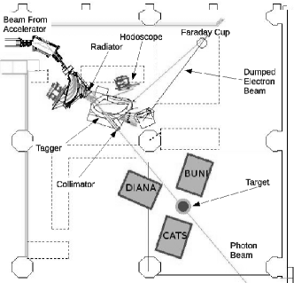
Figure 1: The layout of the experimental area showing the location of the tagging spectrometer, focal-plane hodoscope, deuterium target, and NaI(Tl) detectors labeled DIANA, BUNI, and CATS.

The tagging magnet and focal-plane (FP) hodoscope J.M. Vogt et al. (1993) were used extensively at the Saskatchewan Accelerator Laboratory prior to their use at the MAX IV Laboratory. The dipole field of the magnet is used to momentum analyze the post-bremsstrahlung electrons, which are detected in the FP hodoscope by 63 plastic scintillators. The scintillators are 25 mm wide and 3 mm thick and arranged into two rows. The rows are offset by 50% of the scintillator width, with each overlap defining a FP channel (see Fig. 2). The typical width of a FP channel was $\sim$400 keV and the nominal electron rate was 1 MHz/channel. As the Compton counting rate is low, the focal plane was subdivided into four bins. The central photon energies for each bin, as well as the average bin width, are given in Table 1.

Figure 2: Enlarged diagram of the tagger magnet and FP hodoscope portion of the experimental layout (not to scale).

The size of the photon beam was defined by a tapered tungsten-alloy primary collimator of 19 mm nominal diameter. The primary collimator was followed by a dipole magnet and a post-collimator which were used to remove any charged particles produced in the primary collimator. The beam spot at the target location was approximately 60 mm in diameter.

The tagging efficiency J.-O. Adler et al. (1997) is the ratio of the number of tagged photons which struck the target to the number of post-bremsstrahlung electrons which were registered by the associated FP channel. It depends on the collimator size and the electron-beam energy. It was measured during the experiment start-up with the three large-volume NaI(Tl) photon spectrometers placed directly in the low-intensity photon beam and was monitored during data collection on a daily basis via dedicated measurements with a compact lead-glass photon detector, which was easily raised into and lowered out of the photon beam.

The liquid deuterium target used in this experiment was based on a design used in previous measurements Lundin et al. (2003), but with measures developed to eliminate ice build-up on the target endcaps. These measures included a several-day bake-out of the vacuum vessel to reduce internal gases, thicker Kapton foils for the vacuum chamber windows, and the implementation of a N₂ gas shield. These last two measures reduce the penetration of water vapor from the air into the insulation vacuum surrounding the cell. The cell was cylindrical, 150 mm long and 68 mm in diameter. The spherical endcaps were convex so that the total length of the cell was 170 mm. The cell was oriented so that its central axis was collinear with the beam line. The housing chamber was constructed of stainless steel with a thickness of $\sim$1 mm in the vicinity of the scattering plane and $\sim$2 mm elsewhere.

Three large-volume, segmented NaI(Tl) detectors labeled BUNI J.P. Miller et al. (1988), CATS Wissmann et al. (1999), and DIANA L.S. Myers (2010) in Fig. 1 were used to detect the Compton-scattered photons. The detectors were located at laboratory angles of 60^∘, 120^∘, and 150^∘. These detectors were each composed of a NaI(Tl) core surrounded by optically isolated, annular NaI(Tl) segments. The cores of the BUNI and CATS detectors each measure 26.7 cm in diameter, while the core of the DIANA detector measures 48.0 cm. The depth of all three detectors is greater than 20 radiation lengths. The annular segments are 11 cm thick on the BUNI and CATS detectors and 4 cm thick on the DIANA detector. Additionally, BUNI and CATS each has a plastic-scintillator annulus that surrounds the NaI(Tl) annulus. Each detector was shielded by lead with a front aperture that defined the detector acceptance. A plastic-scintillator paddle was placed in front of the aperture to identify and veto charged particles. The detectors have an energy resolution of better than 2% at energies near 100 MeV. Such resolution is necessary to separate unambiguously the elastically scattered photons from those originating from the breakup of deuterium.

The signals from each detector were passed to analog-to-digital converters (ADCs) and time-to-digital converters (TDCs) and the data were recorded on an event-by-event basis. The experimental data were collected in two separate four-week run periods. The first run period employed an electron-beam energy of 144 MeV; the second run period used 165 MeV. The first week of each period was dedicated to in-beam studies (see below), measurements of ¹²C($\gamma$,$\gamma$) L.S. Myers et al. (2014c) to establish the absolute normalization and systematics of the setup, and cooling of the liquid-deuterium target. The remaining three weeks were used to perform the measurements on deuterium reported in this article.

III Data Analysis

The Compton scattering cross section can be written as

$$\frac{d\sigma}{d\Omega}=(\frac{Y}{\Omega_{\rm eff}})\frac{1}{N_{\gamma}}\frac{1}{\kappa_{\rm eff}}f_{\rm R}f_{\rm T},$$ (7)

where $(Y/\Omega_{\rm eff})$ is the scattered-photon yield normalized to the effective solid-angle acceptance of the detector, $N_{\gamma}$ is the number of tagged photons incident upon the target, and $\kappa_{\rm eff}$ is the effective thickness of the target (the number of nuclei per unit area). $f_{\rm R}$ and $f_{\rm T}$ represent correction factors due to rate- and target-dependent effects, respectively, as explained below.

III.1 Acceptance-normalized yield

III.1.1 Scattered-photon yield

During the experiment, the ADCs allowed reconstruction of the scattered-photon energies, while the TDCs enabled coincident timing between the NaI(Tl) detectors and the FP hodoscope. The energy calibration of each of the NaI(Tl) detectors was determined by placing it directly into the reduced-intensity photon beam and observing its response as a function of tagged-photon energy. To calibrate each ADC, a spectrum was filled (see the inset to Fig. 3) for each FP channel by selecting only on tagged photons for that channel. The position of the peak (in ADC channels) was then plotted against the expected photon energy, as determined from the tagging magnet field map, for all the FP channels. As an example, the calibration for BUNI is shown in Fig. 3.

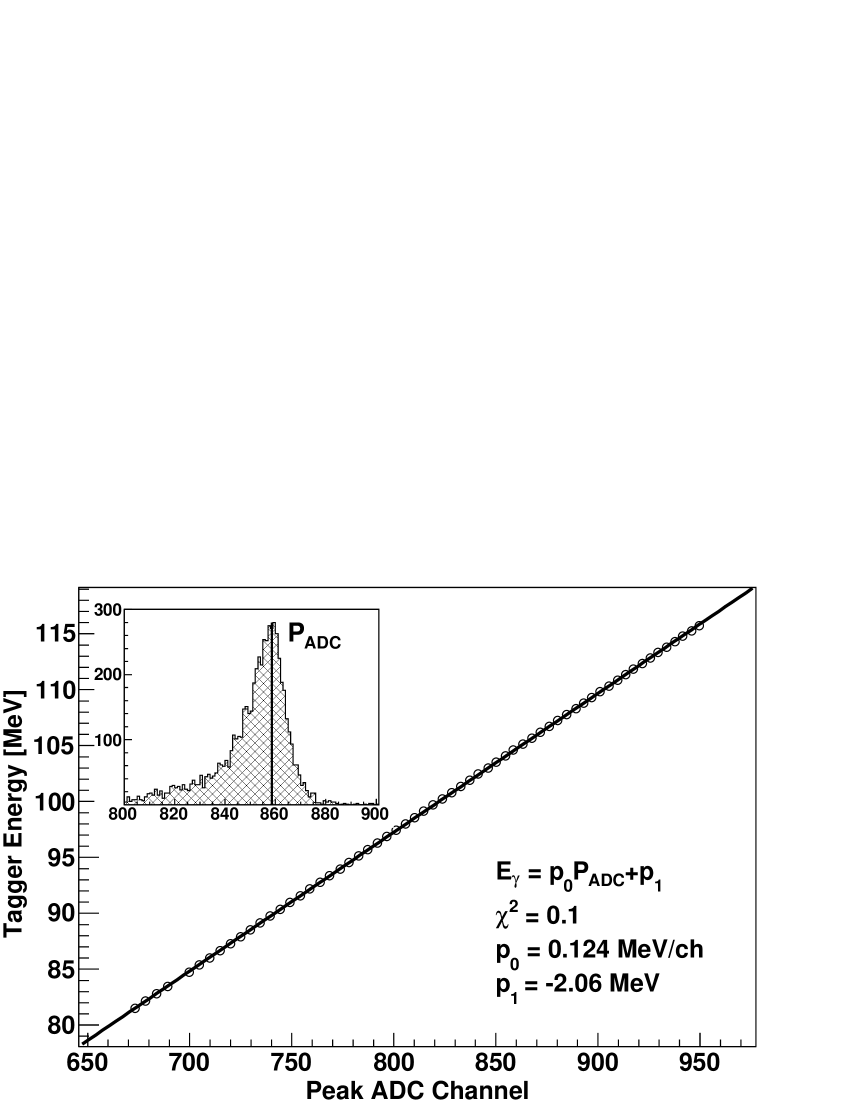
Figure 3: A plot of the predicted photon energy for each FP channel versus the peak position of the ADC spectrum (P_ADC) for the same channel. The plot is fit with a linear function to determine the calibration of the NaI(Tl) detector. (Inset) A typical tagged-photon ADC spectrum for BUNI showing the location of the ADC channel corresponding to the peak (P_ADC).

Missing energy (ME) was defined to be the difference between the expected energy of the detected photon (as determined from the tagger magnet and FP hodoscope placement) and the energy deposited by the photon in the NaI(Tl) detector. In both BUNI and CATS, the energy deposition in the annulus was added to the core energy deposition to improve the resolution. The measured in-beam response for the BUNI detector, together with a fitted GEANT4 Agostinelli (2003) simulation of this response, is shown in Fig. 4. The GEANT4 simulation output was determined for the case of the BUNI detector positioned directly in the photon beam. This “intrinsic” simulation was then smeared with a Gaussian function according to

$$\mathcal{R}_{i}^{\rm inbeam}=\sum\limits_{j}\frac{p_{\rm 1}}{E_{j}p_{\rm 3}}e^{\frac{(E_{i}-E_{j}-p_{\rm 2})^{2}}{-2(E_{j}p_{\rm 3})^{2}}}\mathcal{S}_{j}^{\rm inbeam},$$ (8)

where $E_{i\left(j\right)}$ was the central energy of bin $i$($j$), $\mathcal{S}_{j}^{\rm inbeam}$ was the number of counts in bin $j$ of the simulated detector-response spectrum, and $p_{\rm 1,2,3}$ were fitting parameters that accounted for the individual characteristics of each NaI(Tl) detector, such as non-uniform doping of the crystal, that are difficult to model in GEANT4. This process was repeated for CATS and DIANA.

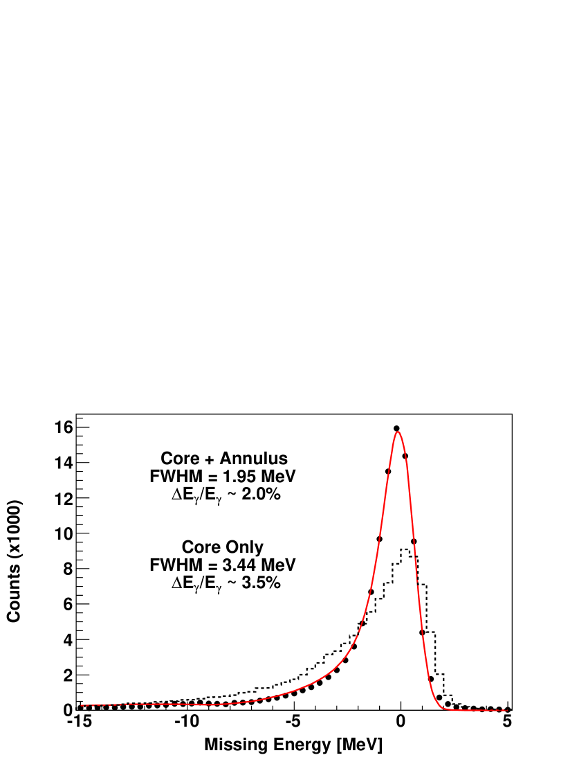
Figure 4: (Color online) In-beam detector response as a function of missing energy for the BUNI detector. The data points are the result of summing the energy deposition in both the NaI(Tl) core and annulus. The solid red curve is the simulated GEANT4 detector response fitted to the data. The dashed line is the ME spectrum obtained by analyzing only the core crystal. The addition of the annulus energy improves the FWHM by almost 50%.

It was observed that the gain of the NaI(Tl) detectors drifted over the course of the run periods. In order to correct for this gain drift, cosmic-ray data were collected immediately after each in-beam calibration run and prior to moving the detector to its scattering location. “Straight-through” cosmic rays, defined by requiring a large energy deposition in annular segments on opposite sides of the core crystal, were selected because these events should have a constant energy deposition in the detector. The gain drift for each PMT for each run could be determined by monitoring the location and shape of the resulting cosmic-ray peaks. These gain-drift corrections were then applied to the data.

The energy calibration of the tagger focal plane was confirmed by observing highly energetic capture photons from the $\pi^{-}+d\rightarrow\gamma+2n$ reaction. This reaction channel was present as the untagged bremssstrahlung spectrum extended beyond pion production threshold energy, and the most probable energy of the capture photon is $\sim$131 MeV Gabioud et al. (1979). The agreement between the absolute photon energy and that reconstructed from the tagger FP energy calibration was better than 1%.

Large backgrounds arose when the beam intensity was increased from 10-100 Hz per FP channel (for in-beam runs) to $\sim$1 MHz per channel (for scattering runs). The dominant sources of background were untagged bremsstrahlung photons (which scaled with the beam intensity) and cosmic rays. These backgrounds obscured the timing and ME peaks of the elastic photons in the TDC and ADC spectra, respectively. Cosmic rays deposit a large amount of energy in the detector overall and in the annular segments in particular. A cut placed on the NaI(Tl) annulus (BUNI and DIANA) or the plastic-scintillator (CATS) annulus removed $\sim$95% of the cosmic-ray background from the scattering data. An additional cut placed on the thin plastic-scintillator paddle in front of each of the NaI(Tl) detectors removed charged particles. These cuts reduced the number of events by $\sim$50%.

In order to further reduce the untagged bremsstrahlung background in the FP TDC spectrum, a cut was placed on the energy deposited in the NaI(Tl) detector. Selecting only events with an energy deposition $E_{\rm min}\leq E\leq E_{\rm max}$, where $E_{\rm min(max)}$ is the minimum (maximum) tagged-photon energy, enabled the prompt peak to be identified in the FP TDC spectrum (see Fig. 5). This prompt peak represented coincidences between post-bremsstrahlung electrons in the FP hodoscope and elastically scattered photons in the NaI(Tl) detectors.

For each NaI(Tl) detector and for each FP channel, events occurring within the prompt peak were selected and a prompt ME spectrum was filled. The process was repeated for a second cut placed on a purely accidental timing region, and an accidental spectrum was filled.

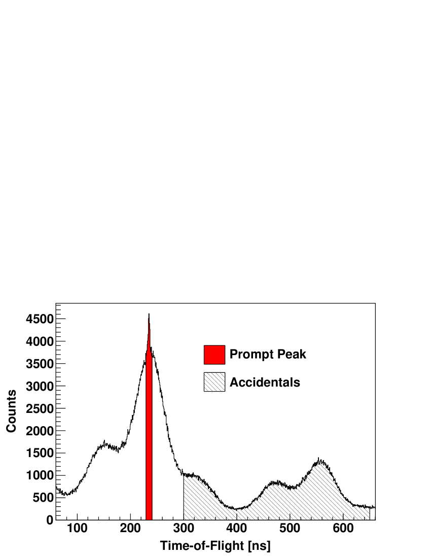
Figure 5: (Color online) The FP TDC spectrum for the scattering data. The prompt (red) and the accidental (shaded) windows are indicated.

For each run period, data collected during dedicated, beam-off cosmic-ray runs were utilized to remove the $\sim$5% of cosmic-ray events that survived the annulus cuts. For each NaI(Tl) detector and for each FP channel, these data were subjected to the same annulus cuts above, and cosmic-ray spectra were filled. These spectra were scaled by the ratio of events with an energy exceeding the electron-beam energy in the prompt spectra to those in the cosmic-ray spectra, and then subsequently subtracted from the prompt spectra. The procedure was repeated for the accidental spectra. In this way, prompt and accidental spectra free from cosmic rays were produced.

The GEANT4 in-beam simulation was extended to reflect the experimental setup for scattering runs. A numerical function $\mathcal{F}_{i}$ was defined by

$$\mathcal{F}_{i}=p_{\rm 0}\mathcal{A}_{i}+\mathcal{R}_{i}^{\rm scatter},$$ (9)

where $\mathcal{A}_{i}$ was the number of counts in bin $i$ of the accidental spectrum, $p_{\rm 0}$ was the scale factor of the accidentals, and $\mathcal{R}_{i}^{\rm scatter}$ was given by Eq. (8) using the scattering response spectrum from the GEANT4 simulation (see the top panel of Fig. 6). The range of the fitting window varied from as small as [–10,+10] MeV to as large as [–20,+20] MeV in ME. By fitting several windows over this range, an estimate of the dependence of the extracted yield on the width of the fitting window was obtained. This kinematic-dependent uncertainty depended strongly on the signal-to-noise ratio in the prompt ME spectrum and ranged from 2% to 11%.

The bottom panel of Fig. 6 shows a typical “true” scattering spectrum (prompts minus accidentals) together with the corresponding fitted, convoluted response function $\mathcal{R}_{i}^{\rm scatter}$. The scattering yield was extracted by integrating the true spectrum over the region of interest (ROI) ($-$2.0 MeV $\leq$ ME $\leq$ 2.0 MeV) indicated by the vertical dashed lines. The ROI was not allowed to extend below $-$2.0 MeV as photons from the photodissociation of the deuteron are kinematically allowed in this region. The elastically scattered photon yields determined according to this procedure are given in Table 2.

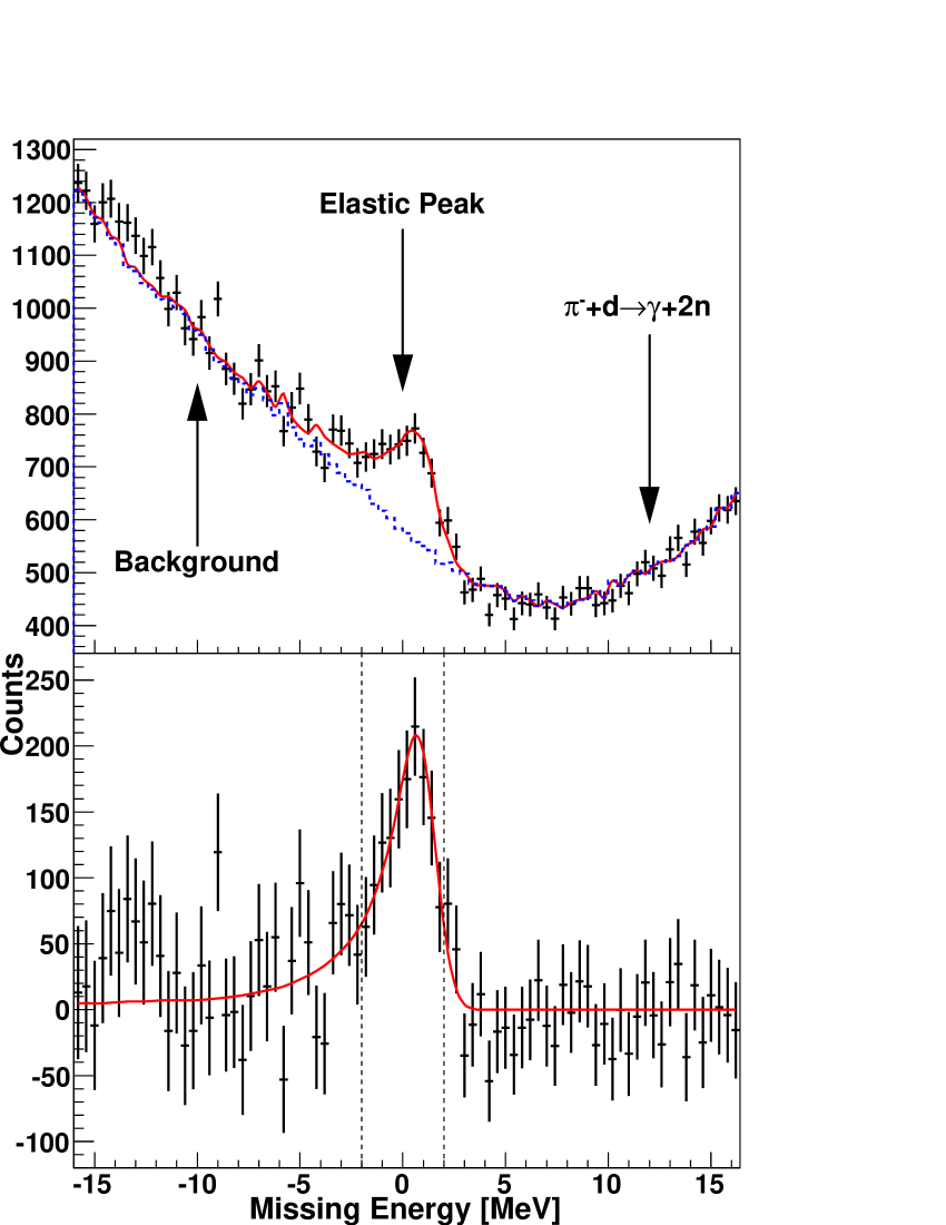
Figure 6: (Color online) Top panel: The result of fitting the sum (solid) of the accidental spectrum (dashed) and the fitted detector response to the prompt spectrum. Bottom panel: The true elastic peak (prompts minus accidentals) together with the fitted detector response (solid). The vertical, dashed lines indicate the region of integration over which the yield extraction occurs, $-$2.0 MeV $\leq$ ME $\leq$ 2.0 MeV.

The $-$2.0 MeV $\leq$ ME $\leq$ 2.0 MeV ROI was carefully chosen, taking into account the detector resolution (FWHM <2% at 100 MeV), to minimize the contribution of photons from $d$($\gamma$,$\gamma^{\prime}$)$n$$p$ to the extracted yield. Contamination from non-elastic photons was investigated with a direct and an indirect search. The direct method involved simulating the photons from the breakup reaction and adding this new lineshape to the fitting algorithm. This new lineshape was displaced 2.2 MeV to the low-energy side of the elastic peak to account for the reaction threshold. The data were re-fit and the contribution of the non-elastic photons to the extracted yield was calculated. This contribution was found to be consistent with zero within uncertainties. The indirect method relied on the quality of the fit shown in Fig. 6, which has a typical reduced $\chi^{2}$ value of $\lesssim$ 1. If there were a sizable contribution arising from a non-elastic reaction, it would cause the extracted cross sections to vary depending on the ROI width. Since non-elastic photons lie to the left of the elastic peak, the lower edge of the ROI was varied by $\pm$400 keV. It was found that the extracted cross sections with the varied ROIs agreed with the ones listed in this paper within uncertainties. Thus, it was concluded that the cross sections presented here do not suffer from contributions from $d$($\gamma$,$\gamma^{\prime}$)$n$$p$.

III.1.2 Detector Acceptance

The detector acceptances depended on the cuts employed during the data analysis and the width and location of the integration ROI. The geometrical solid angle subtended by the NaI(Tl) detectors was corrected for the geometry of the experimental setup. Both of these effects were studied using the GEANT4 Monte Carlo simulations. The effective solid angle $\Omega_{\rm eff}$ was given by

$$\Omega_{\rm eff}=\frac{N_{\rm events}^{\rm ROI}}{N_{\rm events}}~{}4\pi,$$ (10)

where $N_{\rm events}$ was the total number of simulated events, and $N_{\rm events}^{\rm ROI}$ was the number of simulated events that eventually populated the ROI.

The cosmic-rejection cuts removed a very small number of good Compton-scattered photons from the ROI. For the CATS (60^∘) detector, the plastic-scintillator annulus was used as a cosmic-ray veto. For the DIANA (150^∘) detector, the thin NaI(Tl) annulus was used to reject cosmic rays. In each case, the cosmic-ray veto was more than 20 cm from the central cylindrical symmetry axis of the detector and only $\sim$1% of all elastically scattered photons were rejected. For the BUNI (120^∘) detector, annular NaI(Tl) segments $\sim$13 cm from the cylindrical symmetry axis of the detector were used for the rejection of cosmic rays. As a result, 6% of all scattered photons were rejected. However, the NaI(Tl) segments in BUNI provided sufficient energy resolution to determine the cut placement accurately resulting in a systematic uncertainty of $\sim$2%. The charged-particle veto removed $\sim$1% of all scattered photons.

The effective solid angle for each data point is given in Table 2. A sufficient number of events were simulated so that the statistical uncertainties are $\leq$1%. The systematic uncertainties include the effects of the cosmic-rejection cuts as well as uncertainty from measurements of the target-detector distance and detector-aperture diameter, typically $\pm$2 mm.

Table 2: Extracted yields and effective solid angle at each energy and angle. For the yields, the first uncertainty is statistical and the second is a kinematic-dependent systematic. For the effective solid angles, the first uncertainty is statistical and the second is an angle-dependent systematic. The upper four energy bins are from RP1 and the lower four from RP2 (also in Tables 3, 4, and 6).

$E_{\gamma}$	60∘		120∘		150∘
(MeV)	$Y$	$\Omega_{\rm eff}$ (msr)	$Y$	$\Omega_{\rm eff}$ (msr)	$Y$	$\Omega_{\rm eff}$ (msr)
69.6	1080 $\pm$ 182 $\pm$ 61	29.0 $\pm$ 0.3 $\pm$ 1.2	1106 $\pm$ 191 $\pm$ 42	42.9 $\pm$ 0.4 $\pm$ 1.9
77.9	995 $\pm$ 137 $\pm$ 59	25.3 $\pm$ 0.3 $\pm$ 1.1	1528 $\pm$ 152 $\pm$ 32	42.9 $\pm$ 0.4 $\pm$ 1.9	1034 $\pm$ 142 $\pm$ 84	22.8 $\pm$ 0.2 $\pm$ 0.7
86.1	809 $\pm$ 93 $\pm$ 18	28.1 $\pm$ 0.3 $\pm$ 1.2	1312 $\pm$ 115 $\pm$ 26	38.1 $\pm$ 0.4 $\pm$ 1.6	790 $\pm$ 115 $\pm$ 41	22.6 $\pm$ 0.2 $\pm$ 0.7
93.4	440 $\pm$ 63 $\pm$ 13	26.5 $\pm$ 0.3 $\pm$ 1.1	1148 $\pm$ 90 $\pm$ 23	38.2 $\pm$ 0.4 $\pm$ 1.6	573 $\pm$ 90 $\pm$ 63	22.2 $\pm$ 0.2 $\pm$ 0.7
85.8	1669 $\pm$ 199 $\pm$ 187	24.0 $\pm$ 0.2 $\pm$ 1.0	2199 $\pm$ 156 $\pm$ 187	41.6 $\pm$ 0.4 $\pm$ 1.8	1616 $\pm$ 198 $\pm$ 50	20.2 $\pm$ 0.2 $\pm$ 0.6
94.8	1639 $\pm$ 161 $\pm$ 127	18.9 $\pm$ 0.2 $\pm$ 0.8	2633 $\pm$ 142 $\pm$ 94	41.1 $\pm$ 0.4 $\pm$ 1.8	1587 $\pm$ 174 $\pm$ 48	19.8 $\pm$ 0.2 $\pm$ 0.6
103.8	1266 $\pm$ 117 $\pm$ 30	21.0 $\pm$ 0.2 $\pm$ 0.9	1919 $\pm$ 117 $\pm$ 55	39.2 $\pm$ 0.4 $\pm$ 1.7	1424 $\pm$ 141 $\pm$ 71	19.3 $\pm$ 0.2 $\pm$ 0.6
112.1	842 $\pm$ 91 $\pm$ 21	21.5 $\pm$ 0.2 $\pm$ 0.9	1370 $\pm$ 95 $\pm$ 29	37.7 $\pm$ 0.4 $\pm$ 1.6	1034 $\pm$ 115 $\pm$ 29	19.4 $\pm$ 0.2 $\pm$ 0.6

III.2 Scale normalization

III.2.1 Number of beam photons

The number of beam photons incident on the target $N_{\gamma}$ was determined from

$$N_{\gamma}=N_{e}\cdot\varepsilon_{\rm tag},$$ (11)

where $N_{e}$ is the number of post-bremsstrahlung electrons detected in each FP channel and $\varepsilon_{\rm tag}$ is the tagging efficiency.

The number of electrons striking the focal plane ($N_{e}$) was counted by the FP scalers (see Table 3). The background rate in the focal plane, obtained from beam-off runs, was on the order of 1 Hz per channel and was thus negligible compared to the beam-on electron rate of $\sim$1 MHz per channel. The tagging efficiency $\varepsilon_{\rm tag}$ was determined from the ratio of the number of photons tagged by a FP channel and recorded in the in-beam photon detector to the number of post-bremsstrahlung electrons recorded by the same channel. Livetime-corrected beam-on and beam-off backgrounds ($\sim$5%) were removed from the data. The focal plane was divided into four bins, each 16 channels wide. The tagging efficiency for each bin was taken to be the electron-weighted average of the tagging efficiencies for each of the 16 channels. A plot of the daily tagging efficiency measured using the compact lead-glass detector for the $E_{\gamma}$ = 93.4 MeV bin is shown in Fig. 7.

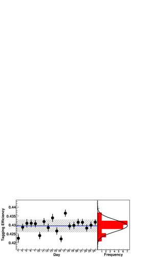
Figure 7: Time evolution of the tagging efficiency measured using the compact lead-glass detector for the $E_{\gamma}$ = 93.4 MeV bin from RP1. The shaded region indicates the uncertainty due to daily variations in $\varepsilon_{\rm tag}$.

In order to observe any systematic difference between the tagging efficiency determined by the NaI(Tl) detectors and the lead-glass detector, measurements were taken with the CATS detector and immediately thereafter with the lead-glass detector. These data allowed for a <2% correction to be made to the compact lead-glass detector results, mainly due to the larger volume of the NaI(Tl) and the presence of the thin paddle used to veto charged particles. This correction was applied to the average value of the tagging efficiency determined with the compact lead-glass detector. One-half of the correction was assigned as a systematic uncertainty.

The number of post-bremsstrahlung electrons $N_{e}$, tagging efficiencies $\varepsilon_{\rm tag}$, and number of beam photons $N_{\gamma}$ are presented in Table 3.

Table 3: Number of post-bremsstrahlung electrons, tagging efficiencies, and number of tagged photons. The relative statistical and systematic uncertainties of $N_{\gamma}$ are the same as those for $\varepsilon_{\rm tag}$. The upper four energy bins are from RP1 and the lower four from RP2.

$E_{\gamma}$	$N_{e}$ ($\times$ 1013)	$\varepsilon_{\rm tag}$	$\delta\varepsilon_{\rm tag}$	$\delta\varepsilon_{\rm tag}$	$N_{\gamma}$ ($\times$ 1012)
(MeV)	[60∘, 120∘, 150∘]		(statistical)	(systematic)	[60∘, 120∘, 150∘]
69.6	1.06, 1.06, 1.05	0.421	0.002	0.005	4.47, 4.47, 4.43
77.9	1.12, 1.12, 1.11	0.423	0.002	0.005	4.73, 4.73, 4.69
86.1	0.941, 0.941, 0.931	0.426	0.002	0.005	4.01, 4.01, 3.97
93.4	0.782, 0.782, 0.775	0.425	0.002	0.005	3.32, 3.32, 3.29
85.8	1.72, 1.72, 1.71	0.456	0.004	0.007	7.83, 7.83, 7.79
94.8	1.85, 1.85, 1.84	0.459	0.004	0.008	8.50, 8.50, 8.45
103.8	1.58, 1.58, 1.57	0.460	0.004	0.008	7.26, 7.26, 7.22
112.1	1.37, 1.37, 1.36	0.458	0.005	0.008	6.24, 6.24, 6.21

III.2.2 Effective target thickness

The effective target thickness $\kappa_{\rm eff}$ (the number of nuclei per unit area) was given by

$$\kappa_{\rm eff}=\frac{\rho~{}L~{}N_{A}}{A},$$ (12)

where $\rho$ was the average density of liquid deuterium, $L$ was the effective target length, $N_{A}$ was Avogadro’s number, and $A$ was the molar mass (4.0282 g/mol).

The target pressure and temperature were systematically recorded for each run. As the density of liquid deuterium is related to its pressure T. Glebe (1993), an average target density was calculated by determining the deuterium density measured during each run and weighting this density by the number of FP electrons recorded in the same run. For each run period, the average density of the liquid deuterium in the target cell was thus determined to be $\rho$ = (0.163 $\pm$ 0.002) g/cm³.

The cylindrical portion of the liquid deuterium target cell measured 68 mm in diameter and 150 mm in length. The convex endcaps each added an additional 10 mm to the cell length at the central symmetry axis (which also corresponded to the photon-beam axis). Thus, the total length of the liquid deuterium target cell along its symmetry axis was 170 mm. Due to the cell geometry and the divergent nature of the photon trajectories originating from the radiator, the target thickness for each individual photon trajectory differed from this measured target length along the symmetry axis. A Monte Carlo simulation was thus employed to determine the effective target length for an “average” beam photon. The angular distribution of the photons emanating from the radiator was determined from a series of tagging-efficiency measurements taken with photon-beam collimators of different diameters.

The effective target length was determined to be $L$ = (166 $\pm$ 2) mm. $\kappa_{\rm eff}$ was thus determined to be (8.10 $\pm$ 0.20) $\times$ 10²³ (nuclei/cm²), where the systematic uncertainty is the sum, in quadrature, of the uncertainties in $\rho$ and $L$ together with an additional 2% uncertainty to account for any potential misalignment of the symmetry axis of the target relative to the trajectory of the photon beam.

III.3 Corrections

III.3.1 Rate-dependent Corrections

The rate-dependent correction arises from high electron rates producing dead time in the single-hit FP TDCs and scalers. The nominal average electron rate of 1 MHz per FP channel, but the instantaneous rate fluctuated markedly and was as large as 4 MHz. The origins of these effects has been presented in detail in Ref. L.S. Myers et al. (2013), where a description of the Monte Carlo simulation of the FP electronics used to quantify the effects is also presented. We note that this procedure has been used to successfully extract Compton scattering cross sections from carbon – see Refs. L.S. Myers et al. (2014c); M.F. Preston et al. (2014). A short summary is presented below.

The rate-dependent correction was the product of three terms

$$f_{\rm R}=f_{\rm ghost}f_{\rm stolen}f_{\rm missed},$$ (13)

where $f_{\rm ghost}$ was the correction arising from accidental coincidences between the front and back scintillator planes in the FP hodoscope, $f_{\rm stolen}$ corrected for prompt electrons that are not observed in the prompt peak because an accidental electron stopped the single-hit TDC previously, and $f_{\rm missed}$ accounted for prompt electrons missed by the FP TDC but not the FP scaler due to deadtime in the electronics. Typical values for $f_{\rm ghost}$ and $f_{\rm missed}$ were 5% and 1% respectively, while $f_{\rm stolen}$ ranged from 15 – 50% depending upon the FP rate for the runs in question. A summary of the values of the rate-dependent correction $f_{\rm R}$ is presented in Table 4, where the first uncertainty is a scale systematic uncertainty common to all data points and the second is a kinematic-dependent systematic uncertainty that arises uniquely from $f_{\rm stolen}$.

III.3.2 Target-related Corrections

The target-related correction was given by

$$f_{\rm T}=f_{\rm abs}f_{\rm fill}f_{\rm cell},$$ (14)

where $f_{\rm abs}$ was due to the absorption of beam photons by the liquid deuterium prior to scattering, $f_{\rm fill}$ was due to incomplete filling of the target cell, and $f_{\rm cell}$ was due to beam photons scattering from the Kapton endcaps of the target cell. The absorption of beam photons by the liquid deuterium prior to scattering was determined using a GEANT4 Monte Carlo which considered the effective target thickness discussed in Sect III.2. The correction $f_{\rm abs}$ was determined to be $\sim$1.6%, and was known to better than 3% relative uncertainty.

During RP1, the liquid deuterium target did not fill completely. The liquid-deuterium level was observed each day by taking Polaroid images of the target cell which clearly showed the filled portion of the cell. Based on these images, it was determined that the top $\sim$1.6 cm of the target cell was unfilled. In order to account for beam photons that passed through this unfilled portion of the target, a Monte Carlo simulation similar to the one used to determine $\kappa_{\rm eff}$ was employed. The fraction of beam photons that struck the filled portion of the target was determined, taking into account both the angular divergence of the beam photons and the uncertainty in the observed target-fill line. The correction $f_{\rm fill}$ was determined to be 7%, and was known to better than 2.5% relative uncertainty.

The contribution of the thin Kapton endcaps to the scattered-photon yield was investigated using a $\sim$1 cm thick Kapton target. These Kapton data were subjected to the analysis detailed in Section III.1 to extract the thick Kapton target yield $Y_{\rm Kapton}$. The resulting correction to the scattered-photon yield due to the thin Kapton endcaps was given by

$$f_{\rm cell}=\frac{Y-xY_{\rm Kapton}}{Y},$$ (15)

where $x$ was a factor used to scale the thick Kapton target yield to the thin Kapton endcap yield. This scaling factor depended on the relative Kapton thicknesses, numbers of incident photons, and target geometries which affected detector acceptances. The correction factors for DIANA (150^∘) and BUNI (120^∘) were consistent with unity within uncertainties. The average correction factor or CATS (60^∘) was 94%. A systematic uncertainty of 2% in $f_{\rm cell}$ was determined for each detector. The target-related corrections are given in Table 4.

Table 4: Rate- and target-dependent corrections. The first uncertainty in $f_{\rm R}$ is a systematic that is common to all data points, while the second uncertainty is a kinematic-dependent systematic. The uncertainties in $f_{\rm T}$ are systematic. The upper four energy bins are from RP1 and the lower four from RP2.

$E_{\gamma}$	60∘		120∘		150∘
(MeV)	$f_{\rm R}$	$f_{\rm T}$	$f_{\rm R}$	$f_{\rm T}$	$f_{\rm R}$	$f_{\rm T}$
69.6	1.49 $\pm$ 0.05 $\pm$ 0.03	1.03 $\pm$ 0.03	1.60 $\pm$ 0.05 $\pm$ 0.02	1.09 $\pm$ 0.04	1.49 $\pm$ 0.05 $\pm$ 0.04	1.09 $\pm$ 0.04
77.9	1.40 $\pm$ 0.04 $\pm$ 0.03	1.03 $\pm$ 0.03	1.49 $\pm$ 0.05 $\pm$ 0.02	1.09 $\pm$ 0.04	1.42 $\pm$ 0.04 $\pm$ 0.03	1.09 $\pm$ 0.04
86.1	1.31 $\pm$ 0.04 $\pm$ 0.02	1.02 $\pm$ 0.03	1.36 $\pm$ 0.04 $\pm$ 0.01	1.09 $\pm$ 0.04	1.33 $\pm$ 0.04 $\pm$ 0.02	1.09 $\pm$ 0.04
93.4	1.28 $\pm$ 0.04 $\pm$ 0.02	1.02 $\pm$ 0.03	1.32 $\pm$ 0.04 $\pm$ 0.01	1.09 $\pm$ 0.04	1.30 $\pm$ 0.04 $\pm$ 0.02	1.09 $\pm$ 0.04
85.8	1.30 $\pm$ 0.04 $\pm$ 0.01	0.96 $\pm$ 0.02	1.58 $\pm$ 0.05 $\pm$ 0.02	1.02 $\pm$ 0.02	1.30 $\pm$ 0.04 $\pm$ 0.02	1.02 $\pm$ 0.02
94.8	1.26 $\pm$ 0.04 $\pm$ 0.01	0.96 $\pm$ 0.02	1.48 $\pm$ 0.05 $\pm$ 0.01	1.02 $\pm$ 0.02	1.26 $\pm$ 0.04 $\pm$ 0.02	1.02 $\pm$ 0.02
103.8	1.21 $\pm$ 0.04 $\pm$ 0.01	0.96 $\pm$ 0.02	1.39 $\pm$ 0.04 $\pm$ 0.01	1.02 $\pm$ 0.02	1.22 $\pm$ 0.04 $\pm$ 0.01	1.02 $\pm$ 0.02
112.1	1.19 $\pm$ 0.04 $\pm$ 0.01	0.96 $\pm$ 0.02	1.34 $\pm$ 0.04 $\pm$ 0.01	1.02 $\pm$ 0.02	1.20 $\pm$ 0.04 $\pm$ 0.01	1.02 $\pm$ 0.02

III.4 Uncertainties

The dominant contribution to the statistical uncertainty came from the yield. The systematic uncertainties were divided into three classes: scale, angle-dependent, and kinematic-dependent. Scale uncertainties affected the data obtained at all angles and energies in a given run period equally. Angle-dependent uncertainties affected the results from the individual detectors differently. Kinematic-dependent uncertainties affected each measured data point individually. We report these uncertainties separately. The sources of systematic uncertainties are listed in Table 5 along with typical values.

Table 5: Sources and magnitudes of systematic uncertainties for the two run periods.

Type	Source	RP1	RP2
Scale	Tagging Efficiency	1.1%	1.6%
	Target Thickness	2.5%	2.5%
	Missed Trues	1.5%	1.5%
	Stolen Trues	1.0%	1.0%
	Ghost Events	2.4%	2.4%
	Kapton Cell	2.0%	2.0%
	Target Fill Level	2.5%	N/A
Total		5.2%	4.7%
Other uncertainties
	Statistical	8–17%	5–12%
Angular	Detector Acceptance	3–4%	3–4%
Kinematic	Yield Extraction	2–11%	2–11%
	Stolen Trues	1–3%	1–3%

IV Results

IV.1 Cross Sections

With the data analyzed as described above, we present the central result of our experiment in Table 6: elastic Compton scattering cross sections on the deuteron. The results are also shown in Fig. 8, along with those results at 66 MeV from Refs. M.A. Lucas (1994); Lundin et al. (2003) and 94 MeV from Ref. D.L. Hornidge et al. (2000) whose scattering angles are within $10^{\circ}$ of ours. Statistical uncertainties only are shown on the data points.

Table 6: Measured cross sections for deuteron Compton scattering at the lab angles listed. The first uncertainty is statistical, the second is the overall normalization (5.2% first run period, 4.7% second), the third is due to detector acceptance, and the last is kinematic-dependent. The upper four energy bins are from RP1 and the lower four from RP2.

$E_{\gamma}$	$\frac{d\sigma}{d\Omega}(60^{\circ})$	$\frac{d\sigma}{d\Omega}(120^{\circ})$	$\frac{d\sigma}{d\Omega}(150^{\circ})$
(MeV)	(nb/sr)	(nb/sr)	(nb/sr)
69.6	15.7 $\pm$ 2.6 $\pm$ 0.8 $\pm$ 0.7 $\pm$ 1.0	12.4 $\pm$ 2.2 $\pm$ 0.6 $\pm$ 0.5 $\pm$ 0.8	————
77.9	14.7 $\pm$ 2.0 $\pm$ 0.8 $\pm$ 0.6 $\pm$ 0.9	15.0 $\pm$ 1.3 $\pm$ 0.8 $\pm$ 0.6 $\pm$ 0.3	18.4 $\pm$ 2.5 $\pm$ 1.0 $\pm$ 0.6 $\pm$ 1.5
86.1	11.9 $\pm$ 1.4 $\pm$ 0.6 $\pm$ 0.5 $\pm$ 0.3	15.7 $\pm$ 1.4 $\pm$ 0.8 $\pm$ 0.7 $\pm$ 0.3	15.7 $\pm$ 2.3 $\pm$ 0.8 $\pm$ 0.5 $\pm$ 0.8
93.4	8.1 $\pm$ 1.2 $\pm$ 0.4 $\pm$ 0.3 $\pm$ 0.3	16.0 $\pm$ 1.3 $\pm$ 0.8 $\pm$ 0.7 $\pm$ 0.4	13.7 $\pm$ 2.2 $\pm$ 0.7 $\pm$ 0.4 $\pm$ 1.5
85.8	13.8 $\pm$ 1.7 $\pm$ 0.6 $\pm$ 0.6 $\pm$ 1.5	13.4 $\pm$ 1.0 $\pm$ 0.6 $\pm$ 0.6 $\pm$ 1.2	16.8 $\pm$ 2.0 $\pm$ 0.8 $\pm$ 0.5 $\pm$ 0.7
94.8	15.4 $\pm$ 1.5 $\pm$ 0.7 $\pm$ 0.7 $\pm$ 1.2	14.1 $\pm$ 0.8 $\pm$ 0.7 $\pm$ 0.6 $\pm$ 0.5	15.1 $\pm$ 1.7 $\pm$ 0.7 $\pm$ 0.5 $\pm$ 0.5
103.8	11.9 $\pm$ 1.1 $\pm$ 0.6 $\pm$ 0.5 $\pm$ 0.3	11.8 $\pm$ 0.7 $\pm$ 0.6 $\pm$ 0.5 $\pm$ 0.4	15.7 $\pm$ 1.6 $\pm$ 0.7 $\pm$ 0.5 $\pm$ 0.8
112.1	8.8 $\pm$ 1.0 $\pm$ 0.4 $\pm$ 0.4 $\pm$ 0.2	9.8 $\pm$ 0.7 $\pm$ 0.5 $\pm$ 0.4 $\pm$ 0.2	13.0 $\pm$ 1.5 $\pm$ 0.6 $\pm$ 0.4 $\pm$ 0.4

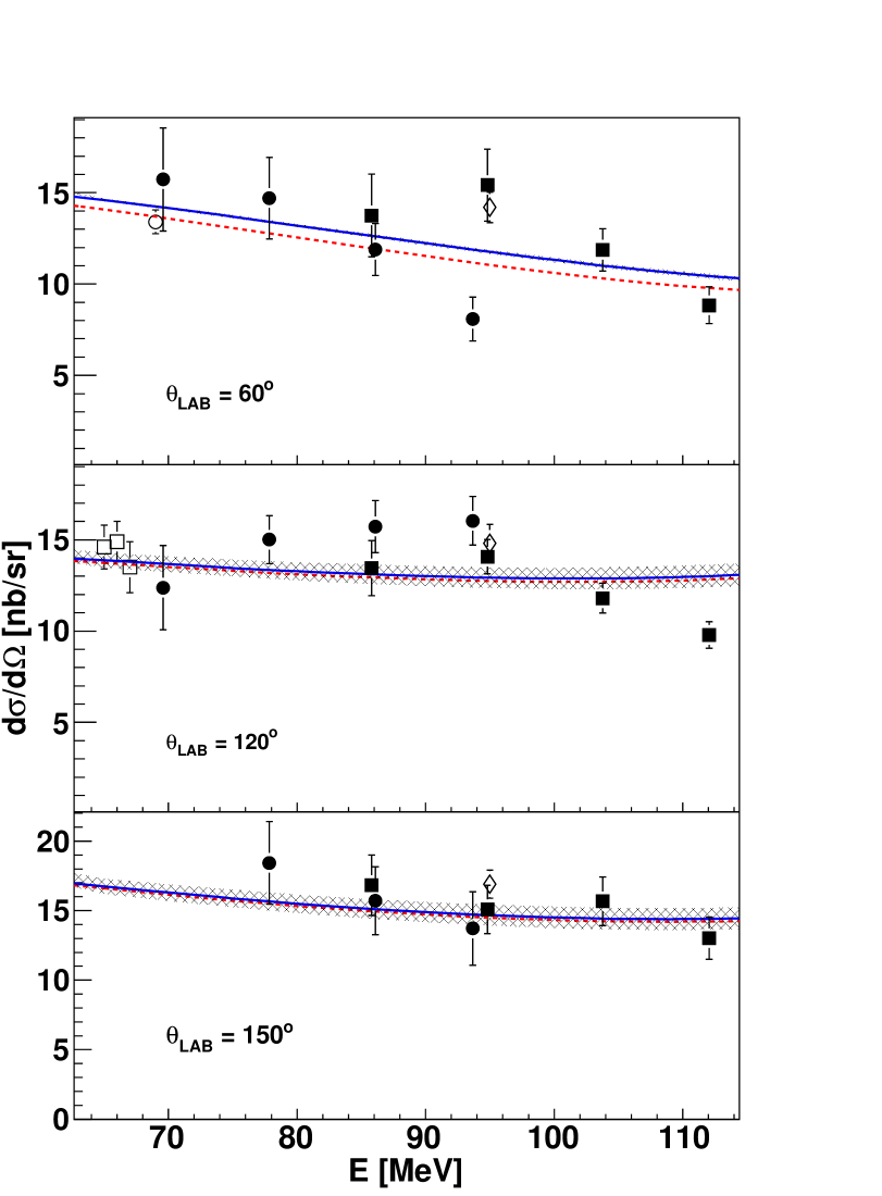
Figure 8: (Color online) Measurements of the deuteron Compton-scattering cross section from the current experiment (RP1 [$\bullet$] and RP2 [$\blacksquare$]) are shown. Previous measurements from References M.A. Lucas (1994) ($\circ$), Lundin et al. (2003) ($\Box$), and D.L. Hornidge et al. (2000) ($\diamond$) are included for comparison. Statistical uncertainties only are shown. The solid and dashed lines represent the free and BSR-constrained fits to the present data only. The shaded region is obtained by varying the BSR-constrained fit for $\alpha_{s}$ and $\beta_{s}$ by its statistical uncertainty.

The current world data set of deuteron Compton scattering cross sections is comprised of three measurements D.L. Hornidge et al. (2000); M.A. Lucas (1994); Lundin et al. (2003). The data reported here have uncertainties comparable to the previous data at low energies (E $\leq$ 70 MeV) and energy-bin widths considerably smaller than the previous high-energy (E = 95 MeV) measurement (Table 7). This experiment has doubled the number of data points in the world data set, in addition to providing the first data above 100 MeV. As Fig. 8 indicates, all data sets are in excellent agreement within their respective statistical uncertainties. This is corroborated by a complementing angle transect at $66$ and $94.5$ MeV, where these preceding measurements provide additional data beyond our scattering angles; see Ref. L.S. Myers et al. (2014a) for plots. Data consistency in the overlap is already a strong indication that our results can well be embedded into the consistent world data set, extending it to higher energies.

Table 7: Comparison of reported results from measurements of deuteron Compton scattering.

Ref.	E	$\Delta$E	Number	Normalization
	(MeV)	(MeV)	of Points	Uncertainty
M.A. Lucas (1994)	49,69	6.5,7.7	6	4%
D.L. Hornidge et al. (2000)	95	21	5	5–6%
Lundin et al. (2003)	55,67	10	18	6–14%
This work	70-112	7.3-9.0	23	5%

The figures also point to issues with two of our new data. The two points around $94.5$ MeV and $60^{\circ}$ are separated by $\sim$3$\sigma$, with the one from RP2 well in agreement with a SAL measurement and better agreeing with the overall trend. Another, more subtle, compatibility issue with the $(112.1$ MeV$,120^{\circ})$ point of the second run arises when comparing the data to fits, see also Refs. L.S. Myers et al. (2014a); fut . For both instances, the discrepancies could not be traced back to specific data or analysis issues. We therefore report these points but flag them as potential outliers, presenting results with them included in our extraction of the isoscalar nucleon polarizabilities in this paper.

IV.2 Nucleon Polarizabilities

As argued in the Introduction, the goal of this experiment was to provide new, high-quality data in support of an extraction of the neutron polarizabilities. Such a determination of these two-photon response parameters needs theoretical input, but it will also allow for a better understanding of the quality of our data.

First, the effects of nuclear binding and charged meson-exchange currents inside the deuteron must be subtracted. They contribute a significant fraction of the deuteron cross section at the energies we measured Beane et al. (1999), as well as in the zero-energy limit in which $\alpha_{E1}$ and $\beta_{M1}$ are defined Hildebrandt et al. (2010). For the individual amplitudes, one then needs to subtract the Powell amplitudes of point-like spin-$\nicefrac{{1}}{{2}}$ particles with anomalous magnetic moments.

More importantly, however, the nonzero-energy data must be related to the static point. In a simplistic extrapolation, one may be tempted to use a cross-section fit which identifies the electric and magnetic polarizabilities as angle-dependent contributions to the terms quadratic in the photon energy. This is, however, not permissible since all of our new data, and most of the world data, are well beyond its realm of applicability. At energies at and above $100$ MeV, the energy-dependent effects of the pion cloud and of the $\Delta(1232)$ excitation are important, and the pion-production threshold induces the first non-analyticity in the single-nucleon amplitudes. A low-energy expansion proceeds thus in powers of $\omega/m_{\pi}$ and becomes quickly useless.

A viable low-energy parametrization should hence consistently account for all these effects and provide a systematically improvable estimate of residual uncertainties. Chiral Effective Field Theory ($\chi$EFT) is ideally suited for this task. It model-independently encodes the correct symmetries and effective degrees of freedom of low-energy QCD, with a small dimensionless parameter to systematically improve the description of higher-order effects. It is well established that $\chi$EFT predicts the energy dependence of the single-nucleon Compton scattering response over the full range of data with high accuracy, including spin effects H.W. Grießhammer et al. (2012), and that it consistently accounts for nuclear binding as well as meson-exchange and nucleon-nucleon rescattering effects. All these aspects are necessary to restore the Thomson limit on the deuteron.

We therefore turn to the $\chi$EFT description which was used in previous high-accuracy descriptions of proton and deuteron Compton scattering. As its ingredients at next-to-leading order in $\alpha_{E1}$ and $\beta_{M1}$ (order $e^{2}\delta^{3}$) have recently been described summarily, we refer to Sect. 5.3 of Ref. H.W. Grießhammer et al. (2012) for details. The interactions between nucleons, pions and the $\Delta(1232)$ resonance are fully determined except for the two which parametrize short-distance contributions to the scalar polarizabilities. The dependence of the resulting extraction of $\alpha$ and $\beta$ on the deuteron wave function and $NN$ potential was shown to be negligible, and residual theoretical uncertainties were estimated as $\pm 0.8$ canonical units. In the results reported here, we use the same fit procedure and parameters as reported in Ref. H.W. Grießhammer et al. (2012). As described there, we add kinematic-dependent and angle-dependent systematic uncertainties in quadrature to the statistical uncertainty, and treat correlated overall systematic uncertainties by a floating normalization. This determination is based on the entire data set of our experiment, but does not include the other world data. Finally, we treat the two run periods as statistically independent data sets. Treating them as a single data set changes the following conclusions at most marginally.

Table 8 summarizes the findings of our fit, in the context of the previous extraction of the polarizabilities and the determination based on the new world data set which includes our data but with the two points previously mentioned discarded – these results being already reported in Ref. L.S. Myers et al. (2014a) and Eq. (6). For our extraction, as for the others, the values of the independent fit to $\alpha_{s}$ and $\beta_{s}$ demonstrate excellent consistency of $\alpha_{s}+\beta_{s}$ with the isoscalar BSR, Eq. (3). The BSR can therefore be used to reduce the number of parameters from two to one, decreasing the statistical uncertainties. In the fit to only the new data, the normalization of RP1 floats by about $2$% down, and that of RP2 by $3.5$% up, i.e. well within the overall correlated uncertainty. The statistical uncertainties are smaller than for the previous world data set, but the $\chi^{2}$ per degree of freedom is larger. As hinted above, this can be attributed to two points which between themselves contribute about $20$ units to $\chi^{2}$, while changing the central values only within the statistical uncertainties. A complementary publication fut provides details in the context of the construction of a consistent database. Here, we reiterate that a careful analysis of our data-taking and analysis procedures showed no intrinsic experimental reason why these points should be special.

Table 8: Isoscalar nucleon polarizabilities and $\chi^{2}$ per degree of freedom extracted from the world elastic deuteron Compton scattering data set prior to our data, from our data, and from the new world data set including our data, each using both a “free” fit to $\alpha_{s}$ and $\beta_{s}$ and a determination constrained by the BSR. Uncertainties are statistical only and anticorrelated for the BSR-constrained fits.

set	constraint	$\alpha_{s}$	$\beta_{s}$	$\chi^{2}$/d.o.f	Ref.
old world	free	$10.5\pm 2.0$	$3.6\pm 1.0$	$24.3/24$
	BSR	$10.9\pm 0.9$	$3.6\mp 0.9$	$24.3/25$	H.W. Grießhammer et al. (2012)
this work	free	$13.2\pm 1.4$	$3.2\pm 1.1$	$40.6/19$
	BSR	$12.1\pm 0.8$	$2.4\mp 0.8$	$41.7/20$
new world	free	$11.1\pm 0.9$	$3.3\pm 0.6$	$49.2/43$
	BSR	$11.1\pm 0.6$	$3.4\mp 0.6$	$45.2/44$	L.S. Myers et al. (2014a)

Our central values for either fit agree with those of the old and new world database extractions well within the systematic uncertainties only, not accounting for theoretical and BSR uncertainties. Since it effectively doubles the world data, it is therefore no surprise that the new world average reported in Ref. L.S. Myers et al. (2014a) is hardly shifted but its statistical uncertainty is reduced to $1/\sqrt{2}\approx 70\%$ of the previous one.

With only our current data, we thus obtain the final values of the BSR-constrained fit as

$$\begin{split}&\alpha_{s}=12.1\pm 0.8(\text{stat})\pm 0.2(\text{BSR})\pm 0.8(\text{th})\\ &\beta_{s}=2.4\mp 0.8(\text{stat})\pm 0.2(\text{BSR})\mp 0.8(\text{th}),\end{split}$$ (16)

where the uncertainties from theory and from the BSR constraint are listed separately. One finally extracts the neutron polarizabilities by combining with the proton values of Eq. (1) which were determined using the same $\chi$EFT approach and fit philosophy

$$\begin{split}&\alpha_{n}=13.55\pm 1.6(\text{stat})\pm 0.2(\text{BSR})\pm 0.8(\text{th})\\ &\beta_{n}=1.65\mp 1.6(\text{stat})\pm 0.2(\text{BSR})\mp 0.8(\text{th}).\end{split}$$ (17)

We list these values for completeness only, since those obtained from the new, statistically consistent world data set L.S. Myers et al. (2014a) supersede them in accuracy

$$\begin{split}&\alpha_{n}=11.55\pm 1.25(\text{stat})\pm 0.2(\text{BSR})\pm 0.8(\text{th})\\ &\beta_{n}=3.65\mp 1.25(\text{stat})\pm 0.2(\text{BSR})\mp 0.8(\text{th}).\end{split}$$ (18)

In conclusion, careful statistical tests indicate that our measurement provides new, high-quality data whose analysis is well-understood.

V Summary

This paper reports new Compton-scattering cross sections for deuterium over an energy range from 70–112 MeV, at angles of $60^{\circ}$, $120^{\circ}$ and $150^{\circ}$. The data points are in excellent agreement with previously published results. An analysis using $\chi$EFT extracts isoscalar nucleon polarizabilities that agree, within uncertainties, with previous extractions. This measurement represents the first new result from deuteron Compton scattering in more than ten years, nearly doubles the number of data points in the global data set, and extends the maximum energy by almost 20 MeV. Furthermore, this data set reduces the statistical uncertainty of the extracted values of $\alpha_{n}$ and $\beta_{n}$ by a factor of $\sim$$1/3$.