On adatomic-configuration-mediated correlation between electrotransport and electrochemical properties of graphene

Abstract

The electron-transport properties of adatom–graphene system are investigated for different spatial configurations of adsorbed atoms: when they are randomly-, correlatively-, or orderly-distributed over different types of high symmetry sites with various adsorption heights. Potassium adatoms in monolayer graphene are modeled by the scattering potential adapted from the independent self-consistent ab initio calculations. The results are obtained numerically using the quantum-mechanical Kubo–Greenwood formalism. A band gap may be opened only if ordered adatoms act as substitutional atoms, while there is no band gap opening for adatoms acting as interstitial atoms. The type of adsorption sites strongly affect the conductivity for random and correlated adatoms, but practically does not change the conductivity when they form ordered superstructures with equal periods. Depending on electron density and type of adsorption sites, the conductivity for correlated and ordered adatoms is found to be enhanced in dozens of times as compared to the cases of their random positions. These the correlation and ordering effects manifest weaker or stronger depending on whether adatoms act as substitutional or interstitial atoms. The conductivity approximately linearly scales with adsorption height of random or correlated adatoms, but remains practically unchanged with adequate varying of elevation of ordered adatoms. Correlations between electron transport properties and heterogeneous electron transfer kinetics through potassium-doped graphene and electrolyte interface are investigated as well. The ferri-/ferrocyanide redox couple is used as an electrochemical benchmark system. Potassium adsorption of graphene electrode results to only slight suppress of the heterogeneous standard rate constant. Band gap, opening for ordered and strongly short-range scatterers, has a strong impact on the dependence of the electrode reaction rate as a function of electrode potential.

I Introduction

Adsorbed atoms and molecules are probably the most important examples of point defects in the physics of graphene.Katsnelson2012 In addition to remarkable intrinsic electronic and mechanical properties of pure graphene, its structure and properties can also be modified and controlled by adsorption and doping of atoms and molecules. That is why last few years studies of atom adsorption of both metallic Lugo-Solis2007 ; Uchoa2008 ; Gan2008 ; Chan2008 ; Mao2008 ; Sevincli2008 ; Zanella2008 ; Chen2008 ; Ishii2008 ; Malola2009 ; Wu2009 ; Wehling2009 ; Wang2009 ; Uthaisar2009 ; Krasheninnikov2009 ; Khomyakov2009 ; Johll2009 ; CastroNeto2009 ; Martinez2009 ; Suarez-Martinez2009 ; Vo-Van2010 ; Kubota2010 ; Klintenberg2010 ; Jin2010 ; Zolyomi2010 ; Rodriguez-Manzo2010 ; Santos2010 ; Cao2010 ; Valencia2010 ; Qiao2010 ; Hupalo2011 ; Liu2010 ; Liu2011 ; Liu2012 ; Nakada2011 ; Sachs2011 ; McCreary2011 ; Hardcastle2013 ; Garcia2014 ; Virgus2014 ; Sessi2014 ; Naji2014 ; Jia2015 and nonmetallic Ishii2008 ; Wehling2009 ; Yuan2010 ; Klintenberg2010 ; Ataca2011 ; Nakada2011 ; Sachs2011 ; Wu2008 ; Zhou2009 ; Gao2010 ; Ivanovskaya2010 ; Lin2015 adsorbates on graphene attract a considerable attention. Overwhelming majority of theoretical and computational studies of adatom–graphene systems deal with first-principles density-functional calculations, which require high computational capabilities, therefore the size of graphene computational domains in these calculations are mostly limited to periodic supercells and localized fragments containing a relatively small number of atoms (sites). Nevertheless, the first-principle study is suitable and fruitful, and therefore prevalent now, for calculation of energetic, structural, and magnetic parameters: adsorption (binding) energy and height of adatoms, diffusion (migration) barrier energy, in-plane and vertical graphene-lattice distortion amplitude, charge transfer, electric-dipole moment, magnetic moments of an isolated atom and total graphene–adatom system, etc. Lugo-Solis2007 ; Uchoa2008 ; Chan2008 ; Mao2008 ; Sevincli2008 ; Zanella2008 ; Ishii2008 ; Wehling2009 ; Khomyakov2009 ; Martinez2009 ; Wang2009 ; Johll2009 ; Wu2009 ; Krasheninnikov2009 ; Malola2009 ; Suarez-Martinez2009 ; Santos2010 ; Cao2010 ; Valencia2010 ; Liu2010 ; Liu2011 ; Liu2012 ; Klintenberg2010 ; Jin2010 ; Zolyomi2010 ; Qiao2010 ; Hupalo2011 ; Ataca2011 ; Nakada2011 ; Sachs2011 ; Hardcastle2013 ; Naji2014 ; Wu2008 ; Zhou2009 ; Gao2010 ; Ivanovskaya2010 ; Lin2015

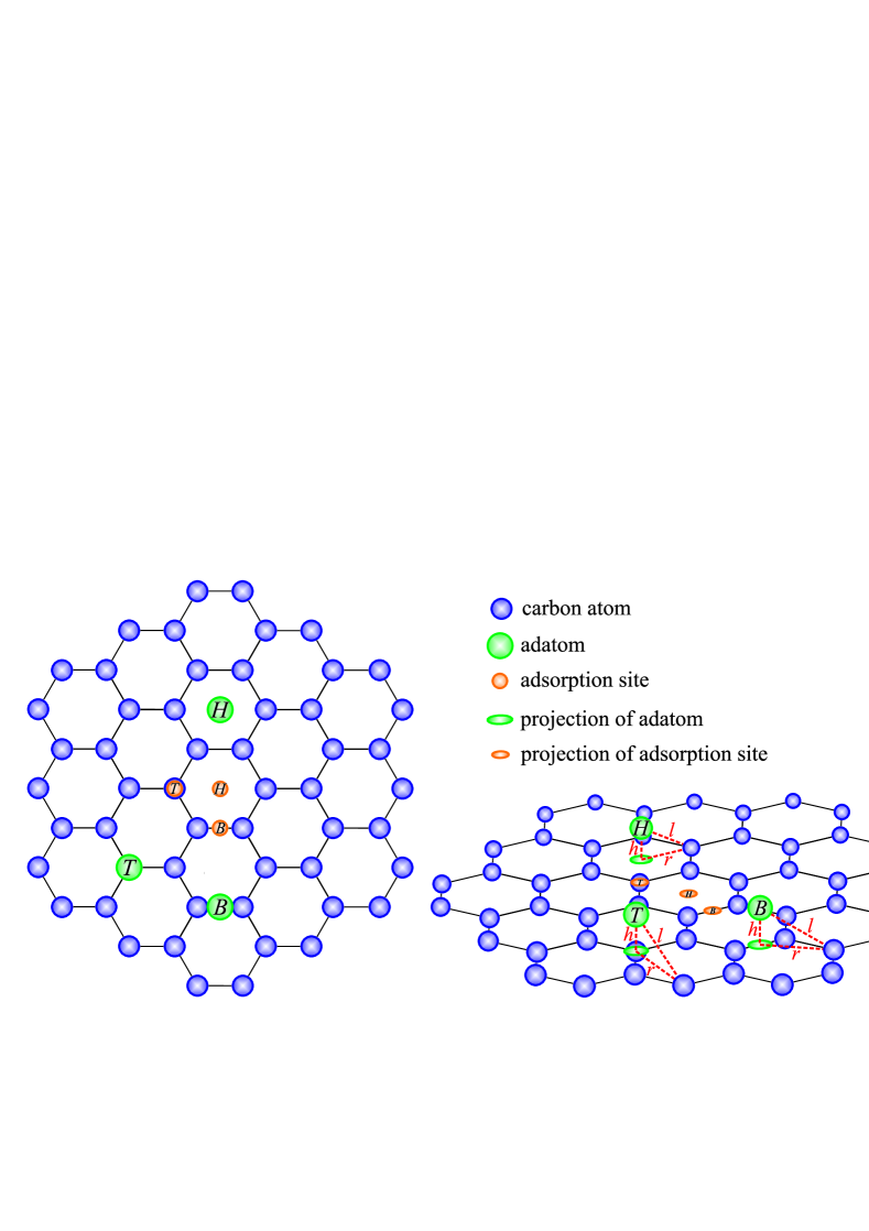
Figure 1: (Color online) Typical configurations of adatom–graphene system: top (left) and perspective (right) views of graphene lattice with hollow center (H), bridge center (B), and (a)top (T) adsorption sites.

Because of the hexagonal symmetry of the graphene lattice, possible adsorption sites for a single atom can be reduced into three types with high-symmetry positions: so-called hollow center (H-type), bridge center (B-type), and (a)top (T-type) adsorption sites as illustrated in Fig. 1. The most favorable (stable) adsorption site is determined by placing the adatom onto these three adsorption sites, and each time by optimizing structures to obtain minimum energy and atomic forces; as a result, the highest binding (adsorption) energy of adatom corresponds to its the most favorable site. Analysis of the density-functional-theory-based studies, Lugo-Solis2007 ; Uchoa2008 ; Chan2008 ; Mao2008 ; Sevincli2008 ; Zanella2008 ; Ishii2008 ; Wehling2009 ; Khomyakov2009 ; Martinez2009 ; Wang2009 ; Johll2009 ; Wu2009 ; Krasheninnikov2009 ; Malola2009 ; Suarez-Martinez2009 ; Santos2010 ; Cao2010 ; Valencia2010 ; Liu2010 ; Liu2011 ; Liu2012 ; Klintenberg2010 ; Jin2010 ; Zolyomi2010 ; Qiao2010 ; Hupalo2011 ; Ataca2011 ; Nakada2011 ; Sachs2011 ; Hardcastle2013 ; Naji2014 covering almost all the periodic table, yields: (i) for metals, the most stable adsorption sites are the H-sites, followed by the B-sites, and then the T-sites, although the energy differences between the H and B or T sites are very small for the alkali and group-III metals, particularly for potassium (see Table 1), which we regard as an example of adsorbate in the present study; (ii) for both metals and nonmetals, adsorption heights for more favorable sites are lower as compared with heights of the lesser favorable adsorption sites.

Data of Table 1 for K adsorption on graphene read that values of adsorption energy reported in the literature disagree by as much as almost 100%, while adsorption heights differ by up to 5%.Note1 Similar inconsistencies of the literature data occur also for other periodic-table elements. For example, Cu and Sn prefer T-site bonding (at the heights of 2.12 Å and 2.82 Å, respectively) according to Refs. Wu2009, and Chan2008, , while B-site bonding (2.03 Å and 2.42 Å) in accordance with Refs. Cao2010, and Nakada2011, . On the one hand, such discrepancies in determination of the energy stability of adsorption sites has resulted in a controversy and questions concerning the accuracy of theoretical models (calculations) used in those studies. On the other hand, this motivates us to study how the positioning of adatoms on each of H, B, and T site types affects the transport properties of graphene in comparison with the cases of their location on two other types of the sites.

Table 1: Literature data on calculated adsorption energies and heights for K adatoms occupying hollow (H), bridge (B), and top (T) adsorption sites in graphene.

Calculated parameter	Adsorption site
	H-type	B-type	T-type
Adsorption energy [eV]	0.785a	0.726a	0.720a
	0.802b	0.739b	0.733b
	1.461c	1.403c	1.405c
	0.810d
Adsorption height [Å]	2.62a
	2.60b	2.67b	2.67b
	2.52c	2.59c	2.55c
	2.58d

^a-dReferences Liu2011, ; Chan2008, ; Qiao2010, ; Nakada2011, (respectively).

Distributions of adatoms over the H, B, or T graphene-lattice adsorption sites are not always random, as it is usually in three-dimensional metals and alloys, where adatoms are introduced by alloying, which is generically a random process.CastroNeto2009 Diluted atoms may have a tendency towards the spatial correlationYanFuhrer2011 or even ordering.Cheianov2010 ; Cheianov2009PRB ; Cheianov2009SSC ; Howard2011 ; Song2012 ; Lin2015 Moreover, since graphene is an open surface, (ad)atoms can be positioned onto it with the use of scanning tunnelingEigler1990 or transmission electronMeyer2008 microscopes allowing to design (ad)atomic configurations as well as ordered (super)structures with atomic precision. Recently, several ordered configurations of hydrogen adatoms on graphene have been already directly observed by scanning tunneling microscopy in Ref. Lin2015, .

Though many properties of atom adsorption onto graphene have been extensively studied in many works, there is still no one paper on how such a variety of the spatial arrangements of adatoms (viz., their random, correlated, and ordered distributions in the H, B, and T types of bonding with varying adsorption heights) influences (if any) on electron transport in graphene. Such a problem formulation arises in context of the possibility to consider (ad)atomic spatial configurations as an additional tool for modification and controlling graphene’s transport properties.

Another part of our paper deals with attempt to detect adatom-mediated correlation between electron transport and electrochemical properties of graphene. Understanding of its electrochemical properties, especially the electron transfer kinetics of a redox reaction between graphene surface (electrode) and redox couple in electrolyte, is essentialVelicky2014 for its potential in energy conversion and storage to be realized,Zhao2009 ; Bonacorso2015 as well as opens up interesting opportunities for using graphene as an electrode material for field effect transistorsLi2009 ; Yan2011 and electrochemical senors.Ratinac2010 ; Lia2012 To examine the heterogeneous electron transfer kinetics at highly oriented pyrolytic graphite (HOPG) and glassy carbon (GC) electrode, several electroactive species were used.McCreery2008 Results show that electron transfer is slower at the basal plane of HOPG than at the edge plane. The kinetics of the electron transfer is enhanced after electrode pretreatment. However, in epitaxial graphene, only a part of the surface is electroactive, even after electrochemical pretreatment.Szroeder2014 Experimental results confirmed the belief that point and edge defects as well as oxygenated functional groups can mediate electron transfer.Cline1994 Contrary to the traditional view, high-resolution electrochemical imaging experiments have revealed that electron transfer occurs at both the basal planes of graphite as at the edge sites.Lai2012 To examine these discrepancies, we calculate the electron transfer kinetics at graphene with randomly-, correlatively-, and orderly-adsorbed atoms described by scattering potential manifesting both short- and long-range features, and also use strongly short-range scattering potential. Results show that electron transfer still occurs for adsorbed graphene.

The rest of the paper is organized as follows. Section II consists of two subsections containing models for electron transport and transfer. In the first subsection, we formulate the Kubo–Greenwood-formalism-based numerical model for electron transport in graphene, which is appropriate for realistic graphene sheets with millions of atoms. The size of our computational domain is up to 10 millions of atoms that corresponds to $\approx 500\times 500$ nm². The second subsection encloses the basic model we use to calculate the rate constant of electron transfer between solid (graphene) electrode and redox couple in electrolyte using the Gerischer–Marcus approach. Section III presents and discusses the obtained results. Finally, the conclusions of our work are given in Sec. IV.

II Models

II.1 Electron transport

To investigate the charge transport in adatom–graphene system, an exact numerical technique within the Kubo–Greenwood formalism, Madelung1996 ; Roche1997 ; Roche2012 ; Markussen2006 ; Triozon2002 ; Triozon2004 ; Lherbier2008_1 ; Lherbier2008_2 ; Lherbier2011 ; Leconte2011 ; Lherbier2012 ; Trambly2011 ; Ishii2010 ; Tuan2013 ; Radchenko_PRB2012 ; Radchenko_PRB2013 ; Radchenko_SSC2014 ; Radchenko_PLA2014 ; Torres2014 ; Radchenko_NOVA2014 which captures all (ballistic, diffusive, and localization) transport regimes, is employed. Within the framework of this approach, the energy ($E$) and time ($t$) dependent diffusivity $D(E,t)$Note2 is governed by the wave-packet propagation: Roche1997 ; Roche2012 ; Markussen2006 ; Triozon2002 ; Triozon2004 ; Lherbier2008_1 ; Lherbier2008_2 ; Lherbier2011 ; Leconte2011 ; Lherbier2012 ; Trambly2011 ; Ishii2010 ; Tuan2013 ; Radchenko_PRB2012 ; Radchenko_PRB2013 ; Radchenko_SSC2014 ; Radchenko_PLA2014 ; Torres2014 ; Radchenko_NOVA2014 $D(E,t)=\bigl{\langle}\Delta\hat{X}^{2}(E,t)\bigr{\rangle}/t$,Note3 where the mean quadratic spreading of the wave packet along the direction $x$ reads as Roche1997 ; Roche2012 ; Markussen2006 ; Triozon2002 ; Triozon2004 ; Lherbier2008_1 ; Lherbier2008_2 ; Lherbier2011 ; Leconte2011 ; Lherbier2012 ; Trambly2011 ; Ishii2010 ; Tuan2013 ; Radchenko_PRB2012 ; Radchenko_PRB2013 ; Radchenko_SSC2014 ; Radchenko_PLA2014 ; Torres2014 ; Radchenko_NOVA2014

$$\bigl{\langle}\Delta\hat{X}^{2}(E,t)\bigr{\rangle}=\frac{\text{Tr}[\hat{(X}(t)-\hat{X}(0))^{2}\delta(E-\hat{H})]}{\text{Tr}[\delta(E-\hat{H})]}$$ (1)

with $\hat{X}(t)=\hat{U}^{\dagger}(t)\hat{X}\hat{U}(t)$—the position operator in the Heisenberg representation, $\hat{U}(t)=e^{-i\hat{H}t/\hbar}$—the time-evolution operator, and a standard $p$-orbital nearest-neighbor tight-binding Hamiltonian $\hat{H}$ is PeresReview2010 ; DasSarmaReview2011

$$\hat{H}=-u{\textstyle\sum_{i,i^{\prime}}}c_{i}^{\dagger}c_{i^{\prime}}+{\textstyle\sum_{i}}V_{i}c_{i}^{\dagger}c_{i},$$ (2)

where $c_{i}^{\dagger}$ ($c_{i}$) is a standard creation (annihilation) operator acting on a quasiparticle at the site $i$. The summation over $i$ runs the entire honeycomb lattice, while $i^{\prime}$ is restricted to the sites next to $i$; $u=2.7$ eV is the hopping integral for the neighboring C atoms occupying $i$ and $i^{\prime}$ sites at a distance $a=0.142$ nm between them; and $V_{i}$ is the on-site potential defining scattering strength on a given graphene-lattice site $i$ due to the presence of impurity adatoms. The impurity scattering potential plays a crucial role in the transport model we use at hand.

For adatoms located on H-type sites (see Fig. 1), the impurity scattering potential in the Hamiltonian matrix is introduced as on-site energies $V_{i}$ varying with distance $r$ to the center of a hexagon on which the adatom projects according to the potential profile $V=V(r)<0$ in Fig. 2(a) adapted from the self-consistent ab initio calculationsAdessi2006 for K adatoms on the height $h\cong 2.4$ Å over the graphene surface. As the fittingFitting shows, this potential is far from the Coulomb- or Gaussian-like shapes commonly used in the literature for charged impurities in graphene, while two-exponential fitting exactly reproduces the potential. Such a scattering potential presents both short- and long-range features,Lherbier2008_2 although its short-range characteristics become rather stronger for adatoms that are nonrandom (correlated and ordered) in their spatial positions. Transforming scattering potential $V=V(r)$ into its dependence on distance from the lattice site directly to adatom, $V=V(l)$, where $l=\sqrt{r^{2}+h^{2}}$ as demonstrably from Fig. 1, one can obtain its dependence on both $r$ and $h$, $V=V(r,h)$, which is presented in Fig. 2(b). As follows from Fig. 2(b), if $r=a$ and $h=2.4$ Å $=1.69a$, $V=-0.37u$, which agrees with Fig. 2(a).

For adatoms positioned on B- and T-type sites (Fig. 1), we use the same scattering potential $V=V(r)$ as in Fig. 2(a) with difference that $r$ denotes distance from the lattice site to the middle of a C–C bond and to a C atom, respectively. Strictly speaking, $V=V(r)$ for adatoms on H-, B-, and T-type sites (Fig. 1) should be different, however just approach of the same scattering potential for these three types of adatom locations allows us to reveal manifestation of configurational effects in the transport properties of graphene we are interested in the present study.

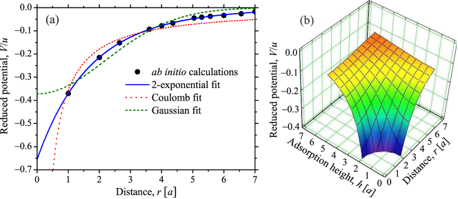
Figure 2: (Color online) Scattering potential for potassium adatoms with (a) fixed adsorption height $h=2.4$ Å and (b) varying $h$. Here, ab initio calculations ($\bullet$) Adessi2006 are fittedFitting by different functions, viz. Gaussian ($V=Ue^{-\mathbf{\mathrm{\mathit{r}}}^{2}/2\xi^{2}}$ with fitting parameters $U=-0.37u$ and $\xi=2.21a$ defining a potential height and an effective potential radius, respectively), Coulomb ($V=Q/r$ with $Q=-0.36ua$), and two-exponential ($V=U_{1}e^{-r/\xi_{1}}+U_{2}e^{-r/\xi_{2}}$ with $U_{1}=-0.45u$, $\xi_{1}=1.47a$, $U_{2}=-0.20u$, $\xi_{2}=2.73a$); $r$ is a distance from the projection of adatom to the lattice site as shown in Fig. 1.

In case of correlation, adatoms are no longer considered to be randomly located. To describe their spatial correlation, we adopt a modelLi2011 ; Li2012 using the pair distribution function $p(\mathbf{R}_{i}-\mathrm{\mathbf{R}}_{j})\equiv p(r)$:

$$p(r)=\left\{\begin{array}[]{l}0,\;r<r_{0}\\ 1,\;r\geq r_{0}\end{array}\right.$$ (3)

where $r=|\mathbf{R}_{i}-\mathbf{R}_{j}|$ is a distance between the two adatoms, and a correlation length $r_{0}$ defines minimal distance that can separate any two of them. Note that for the randomly distributed adatoms, $r_{0}=0$. Although the correlation length $r_{0}$ is found to be insensitive to impurity (potassium) density,YanFuhrer2011 the maximal correlation length $r_{0_{\mathrm{max}}}$ depends on both relative adatom concentration and positions of adsorption sites as given in Table 2. In our calculations for $n_{\mathrm{K}}=3.125\%$ of correlated (potassium) adatoms, we chose $r_{0}=r_{0_{\mathrm{max}}}^{H,B}=7a$ for hollow and bridge sites, and $r_{0_{\mathrm{max}}}^{T}=5a$ for top sites.

In case of adatom ordering, we consider superlattice structures in Fig. 3, where the relative content of ordered (potassium) adatoms is the same as for random and correlation cases, $n_{\mathrm{K}}=1/32=3.125\%$. This structures form interstitial [Fig. 3(left) and Fig. 3(center)] or substitutional [Fig. 3(right)] superstructures, where distribution of adatoms over the honeycomb-lattice interstices or sites, respectively, can be described by the single-site occupation-probability functions derived via the static concentration wave method. Khachaturyan2008 ; Radchenko-SSP2009 ; Radchenko-SSS2009 ; Radchenko-PhysE2010 ; Radchenko-SSP2008 In the computer implementation, $n_{\mathrm{K}}=3.125\%$ of potassium adatoms occupy sites within the same sublattice and can be described via a single-site function:

$$P(\mathbf{R})=\left\{\begin{array}[]{l}1,\;n_{1}+n_{2}=4\mathbb{Z}\\ 0,\;\mathrm{otherwise}\end{array}\right.$$ (4)

where $n_{1}$, $n_{2}$, and $\mathbb{Z}$ belong to the set of integers, $n_{1}$ and $n_{2}$ denote coordinates of sites in an oblique coordinate system formed by the basis translation vectors $\mathbf{a}_{1}$ and $\mathbf{a}_{2}$ shown in Fig. 3, and $\mathbf{R}$ denotes origin position of the unit cell where the considered interstice [Fig. 3(left) and Fig. 3(center)] or site [Fig. 3(right)] resides.

Table 2: Relation between the relative concentration of impurity adatoms ($n_{i}$) occupying H-, B-, or T-type sites (see Fig. 1) and the largest correlation distance ($r_{0_{\max}}$) expressed in units of the lattice parameter $a=0.142$ nm.

Site	$n_{i}$	0.5%	1%	2%	3%	4%	5%
H, B	$r_{0_{\max}}^{H,B}$ [$a$]	$18$	$13$	$9$	$7$	$6$	$5$
T	$r_{0_{\max}}^{T}$ [$a$]	$13$	$9$	$6$	$5$	$4$	$3$

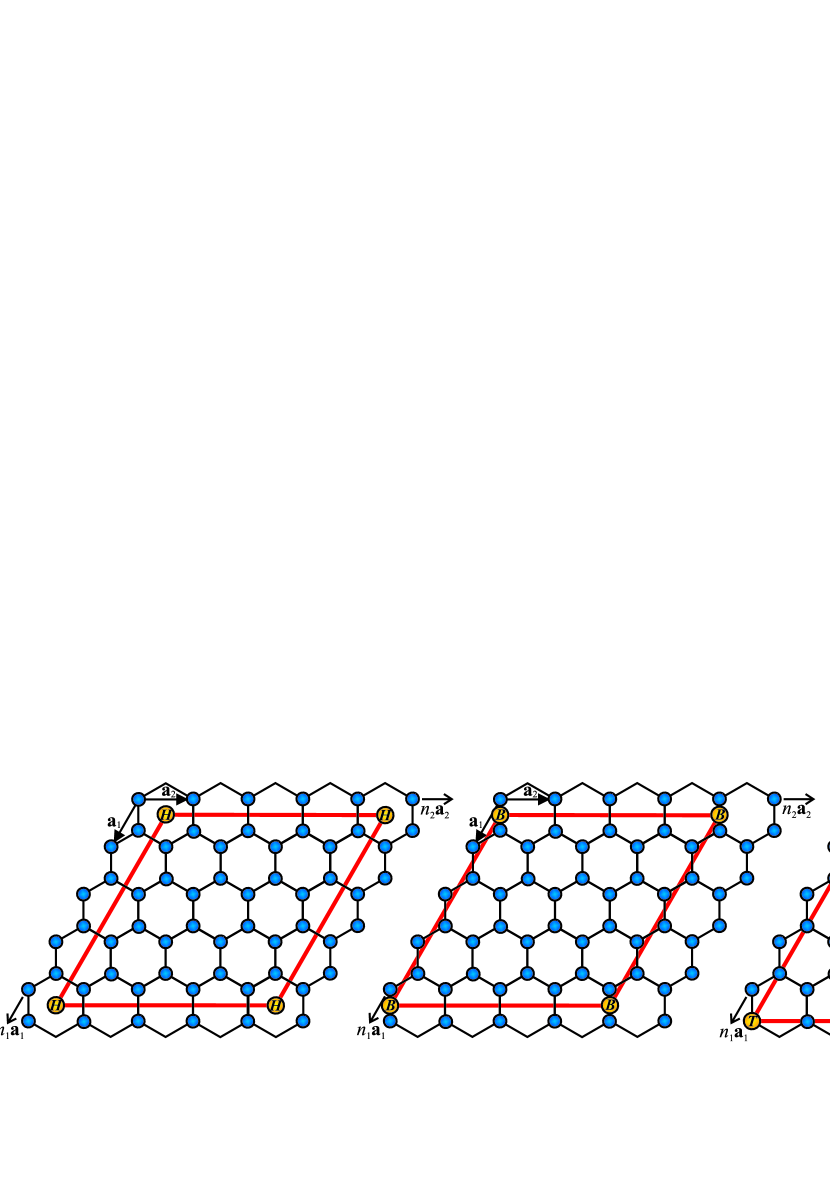
Figure 3: (Color online) Top view of graphene lattice with ordered adatoms resided on hollow (left), bridge (centre), and top (right) sites.

The dc conductivity $\sigma$ can be extracted from the diffusivity $D(E,t)$, when it saturates reaching the maximum value, $\lim_{t\rightarrow\infty}D(E,t)=D_{\max}(E)$, and the diffusive transport regime occurs. Then the semiclassical conductivity at a zero temperature is defined as Leconte2011 ; Lherbier2012

$$\sigma=e^{2}\tilde{\rho}(E)D_{\max}(E),$$ (5)

where $-e<0$ denotes the electron charge and $\tilde{\rho}(E)=\rho/\Omega=\textrm{Tr}[\delta(E-\hat{H})]/\Omega$ is the density of sates (DOS) per unit area $\Omega$ (and per spin). The DOS is also used to calculate the electron density as $n_{e}(E)=\int_{-\infty}^{E}\tilde{\rho}(E)dE-n_{\text{ions}},$ where $n_{\text{ions}}=3.9\cdot 10^{15}$ cm^-2 is the density of the positive ions in the graphene lattice compensating the negative charge of the $p$-electrons (at the neutrality (Dirac) point of pristine graphene, $n_{e}(E)=0$). Combining the calculated $n_{e}(E)$ with $\sigma(E)$, we compute the density dependence of the conductivity $\sigma=\sigma(n_{e})$.

Note that we do not go into details of numerical calculations of DOS, $D(E,t)$, and $\sigma$ since details of the computational methods, we utilize here (Chebyshev method for solution of the time-dependent Schrödinger equation, calculation of the first diagonal element of the Green’s function using continued fraction technique and tridiagonalization procedure of the Hamiltonian matrix, averaging over the realizations of impurity adatoms, sizes of initial wave packet and computational domain, boundary conditions, etc.) are given by Radchenko et al. Radchenko_PRB2012

II.2 Electron transfer

To calculate the heterogeneous rate constant of electron transfer from the reduced form of redox couple to graphene electrode, we used Gerischer–Marcus model.Gerischer1960_p223 ; Gerischer1960_p325 ; Gerischer1961 ; Gerischer1970 ; Memming2001 ; Szroeder2011 ; Szroeder2013 In this model it is assumed that electron transfer between solid electrode and redox couple in electrolyte is much faster than reorientation of the solvent molecules (diabatic representation). As a result, the rate constant of the electrode reaction depends only on the electron DOS in the solid and the distribution energy levels of the reduced (oxidized) form, $W_{\mathrm{Red\,(Ox)}}$ in the solution. If the vacuum energy as a reference energy level is chosen, the electrochemical potential of electrons occupying energy levels of ions, $\bar{\mu}_{\mathrm{e,redox}}$, is equivalent to the Fermi level of the redox couple in the solution, $E_{\mathrm{\mathit{F},redox}}$.Gerischer1983 As oxidized and reduced form interact with surrounding polar solvent in a different way, energy levels of oxidized and reduced form are shifted each other by $2\lambda$, where $\lambda$ is the reorganization energy.

In our calculations, we used the Gaussian distribution of the electronic states of the reduced form given by Memming2001

$$P(E)=\frac{1}{\sqrt{4k_{B}T\lambda}}\exp\!\left[-\frac{\left(E-E_{\mathrm{\mathit{F},redox}}-\lambda\right)^{2}}{4k_{B}T\lambda}\right],$$ (6)

where $k_{B}$ is the Boltzmann constant, $T$ is the absolute temperature. The Fe(CN)${}_{3}^{3-/4-}$ redox couple has been chosen as a benchmark system. For ferri-/ferrocyanide redox couple, the $\lambda$ value ranges between $0.5$ eV and $1.0$ eV.Bard1980 In our calculations we have used intermediate value of $0.71\,\mbox{eV}$.Szroeder2011

Dependence of the cathodic reaction rate on the electrode potential $k_{c}(V)$ is given by the integral Memming2001 ; Szroeder2011

$$k_{c}\propto\int\left[1-f(E,V)\right]\,\mbox{DOS}(E,V)\,P(E)\,dE.$$ (7)

Here, $\mbox{DOS}(E,V)=\mbox{DOS}(E-eV)$, and $f(E,V)=f(E-eV)$, where $f(E)$ is the Fermi–Dirac distribution. To determine the position of electron bands of graphene electrode in relation to the Gaussian distribution of energy levels of the reduced form, vacuum energy has been chosen as a reference. The value of $E_{F}$ in relation to the vacuum energy is equal to the work function, which has been determined experimentally for mono- and bilayer graphene using Kelvin probe force microscopy giving the $E_{F}$[vs. vacuum] $=-4.6$ eV.Yu2009

For the Fe(CN)${}_{3}^{3-/4-}$ redox couple, we used the $E_{F\mathrm{,redox}}$[vs. vacuum] value determined from the half wave potential obtained by cyclic voltammograms. Measurements carried out on epitaxial graphene and HOPG give value ranging from $V_{1/2}=-0.025$ V vs. Ag/AgCl to $V_{1/2}=0.268$ V vs. Ag/AgCl. Szroeder2014 According to Ref. Trasatti1974, , zero potential of the Ag/AgCl reference electrode is shifted in relation to the vacuum potential by $-5.04\,\mbox{V}$. Assuming the half wave potential value to be $0.20\,\mbox{V}$, we found the value of $E_{F\mathrm{,redox}}$[vs. vacuum] $=-4.84$ eV. Thus, we have assumed in our model that the Fermi level of the Fe(CN)${}_{3}^{3-/4-}$ redox couple is shifted in relation to the Fermi level of the graphene by $-1.27$ eV.

III Results and Discussion

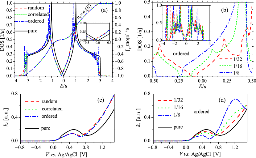
Figure 4: (Color online) (a), (b) Density of states (DOS) for (a) potential in Fig. 2(a) and for (b) short-range Gaussian potential $V=Ue^{-\mathbf{\mathrm{\mathit{r}}}^{2}/2\xi^{2}}$ (with potential height $U=-2u$ and effective potential radius $\xi=0.5a$), where (a) $3.125\%$ of random, correlated, or ordered adatoms occupy hollow sites, while (b) $3.125\%$ (stoichiometry $1/32$), $6.25\%$ ($1/16$), and $12.5\%$ ($1/8$) of ordered adatoms reside on top sites. (c), (d) Rate constant ($k_{c}$) of the cathodic reaction of oxidation of Fe(CN)${}_{3}^{4-}$ at mono-layer graphene electrode for respective (a), (b) DOS. Insets in (a) and (b) show the same as in the main panels, but with another scales. As a reference, DOS (a) and rate constant (c), (d) for pure graphene electrode are shown.

As it was mentioned in Secs. I and II, we consider potassium as an example of adsorbate in the present study. The most energy favorable adsorption sites for K dopants in graphene are H-type sites as listed in Table 1. Therefore results obtained at potential in Fig. 2(a) and H-type sites are appropriate for K adsorbed graphene first of all. Results obtained for B- and T-type sites can be associated with K adsorbate in a model assumption for revealing manifestation of configurational effects in electron transport.

Figure 4(a) shows the DOS and the electron density $n_{e}=n_{e}(E)$ for graphene with $n_{\mathrm{K}}=3.125\%$ of random, correlated, and ordered potassium adatoms, which are described by the scattering potential in Fig. 2(a) and are distributed over the H-type adsorption sites. DOS-curves for B- and T-type are similar to those shown in Fig. 4(a) with difference that Fermi level in case of T sites is shifted more far with respect to $E=0$ to the (left) side of negative $E<0$—energies of holes in our denotations. The Dirac (neutrality) point shifts towards negative energies (gate voltage) due to electron (n-type) doping dictated by the asymmetry (negativity) of the scattering potential. The calculated DOS-curves in Fig. 4(a) for random, correlated, and ordered K adatoms are similar with two differences take place in the case of ordering: (i) peaks (fluctuations), which appear close to $E/u\approx-3$ at correlation, begin to manifest themselves in all energy interval (weakly away from the regions of the van Hove singularities and $|E/u|\approx 3$, but stronger close to them); (ii) at a Fermi energy level, the DOS drops to zero (but even small band gap does not open). Appearing of the peaks (fluctuations) in DOS is due to the periodicity of the scattering-potential distribution describing ordered positions of adatoms on the sites of interstitial [Figs. 3(left) and 3(center)] or substitutional [Fig. 3(right)] graphene-based superstructure. Additional calculationsRadchenko_NOVA2014 [see also inset in Fig. 4(b)] show that the peaks become stronger and even transform into discrete energy levels with broadening as impurity concentration and/or periodic potential increase.

Positioning of ordered adatoms on the T-type sites [Fig. 3(right)] makes possible band gap opening, which is clearly seen in Fig. 4(b) for a strongly short-range, e.g., Gaussian potential with very small effective potential radius $\xi<a$. The band gap is induced by the periodic potential leading to the ordered distribution of adatoms directly above the C atoms belonging to the same sublattice, thus breaking of symmetry of two graphene sublattices. Note that adatoms on T sites act as substitutional point defects—impurities or vacancies—which can also induce the band gap opening if they are distributed orderly Cheianov2010 ; Park2008 ; Martinazzo2010 ; Casolo2011 ; Radchenko_PLA2014 or belong to the same sublattice even being randomly located. Lherbier2013 ; Pereira2008 However, we did not observe the band gap appearing if ordered adatoms reside on H and B adsorption sites (thereby act as interstitial dopants) as it is reported by Cheianov et al. for adatoms occupying H Cheianov2009SSC and B Cheianov2009PRB sites. We attribute the lack of the band gap opening (when ordered adatoms occupy H and B sites) to the absence of the breaking of global lattice symmetry in these cases.

Obtained densities of electronic states enter into Eq. (7) and thereby enable us to calculate the electrode-potential-dependent rate constants at various adatomic configurations as well as concentrations. Figure 4(c) demonstrates the rate constant of the reaction of oxidation of ferrocyanide ions, $k_{c}$, at graphene electrode with potassium impurity as a function of electrode potential. At a potential of about $-0.1$ V vs. Ag/AgCl, increase of the cathodic reaction rate is observed. Contrary to metallic electrodes, the increase of the $k_{c}$ is not monotonic. In the range of calculated potentials, the plot of $k_{c}$ vs. $V$ has a hump. The local minimum appears within the electrochemical window of water, i.e. within the range $0.6\mathrm{-}0.8$ V vs. Ag/AgCl. The monotonic increase is observed at the positive electrode potentials beyond the water window ($V>0.8$ V vs. Ag/AgCl). Difference between the $k_{c}$ vs. $V$ plots calculated for the pure graphene and graphene with K adatoms is seen clearly. However, as well as the shape of DOS-curves close to the Dirac point [Fig. 4(a)], the shape of $k_{c}$-plots of impure graphene [Fig. 4(c)] is only negligibly affected by the impurity configuration. Generally, K-impurity slow down the reaction kinetics in the electrode potentials in the range of water window. At the pure graphene electrode, the maximum of the hump is located at potential of $0.503\,\mbox{V}$ vs. Ag/AgCl ($k_{c}=0.194$ a.u.), whereas at graphene with K adatoms in the concentration of $3.125\%$ the maximum is observed at lower potential of $0.453\,\mbox{V}$ vs. Ag/AgCl ($k_{c}=0.123$ a.u.). The same applies to the position of the local minimum, which is downshifted in graphene with K adatoms by $0.17\,\mbox{V}$.

Contrary to the impurity configuration, the concentration of adatoms influences strongly the $k_{c}$ [Fig. 4(d)] similarly to the influence on the DOS [Fig. 4(b)]. With increasing adatomic concentration, the position of the local maximum shift towards lower potentials from the value of $0.503$ V vs. Ag/AgCl ($k_{c}=0.123$ a.u.) for pure graphene to $0.393$ V vs. Ag/AgCl ($k_{c}=0.091$ a.u.). Also the local minimum shifts down form the potential value of $0.843$ V vs. Ag/AgCl to $0.393$ V vs. Ag/AgCl to $0.573$ V vs. Ag/AgCl for pure graphene and graphene with adatomic concentration of $12.5\%$, respectively. In a part of the $k_{c}$ plot in the range of higher potentials ($V>0.8$ V vs. Ag/AgCl) an additional hump is apparent at $12.5\%$ of adatoms.

Assuming $0.2$ V vs. Ag/AgCl as a standard electrode potential (when the rates of both cathodic and anodic reactions are equal), in Table 3 we compare values of the standard rate constant, $k_{s}$, for electron transfer between the Fe(CN)${}_{3}^{3-/4-}$ redox couple and impure graphene at weakly long-range scattering potential in Fig. 2(a) and strongly short-range Gaussian potential $V=Ue^{-\mathbf{\mathrm{\mathit{r}}}^{2}/2\xi^{2}}$ with potential height $U=-2u$ and effective potential radius $\xi=0.5a$. While the adatomic configurations do not affect significantly the shape of the $k_{c}$ plot, apparent differences in the $k_{s}$ at different ranges of the scattering potential action are seen. When the long-range potential is used, the electron transfer is moderately suppressed by adatoms in random ($\approx$31%), correlated ($\approx$33%), and ordered ($\approx$32%) configurations as compared to the electron transfer of pure graphene. On the other hand, weak dependence between impurity concentration and the $k_{s}$ value is observed if the short-range potential is used; quadrupling the adatomic content causes the decrease of $k_{s}$ by only $\approx$23%. Thus, the use of the long-range potential more strongly suppresses the electron transfer kinetics. It is worth noting that the best kinetics is observed at pure electrode. Our findings are not compatible with experimental results obtained in Ref. McCreery2008, . Discrepancies are probably due to the hydrophobic properties of graphene.

Table 3: Standard rate constants, $k_{s}$, for electron transfer between graphene electrode and ferro-/ferricyanide redox couple for different ranges of the scattering-potential action, adatomic configurations and concentrations.

Type of potential	Configuration	Stoichiometry	$k_{\mathrm{\mathit{s}}}$ [a.u.]
Long-range	Random	1/32 (3.125%)	0.0595
	Correlated		0.0571
	Ordered		0.0586
Short-range	Ordered	1/32 (3.125%)	0.0791
		1/16 (6.25%)	0.0740
		1/8 (12.5%)	0.0610
	Pure	0	0.0858

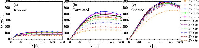
Figure 5: (Color online) Time-dependent diffusivity within the energy range $E\in[-0.5u,0.5u]$ for random (a), correlated (b), and ordered (c) potassium adatoms located on hollow sites.

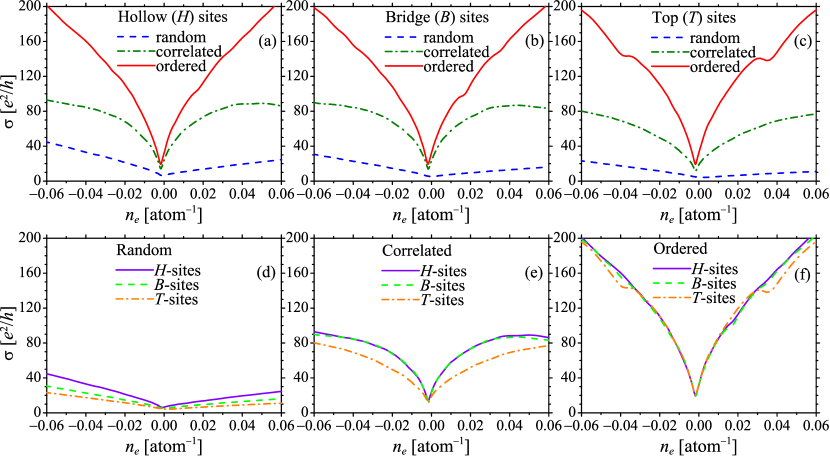
Figure 6: (Color online) Conductivity vs. the electron density for $n_{\mathrm{K}}=3.125\%$ of random, correlated, and ordered potassium adatoms occupying hollow (H), bridge (B), or top (T) adsorption sites. Curves in upper and lower figures are the same, but grouped in a different way to distinguish configuration effects induced by correlation or ordering from those caused by difference in type of adsorption sites: H, B, or T.

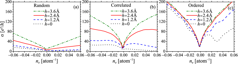
Figure 7: (Color online) Electron-density-dependent conductivity for different adsorption heights, h, of $3.125\%$ of random (a), correlated (b), and ordered (c) K adatoms resided on hollow sites.

In contrast to the case of randomly-arranged adatoms, when steady diffusive regime is reached for a relatively short time [Fig. 5(a)], in case of their correlation and especially ordering, a quasi-ballistic regime is observed during a long time as it is shown in Figs. 5(b) and (c). This (quasi-ballistic) behavior of diffusivity, $D(t)$, indicates a very low scattered electronic transport, at which maximal value of $D(t)$ is substantially higher for correlated and much more for ordered adatoms as compared with their random distribution. If the diffusive regime is not completely reached, the semiclassical conductivity, $\sigma$, cannot be in principle defined. However, we extracted $\sigma$ for the case of ordered adatoms using the highest $D(t)$ when quasi-ballistic behavior turns to a quasi-diffusive regime with an almost saturated diffusivity coefficient.

Figure 6 represents calculated conductivity ($\sigma$) as a function of electron ($n_{e}>0$) or hole ($n_{e}<0$) concentration, $\sigma=\sigma(n_{e})$, for different positions (viz. H, B, and T) and distributions (viz. random, correlated, and ordered) of adatoms in graphene. For visual convenience, we arranged the same (nine) curves in two groups: Figs. 6(a)–(c) demonstrate how correlation and ordering affect the conductivity for each of H, B, and T adsorption types, while Figs. 6(d)–(f) exhibit how these three types of sites influence on the conductivity for each of random, correlated (with maximal correlation lengths as listed in Table 2), and ordered adatomic distributions. The conductivity exhibits linear or nonlinear (viz. sublinear) electron-density dependencies. The linearity of $\sigma=\sigma(n_{e})$ takes place at randomly-distributed potassium adatoms and indicates dominance of the long-range contribution to the scattering potential, while sublinearity occurs at nonrandom (viz. correlated and ordered) positions of K adatoms and is indicative of the dominance of short-range component of the scattering potential. This is in accordance with many previous studies (see, e.g., Ref. Radchenko_PRB2012 and references therein) in which pronounced linearity and sublinearity of $\sigma=\sigma(n_{e})$ are observed for long-range scattering potential (appropriate for screened charged impurities ionically bond to graphene) and short-range potential (appropriate for neutral covalently bond adatoms), respectively. These results illustrate manifestation of contrasting scattering mechanisms for different spatial distributions of metallic adatoms.

One can see from Figs. 6(a)–(c) that conductivities for correlated ($\sigma_{\mathrm{cor}}$) and ordered ($\sigma_{\mathrm{ord}}$) adatoms are dozens of times enhanced as compared with case of randomly-distributed adatoms ($\sigma_{\mathrm{rnd}}$). These enhancements ($\sigma_{\mathrm{cor}}/\sigma_{\mathrm{rnd}}$ and $\sigma_{\mathrm{ord}}/\sigma_{\mathrm{rnd}}$) depends on electron density and type of adsorption sites. It is easy to determine from Figs. 6(a)–(c) that the ratio $\sigma_{\mathrm{cor}}/\sigma_{\mathrm{rnd}}$ ranges as 2 $\lesssim$ $\sigma_{\mathrm{cor}}^{H}(n_{e})/\sigma_{\mathrm{rnd}}^{H}(n_{e})$ $\lesssim$ 5, 2 $\lesssim$ $\sigma_{\mathrm{cor}}^{B}(n_{e})/\sigma_{\mathrm{rnd}}^{B}(n_{e})$ $\lesssim$ 6, and 3 $\lesssim$ $\sigma_{\mathrm{cor}}^{T}(n_{e})/\sigma_{\mathrm{rnd}}^{T}(n_{e})$ $\lesssim$ 7; while $\sigma_{\mathrm{ord}}/\sigma_{\mathrm{rnd}}$ ranges as 3 $\lesssim$ $\sigma_{\mathrm{ord}}^{H}(n_{e})/\sigma_{\mathrm{rnd}}^{H}(n_{e})$ $\lesssim$ 8, 3 $\lesssim$ $\sigma_{\mathrm{ord}}^{B}(n_{e})/\sigma_{\mathrm{rnd}}^{B}(n_{e})$ $\lesssim$ 9, and 4 $\lesssim$ $\sigma_{\mathrm{ord}}^{T}(n_{e})/\sigma_{\mathrm{rnd}}^{T}(n_{e})$ $\lesssim$ 15 (here, superscripts denote types of adsorption sites). As follows from Figs. 6(d)–(f), in a random adatomic state $\sigma_{\mathrm{rnd}}^{T}$ $<$ $\sigma_{\mathrm{rnd}}^{B}$ $<$ $\sigma_{\mathrm{rnd}}^{H}$, while for correlated and ordered states, $\sigma_{\mathrm{cor}}^{T}$ $<$ $\sigma_{\mathrm{cor}}^{B}$ $\approx$ $\sigma_{\mathrm{cor}}^{H}$ and $\sigma_{\mathrm{ord}}^{T}$ $\approx$ $\sigma_{\mathrm{ord}}^{B}$ $\approx$ $\sigma_{\mathrm{ord}}^{H}$, respectively. That is why the highest increase of $\sigma$ due to correlation ($\sigma_{\mathrm{cor}}/\sigma_{\mathrm{rnd}}$) or ordering ($\sigma_{\mathrm{ord}}/\sigma_{\mathrm{rnd}}$) takes place for the T-site bonding, followed by the B sites, and then the H sites. The increasing of $\sigma$ due to adatomic correlation or ordering is expected in a varying degree for any constant-sign ($V>0$ or $V<0$) scattering potential, but this is not the case when the potential is sign-changing ($V\gtrless 0$).Radchenko_PRB2012

If adatoms are randomly-positioned on the (H, B, or T) adsorption sites, the conductivity is dependent on their type: $\sigma_{\mathrm{rnd}}^{H}$ $>$ $\sigma_{\mathrm{rnd}}^{B}$ $>$ $\sigma_{\mathrm{rnd}}^{T}$, particularly $\sigma_{\mathrm{rnd}}^{H}$ $\thickapprox$ $2\sigma_{\mathrm{rnd}}^{T}$ [Fig. 6(d)]. Here, the differences in $\sigma$ are caused by different values of on-site potentials for these three types of adatomic positions although the same potential profile $V=V(r)$ [Fig. 2(a)] is used for them. The stronger (weaker) on-site potential $V_{i}$ corresponds to the smaller (larger) distance $r$ from the given graphene-lattice site $i$ to the nearest adsorption site, which is more close (distant) for the H (T) type, followed by the B type, and then the T (H) type. If adatoms are correlated, the conductivity is dependent on whether they act as interstitial (H or B sites) or substitutional (T sites) atoms: $\sigma_{\mathrm{cor}}^{H}$ $\approx$ $\sigma_{\mathrm{cor}}^{B}$ $>$ $\sigma_{\mathrm{cor}}^{T}$ [Fig. 6(e)], which can be attributed to the values of maximal correlation lengths (Table 2) defining correlation degree for H, B and T sites, $r_{0_{\max}}^{H}$ $=$ $r_{0_{\max}}^{B}$ $>$ $r_{0_{\max}}^{T}$. Finally, if adatoms form ordered superstructures (superlattices) with equal periods (Fig. 3), the conductivity is practically independent on the adsorption type (especially for not very high charge carrier densities): $\sigma_{\mathrm{ord}}^{H}$ $\approx$ $\sigma_{\mathrm{ord}}^{B}$ $\approx$ $\sigma_{\mathrm{ord}}^{T}$ [Fig. 6(f)].

In our model, increase (or decrease) of adatomic elevation over the graphene surface results to more weak (or strong) scattering-potential amplitude, i.e. physically it means more weak (or strong) regime of electron scattering on charged impurity adatoms. Although the values of adsorption height, $h$, reported in the literature for potassium do not disagree as much as for the adsorption energy (see Table 1), for the model and calculation completeness, we range $h$ in a wide interval (up to $h=3.6$ Å) including an exotic case of $h=0$, when impurity atoms act as strictly interstitial ones. Calculated curves representing the charge-carrier-density-dependent conductivity for (random, correlated, and ordered) adatoms resided on (the most favorable for potassium) hollow sites and elevated on different $h$ are shown in Fig. 7. (Here, we do not consider the cases of less favorable for potassium bridge and top sites since it leads to qualitatively the same results.) As follows from Figs. 7(a) and (b), at least for hole densities ($-n_{e}>0$), two (three) time increased or decreased $h$ for randomly- or correlatively-distributed K-adatoms results to approximately two (three) time enhanced or reduced $\sigma$, respectively. Thus the conductivity approximately linearly scales with adsorption height of random or correlated adatoms, $\sigma(h)\propto h$. However, for ordered potassium adatoms, the $\sigma$ remains practically unchanged with varying of $h$ in the realistic range of adsorption heights (see Table 1) and even in all range at issue ($0\leqslant h\leqslant 3.6$ Å) for hole densities [Fig. 7(c)]. We attribute this to the dominance of short-range scatterers in case of their ordered state as it was mentioned above. Indeed, the Gaussian fitting for the scattering potential in Fig. 2(a) yields the effective potential radius $\xi=2.21a$, which is commensurable with quantities of adsorption heights $h$ at issue (and even less than $h=3.6$ Å).

In conclusion of this section, note that our numerical calculations of conductivity in Figs. 6 and 7 agree with experimentally observed features of $\sigma=\sigma(n_{e})$ in potassium-doped graphene:Chen2008 ; YanFuhrer2011 (i) asymmetry in the conductivity for electrons versus holes (which, however, can be weakened and even totally suppressed due to the spatial correlation or especially ordering of adatoms as well as increasing of their adsorption height), (ii) shifting of minimum conductivity at a charge neutrality point to more negative gate voltage, (iii) linearity or sublinearity of conductivity at lower or higher gate voltage, respectively, and (iv) increase in conductivity due to correlation in the positions of adatoms that was also sustained theoreticallyLi2011 within the standard semiclassical Boltzmann approach in the Born approximation. A significant sublinear behavior of electron-density-dependent conductivity and its saturation for very high densities at the spatial correlations among the charged impurity locations in contrast to the strictly linear-in-density graphene conductivity for uncorrelated random charged impurity scattering [Figs. 6(a)–(e) and 7(a)–(b)] is also in agreement with theoretical findings in Refs. Li2011, and Li2012, .

IV Conclusions

By employing numerical calculations, we systematically studied the effects of different (random, correlated, and ordered) spatial configurations of potassium adatoms onto high-symmetry [hollow- (H), bridge- (T), and top-type (T)] adsorption sites with various elevations over the graphene sheet on its electron transport and electrochemical properties to ascertain correlation between them. We conclude as follows.

(i) The charge carrier density dependence of the conductivity is indicative of dominance of long-range scattering centers for their random spatial distribution, while short-range scatterers dominate for their correlated and ordered states. This demonstrates manifestation of contrasting scattering mechanisms for different spatial distributions of metallic adatoms.

(ii) A band gap may be opened only if ordered adatoms act as substitutional atoms (i.e. reside on T-type sites) due to the breaking of graphene lattice point symmetry, while there is no band gap opening for adatoms acting as interstitial atoms (i.e. occupying H- or B-type sites).

(iii) If adatoms are randomly-positioned on the H, B- or T sites, the conductivity is dependent on their type: $\sigma_{\mathrm{rnd}}^{H}$ $>$ $\sigma_{\mathrm{rnd}}^{B}$ $>$ $\sigma_{\mathrm{rnd}}^{T}$. For spatially-correlated adatoms, the conductivity is dependent on whether they act as interstitial or substitutional atoms: $\sigma_{\mathrm{cor}}^{H}$ $\approx$ $\sigma_{\mathrm{cor}}^{B}$ $>$ $\sigma_{\mathrm{cor}}^{T}$. If adatoms form ordered superstructures (superlattices) with equal periods, the conductivity is practically independent on the adsorption type (especially for low electron densities): $\sigma_{\mathrm{ord}}^{H}$ $\approx$ $\sigma_{\mathrm{ord}}^{B}$ $\approx$ $\sigma_{\mathrm{ord}}^{T}$.

(iv) Depending on electron density and type of adsorption sites, the conductivity for correlated and ordered K adatoms is found to be enhanced in dozens of times as compared to the cases of their random positions. The correlation and ordering effects manifest stronger for adatoms acting as substitutional atoms and weaker for those acting as interstitial atoms.

(v) The electron–hole asymmetry in the conductivity for randomly-positioned adatoms weakens and even may be totally suppressed for correlated and especially ordered ones as well as for increased of their adsorption height.

(vi) The conductivity dependence with adsorption height of random or correlated adatoms scales approximately as $\sigma(h)\propto h$. However, for ordered adatoms, $\sigma$ remains practically unchanged with varying of $h$ within its realistic range.

(vii) Only slight suppress of electron transfer kinetics in electrolyte at K-doped graphene electrode is revealed. Strong correlation between the band gap in graphene and the shape of the electrode-potential dependence of electrochemical rate constant is seen, when the strongly short-range scattering potential during the electron transport in graphene is used. At the same time, the influence of this potential on the suppress of the standard electrochemical rate constant is much weaker as compared to the case of the long-range electron-scattering potential in graphene. Comparison of the electron transfer calculations to experiment shows that the hydrophobicity of graphene is a key factor, which suppresses the kinetics of heterogeneous electron transfer in electrolyte at graphene electrode.

- (1) M. I. Katsnelson, Graphene: Carbon in Two Dimensions (Cambridge University Press, New York, 2012).
- (2) Z. Jia, B. Yan, J. Niu, Q. Han, R. Zhu, D. Yu, and X. Wu, Phys. Rev. B 91, 085411 (2015).
- (3) K. M. McCreary, K. Pi, and R. K. Kawakami, Appl. Phys. Lett. 98, 192101 (2011).
- (4) Y. Gan, L. Sun, and F. Banhart, Small 4, 587 (2008).
- (5) J.-H. Chen, C. Jang, S. Adam, M. S. Fuhrer, E. D. Williams, and M. Ishigami, Nature Phys. 4, 377 (2008).
- (6) C. Uthaisar, V. Barone, and J. E. Peralta, J. Appl. Phys. 106, 113715 (2009).
- (7) Y. Kubota, N. Ozava, H. Nakanishi, and H. Kasai, J. Phys. Soc. Jpn. 79, 014601 (2010).
- (8) C. Vo-Van, Z. Kassir-Bodon, H.Yang, J. Coraux, J. Vogel, S. Pizzini, P. Bayle-Guillemaud, M. Chshiev, L. Ranno, V. Guisset, P. David, V. Salavador, and O. Fruchart, New J. Phys. 12, 103040 (2010).
- (9) J. A. Rodríguez-Manzo, O. Cretu, and F. Banhart, ACS Nano 4, 3422 (2010).
- (10) J. H. Garcia, B. Uchoa, L. Covaci, and T. G. Rappoport, Phys. Rev. B 90, 085425 (2014).
- (11) Y. Virgus, W. Purwanto, H. Krakauer, and S. Zhang, Phys. Rev. Lett. 113, 175502 (2014).
- (12) V. Sessi, S. Stepanow, A. N. Rudenko, S. Krotzky, K. Kern, F. Hiebel, P. Mallet, J.-Y. Veuillen, O. Šipr, and J. Honolka, New J. Phys. 16, 062001 (2014).
- (13) A. H. Castro Neto, V. N. Kotov, J. Nilsson, V. M. Pereira, N. M. R. Peres, and B. Uchoa, Solid State Comm. 149, 1094 (2009).
- (14) B. Uchoa, C.-Y. Lin, and A. H. Castro Neto, Phys. Rev. B 77, 035420 (2008).
- (15) H. Sevincli, M. Topsakal, E. Durgun, and S. Ciraci, Phys. Rev. B 77, 195434 (2008).
- (16) I. Zanella, S. B. Fagan, R. Mota, and A. Fazzio, J. Phys. Chem. C 112, 9163 (2008).
- (17) Y. L. Mao, J. M. Yuan, and J. X. Zhong, J. Phys.: Condens. Matter. 20, 115209 (2008).
- (18) S. Malola, H. Häkkinen, and P. Koskinen, Appl. Phys. Lett. 94, 043106 (2009).
- (19) Q. E. Wang, F. H. Wang, J. X. Shang, and Y. S. Zhou, J. Phys.: Condens. Matter. 21, 485506 (2009).
- (20) I. S.-Martinez, A. Felten, J. J. Pireaux, C. Bittencourt, and C. P. Ewels, J. Nanosci. Nanotechnol. 9, 6171 (2009).
- (21) H. Johll, H. C. Kang, and E. S. Tok, Phys. Rev. B 79, 245416 (2009).
- (22) M. Wu, E.-Z. Liu, M. Y. Ge, and J. Z. Jiang, Appl. Phys. Lett. 94, 102505 (2009).
- (23) P. A. Khomyakov, G. Giovannetti, P. C. Rusu, G. Brocks, J. van den Brink, and P. J. Kelly, Phys. Rev. B 79, 195425 (2009).
- (24) A. V. Krasheninnikov, P. O. Lehtinen, A. S. Foster, P. Pyykko, and R. M. Nieminen, Phys. Rev. Lett. 102, 126807 (2009).
- (25) K.-H. Jin, S.-M. Choi, and S.-H. Jhi, Phys. Rev. B 82, 033414 (2010).
- (26) V. Zólyomi, Á . Rusznyák, J. Kürti, and C. J. Lambert, J. Phys. Chem. C 114, 18548 (2010).
- (27) E. J. G. Santos, A. Ayuela, and D. Sánchez-Portal, New J. Phys. 12, 053012 (2010).
- (28) X. Liu, C. Z. Wang, M. Hupalo, Y. X. Yao, M. C. Tringides, W. C. Lu, and K. M. Ho, Phys. Rev. B 82, 245408 (2010).
- (29) M. Hupalo , X. Liu , C.-Z. Wang , W.-C. Lu , Y.-X. Yao , K.-M. Ho , and M. C. Tringides, Adv. Mater. 23, 2082 (2011).
- (30) A. Lugo-Solis and I. Vasiliev, Phys. Rev. B 76, 235431 (2007).
- (31) I. Suarez-Martinez, A. Felten, J. J. Pireaux, C. Bittencourt, Ch. P. Ewels, J. Nanoscience and Nanotechnol. 9, 6171 (2009).
- (32) X. Liu, C. Z. Wang, M. Hupalo, W. C. Lu, M. C. Tringides, Y. X. Yaoa, and K. M. Hoa, Phys. Chem. Chem. Phys. 14, 9157 (2012).
- (33) C. Cao, M. Wu, J. Jiang, and H.-P. Cheng, Phys. Rev. B 81, 205424 (2010).
- (34) H. Valencia, A. Gil, and G. Frapper, J. Phys. Chem. C 114, 14141 (2010).
- (35) T. P. Hardcastle, C. R. Seabourne, R. Zan, R. M. D. Brydson, U. Bangert, Q. M. Ramasse, K. S. Novoselov, and A. J. Scott, Phys. Rev. B 87, 195430 (2013).
- (36) S. Naji, A. Belhaj, H. Labrim, M. Bhihi, A. Benyoussef, and A. El Kenz, Int. J. Quantum Chemistry 114, 463 (2014).
- (37) X. Liu, C. Z. Wang, Y. X. Yao, W. C. Lu, M. Hupalo, M. C. Tringides, and K. M. Ho, Phys. Rev. B 83, 235411 (2011).
- (38) K. T. Chan, J. B. Neaton, and M. L. Cohen, Phys. Rev. B 77, 235430 (2008).
- (39) L. Qiao, C. Q. Qu, H. Z. Zhang, S. S. Yu, X. Y. Hu, X. M. Zhang, D. M. Bi, Q. Jiang, and W. T. Zheng, Diamond & Related Materials 19, 1377 (2010).
- (40) K. Nakada and A. Ishii, Solid State Comm. 151, 13 (2011); K. Nakada and A. Ishii, in Graphene Simulation, edited by J. R. Gong (InTech, 2011), Ch. 1, pp. 3–20.
- (41) A. Ishii, M. Yamamoto, H. Asano, and K. Fujiwara, J. Phys.: Conf. Ser. 100, 052087 (2008).
- (42) B. Sachs, T. O. Wehling, A. I. Lichtenstein, and M. I. Katsnelson, in Physics and Applications of Graphene—Theory, edited by Sergey Mikhailov (InTech, 2011), pp. 29–44.
- (43) T. O. Wehling, M. I. Katsnelson, and A. I. Lichtenstein, Phys. Rev. B 80, 085428 (2009).
- (44) M. Klintenberg, S. Lebegue, M. I. Katsnelson, and O. Eriksson, Phys. Rev. B 81, 085433 (2010).
- (45) C. Ataca, E. Aktürk, H. Şahin, and S. Ciraci, J. Applied Phys. 109, 013704 (2011).
- (46) M. Wu, E.-Z. Liu, and J. Z. Jianga, Appl. Phys. Lett. 93, 082504 (2008).
- (47) Y. G. Zhou, X. T. Zu, F. Gao, J. L. Nie, and H. Y. Xiao, J. Appl. Phys. 105, 014309 (2009).
- (48) H. Gao, J. Zhou, M. Lu, W. Fa, and Y. Chen, J. Appl. Phys. 107, 114311 (2010).
- (49) V. V. Ivanovskaya, A. Zobelli, D. Teillet-Billy, N. Rougeau, V. Sidis, and P. R. Briddon, Eur. Phys. J. B 76, 481 (2010).
- (50) C. Lin, Y. Feng, Y. Xiao, M. Dürr, X. Huang, X. Xu, R. Zhao, E. Wang, X.-Z. Li, and Z. Hu, Nano Lett. 15, 903 (2015).
- (51) S. Yuan, H. De Raedt and M. I. Katsnelson, Phys. Rev. B 82, 115448 (2010).
- (52) Inconsistency of the literature data have been also reported in Ref. Lugo-Solis2007, , where in Table I adsorption energies and heights for K-graphene clusters differ by as much as 350% and up to 3%, respectively, but not 400% and 12% as authorsLugo-Solis2007 pointed out.
- (53) J. Yan and M. S. Fuhrer, Phys. Rev. Lett. 107, 206601 (2011).
- (54) V. V. Cheianov, O. Syljuåsen, B. L. Altshuler, and V. I. Fal’ko, Eur. Phys. Lett. 89, 56003 (2010).
- (55) V. V. Cheianov, V. I. Fal’ko, O. Syljuasen, and B. L. Altshuler, Solid State Comm. 149, 1499 (2009).
- (56) V. V. Cheianov, O. Syljuasen, B. L. Altshuler, and V. I. Fal’ko, Phys. Rev. B 80, 233409 (2009).
- (57) C. A. Howard, M. P. M. Dean, and F. Withers, Phys. Rev. B 84, 241404(R) (2011).
- (58) C.-L. Song, B. Sun, Y.-L. Wang, Y.-P. Jiang, L. Wang, K. He, X. Chen, P. Zhang, X.-C. Ma, and Q.-K. Xue, Phys. Rev. Lett. 108, 156803 (2012).
- (59) D. M. Eigler and E. K. Schweizer, Nature 344, 524 (1990).
- (60) J. C. Meyer, C. O. Girit, M. F. Crommie, and A. Zettl, Nature 454, 319 (2008).
- (61) M. Velický, D. F. Bradley, A. J. Cooper, E. W. Hill, I. A. Kinloch, A. Mishchenko, K. S. Novoselov, H. V. Patten, P. S. Toth, A. T. Valota, S. D. Worrall, and R. A. W. Dryfe, ACS Nano, 8, 10089 (2014).
- (62) L. Zhao, L. Zhao, Y. Xu, T. Qiu, L. Zhi, and G. Shi, Electrochim. Acta 55, 491 (2009).
- (63) F. Bonaccorso, L. Colombo, G. Yu, M. Stoller, V. Tozzini, A. C. Ferrari, R S. Ruoff, and V. Pellegrini, Science 347, 1246501 (2015).
- (64) X. Li, Y. Zhu, W. Cai, M. Borysiak, B. Han, D. Chen, R. D. Piner, L. Colombo, and R. S. Ruoff, Nano Lett. 9, 4359 (2009).
- (65) Z. Yan, Z. Sun, W. Lu, J. Yao, Y. Zhu, and J. M. Tour, ACS Nano 5, 1535 (2011).
- (66) K. R. Ratinac, W. Yang, J. J. Gooding, P. Thordarson, and F. Braet, Electroanalysis 23, 803 (2010).
- (67) X.-R. Lia, J. Liua, F.-Y. Konga, X.-C. Liub, J.-J. Xua, and H.-Y. Chen, Electrochem. Comm. 20, 109 (2012).
- (68) R. L. McCreery, Chem. Rev. 108, 2646 (2008).
- (69) P. Szroeder, N. G. Tsierkezos, M. Walczyk, W. Strupiński, A. Górska-Pukownik, J. Strzelecki, K. Wiwatowski, P. Schar, and U. Ritter, J. Sol. State Electrochem. 18, 2555 (2014).
- (70) K. Cline, M. T. McDemott, and R. L. McCreery, J. Phys. Chem. 98, 5314 (1994).
- (71) S. C. S. Lai, A. N. Patel, K. McKelvey, P. R. Unwin, Angew. Chem. Int. Edition 51, 5405 (2012).
- (72) O. Madelung, Introduction to Solid-State Theory (Springer, Berlin, 1996).
- (73) S. Roche and D. Mayou, Phys. Rev. Lett. 79, 2518 (1997).
- (74) S. Roche, N. Leconte, F. Ortmann, A. Lherbier, D. Soriano, and J.-Ch. Charlier, Solid State Comm. 153, 1404 (2012).
- (75) T. Markussen, R. Rurali, M. Brandbyge, and A.-P. Jauho, Phys. Rev. B 74, 245313 (2006); T. Markussen, Master Thesis, Technical University of Denmark, 2006.
- (76) F. Triozon, J. Vidal, R. Mosseri, and D. Mayou, Phys. Rev. B 65, 220202(R) (2002).
- (77) F. Triozon, S. Roche, A. Rubio, and D. Mayou, Phys. Rev. B 69, 121410(R) (2004).
- (78) A. Lherbier, B. Biel, Y.-M. Niquet, and S. Roche, Phys. Rev. Lett. 100, 036803 (2008).
- (79) A. Lherbier, X. Blase, Y.-M. Niquet, F. Triozon, and S. Roche, Phys. Rev. Lett. 101, 036808 (2008).
- (80) A. Lherbier, Simon M.-M. Dubois, X. Declerck, S. Roche, Y.-M. Niquet, and J.-Ch. Charlier, Phys. Rev. Lett. 106, 046803 (2011).
- (81) N. Leconte, A. Lherbier, F. Varchon, P. Ordejon, S. Roche, and J.-C. Charlier, Phys. Rev. B 84, 235420 (2011).
- (82) A. Lherbier, Simon M.-M. Dubois, X. Declerck, Y.-M. Niquet, S. Roche, and J.-Ch. Charlier, Phys. Rev. B 86, 075402 (2012).
- (83) G. Trambly de Laissardiere and D. Mayou, Mod. Phys. Lett. B 25, 1019 (2011).
- (84) H. Ishii, N. Kobayashi, and K. Hirose, Phys. Rev. B 82, 085435 (2010).
- (85) D. V. Tuan, J. Kotakoski, T. Louvet, F. Ortmann, J. C. Meyer, and S. Roche, Nano Lett. 13, 1730 (2013).
- (86) T. M. Radchenko, A. A. Shylau, and I. V. Zozoulenko, Phys. Rev. B 86, 035418 (2012).
- (87) T. M. Radchenko, A. A. Shylau, I. V. Zozoulenko, and A. Ferreira, Phys. Rev. B 87, 195448 (2013).
- (88) T. M. Radchenko, A. A. Shylau, and I. V. Zozoulenko, Solid State Comm. 195, 88 (2014).
- (89) T. M. Radchenko, V. A. Tatarenko, I. Yu. Sagalianov, and Yu. I. Prylutskyy, Phys. Lett. A 378, 2270 (2014).
- (90) Luis E. F. Foa Torres, Stephan Roche, and Jean-Christophe Charlier, Introduction to Graphene-Based Nanomaterials: From Electronic Structure to Quantum Transport (Cambridge University Press, New York, 2014).
- (91) T. M. Radchenko, V. A. Tatarenko, I. Yu. Sagalianov, and Yu. I. Prylutskyy, in Graphene: Mechanical Properties, Potential Applications and Electrochemical Performance, edited by Bruce T. Edwards (Nova Science Publishers, New York, 2014), pp. 219–259; arXiv:1406.0783.
- (92) In the literature,Roche1997 ; Roche2012 ; Markussen2006 ; Triozon2002 ; Triozon2004 ; Lherbier2008_1 ; Lherbier2008_2 ; Lherbier2011 ; Leconte2011 ; Lherbier2012 ; Trambly2011 ; Ishii2010 ; Tuan2013 ; Radchenko_PRB2012 ; Radchenko_PRB2013 ; Radchenko_SSC2014 is frequently called a diffusion coefficient since it has a dimension of diffusivity. Nevertheless, it is not a diffusion coefficient in a nondiffusive ballistic regime, when there are no any scatterings.
- (93) Note that the general definition of the diffusivity is as follows: . This definition becomes equivalent to in a classical diffusive regime when is independent on time , and the mean quadratic spreading of a wave packet is linearly proportional to time, However, even in the case when depends on , both definitions lead to qualitatively the same results,Lherbier2012 thereby justifying utilization of , which demands less computational capabilities.
- (94) N. M. R. Peres, Rev. Mod. Phys. 82, 2673 (2010).
- (95) S. Das Sarma, S. Adam, E. H. Hwang, and E. Rossi, Rev. Mod. Phys. 83, 407 (2011).
- (96) Ch. Adessi, S. Roche, and X. Blase, Phys. Rev. B 73, 125414 (2006).
- (97) Here, we use the standard way of finding the best fit: so-called chi-square minimization procedure within the Levenberg–Marquardt algorithm combining the Gauss–Newton method and the steepest descent method.
- (98) Q. Li, E. H. Hwang, E. Rossi, and S. Das Sarma, Phys. Rev. Lett. 107, 156601 (2011).
- (99) Q. Li, E. H. Hwang, and E. Rossi, Solid State Comm. 152, 1390 (2012).
- (100) A. G. Khachaturyan, Theory of Structural Transformations in Solids (Dover Publications, New York, 2008).
- (101) T. M. Radchenko and V. A. Tatarenko, Solid State Phenom. 150, 43 (2009).
- (102) T. M. Radchenko and V. A. Tatarenko, Solid State Sci. 12, 204 (2009).
- (103) T. M. Radchenko and V. A. Tatarenko, Physica E 42, 2047 (2010).
- (104) T. M. Radchenko, V. A. Tatarenko, and H. Zapolsky, Solid State Phenom. 138, 283 (2008).
- (105) H. Gerischer, Zeitschrift für Physikalische Chemie N. F. 26, 223 (1960).
- (106) H. Gerischer, Zeitschrift für Physikalische Chemie N. F. 26, 325 (1960).
- (107) H. Gerischer, Zeitschrift für Physikalische Chemie N. F. 27, 4879 (1961).
- (108) H. Gerischer, in Physical Chemistry, edited by H. Eyring et al. (Academic Press, New York, 1970), vol. 4, p. 463.
- (109) R. Memming, Semiconductor Electrochemistry (Wiley-VCH, Weinheim, 2001).
- (110) P. Szroeder, Physica E 44, 470 (2011).
- (111) P. Szroeder, A. Górska, N. G. Tsierkezos, U. Ritter, and W. Strupiński, Mat.-wiss. u. Werkstotech. 44, 226 (2013).
- (112) H. Gerischer and W. Ekardt, Appl. Phys. Lett. 43, 393395 (1983).
- (113) A. J. Bard and L. R. Faulkner, Electrochemical Methods: Fundamentals and Applications (John Wiley, New York, 1980).
- (114) Y.-J. Yu, Y. Zhao, S. Ryu, L. E. Brus, K. S. Kim, and P. Kim, Nano Lett., 9, 3430, (2009).
- (115) S. Trasatti, J. Electroanal. Chem. 52, 313 (1974).
- (116) C.-H. Park, Li Yang, Y.-W. Son, M. L. Cohen, and S. G. Louie, Nature Phys. 4, 213 (2008).
- (117) R. Martinazzo, S. Casolo, and G. F. Tantardini, Phys. Rev. B 81, 245420 (2010).
- (118) S. Casolo, R. Martinazzo, and G. F. Tantardini, J. Phys. Chem. C 115, 3250 (2011).
- (119) A. Lherbier, A. R. Botello-Mendez, and J. C. Charlier, Nano Lett. 13, 1446 (2013).
- (120) V. M. Pereira, J. M. B. Lopes dos Santos, and A. H. Castro Neto, Phys. Rev. B 77, 115109 (2008).