CONSTRAINTS ON BLACK HOLE MASSES WITH TIMESCALES OF VARIATIONS IN BLAZARS

Abstract

In this paper, we investigated the issue of black hole masses and minimum timescales of jet emission for blazars. We proposed a sophisticated model that sets an upper limit to the central black hole masses $M_{\bullet}$ with the minimum timescales $\Delta t^{\rm{ob}}_{\rm{min}}$ of variations observed in blazars. The value of $\Delta t^{\rm{ob}}_{\rm{min}}$ presents an upper limit to the size of blob in jet. The blob is assumed to be generated in the jet-production region in the vicinity of black hole, and then the expanding blob travels outward along the jet. We applied the model to 32 blazars, 29 of which were detected in gamma rays by satellites, and these $\Delta t^{\rm{ob}}_{\rm{min}}$ are on the order of hours with large variability amplitudes. In general, these $M_{\bullet}$ estimated with this method are not inconsistent with those masses reported in the literatures. This model is natural to connect $M_{\bullet}$ with $\Delta t^{\rm{ob}}_{\rm{min}}$ for blazars, and seems to be applicable to constrain $M_{\bullet}$ in the central engines of blazars.

1 INTRODUCTION

Blazars are radio-loud active galactic nuclei (AGNs), including BL Lacertae objects (BL Lac objects) and flat spectrum radio quasars (FSRQs), characterized with some special observational features, such as luminous nonthermal continuum emission from radio up to GeV/TeV energies, rapid variability with large amplitudes, and superluminal motion of their compact radio cores (e.g. Urry & Padovani, 1995). These unusual characteristics originate from the Doppler boosted emission of a relativistic jet with a small angle to the line of sight (Blandford & Rees, 1978). The intranight or intraday variability (IDV) is an intrinsic phenomenon, and tightly constrain the diameters of the emitting regions in blazars (Wagner & Witzel, 1995). The emitting region in the relativistic jet is usually simplified as a blob. The size $D$ of blob can be limited by $D\lesssim\delta\Delta t_{\rm{ob}}c/(1+z)$, where $\delta$ is the Doppler factor of jet, $\Delta t_{\rm{ob}}$ is the observed timescale of variations, $z$ is the redshift of source, and $c$ is the speed of light. The IDV limit $D$ to be smaller than the size of solar system by $\Delta t<$ 1 day in the source rest frame. These timescales of the variations with large amplitudes in the optical–gamma-ray bands might have some underlying connection with the black hole masses of the central engines in blazars.

The relativistic jets can be generated from inner accretion disk in the vicinity of black hole (e.g. Penrose, 1969; Blandford & Znajek, 1977; Blandford & Payne, 1982; Meier et al., 2001). Observations show that dips in the X-ray emission, generated in the central engines, are followed by ejections of bright superluminal radio knots in the jets of AGNs and microquasars (e.g. Marscher et al., 2002; Arshakian et al., 2010; Chatterjee et al., 2009, 2011). The dips in the X-ray emission are well correlated with the ejections of bright superluminal knots in the radio jets of 3C 120 (Chatterjee et al., 2009) and 3C 111 (Chatterjee et al., 2011). An instability in accretion flow may cause a section of the inner disk break off, and the loss of this section leads to a decrease in the soft X-ray flux, observed as a dip in the X-ray emission. A fraction of the section is accreted into the event horizon of the centra black hole. A considerable portion of the section is ejected into the jet, observed as the appearance of a superluminal bright knot. General relativistic magnetohydrodynamic simulations showed production of relativistic jets in the vicinity of black hole with jet-production region around 7–8$r_{\rm{g}}$ for the Schwarzchild black hole and being of the order of the radius of the ergosphere $r_{\rm{e}}=2r_{\rm{g}}$ for the Kerr black hole, where $r_{\rm{g}}$ is the gravitational radius of black hole (Meier et al., 2001). For the Schwarzchild black hole, the inner radius of the accretion disk is about equal to that of the marginally stable orbit 6$r_{\rm{g}}$, which is comparable to the size of the jet-production region. Thus the initial size of a blob emerged from the jet-production region may be comparable to that of the marginally stable orbit or that of the ergosphere. The blob will expand as it travels outward along the jet. When the blob pass the site of dissipation region in the jet, it will produce the corresponding variations in the optical–gamma-ray regimes. The minimum timescales of the variations are likely to be related with the masses of the central black holes. Then the black hole masses $M_{\bullet}$ can be constrained with the observed minimum timescales $\Delta t_{\rm{min}}^{\rm{ob}}$ of variations in the optical–gamma-ray regimes. In this paper, we attempt to construct a model that constrains $M_{\bullet}$ with $\Delta t_{\rm{min}}^{\rm{ob}}$ for blazars.

The structure of this paper is as follows. Section 2 presents method. Section 3 presents applications. Section 4 is for discussion and conclusions.

2 METHOD

Assuming the blob has a size of $D_{\rm{0}}$ in the jet-production region (with a size comparable to $D_{\rm{0}}$), and a size of $D_{\rm{R}}$ at the location $R_{\rm{jet}}$ in the jet from the central engine (see Figure 1), we have an equation between $D_{\rm{0}}$ and $D_{\rm{R}}$

$$D_{\rm{R}}=D_{\rm{0}}+2\overline{v}_{\rm{exp}}\frac{R_{\rm{jet}}}{\overline{v}_{\rm{jet}}}=D_{\rm{0}}+2R_{\rm{jet}}\frac{\overline{v}_{\rm{exp}}}{\overline{v}_{\rm{jet}}},$$ (1)

where $\overline{v}_{\rm{exp}}$ is the average expansion velocity of blob in the jet between the central engine and the location $R_{\rm{jet}}$, and $\overline{v}_{\rm{jet}}$ is the corresponding average bulk velocity of the blob. The jet velocity $\overline{v}_{\rm{jet}}$ is in a relativistic region. The expansion velocity $\overline{v}_{\rm{exp}}$ is not in a relativistic region. Then $\overline{v}_{\rm{exp}}\ll\overline{v}_{\rm{jet}}$, and we have

$$D_{\rm{0}}\lesssim D_{\rm{R}}.$$ (2)

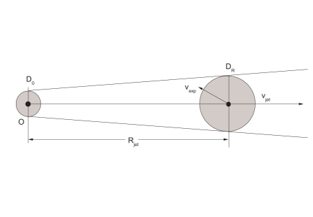
Figure 1: Sketch of axial cross section of geometry. $D_{\rm{0}}$ is the size of blob in the jet formation region around the central engine, and $D_{\rm{R}}$ is the size of blob at the position $R_{\rm{jet}}$ in the jet from the central engine.

The size $D_{\rm{R}}$ of a blob at the location $R_{\rm{jet}}$ can be constrained by the observed minimum timescale $\Delta t_{\rm{min}}^{\rm{ob}}$ of the variations from the blob, and we have

$$D_{\rm{R}}\leq\frac{\delta\Delta t_{\rm{min}}^{\rm{ob}}}{1+z}c,$$ (3)

where $\delta$ is the Doppler factor, $z$ is the redshift of source, and $c$ is the light speed. Combining equations (2) and (3), we have

$$D_{\rm{0}}\lesssim\frac{\delta\Delta t_{\rm{min}}^{\rm{ob}}}{1+z}c.$$ (4)

The inner radius of accretion disk is usually taken to be around the marginally stable orbit of disk surrounding the central black hole. The radius of marginally stable orbit of disk is

$$r_{\rm{ms}}=r_{\rm{g}}\{3+Z_{2}\mp[(3-Z_{1})(3+Z_{1}+2Z_{2})]^{1/2}\},$$ (5)

where $r_{\rm{g}}=GM_{\bullet}/c^{2}$ is the gravitational radius of black hole with a mass of $M_{\bullet}$, $Z_{1}\equiv 1+(1-j^{2})^{1/3}[(1+j)^{1/3}+(1-j)^{1/3}]$, and $Z_{2}\equiv(3j^{2}+Z_{1}^{2})^{1/2}$ (Bardeen et al., 1972). Here, $j=J/J_{\rm{max}}$ is the dimensionless spin parameter of black hole with the maximum possible angular momentum $J_{\rm{max}}=GM_{\rm{\bullet}}^{2}/c$ with $G$ being the gravitational constant. In the case of the prograde rotation, $r_{\rm{ms}}=6r_{\rm{g}}$ for $j=0$ and $r_{\rm{ms}}=r_{\rm{g}}$ for $j=1$. General relativistic magnetohydrodynamic simulations show that in the Schwarzchild case the jet-production region has a size around 14–16$r_{\rm{g}}$ (Meier et al., 2001), comparable to the diameter of the marginally stable orbit, $D_{\rm{ms}}=12r_{\rm{g}}$. In the Kerr case, the jet-production region must be of the order of the diameter of the ergosphere $D_{\rm{e}}=2r_{\rm{e}}=4r_{\rm{g}}$, where $r_{\rm{e}}$ is the equatorial boundary of the ergosphere (Meier et al., 2001). Thus the jet-production region span about from $D_{\rm{e}}$ to $D_{\rm{ms}}$ for $0\leq j\lesssim 1$, and then we take $D_{\rm{0}}=$4–12$r_{\rm{g}}$. From equation (4) and $D_{\rm{0}}=$4–12$r_{\rm{g}}$, we have

$$M_{\bullet}\lesssim 5.086\times 10^{4}\frac{\delta\Delta t_{\rm{min}}^{\rm{ob}}}{1+z}M_{\odot}\/\ \/\ (D_{\rm{0}}=D_{\rm{e}},\/\ j\sim 1),$$ (6a)

$$M_{\bullet}\lesssim 1.695\times 10^{4}\frac{\delta\Delta t_{\rm{min}}^{\rm{ob}}}{1+z}M_{\odot}\/\ \/\ (D_{\rm{0}}=D_{\rm{ms}},\/\ j=0),$$ (6b)

where $\Delta t_{\rm{min}}^{\rm{ob}}$ is in units of seconds. Equations (6a) and (6b) can be unified as

$$M_{\bullet}\lesssim 1.695{-}5.086\times 10^{4}\frac{\delta\Delta t_{\rm{min}}^{\rm{ob}}}{1+z}M_{\odot}$$ (7)

3 APPLICATIONS

The new method is applied to 32 blazars. These blazars have variability timescales of the order of hours with large variability amplitudes and a redshift range from 0.031 to 1.813. These timescales were reported in the literatures for the optical–X-ray–gamma-ray bands. The satellites detected GeV gamma rays from 29 out of 32 blazars. The details of these blazars are presented in Table 1. The minimum timescales of gamma rays are taken to be the doubling times of fluxes. The optical minimum timescales were reported in the literatures presented in column (6) of Table 1. The doubling times of X-ray fluxes are taken as the X-ray minimum timescales. These observed minimum timescales are listed in column (4), and their corresponding references are presented in column (6). The optical–$\gamma$-ray emission are mostly the Doppler boosted emission of jets for gamma-ray blazars (Ghisellini et al., 1998). A value of $\delta\sim$ 10 was adopted for GeV gamma-ray blazars (Ghisellini et al., 2010). We will take $\delta=10$ to estimate $M_{\bullet}$ with formula (7).

The Schwarzchild and Kerr black holes are considered in estimates of $M_{\bullet}$ from formula (7). The estimated black hole masses are denoted by $M^{\rm{Ker}}_{\rm{var}}$ and $M^{\rm{Sch}}_{\rm{var}}$ in columns (7) and (8) of Table 1, respectively. In the Schwarzchild case, $M^{\rm{Sch}}_{\rm{var}}$ spans from $10^{8.13}$ to $10^{9.68}$ $M_{\rm{\odot}}$. In the Kerr case, $M^{\rm{Ker}}_{\rm{var}}$ spans from $10^{8.61}$ to $10^{10.16}$ $M_{\rm{\odot}}$. We compared these estimated $M^{\rm{Sch}}_{\rm{var}}$ to those masses $M_{\rm{BH}}$ obtained with other methods reported in the literatures. In Figure 2 of $M_{\rm{BH}}$ versus $M^{\rm{Sch}}_{\rm{var}}$, there are five blazars below the line of $M_{\rm{var}}=M_{\rm{BH}}$. Because $M^{\rm{Sch}}_{\rm{var}}$ is only an upper limit of $M_{\bullet}$, the area below this line is not allowed for these blazars. When the central black holes are the Kerr ones, these upper limits of masses are increased by a factor 3, and four out of five blazars are moved into the area above the line of $M_{\rm{var}}=M_{\rm{BH}}$. Only 4C +38.41 is just below the line of $M_{\rm{var}}=M_{\rm{BH}}$. The populations of $M_{\bullet}$ in Figure 2 show that these $M_{\rm{var}}$ estimated from formula (7) are reasonable upper limits on $M_{\bullet}$ for blazars.

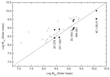
Figure 2: Black hole mass $M_{\rm{var}}$ versus $M_{\rm{BH}}$ estimated in other methods in the literatures. The solid line is $M_{\rm{var}}=M_{\rm{BH}}$. The triangles are $M_{\rm{var}}$ in the Schwarzchild case, and the solid circles are $M_{\rm{var}}$ in the Kerr case.

4 DISCUSSION AND CONCLUSIONS

Morini et al. (1986) thought X-ray emission to be produced very close to the inner engine in BL Lacertae object PKS 2155-304. Aharonian et al. (2007) limited the Doppler factor by the black hole mass and the variability timescale of very high energy gamma-ray flare of PKS 2155-304. Miller et al. (1989) reported the rapid variations on timescale as short as 1.5 hours for BL Lacertae in the optical flux, and the minimum timescale for the variations was used to place constraints on the size of the emitting region. They assumed that these variations were produced in the vicinity of a supermassive black hole, and then determined a black hole mass with the minimum timescale from a formula

$$M_{\bullet}=\frac{c^{3}\Delta t_{\rm{min}}^{\rm{ob}}}{6G(1+z)},$$ (8)

for the Schwarzchild black hole. At that time, they thought that relativistic beaming need not be invoked to account for the luminosity of this object. For the Kerr black hole, Xie et al. (2002c) deduced a formula from Abramowicz & Nobili (1982)

$$M_{\bullet}\lesssim 1.62\times 10^{4}\frac{\Delta t_{\rm{min}}^{\rm{ob}}}{1+z}M_{\odot},$$ (9)

which gives an upper limit on $M_{\bullet}$. These above two equations are based on assumption of accretion disk surrounding a supermassive black hole, and the optical flux variations are from the accretion disk. Obviously, these two formulae are applicable to estimate $M_{\bullet}$ for non-blazar-like AGNs or some AGNs with weaker blazar emission component in fluxes relative to accretion disk emission component. Considering the relativistic beaming effect, Xie et al. (2002c) deduced a new formula from formula (9)

$$M_{\bullet}\lesssim 1.62\times 10^{4}\frac{\delta\Delta t_{\rm{min}}^{\rm{ob}}}{1+z}M_{\odot}.$$ (10)

Formula (10) was applied to blazars, especially BL Lac objects (see Xie et al., 2002c, 2005b). In this paper, we proposed a sophisticated model to constrain the black hole masses using the rapid variations with large amplitudes for blazars. The model is suitable to constrain $M_{\bullet}$ in blazars using the minimum timescales of variations of the beamed emission from the relativistic jet. Formula (7) is the same as formula (10) in except of the coefficients in the right of formulae, but these two corresponding models are essentially different in their origins.

Spectral energy distributions of blazars consist of two broad peaks (e.g. Ghisellini et al., 1998). The first peak is produced by the synchrotron radiation processes of relativistic electrons in a relativistic jet. The second one is generally believed to come from the inverse Compton scattering processes of the same population of electrons. In general, the optical–gamma-ray emission are believed and/or assumed to be produced in the same region, simplified as a blob in simulating the spectral energy distributions of blazars. The coincidence of a gamma-ray flare with a dramatic change of optical polarization angle provides evidence for co-spatiality of optical and gamma-ray emission regions in 3C 279 (Abdo et al., 2010). Thus the timescales of the optical–X-ray–gamma-ray variations are used in formula (7). For this model, the blob size is assumed to increase linearly as it travels outward along the jet (see equation (1)). This linear growth assumption is only an approximation to the actual growth. The assumption will not change formula (2), and then don’t alter formula (7).

The errors associated with this method are quite high. Besides the poorly known details of the model itself, related to our ignorance of the exact distance from the black hole where the emission is produced, a large uncertainty is related to the value of the adopted Doppler factor. A value of $\delta=10$ is assumed, which may be in excess or short of the real value by at least a factor 3, resulting in a total uncertainty of at least an order of magnitude. In fact, it is possible for 32 blazars listed in Table 1. The Doppler factor $\delta$ can be estimated from the Lorentz factor and the viewing angle of jet adopted to model spectral energy distributions of bright Fermi blazars in Ghisellini et al. (2010). There are 21 Fermi blazars with new estimated $\delta$, and these new $\delta$ are from 13 to 28 with an average of 17. So, the upper limits of black hole masses are increased by a factor 1.3–2.8 when adopting these new $\delta$ for the 21 blazars. Thus the 29 Fermi blazars out of 32 blazars we employed will have a similar case for the upper limits of black hole masses. The adopted Doppler factor of $\delta=10$ may result in a large uncertainty with a factor 1.3–2.8 in the upper limits of $M_{\bullet}$. Another larger uncertainty with a factor 3.0 arises from the ignorance of spins of the central black holes in blazars (see formulae (6) and (7)). Thus the two large uncertainties will lead to errors of 3.9–8.4 in the upper limits of $M_{\bullet}$ estimated with this method for blazars.

In this paper, we proposed a sophisticated model to constrain the central black hole masses $M_{\bullet}$ with the observed minimum timescales $\Delta t^{\rm{ob}}_{\rm{min}}$ of variations in blazars. The size of a blob in the relativistic jet can be constrained with $\Delta t^{\rm{ob}}_{\rm{min}}$. The blob is assumed to be ejected from the jet-production region in the vicinity of black hole, and then to expand linearly as it travels outward along the jet. The model is applied to 32 blazars, out of which 29 blazars were detected in the GeV gamma-ray regime with the satellites. Their observed minimum timescales are on the order of hours with large variability amplitudes in the optical–X-ray–gamma-ray bands. In general, these $M_{\bullet}$ estimated from $\Delta t^{\rm{ob}}_{\rm{min}}$ by formula (7) are not inconsistent with those masses reported in the literatures. This indicates that this model is applicable to constrain $M_{\bullet}$ in the central engines of blazars. This model is more natural to connect $M_{\bullet}$ with $\Delta t^{\rm{ob}}_{\rm{min}}$ for blazars. Due to the ignorance of the black hole spins and the real Doppler factors, the uncertainty of the upper limits of masses will be about 3.9–8.4 in this method. The upper limits of masses will have uncertainty of 3.0 because the black hole spins are unknown for blazars, though we have the real Doppler factors rather than the adopted value of $\delta=10$ in this paper.

Table 1: Sample of blazars

Blazar name	$z$	Satelli.	$\Delta t_{\rm{min}}$	Band	Ref.	$M_{\rm{var}}^{\rm{Ker}}$	$M_{\rm{var}}^{\rm{Sch}}$	$M_{\rm{BH}}$	Ref.
(1)	(2)	(3)	(4)	(5)	(6)	(7)	(8)	(9)	(10)
3C 66A	0.444	EG,LAT	3.73	V	19	9.28	8.80	8.60	24
AO 0235+164	0.940	EG,LAT	4.74	R	9	10.16	9.68	9.30	24
RBS 0413	0.190	LAT	3.19	V	18	8.82	8.34	7.95	26
PKS 0420-01	0.916	EG,LAT	4.65	O	1	10.07	9.60	9.03	26
PKS 0537-441	0.894	EG,LAT	4.66	O	1	10.09	9.61	9.20	24
PKS 0548-322	0.069	None	3.14	R	21	8.82	8.34	8.15	22
S5 0716+71	0.300	EG,LAT	3.17	V	7	8.76	8.28	8.10	24
PKS 0735+17	0.424	EG,LAT	3.32	B	19	8.87	8.40	8.40	24
OJ 248	0.941	EG,LAT	3.65	R	20	9.07	8.59	8.41	27
OJ 287	0.306	EG,LAT	3.59	R	19	9.18	8.70	8.51	23
MrK 421	0.031	EG,LAT	3.26	TeV	4	8.95	8.48	8.29	22
4C +29.45	0.725	EG,LAT	4.40	O	17	9.87	9.39	8.56	27
W Com	0.102	LAT	3.58	V	16	9.24	8.77	7.40	24
4C+21.35	0.432	EG,LAT	3.92	GeV	3	9.47	8.99	8.20	24
3C 273	0.158	EG,LAT	4.33	V	11	9.97	9.50	9.39	25
3C 279	0.536	EG,LAT	3.38	V	19	8.90	8.42	8.43	26
PKS 1406-076	1.494	EG,LAT	4.76	R	14	10.07	9.59	9.40	24
PKS 1510-089	0.360	EG,LAT	3.39	R	20	8.96	8.49	8.31	27
AP Lib	0.049	LAT	2.95	O	1	8.64	8.16	8.09	22
PKS 1622-29	0.815	EG,LAT	4.14	GeV	8	9.59	9.11	9.10	24
4C +38.41	1.813	EG,LAT	4.76	GeV	2	10.02	9.54	10.10	24
3C 345	0.593	None	3.60	I	19	9.10	8.63	8.43	27
MrK 501	0.034	LAT	3.80	R	19	9.49	9.01	9.20	22
3C 371	0.051	LAT	3.38	X	12	9.06	8.59	8.50	22
PKS 2005-489	0.071	EG,LAT	3.84	X	5	9.52	9.04	9.00	26
OX 169	0.213	LAT	3.69	O	1	9.31	8.84	8.14	27
PKS 2155-304	0.116	EG,LAT	2.95	O	10	8.61	8.13	7.10	24
BL Lacertae	0.069	EG,LAT	3.30	B	15	8.98	8.50	8.23	26
CTA 102	1.037	EG,LAT	4.63	O	1	10.03	9.55	9.10	24
3C 454.3	0.859	EG,LAT	3.97	O	13	9.41	8.93	9.17	26
OY +091	0.190	None	3.30	B	15	8.93	8.45	8.62	26
1ES 2344+514	0.044	LAT	3.70	X	6	9.39	8.91	8.80	26

Note. — Column 1: Blazar names; Column 2: redshifts of objects; Column 3: The $\gamma$-ray satellites detected $\gamma$ rays from objects; Column 4: the minimum timescales of variations of objects; Column 5: the bands where the minimum timescales measured, B: the B band; V: the V band; R: the R band; I: the I band; O: the optical band; X: the X-ray band; Column 6: the references for columns 4 and 5; Column 7: the Kerr black hole masses estimated from equation (6a); Column 8: the Schwarzchild black hole masses estimated from equation (6b); Column 9: the black hole masses estimated with other methods in the literatures; Column 10: the references for column 9.

References: (1) Bassani et al. 1983; (2) Fan et al. 1999; (3) Foschili et al. 2011; (4) Gaidos et al. 1996; (5) Giommi et al. 1990; (6) Giommi et al. 2000; (7) Gupta et al. 2009; (8) Mattox et al. 1997; (9) Moles et al. 1985; (10) Paltani et al. 1997; (11) Rani et al. 2011; (12) Staubert et al. 1986; (13) Villata et al. 1997; (14) Wagner et al. 1995; (15) Xie et al. 1990; (16) Xie et al. 1991a; (17) Xie et al. 1991b; (18) Xie et al. 1992; (19) Xie et al. 1999; (20) Xie et al. 2001; (21) Xie et al. 2002a; (22) Barth et al. 2003; (23) Liu & Wu 2002; (24) Liang & Liu 2003; (25) Paltani & Türler 2005; (26) Woo & Urry 2002; (27) Xie et al. 2005a.

References

- Abdo et al. (2010) Abdo, A. A., Ackermann, M., Ajello, M., et al. 2010, Natur, 463, 919
- Abramowicz & Nobili (1982) Abramowicz, M. A., & Nobili, L. 1982, Natur, 300, 506
- Aharonian et al. (2007) Aharonian, F., Akhperjanian, A. G., Bazer-Bachi, A. R., et al. 2007, ApJ, 664, L71
- Arshakian et al. (2010) Arshakian, T. G., León-Tavares, J., Lobanov, A. P., et al. 2010, MNRAS, 401, 1231
- Bardeen et al. (1972) Bardeen, J. M., Press, W. H., & Teukolsky, S. A. 1972, ApJ, 178, 347
- Barth et al. (2003) Barth, A. J., Ho, L. C., & Sargent, W. L. W. 2003, ApJ, 583, 134
- Bassani et al. (1983) Bassani, L., Dean, A. J., & Sembay, S. 1983, A&A, 125, 52
- Blandford & Payne (1982) Blandford, R. D., & Payne, D. G. 1982, MNRAS, 199, 883
- Blandford & Rees (1978) Blandford, R. D., & Rees, M. J. 1978, in Pittsburgh Conf. on BL Lac Objects, ed. A. M. Wolfe (Pittsburgh, PA: Univ. Pittsburgh Press), 328
- Blandford & Znajek (1977) Blandford, R. D., & Znajek, R. 1977, MNRAS, 179, 433
- Chatterjee et al. (2009) Chatterjee, R., Marscher, A. P., Jorstad, S. G., et al. 2009, ApJ, 704, 1689
- Chatterjee et al. (2011) Chatterjee, R., Marscher, A. P., Jorstad, S. G., et al. 2011, ApJ, 734, 43
- Fan et al. (1999) Fan, J. H., Xie, G. Z., & Bacon, R. 1999, A&AS, 136, 13
- Foschili et al. (2011) Foschili, L., Ghisellini, G., Tavecchio, F., Bonnoli, G., & Stamerra, A. 2011, A&A, 530, A77
- Gaidos et al. (1996) Gaidos, J. A., Akerlof, C. W., Biller, S. et al. 1996, Natur, 383, 319
- Ghisellini et al. (1998) Ghisellini, G., Celotti, A., Fossati, G., Maraschi, L., & Comastri, A. 1998, MNRAS, 301, 451
- Ghisellini et al. (2010) Ghisellini, G., Tavecchio, F., Foschini, L., et al. 2010, MNRAS, 402, 497
- Giommi et al. (1990) Giommi, P., Barr, P., Pollock, A. M. T., Garilli, B., & Maccagni, D. 1990, ApJ, 356, 432
- Giommi et al. (2000) Giommi, P., Padovani, P., & Perlman, E. 2000, MNRAS, 317, 743
- Gupta et al. (2009) Gupta, A. C., Srivastava, A. K., & Wiita, P. J. 2009, ApJ, 690, 216
- Liang & Liu (2003) Liang, E. W. & Liu, H. T. 2003, MNRAS, 340, 632
- Liu & Wu (2002) Liu, F. K. & Wu, X. B. 2002, A&A, 388, L48
- Marscher et al. (2002) Marscher, A. P., Jorstad, S. G., Gómez, J. L., et al. 2002, Natur, 417, 625
- Mattox et al. (1997) Mattox, J. R., Wagner, S. J., Malkan, M., et al. 1997, ApJ, 476, 692
- Meier et al. (2001) Meier, D. L., Koide, S., & Uchida, Y. 2001, Sci, 291, 84
- Miller et al. (1989) Miller, H. R., Carini, M. T., & Goodrich, B. D. 1989, Natur, 337, 627
- Moles et al. (1985) Moles, M., Garcia-Pelayo, J. M., Masegosa, J., & Aparicio, A. 1985, ApJS, 58, 255
- Morini et al. (1986) Morini M., Chiappetti, L., Maccagni, D., et al. 1986, ApJ, 306, L71
- Paltani et al. (1997) Paltani, S., Courvoisier, T. J.-L., Blecha, A., & Bratschi, P. 1997, A&A, 327, 539
- Paltani & Türler (2005) Paltani, S. & Türler, M. 2005, A&A, 435, 811
- Penrose (1969) Penrose, R. 1969, NCimR, 1, 252
- Rani et al. (2011) Rani, B., Gupta, A. C., Joshi, U. C., Ganesh, S., & Wiita, P. J. 2011, MNRAS, 413, 2157
- Staubert et al. (1986) Staubert, R., Brunner, H., & Worrall, D. M. 1986, ApJ, 310, 694
- Urry & Padovani (1995) Urry, C. M., & Padovani, P. 1995, PASP, 107, 803
- Villata et al. (1997) Villata, M., Raiteri, C. M., Ghisellini, G., et al. 1997, A&AS, 121, 119
- Wagner et al. (1995) Wagner, S. J., Mattox, J. R., Hopp, U. et al. 1995, ApJ, 454, L97
- Wagner & Witzel (1995) Wagner, S. J., & Witzel, A. 1995, ARA&A, 33, 163
- Woo & Urry (2002) Woo, J. H. & Urry, C. M. 2002, ApJ, 579, 530
- Xie et al. (1988) Xie, G. Z., Li, K. H., Zhou, Y., et al. 1988, AJ, 96, 24
- Xie et al. (1990) Xie, G. Z., Li, K. H., Cheng, F. Z., et al. 1990, A&A, 229, 329
- Xie et al. (1991a) Xie, G. Z., Li, K. H., Cheng, F. Z., et al. 1991a, A&AS, 87, 461
- Xie et al. (1991b) Xie, G. Z., Liu, F. K., Liu, B. F., et al. 1991b, AJ, 101, 71
- Xie et al. (1992) Xie, G. Z., Li, K. H., Liu, F. K., et al. 1992, ApJS, 80, 683
- Xie et al. (1999) Xie, G. Z., Li, K. H., Zhang, X., Bai, J. M., & Liu, W. W. 1999, ApJ, 522, 846
- Xie et al. (2001) Xie, G. Z., Li, K. H., Bai, J. M., et al. 2001, ApJ, 548, 200
- Xie et al. (2002a) Xie, G. Z., Zhou, S. B., Dai, B. Z., et al. 2002a, MNRAS, 329, 689
- Xie et al. (2002b) Xie, G. Z., Liang, E. W., Zhou, S. B., et al. 2002b, MNRAS, 334, 459
- Xie et al. (2002c) Xie, G. Z., Liang, E. W., Xie, Z. H., & Dai, B. Z. 2002c, AJ, 123, 2352
- Xie et al. (2005a) Xie, G. Z., Liu, H. T., Cha, G. W., et al. 2005a, AJ, 130, 2506
- Xie et al. (2005b) Xie, G. Z., Ma, L., Zhou, S. B., Chen, L. E., & Xie, Z. H. 2005b, PASJ, 57, 183