Interaction of hopfions of charge 1 and 2 from product ansatz

Abstract

We continue the discussion on the interaction energy of the axially symmetric Hopfions evaluated directly from the product anzsatz. The Hopfions are given by the projection of Skyrme model solutions onto the coset space SU(2)/U(1). Our results show that if the separation between the constituents is not small, the product ansatz can be considered as a good approximation to the general pattern of Hopfions interaction both in repulsive and attractive channel.

1 Introduction

Topological and non-topological solitons appear in many non-linear field models in various contexts. Since the appearance of the soliton solutions on the theoretical scene in the 1970s, it has become evident that they play a prominent role in classical and quantum field theory. These spatially localized non-perturbative stable field configurations are natural in a wide variety of physical systems [1].

The Faddeev-Skyrme model in $d=3+1$ is a modified scalar $O(3)$-sigma model with a quartic in derivatives term [2]. The structure of the Lagrangian of this model is similar with the original Skyrme model [3], whose solitons are posited to model atomic nuclei, however the topological properties of the corresponding solitions, Hopfions and Skyrmions, are very different. It was shown that soliton solutions of the Faddeev-Skyrme model should be not just closed flux-tubes of the fields but knotted field configurations.

The first explicit non-trivial Hopfion solutions were constructed numerically by Battye and Sutcliffe [16] who found the trefoil knotted solution in the Faddeev-Skyrme model. Consequent analyses revealed a very rich structure of the Hopfion states [4, 5]. The subsequent development have revealed a plethora of such topological solutions with a non-trivial value of the Hopf invariant, which play a prominent role in the modern physics [6], chemistry [7] and biology [8]. A number of different models which describe topologically stable knots associated with the first Hopf map $S^{3}\to S^{2}$ are known in different contexts. It was argued, for example, that a system of two coupled Bose condensates may support Hopfion-like solutions [9], or that glueball configurations in QCD may be treated as Hopfions.

Note that most of the investigations of the Skyrmions and Hopfions mainly focus on the search for classical static solutions. Indeed, since in both models these configurations do not saturate the topological bound, the powerful technique of the moduli space approximation cannot be directly applied to analyse the low-energy dynamics of the solitons. Therefore in order to investigate the process of interaction between these solutions one has to implement rather advanced numerical methods.

Interestingly, the numerical simulations of the head-on collision of the charge one Skyrmions still reveal the well known pattern of the $\pi/2$ scattering through the intermediate axially-symmetric charge two Skyrmion [10], which is typical for self-dual configurations like BPS monopoles [1]. However recent attempt to model the Hopfion dynamics [14] failed to find the channel of right-angle scattering in head-on collisions of the charge one solitons.

Another approach to the problem of interaction between the stringlike solitons of the Faddeev-Skyrme model is to consider the asymptotic fields of the Hopfion of degree one, which corresponds to a doublet of orthogonal dipoles [12, 13]. Investigating this limit Ward predicted existence of three attractive channels in the interaction of the Hopfions with different orientation [13].

In his pioneering paper [3] Skyrme suggested to implement so-called product ansatz to approximate a composite configuration of well-separated individual Skyrmions. The ansatz is constructed by the multiplication of the Skyrmion matrix-valued fields. Note that besides the rational map ansatz [15] it can be applied to produce an initial multi-Skyrmion configuration for consequent numerical calculations in a sector of given degree [16]. Evidently, the same approach can be used to model the configuration of well separated static Hopfions of degree one to approximate various multicomponent configurations.

Recently we discussed the relation between the solutions of the Skyrme model of lower degree and the corresponding axially symmetric Hopfions which is given by the projection onto the coset space $SU(2)/U(1)$ [11]. Using this approach we made use of the product ansatz of two well-separated single Hopfions and confirmed that the product ansatz correctly reproduces the channels of interaction between them. In this paper we briefly describe the relation between the solutions of the Skyrme model of lower degrees and the corresponding axially symmetric Hopfions which is given by the projection onto the coset space, adding here new and updated results of the numerical evaluation of the corresponding interaction energy of the Hopfions.

2 The model

The Faddeev-Skyrme model in 3+1 dimensions with metric $(+,-,-,-)$ is defined by the Lagrangian

$${\cal L}=\frac{1}{32\pi^{2}}\left(\partial_{\mu}\phi^{a}\partial^{\mu}\phi^{a}-\frac{1}{4}(\varepsilon_{abc}\phi^{a}\partial_{\mu}\phi^{b}\partial_{\nu}\phi^{c})^{2}\right)\,,$$ (1)

where $\phi^{a}=(\phi^{1},\phi^{2},\phi^{3})$ denotes a triplet of scalar real fields which satisfy the constraint $|\phi^{a}|^{2}=1$. The finite energy configurations approach a constant value at spatial infinity, which we choose to be $\phi^{a}(\infty)=(0,0,1)$. For fields $\boldsymbol{\phi}(\mathbf{x})$ with this property the domain of definition, i. e. 3D Euclidian space, is equivalent to $S^{3}$ sphere and $\boldsymbol{\phi}(\mathbf{x})$ defines the map $S^{3}\to S^{2}$. It is well known that these maps are characterized by Hopf invariants $Q=\pi_{3}(S^{2})=\mathbb{Z}$, where the target space $S^{2}$ by construction is the coset space $SU(2)/U(1)$.

Any coset space element $\mathbf{H}$ can be projected from generic $SU(2)$ group element $\mathbf{U}$. In circular coordinate system the projection takes the form

$$\mathbf{H}=2\sum_{a}(-1)^{a}\tau_{a}\phi_{-a}=2\mathbf{U}\tau_{0}\mathbf{U}^{\dagger}\,,$$ (2)

where the Pauli matrices $(\tau_{1},\tau_{0},\tau_{-1})$ satisfy relation

$$\tau_{a}\tau_{b}=\frac{1}{4}(-1)^{a}\delta_{a,-b}\mathbf{1}-\frac{1}{\sqrt{2}}\left[\begin{array}[]{ccc}1&1&1\\ a&b&c\end{array}\right]\tau_{c}.$$ (3)

The symbol in square brackets denotes the Clebsch-Gordon coefficient. Then the Lagrangian (1) can be rewritten in terms of coset space elements $\mathbf{H}$,

$$\begin{split}{\cal L}=&\frac{1}{64\pi^{2}}\Bigl{(}\mathop{\mathrm{Tr}}\big{\{}\partial_{\mu}\mathbf{H}\partial^{\mu}\mathbf{H}\big{\}}\\ &+\frac{1}{16}\mathop{\mathrm{Tr}}\big{\{}\bigl{[}\partial_{\mu}\mathbf{H},\partial_{\nu}\mathbf{H}\bigr{]}\bigl{[}\partial^{\mu}\mathbf{H},\partial^{\nu}\mathbf{H}\bigr{]}\big{\}}\Bigr{)}\,.\end{split}$$ (4)

The difference between the Skyrmions and Hopfions is that in the latter case the dimensions of the domain space and the target space are not the same. The topological charge of the Hopfions, which meaning is the linking number in the domain space [2], is not defined locally.

There have been many investigations of the solutions of the model (1) for higher degree $Q$ [12, 5, 16, 4]. Here we consider projections of general rational map Skyrmion ansatz, however numerical results of interaction potential is presented only for axially symmetric configurations of lower degrees $Q=1,2$ which are conventionally labeled as ${\cal A}_{1,1}$ and ${\cal A}_{2,1}$ [5].

An rational map approximation to these solutions can be constructed via Hopf projection of the corresponding Skyrmion configurations [17]. Recall that the rational map ansatz [18] is an approximation to the ground state solution of the Skyrme model, which for baryon number $B\geq 1$ takes the following form:

$$U_{R}(\mathbf{r})=\exp(2\mathrm{i}\,\hat{n}^{a}_{R}\hat{\tau}_{a}F(r))\,.$$ (5)

The unit vector $\hat{\mathbf{n}}_{R}$ is defined in terms of a rational complex function $R(z)=p(z)/q(z)$, where $p(z)$ and $q(z)$ are polynomials of complex variable $z$ of degree at most $N$, and $p$ and $q$ have no common roots. In Cartesian coordinates the components of $\hat{{\mathbf{n}}}_{R}$ then can be written as

$$\hat{{\mathbf{n}}}_{R}=\frac{1}{1+|R|^{2}}\{2\Re(R),2\Im(R),1-|R|^{2}\}\,.$$ (6)

Parametrizing the complex variable $z=\tan(\theta/2)\mathrm{e}^{\mathrm{i}\varphi}$ by polar and azimuthal angles $\theta$ and $\varphi$ we can find explicit expression for any given rational function $R$. In particular, for baryon charge $B=1$ we take $R(z)=z$, which gives

$$\hat{{\mathbf{n}}}_{1}=\hat{{\mathbf{r}}}=\{\bigl{(}\mathrm{e}^{-\mathrm{i}\varphi}\sin\theta\bigr{)}/\sqrt{2},\cos\theta,\bigl{(}-\mathrm{e}^{\mathrm{i}\varphi}\sin\theta\bigr{)}/\sqrt{2}\}\,.$$ (7)

We also implement the circular coordinates $\hat{n}_{\pm 1}=\mp\frac{1}{\sqrt{2}}\bigl{(}\hat{n}^{1}\pm\mathrm{i}\hat{n}^{2}\bigr{)}$ and $\hat{n}_{0}=\hat{n}^{3}$, where $\hat{n}^{i}$ denotes the Cartesian components of the unit vector (6). It is known that simple choice $R(z)=z$ yields an exact solution of the model.

For $B=2$ Skyrmion the lowest energy rational map approximation is given by the choice $R(z)=z^{2}$, or explicitly in circular coordinates

$$\hat{{\mathbf{n}}}_{2}=\{\frac{\mathrm{e}^{-2\mathrm{i}\varphi}\sin^{2}\theta}{\sqrt{2}\bigl{(}1+\cos^{2}\theta\bigr{)}},\frac{2\cos\theta}{1+\cos^{2}\theta},\frac{-\mathrm{e}^{2\mathrm{i}\varphi}\sin^{2}\theta}{\sqrt{2}\bigl{(}1+\cos^{2}\theta\bigr{)}}\}\,.$$ (8)

For higher baryon numbers rational map approximations are also well known [1], thought the correspondence between them and exact numerical results is getting worse as baryon number $B$ increases. Note, that in the topologically trivial sector $B=0$ we may take $\hat{{\mathbf{n}}}_{0}=\{1/\sqrt{2},0,-1/\sqrt{2}\}$, which we used to test the product ansatz approximation.

Note that the Skyrme model can be consistently reduced [17] to Faddeev-Skyrme model by restricting SU(2) Lie algebra currents $\mathbf{U}^{\dagger}\partial_{\mu}\mathbf{U}$ to coset representation (2). This means that Faddeev-Skyrme fields configurations with Hopf charge $Q$ corresponds to Skyrme field with the baryon number $B$. Therefore the projection of rational map ansatz (5) yields the rational map approximation of the Hopf charge of the same degree $Q=N$. Moreover, the usual profile function $F(r)$ of Skyrme model, which is a monotonically decreasing function satisfying boundary conditions $F(0)=\pi,~{}~{}F(\infty)=0$, can be used. This projection produces the Hopfion configuration of degree one with mass $1.232$.

As usual, we denote the ${\cal A}_{1,1}$ configuration as $\mathbf{H}_{1}$ which is a projection of the Skyrmion matrix valued field $\mathbf{U}_{R=z}$, i.e.

$$\mathbf{H}_{1}(\mathbf{r})=2\mathbf{U}_{R=z}(\mathbf{r})\tau_{0}\mathbf{U}_{R=z}^{\dagger}(\mathbf{r})\,,$$ (9)

where $\mathbf{U}_{R=z}(\mathbf{r})$ is the usual spherically symmetric hedgehog ansatz parametrised by rational map (5) with $R(z)=z$ and $\hat{\mathbf{n}}_{R}$ is defined by eq. (7). It should be noted, that although the ansatz (5) for $B=1$ is spherically symmetric, the corresponding Hopfion of degree $Q=1$ does not possess the spherical symmetry. The projection breaks it down to axial symmetry ${\cal A}_{1,1}$ [16].

The position curve of Hopfion is chosen to be the curve of the preimages of the point $(0,0,-1)$ which is the antipodal to the vacuum $(0,0,1)$. For the simplest ${\cal A}_{1,1}$ Hopfion this is a circle of radius $F(r_{c})=\pi/2$, with numerical value $r_{c}=0.8763$ in the $x-y$ plane. Small deviations $F(r)=F(r_{0})+\epsilon$ then define the tube around the position curve where $\vartheta\approx\pi/2$ and $\varphi=[0,2\pi)$. The same is true for $R(z)=z^{2}$ or ${\cal A}_{2,1}$ configuration, except that point on tube rotates twice when angle $\varphi$ changes from $0$ to $2\pi$ and the radius of circle being slightly large, $r_{c}=1.299$.

For single Hopfion we can also rotate the points on the tube about the vertical $x_{3}$ axis by applying rotation transform via the $SU(2)$ matrix

$$\mathbf{H}\rightarrow D(\alpha)\mathbf{H}D(-\alpha)\,.$$ (10)

This global transformation corresponds to the symmetry of the Lagrangian (4).

Let us now consider two Hopfions of arbitrary charges which are placed at the points $\mathbf{R}/2$ and $-\mathbf{R}/2$ and separated by a distance $R$, as shown in Figure 1. There the polar angle $\Theta$ corresponds to the orientation of the Hopfions with respect to the $z$-axis. Note that for $R=z$ the pattern of interaction between the charge one Hopfions is invariant with respect to the spacial rotations of the system around the $z$-axis by an azimuthal angle $\Phi$. This additional symmetry does not appear for higher maps, e.g. for $R=z^{2}$.

Figure 1: Geometry of the system of two interacting Hopfions $h_{1}$ and $h_{2}$, which are located at the points $\mathbf{R}/2$ and $-\mathbf{R}/2$ (indicated by arrows), respectively. The dot position on hopfion core illustrates the hopfion orientation (oposite phase case $\Delta\alpha=\pi$ is shown here).

First, we suppose that both separated Hopfions are of positive charges and they are in phase, i.e. for example, rotation matrices $D(\alpha)$ in (10) are identities for both Hopfions. More strictly, the definition ”in phase” only means that the difference between the angles of rotations of individual Hopfions is zero, $\Delta\alpha=0$.

Then the system of two hopfions can be approximated by the product ansatz

$$\mathbf{H}_{N}^{\Delta\alpha=0}(\mathbf{r})=2\mathbf{U}_{R^{\prime}}(\mathbf{r}^{\prime})\mathbf{U}_{R^{\prime\prime}}(\mathbf{r}^{\prime\prime})\tau_{0}\mathbf{U}_{R^{\prime\prime}}^{\dagger}(\mathbf{r}^{\prime\prime})\mathbf{U}_{R^{\prime}}^{\dagger}(\mathbf{r}^{\prime})\,,$$ (11)

where $\mathbf{r}^{\prime}=\mathbf{r}+\mathbf{R}/2$ and $\mathbf{r}^{\prime\prime}=\mathbf{r}-\mathbf{R}/2$ and $N$ denotes the sum of degrees of rational maps $R^{\prime}$ and ${R^{\prime\prime}}$. Fields of both Hopfions in (11) at the spacial boundary tend to the same asymptotics $(0,0,1)$. Also note, that in the constituent system (11) of two Hopfions, contrary to the single Hopfion case, the transformation (10) of one of the Hopfions $\mathbf{H}$ do not leave the Lagrangian (4) invariant, it becomes a function of the relative phase $\Delta\alpha$.

In addition to the ansatz (11) we can as well consider the system of two separated Hopfions, when one of them is relatively rotated by arbitrary angle $\alpha$. Here, hovewer, we only restrict ourself to the relative phase $\Delta\alpha=\pi$, i.e., to the case when Hopfions have opposite phases. Taking one of rotation matrix $D(0)$ to be identity matrix and the other $D(\pi)=2\tau_{0}$, we can express this system in terms of the matrices $\mathbf{U}_{R^{\prime}}$ and $\mathbf{U}_{R^{\prime\prime}}$, thus the corresponding product ansatz is now different from (11):

$$\mathbf{H}_{N}^{\Delta\alpha=\pi}(\mathbf{r})=8\mathbf{U}_{R^{\prime}}(\mathbf{r}^{\prime})\tau_{0}\mathbf{U}_{R^{\prime\prime}}(\mathbf{r}^{\prime\prime})\tau_{0}\mathbf{U}_{R^{\prime\prime}}^{\dagger}(\mathbf{r}^{\prime\prime})\tau_{0}\mathbf{U}_{R^{\prime}}^{\dagger}(\mathbf{r}^{\prime})\,,$$ (12)

The product ansatz approximations (11) and (12) ensures the conservation of the total topological charge for any separation $R$ and space orientation of the constituents. Note, however, that in the case of different rational maps ${R^{\prime}}\neq R^{\prime\prime}$, for example, $z$ and $z^{2}$, which are considered below, their order in (11) and (12) is important. The different ordering yields different numerical results for small separation distances $R$, because the chiral angles for $F_{R^{\prime}}(r^{\prime})$ and $F_{R^{\prime\prime}}(r^{\prime\prime})$ differ. This problem will be investigated in more detail elsewhere.

Substitution of product ansatzes (11) and (12) into Lagrangian (4) yields energy densities of both configurations in terms of components of the position vectors $r_{i}^{\prime}$ and $r_{j}^{\prime\prime}$ (cf Figure 1).

Let us express these components via Hopfion’s position coordinates $R,\Theta,\Phi$ and the spherical coordinates $r,\theta,\varphi$, then the numerical integration of the corresponding local densities over the variables $\varphi,\vartheta$ and $r$ yields the total energy (mass) of the system and its topological charge. The density of the latter quantity in circular coordinates is given by the trace formula

$$\begin{split}{\cal Q}(\mathbf{r}^{\prime},\mathbf{r}^{\prime\prime})&=\mathrm{i}\sqrt{2}(-1)^{a+b}\left[\begin{array}[]{ccc}1&1&1\\ a&b&a+b\end{array}\right]\\ &\times\mathop{\mathrm{Tr}}\Bigl{(}\nabla_{a}\bigl{(}\mathbf{U}_{R^{\prime}}(\mathbf{r}^{\prime})\mathbf{U}_{R^{\prime\prime}}(\mathbf{r}^{\prime\prime})\bigr{)}\mathbf{U}_{R^{\prime\prime}}^{\dagger}(\mathbf{r}^{\prime\prime})\mathbf{U}_{R^{\prime}}^{\dagger}(\mathbf{r}^{\prime})\\ &\times\nabla_{b}\bigl{(}\mathbf{U}_{R^{\prime}}(\mathbf{r}^{\prime})\mathbf{U}_{R^{\prime\prime}}(\mathbf{r}^{\prime\prime})\bigr{)}\mathbf{U}_{R^{\prime\prime}}^{\dagger}(\mathbf{r}^{\prime\prime})\mathbf{U}_{R^{\prime}}^{\dagger}(\mathbf{r}^{\prime})\\ &\times\nabla_{-a-b}\bigl{(}\mathbf{U}_{R^{\prime}}(\mathbf{r}^{\prime})\mathbf{U}_{R^{\prime\prime}}(\mathbf{r}^{\prime\prime})\bigr{)}\mathbf{U}_{R^{\prime\prime}}^{\dagger}(\mathbf{r}^{\prime\prime})\mathbf{U}_{R^{\prime}}^{\dagger}(\mathbf{r}^{\prime})\Bigr{)}\,.\end{split}$$

We used the evaluation of the total topological charge of the configuration (for different values of the separation parameter $R$) as a correctness test of our numerical computations. The potential energy of interaction between two Hopfions of degree one and two is evaluated by subtracting of the corresponding masses of single Hopfions, i.e. $m_{(R^{\prime}=z)}=1.2314$ and $m_{(R^{\prime\prime}=z^{2})}=2.079503$, from the integrated density (4) evaluated on the configurations (11) and (12), respectively.

3 Numerical results

a)

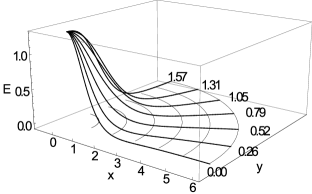
Figure 2: The evaluated interaction energy of the $\Delta\alpha=0$ (in phase), product $Q=1+1$ ansatz Hopfions as a function of the orientation parameters $R$ and $\Theta$.

Evaluation of the total topological charge and the energy of the product ansatz configuration requires numerical integration. In particularly, for each given set of fixed values of the orientation parameters $R$, $\Theta$ and $\Phi$, the integration of the energy density and Hopfion charge density (2) over three components of the Hopfion field yields, correspondingly, the strength of the interaction energy of the Hopfions and the topological charge of the configuration.

We have performed calculations with different values of the parameters $R$, $\Theta$ and $\Phi$ for system of two product ansatz $Q=1$ Hopfions [19] (figures 2 and 3), system consisting of $Q=1$ and $Q=2$ Hopfions (figures 4 – 7), and for two $Q=2$ Hopfions (figures 8 – 10). All figures demonstrate the integrated interaction energy as a function of the orientation parameters for the ”in phase” Hopfions and the Hopfions with oposite phases. Clearly, we can expect our approximation of the interaction energy in the system of two separated Hopfions will be reliable only if the separation parameter $R$ is larger than the sum of cores of the constituents $r_{c}$.

Our results show that system of two $Q=1$ Hopfions approximated via the product ansatzes (11) and (12) is in complete agreement with interaction pattern of the Hopfions based on the simplified dipole-dipole approximation [13]. It should be noted that there was a minor mistake in our evaluation of the weight factors of the $L_{2}$ and $L_{4}$ terms in the effective Largangian presented previously in [19]. Fortunately, this mistake may affect the results only in the case of small values of the separation parameter $R$, i.e. when the Hopfions cannot be considered as individual constituents, thus all predictions of [19] remain valid.

In particulary, when the Hopfions are in phase and $\Theta=0$, which corresponds to Channel A in [13], there is a shallow ($-0.05$ at $R\approx 2.6$) attractive window for separations $R$ large than $1.8$, as can be seen from Fig. 2. Evidently, this attractive channel is very narrow because the potential of interaction quickly becomes repulsive as the value of $\Theta$ increases.

a)

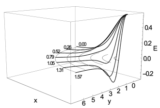
Figure 3: The interaction energy of the $\Delta\alpha=\pi$ (opposite phases), product $Q=1+1$ ansatz Hopfions as a function of the orientation parameters $R$ and $\Theta$.

When Hopfions are in side by side position, $\Theta=\pi/2$, the interaction potential is always repulsive as is shown in Fig. 2. The interaction strength for other orientations of the Hopfions is represented by a surface in Fig. 2.

Quite different pattern of interaction, however, occurs between the opposite phase ${\cal A}_{1,1}$ Hopfions, which is depicted in Fig. 3. In contrast with Fig. 2 in the Channel A ($\Theta=0$) the interaction is always repulsive for all values of the separation distance $R$.

However, in the Channel B [13] ($\Theta=\pi/2$) the interaction energy has relatively large negative value ($-0.266$ at $R=1.6$) at the separation of about two cores $r_{c}=0.8763$ (the interaction is attractive till $R\approx 1.1$) and then gradually decreases to zero as separation between the Hopfions increases, Fig. 3. The repulsive behaviour changes to attraction at $\Theta\approx\pi/3$, it approaches maximum as $\Theta=\pi/2$. For the Hopfions which are in opposite phases, this pattern is presented in Fig. 3 where we plotted the interaction energy as function of the orientation parameters $R$ and $\Theta$. Qualitatively, the pattern of interaction between the Hopfions both in the Channel A and in the Channel B, is in a good agreement with results of full 3d numerical simulations of the Hopfions dynamics [14].

Unfortunately there is no similar 3d simulation data neither for ${\cal A}_{1,1}$, ${\cal A}_{2,1}$ configurations, ${\cal A}_{1,1}$ and ${\cal A}_{2,1}$ (figures 4 – 7), nor for two ${\cal A}_{2,1}$ Hopfions (figures 8 – 10) interactions. Below we consider the product ansatz approximation of these systems.

It is clear, that in these cases the configuration are less symmetric and the interaction profiles are more involved, generally they depend on the value of the azimuthal angle $\Phi$. In the case of ${\cal A}_{1,1}$ and ${\cal A}_{2,1}$ Hopfion interaction, which in short will be denoted as $1+2$, the shape of interaction energy isosurface for fixed values of the angles $\Phi=0$ and $\Phi=\pi/2$ are shown in Figs 4 (in phase) and 6 (the case of opposite phases). We see that contrary to $1+1$ case strongest attraction (interaction energy minimum is $-0.168$ at $R\approx 2.2$) now is observed for Hopfions in phase (Fig. 4), whereas for the oppositely oriented Hopfions (cf Fig 6) there is only a shallow minimum ($-0.014$ at $R\approx 2.4$) for some narrow interval of values of the orientation angle $\Theta$.

In the case of interaction between two Hopfions ${\cal A}_{2,1}$ ($2+2$ case), strongest attraction channel occurs again for the Hopfions with opposite phase, similar to the interaction pattern in the $1+1$ case. The interaction energy minimum, however, becomes shallower with increasing of the Hopfion charges. In particular, in the $2+2$ case the interaction energy approaches its minimal value $-0.165$ at $R\approx 1.4$, compared to $-0.266$ at $R=1.6$ in the $1+1$ case.

In the case of the $1+2$ system the interaction energy, in general, has nontrivial dependency on the value of the azimuthal angle $\Phi$, as shown in Fig 5. In a particular case $\Theta=0$ (one Hopfion is above the other), the system possesses the axial symmetry and the dependency of the interaction potential on the value of $\Phi$ is trivial.

However for other values of polar angle$\Theta$, for example for $\Theta=\pi/2$ (the Hopfions are in the horizontal plane), this dependency can be evidently seen. Note that in the cases of the $1+1$ and $2+2$ systems there is no dependency of the interaction energy on the value of the azimuthal orientation angle $\Phi$.

In our consideration of the interaction between the Hopfions we mainly concentrate ourselves on the description of possible attractive channels. Note that all the possible repulsive channels are illustrated in Figs. 2–10, thus we may also draw some conclusions about the repulsion strength between the Hopfions for different orientation angles and separation distance $R$.

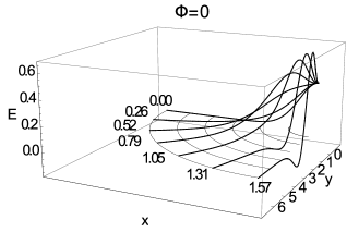
a) b)

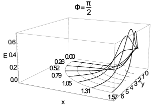
Figure 4: The evaluated interaction energy of the $\Delta\alpha=0$ (in phase), $Q=1+2$ product ansatz Hopfions is plotted as function of the orientation parameters $R$ and $\Theta$ for fixed angles $\Phi=0$ a) and $\Phi=\pi/2$ b).

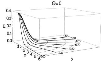
a) b)

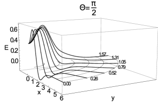
Figure 5: The evaluated interaction energy of the $\Delta\alpha=0$ (in phase), $Q=1+2$ product ansatz Hopfions as a function of the orientation parameters $R$ and $\Phi$ for fixed angles $\Theta=0$ a) and $\Theta=\pi/2$ b).

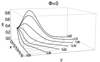
a) b)

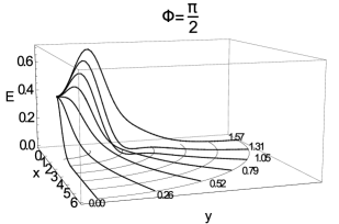
Figure 6: The evaluated interaction energy of the $\Delta\alpha=\pi$ (opposite phase), $Q=1+2$ product ansatz Hopfions as a function of the orientation parameters $R$ and $\Theta$ for fixed angles $\Phi=0$ a) and $\Phi=\pi/2$ b).

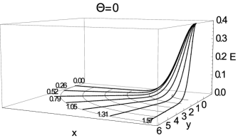
a) b)

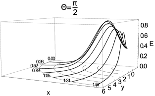
Figure 7: The evaluated interaction energy of the $\Delta\alpha=\pi$ (opposite phase), $Q=1+2$ product ansatz Hopfions as a function of the orientation parameters $R$ and $\Phi$ for fixed angles $\Theta=0$ a) and $\Theta=\pi/2$ b).

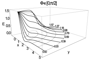
a) b)

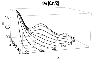
Figure 8: The evaluated interaction energy of the $\Delta\alpha=0$ (in phase) a) and of the $\Delta\alpha=\pi$ (opposite phase) b) of $Q=2+2$ product ansatz Hopfions as a function of the orientation parameters $R$ and $\Theta$ for angles $\Phi\in[0,\pi/2]$.

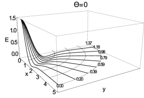
a) b)

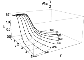
Figure 9: The evaluated interaction energy of the $\Delta\alpha=0$ (in phase), $Q=2+2$ product ansatz Hopfions as a function of the orientation parameters $R$ and $\Phi$ for fixed angles $\Theta=0$ a) and $\Theta=\pi/2$ b).

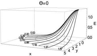
a) b)

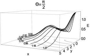
Figure 10: The evaluated interaction energy of the $\Delta\alpha=\pi$ (opposite phase), $Q=2+2$ product ansatz Hopfions as a function of the orientation parameters $R$ and $\Phi$ for fixed angles $\Theta=0$ a) and $\Theta=\pi/2$ b).

Conclusion

We have investigated various interaction channels in the interaction of the axially symmetric ${\cal A}_{1,1}$ and ${\cal A}_{2,1}$ Hopfions. The product ansatz of Hopfions can be obtained via coset projection of the corresponding Skyrme field. This approximation preserves the topological charge in the entire interaction region. In particular, we analysed how the interaction energy depends on the orientation parameters, the separation $R$, the polar angle $\Theta$ and the azimuthal angle $\Phi$.

We have shown that this approach correctly reproduces both the repulsive and attractive interaction channels discussed previously in the limit of the dipole-dipole interactions for ${\cal A}_{1,1}$. Using the product ansatz we also were able to predict interaction pattern for pair of ${\cal A}_{1,1}$ and ${\cal A}_{2,1}$, and two ${\cal A}_{2,1}$ Hopfions. In all cases the interaction has attractive channel for specific orientations and large enough separation distances $R$.

Finally, let us note that the product ansatz can be applied to construct a system of interacting Hopfions of even higher degrees and specific spacial patterns. An approximation to the higher charge linked solitons, whose position curve consists of a few disjoint loops, like for example the configuration in the sector of degree $Q=6$, can be obtained as a multiple product of the projected matrices (9).