Are Markov Models Effective for Storage Reliability Modelling?

Abstract

Continuous Time Markov Chains (CTMC) have been used extensively to model reliability of storage systems. While the exponentially distributed sojourn time of Markov models is widely known to be unrealistic (and it is necessary to consider Weibull-type models for components such as disks), recent work has also highlighted some additional infirmities with the CTMC model, such as the ability to handle repair times. Due to the memoryless property of these models, any failure or repair of one component resets the “clock” to zero with any partial repair or aging in some other subsystem forgotten. It has therefore been argued that simulation is the only accurate technique available for modelling the reliability of a storage system with multiple components (for eg, see [1]).

We show how both the above problematic aspects can be handled when we consider a careful set of approximations in a detailed model of the system. A detailed model has many states, and the transitions between them and the current state captures the “memory” of the various components. We model a non-exponential distribution using a sum of exponential distributions, along with the use of a CTMC solver in a probabilistic model checking tool that has support for reducing large state spaces. Furthermore, it is possible to get results close to what is obtained through simulation and at much lower cost.

1 Introduction

Traditionally, Continuous Time Markov Chains (CTMCs) have been used to model RAID storage system reliability. For small systems, it is possible to construct analytic closed-form expressions for both transient probability of data loss as well as Mean Time To Data Loss (MTTDL). Given some assumptions about the system, such as independent exponential probability distributions for failure and repair, a Markov model can be constructed, resulting often in a nice, closed-form expression. A major problem with this model is that the reliability calculation depends on an extremely simple view of the storage system, especially time independence and the use of reliability models based on exponential probability distributions. Due to the memoryless property of these models, any failure or repair of one component resets the “clock” to zero with any partial repair or aging in some other subsystem forgotten. Hence, simulation has been argued to be the only way to model storage reliability. While individual simulation runs can be fast, simulation for rare events in reliability studies requires many runs to reduce the variance of the results (proportional to $1=\sqrt{p}$, $p$ being the rare event probability) and techniques such as importance sampling have to be used. However, many of its techniques are not easy to use and are still a research topic

In this paper, we show how this problematic aspect of Markov models can be handled when we consider a careful set of approximations in a detailed model of the system. A detailed model has many states, and the transitions between them and the current state captures the “memory” of the various components. We show that with proper approximation of non-exponential distributions with exponential ones, it is possible to accurately model storage reliability using Markov models and get the same results as simulation but much faster. We use a tool named PRISM where each module is written indep and the tool does the interleaving of events, so that much simpler and scalable for programmers/designers (need to write this sentence properly).

2 Problem with Markov Model: Memorylessness

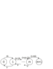
Figure 1: Traditional $m$ disk fault-tolerant Markov model. Taken verbatim from [1].

Several questions have been raised[1] regarding suitability of Markov models as a tool to measure storage reliability. The memorylessness assumption made in these models may affect reliability analysis of a real system in case of multi-disk fault tolerant systems. To make the paper self-contained, we consider the same Markov model for a multi-disk fault tolerant system as in [1] (with Figures 1, 2 taken verbatim) and summarize the insights in that paper below.

With every failure, the system (Figure 1) transitions to a new state but where all the components in the system are reset. In other words, the age of a still functioning available component is reset to 0 (i.e., it becomes new), while any repair of failed components is forgotten. Both cases are problematic. Furthermore, consider a repair that is represented by the transition from state 1 to state 0. Note that the repair of one disk converts all disks into their fresh states. However, only the recently repaired component is new, while all the others have a nonzero age.

Next, consider the system under repair in an intermediate state $i$ with $1<i<m$. On a failure to state $i+1$, any previous rebuild is lost, and only the variable $\mu$ now decides the repair transition back to state $i$. The most recent failure therefore determines the repair transition but it is the earliest failure, whose rebuild is nearest to the finish, that should decide repair transitions.

With the memorylessness assumption, therefore, each transition discards any work completed in a previous state; hence both component wear-out and rebuild progress are not modelled. Such time-dependent aspects are quite difficult to model. Furthermore, according to the analysis in [1], there are differing notions of time: absolute and relative. Absolute time is the time since the start of the system, whereas relative times apply to individual device lifetimes and repair clocks. Since Markov analytic models operate in absolute time, it is not clear how to handle each individual clock. According to Greenan, simulation is therefore the only effective solution to this problem because simulation methods can track relative time and thus can effectively model reliability of a storage system with time-dependent properties.

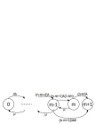
Figure 2: Multi-disk fault tolerant Markov model with latent sector errors. Verbatim from [1]. k and m are the number of data disks and parity disks. h is the BER (bit-error rate) multiplied by the capacity of the device; i.e., the likelihood that a single disk exhibits a bit error if read in its entirety.

Next consider latent sector errors. Any sector error or bit error during rebuild in critical mode can lead to data loss; in a $m$-disk fault tolerant system, the storage system enters critical mode upon the $m$-th disk failure. The transition in the Markov model in Figure 2 from the $m-1$ to the $m+1$ state models data loss due to sector errors in critical mode. However, such a model overestimates the system unreliability. A sector failure only leads to data loss if it occurs in the portion of the failed disk that is critically exposed. For example, in a two-disk fault tolerant system, if the first disk to fail is 90% rebuilt when a second disk fails, only 10% of the disk is critically exposed. This difficulty with Markov models again follows from the memorylessness assumption.

3 Effectiveness of Markov Models

In this paper, we argue that Markov Models are effective in spite of the problems mentioned above; however, this requires using larger state space models. It has been shown that it is possible to approximate many common distributions using a sum of many exponential distributions[2]; it has been computationally difficult in the past however. Given the maturity of CTMC solvers available in tools such as PRISM [3] and its focus on reducing the size of state space, the difficulty is no longer an issue as we show below. To show the effectiveness of this approach, we first show how the reliability of RAID5 can be computed in much faster time than simulation where disk failure is modelled by Weibull distributions.

To handle the incorrect assumption of time independence with respect to rebuild times, note that a a detailed model has many states, and the transitions between them and the current state captures the “memory” of the various components; this enables us to avoid the time independence in large measure. We present our results of modelling rebuild times in Section3.2 and this agrees with simulation results reasonably closely but at a much lower cost in terms of time and effort.

3.1 Case Study 1: Analysis of RAID5 reliability using 3-state Approximation of Weibull Models

Elerath et al. presented a sequential Monte Carlo simulation method, using Weibull failure models, to calculate DDF($t$) for RAID systems where DDF($t$) is the number of double disk failures in time $t$. A DDF occurs when any two disks of a RAID5 group experience operational failure or one disk has a latent defect followed by operational failure from another disk. As PRISM does not support anything other than exponential distributions, we approximate Weibull distributions using phase type distributions (sum of exponentials). We use the same 3 state model (burn-in, normal op, failure due to age) of [5] to approximate each of the Weibull models and find the parameters of the models $\alpha,\sigma,\beta$ using the standard technique of moment matching. Here $\alpha$ is the failure rate during burn-in, $\sigma$ the rate to working state after burn-in and $\beta$ the failure rate after burn-in.

The pdf (probability density function) of the fail state in the 3-state model is:

$$\dfrac{1}{\sigma+\alpha-\beta}[\beta\sigma e^{-\beta t}+(\alpha-\beta)(\sigma+\alpha)e^{-(\sigma+\alpha)t}]$$

The first three moments of this distribution are :

$$\mu_{1} =\frac{\frac{\sigma}{\beta}+\frac{\alpha-\beta}{\alpha+\sigma}}{\alpha-\beta+\sigma}~{}~{}~{}~{}\mu_{2}=\frac{\beta^{2}+\sigma(2\alpha+\sigma)}{\beta^{2}(\alpha+\sigma)^{2}}$$ (1)

$$\mu_{3} =\frac{2\left(1+\frac{-\alpha^{3}+\beta^{3}}{(\alpha+\sigma)^{3}}\right)}{\beta^{3}}.$$ (2)

Solving these three equations, we obtain $\sigma$, $\alpha$ and $\beta$ (eqn. 3).

$$\sigma=\frac{4\mu_{1}^{3}-6\mu_{1}\mu_{2}+\mu_{3}\pm\sqrt{X}}{Y}~{}~{}\alpha=-\frac{2\left(\mu_{1}^{3}-3\mu_{1}\mu_{2}+\mu_{3}\right)}{Y}\\ \beta=\frac{2\mu_{1}^{3}-\mu_{3}\mp\sqrt{X}}{Y}\\ X=-2\mu_{1}^{6}+6\mu_{1}^{4}\mu_{2}-18\mu_{1}^{2}\mu_{2}^{2}+18\mu_{2}^{3}+8\mu_{1}^{3}\mu_{3}-12\mu_{1}\mu_{2}\mu_{3}+\mu_{3}^{2}\\ Y=\mu_{1}^{4}+3\mu_{2}^{2}-2\mu_{1}\mu_{3}\@@generic@caption{}$$ (3)

We use the detailed disk reliability model of Elerath et al.  [4]. Here Time to operational failure (TTOp) (“whole disk failure”) is modelled with a 2-parameter Weibull (shape = 1.12, scale = 461386 hrs) whereas Time to latent defect (TTLd) is modelled as an exponential distribution (equivalent to a Weibull with shape = 1) with scale = 9259 hours. The Time to restore (TTR) or rebuild time has a 3-parameter Weibull (shape = 2, scale = 12 hours and offset 6 hours) while Time to scrub (TTScr) has a 3-parameter Weibull (shape = 3, scale = 168 hours and offset 6 hours). All of the above Weibull failure/repair models have increasing failure rates.

We equate the above moments of the 3-state model with the first three moments of Weibull for each of the three cases: TTOp, TTScr, TTR. For TTOp, the solutions turn out to be $\alpha=1.72E-6$ and either $\sigma=2.49E-6$, $\beta=2.88E-6$ or, equivalently $\sigma=1.16E-6$, $\beta=4.21E-6$

3.1.1 Comparison of Approx. Model with Weibull

To check how well this pdf approximates Weibull distribution, we compare the pdf functions of approximate and Weibull models (Figures 3). The hazard rate for the approximate model becomes constant after some time. This can be understood by looking into the slope of the hazard rate function for the approximate model:

$$\frac{\sigma(\beta-\alpha)e^{-(\sigma+\alpha+\beta)t}}{(\frac{\sigma}{\sigma+\alpha-\beta}e^{-\beta t}+\frac{\alpha-\beta}{\sigma+\alpha-\beta}e^{-(\alpha+\sigma)t})^{2}}$$

Note that the slope function is a non-negative decreasing function for $\beta>\alpha$. Hence after some time slope becomes zero.

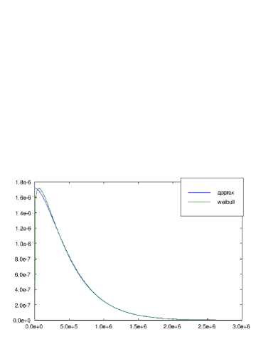
Figure 3: Approximate vs. Weibull pdf; X axis shows time in hrs

To understand the differences better, we look at the differences between the two CDFs (Approximate minus Weibull). The difference is never more than +0.006 or less than -0.003. Therefore, when using the CDFs to compute probabilities of any interval, the results will never be erroneous by more than 0.006 - (-0.003) = 0.009, less than 1%. The differences in the right tails apparently become zero, indicating the approximation to be very good for right tail probabilities.

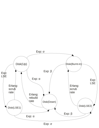
Figure 4: Approximate Disk model based on Gopinath et al.  [6]: one difference is that we consider here a more accurate model that has a transition from Disk(LSE1) state to the Disk(LSE2) state with rate $\sigma$ rather than a transition from Disk(LSE1) to Disk(Burnt-in) state.

For TTR and TTScr, with the same approach, we get a complex number for $\sigma$ and $\beta$ and negative value for $\alpha$ for each of the two solutions respectively. Hence, we use other phase type distributions such as Erlang distributions  [6]. We use a 3-stage Erlang model. For TTScr $\lambda$ = 0.019228232 and for TTR $\lambda$ = 0.180345653. Using these models for each type of failure/repair we build a detailed disk model (Fig.4).

Comparison of PRISM, Monte Carlo Simulation Results:

We compare the reliability of RAID subsystems using PRISM model and Monte Carlo Simulation (Table 1 and Table 2). We try to keep the variance of both PRISM and Monte Carlo Simulation results same so that we can make a fair comparison. Hence, we set the termination epsilon parameter in case of PRISM and the number of experiments parameter in case of Monte Carlo simulation accordingly. Results from Table 1 (under the column with 3-state disk failure model) show that DDF(t) values calculated from PRISM model are similar with those of the Monte Carlo simulation. Due to the front-overloading of our approximate pdf (compared to the actual Weibull pdf), the difference between DDF(t) values calculated using PRISM and Monte Carlo simulation is much higher in the beginning.

Time(yr)	pDDF3(t)	pDDF4(t)	sDDF(t)	sDev3(%)	sDev4(%)
1	7.12	5.59	5.63	26.5	-0.72
2	14.37	12.2	12.23	17.5	-0.21
3	21.67	19.26	19.21	12.8	0.28
4	28.99	26.59	26.43	9.7	0.59
5	36.35	34.06	33.8	7.5	0.75
6	43.73	41.6	41.27	6	0.8
7	51.13	49.17	48.79	4.8	0.77
8	58.54	56.73	56.36	3.9	0.66
9	65.96	64.27	63.93	3.2	0.57
10	73.39	71.78	71.50	2.7	0.38

Table 1: DDF(t) per 1000 RAID groups for 6 disk RAID5: PRISM Model (pDDF_i(t)) vs. Simulation (sDDF(t)). pDDF_i(t)= DDF calculated in PRISM using $i$-state disk failure model. sDev = Deviation of PRISM results from Simulation results; Time taken for Model Checking = 37 sec (using 3-state model) and 4.3 min (using 4-state model) while time for Simulation = 8 min; both PRISM and simulation error are 1%. Number of states using symmetry reduction are 8280 and 33985 with 3-state and 4-state model respectively.

Time(yr)	PRISM DDF(t)	sDDF(t)	sDev(%)
1	2.26	1.92	17.7
2	4.62	3.84	20.3
3	7.03	6.46	8.8
4	9.51	9.32	2
5	12.04	12.16	-1
6	14.63	14.87	-1.6
7	17.27	18.24	-5
8	19.96	21.52	-7.3
9	22.71	24.56	-7.5
10	25.50	28.16	-9.4

Table 2: DDF(t) per 1000000 RAID groups for 8 disk RAID6 : Time taken for Model Checking = 12.6 min while time for Simulation = 26 hr; PRISM error is 1% and Simulation Error is 4%

It can be noted that the higher deviation between the results of PRISM and simulation due to front overloading of the approximate pdf can be reduced by adding more states in the Markov model. We consider a 4-state model to check how well it approximates Weibull. Note that a 4-state Markov model has 5 model parameters. To estimate them using moment matching is hard; we estimate the parameters by matching the hazard rate curve of approximate distribution and Weibull distribution for some time period of interest (0 to 10 yr). Note that the 4-state model does not have an obvious interpretation as the 3-state does. (we need to reword it. We can say we tried free tools avlbl but they were not upto it. Instead of developing another tool, we found it easier to try it by hand).

Table 1 (under the column 4-state disk model) shows the DDF(t) values computed using the 4-state model and how they agree with simulation. Note that in the time period of $t$ = 0 to 10 yr, the deviations are now much less (especially in the initial period).

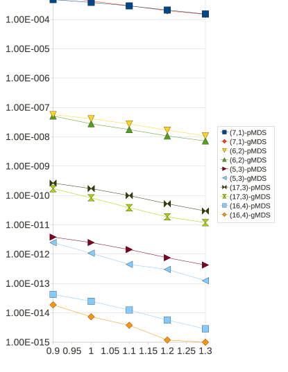
Figure 5: Comparison of PRISM results with Greenan’s simulation results. $X$ and $Y$ axis corresponds to failure shape and the probability of dataloss respectively. $(n,k)$-pMDS and $(n,k)$-gMDS corresponds to the result using PRISM and Greenan’s simulation result respectively. The number of states is less than 1000 for PRISM (we make use of its symmetry reduction capability).

3.2 Case Study 2: Comparison with Greenan’s simulation results for rebuild

For a single disk fault tolerant system, the difficulties of modelling rebuild with Markov models does not arise. In case of multi-disk fault tolerant system (for example RAID6), we compose detailed disk models (Fig.4) to build a disk subsystem model. Hence we consider failure and repair modes of each disk separately rather than considering a system level Markov model like Figures 1 and 2. Moreover, when we approximate Weibull repair and Weibull failure by summation of exponentials (i.e. by adding multiple states and transitions corresponding to a single failure/repair transition) then these states keep information regarding repair progress and age of a component respectively. Hence, our disk subsystem models using detailed disk models reduce the chance of loss of information due to memorylessness property significantly.

To show that Markov models are effective, we use PRISM to model some disk subsystem configurations that use MDS (maximum distance separable) codes from Greenan’s thesis [7], and compare PRISM results with the Greenan’s simulation results from a “high-fidelity simulator” developed only for this purpose. Here, different MDS configurations are analyzed to compute the sensitivity of probability of data loss in 10 years to failure shape parameters. We approximate Weibull failure by a 3-state Markov model and Weibull repair by a 8-stage Erlang model. In both cases we estimate the model parameters by moment matching. For some cases where the model parameters ($\sigma$ and $\beta$) of 3-state Markov model result in a complex number, we estimate the model parameters based on the solution found by moment matching. Our results (Figure 5) show that PRISM results are similar in “order” compared to the simulation results with the advantage that it is very fast (time taken for calculating each data point in Figure 5 is less than 1 sec in PRISM). For some cases with multi-disk fault tolerant systems PRISM results are higher than the simulation results. The possible reasons are

• The front overloading of the approximate pdf (in a 3-state model) w.r.t. Weibull pdf.

• Approximating Weibull distribution using Erlang distribution in case of repair distribution is not good because Weibull repair has a high shape parameter (shape=2).

The success of our technique depends on how well we approximate Weibull distribution using exponentials. For Weibull distribution with high shape parameter the approximation becomes poor as the hazard function for approximate becomes flat for large $t$ whereas for Weibull it is an increasing function (for example, with Weibull shape=2, hazard rate increases linearly with time).

4 Conclusion

In this paper, we have shown that many difficulties due to the memorylessness of Markov models can be handled if more detailed models are considered. A detailed model has many states, and the transitions between them and the current state captures the “memory” of the various components. Hence, we can get good agreement with similar detailed simulated models but at lower cost in time (for example, for rare event failure case such as RAID6, PRISM model is almost 150 times faster than simulation at the same accuracy). We need mature tools such as PRISM to make such detailed Markov models feasible. Simulation may still be the best general method but we also need to consider that validation of the results in a rare event simulation is non-trivial. We believe that the automation that is possible in CTMC solvers as in PRISM (for eg, of interleaving all the failure cases) makes it much simpler to consider detailed models.

5 Bibliography

References

- [1] Kevin M. Greenan, James S. Plank, Jay J. Wylie, “Mean time to meaningless: MTTDL, Markov models, and storage system reliability,” HotStorage (2010).
- [2] Manish Malhotra, Andrew Reibman, “Selecting and Implementing Phase Approximations for Semi-Markov models,” Commun. Statist. -Stochastic Models, 9(4), 1993.
- [3] www.prismmodelchecker.org
- [4] Jon G. Elerath, Michael Pecht, “Enhanced Reliability Modeling of RAID Storage Systems,” DSN 2007
- [5] Qin Xin, Thomas J. E. Schwarz, Ethan L. Miller, “Disk infant mortality in large storage systems,” MASCOTS (2005).
- [6] K. Gopinath, Jon Elerath, Darrell Long, “Reliability Modelling of Disk Subsystems with Probabilistic Model Checking,” UCSC TR 2009
- [7] http://www.kaymgee.com/Kevin_Greenan/Publications_files/kmgreen-thesis.pdf, Sec. 6.4