Event-triggered control under time-varying rates
and channel blackouts

Abstract

This paper studies event-triggered stabilization of linear time-invariant systems over time-varying rate-limited communication channels. We explicitly account for the possibility of channel blackouts, i.e., intervals of time when the communication channel is unavailable for feedback. Assuming prior knowledge of the channel evolution, we study the data capacity, which is the maximum total number of bits that could be communicated over a given time interval, and provide an efficient real-time algorithm to lower bound it for a deterministic time-slotted model of channel evolution. Building on these results, we design an event-triggering strategy that guarantees Zeno-free, exponential stabilization at a desired convergence rate even in the presence of intermittent channel blackouts. The contributions are the notion of channel blackouts, the effective event-triggered control despite their occurrence, and the analysis and quantification of the data capacity for a class of time-varying continuous-time channels. Various simulations illustrate the results.

AND

1 Introduction

Control under communication constraints has key theoretical and practical importance given the increasing ubiquity of networked cyber-physical systems in nearly every aspect of modern life, including transportation, energy, agriculture, and healthcare. This has motivated a vast amount of research to address the challenges posed by communication channels with limited, time-varying, and unreliable bit rates. This paper is a contribution to the growing body of results that employ either information-theoretic or opportunistic triggered control to address the problem of stabilization under constrained resources. Specifically, we seek to combine both approaches to deal with the control of linear time-invariant systems under time-varying channels, including for the possibility of blackouts, i.e., intervals of time during which the channel is completely unavailable for control. Applications where these channel models are useful include communication in contested environments and scheduling shared communication resources.

Literature review: The literature of information-theoretic control under communication constraints focuses on identifying necessary and sufficient conditions on the bit rates that guarantee stabilization under various assumptions on the (often stochastically modeled) communication channels. Comprehensive overviews may be found in (Nair et al., 2007; Franceschetti and Minero, 2014). Early data rate results (Nair and Evans, 2000, 2004; Tatikonda and Mitter, 2004) provided tight necessary and sufficient conditions on the data rate of the encoded feedback for asymptotic stabilization in the discrete-time setting. Since then, the problem has been studied under increasingly complex assumptions on the communication channels, see e.g., (Martins et al., 2006; Minero et al., 2009, 2013). In the continuous-time setting, the problem has been studied under either periodic sampling or aperiodic sampling with known upper and lower bounds on the sampling period. The works (Keyong and Baillieul, 2004, 2007) deal with single-input systems, (Persis, 2005) deals with nonlinear feedforward systems, and (Liberzon, 2014) deals with switched linear systems and characterizes the convergence rate of the finite data-rate stabilization scheme. The recent work (Pearson et al., 2014) explores the stabilization problem under a state-based aperiodic transmission policy, with the inter-transmission intervals being integral multiples of a fixed stepsize. In general, this literature has not explored the potential advantages of tuning the sampling period in the periodic case or if state-based aperiodic sampling can provide any gains in efficiency and performance. On the other hand, the event-triggered approach, see e.g. (Tabuada, 2007; Wang and Lemmon, 2011; Heemels et al., 2012) and references therein, exploits the tolerance to measurement errors to design goal-driven, opportunistic state-based aperiodic sampling. The literature on event-triggered control mainly focuses on guaranteeing control performance while minimizing the number of transmissions but largely ignores quantization, data capacity, and other important aspects of communication. Some of the few exceptions include (Tallapragada and Chopra, 2012; Garcia and Antsaklis, 2013), which utilize static logarithmic quantization and (Lehmann and Lunze, 2010; Li et al., 2012; Sun and Wang, 2014) (see also references therein) which use dynamic quantization. All these works guarantee a positive lower bound on the inter-transmission times, while (Lehmann and Lunze, 2010; Li et al., 2012; Sun and Wang, 2014) also provide a uniform bound on the communication bit rate (i.e., the number of bits per transmission). However, these references do not address the inverse problem of triggering and quantization given a limit on the communication bit rate. Moreover, the channel is assumed to always be available to the control system and hence event-triggered designs typically do not take into account the possibility of channel blackouts. An important exception to this statement is (Anta and Tabuada, 2009), which uses the deadlines generated by a self-triggered controller to perform a kind of instantaneous or short-term scheduling. However, if the communication latency is time-varying either because of a time-varying channel or because of time-varying packet sizes, which is important in finite precision feedback control, it is difficult to guarantee long-term future schedulability and system performance. Our recent work (Tallapragada and Cortés, 2016) combines the information-theoretic and event-triggered control approaches to address the problem of event-triggered stabilization of continuous-time linear time-invariant systems under bounded bit rates. The event-triggered formulation allows us to guarantee, in the absence of channel blackouts, a specified rate of convergence in the presence of non-instantaneous communication and possibly time-varying communication rate. The incorporation of information-theoretic aspects in our design also allows us to analyze sufficient average data rate, something usually absent in the event-triggered literature.

Statement of contributions: We combine information-theoretic and event-triggered control to address the stabilization problem for linear time-invariant systems over time-varying rate-limited communication channels that may be subject to sporadic blackouts. Our starting point is a description of the communication channel through two time-varying channel functions representing, respectively, the minimum instantaneous communication-rate and the maximum packet size that can be successfully transmitted. Our model explicitly accounts for the possibility of channel blackouts, which are intervals of time during which no packet can be successfully transmitted. Our first contribution is the definition of the concept of data capacity, i.e., the maximum number of bits that may be communicated over possibly multiple transmissions during an arbitrary time interval under complete knowledge of the channel evolution. This concept plays a key role in effectively controlling the system despite the occurrence of blackouts. The computation of data capacity for general time-varying channels is challenging. We show that, for the class of piecewise constant channel functions, the computation of data capacity can be formulated as an allocation problem involving the number of bits to be transmitted over each interval where the channel functions are constant. This equivalence sets the basis for our second contribution, which is the design of an algorithm to lower bound in real time the data capacity over an arbitrary time interval. Our third and final contribution is the synthesis of event-triggered control schemes that, using prior knowledge of the channel information, plan the transmissions in order to guarantee the exponential stabilization of the system at a desired convergence rate, even in the presence of intermittent channel blackouts. Our design critically relies on three elements: a performance-trigger function that measures how close the system state is to violating the control objective, a channel-trigger function that keeps track of the number of bits required at any moment to guarantee performance at least for a certain period of time in the future, and the lower bounds on data capacity provided by our real-time algorithm. Our notion of scheduled channel blackouts and stabilization despite their occurrence is a key contribution in the context of event-triggered control, which typically assumes the channel is available for feedback on demand. Various simulations illustrate our results.

Notation: We let $\mathbb{R}$, $\mathbb{R}_{\geq 0}$, ${\mathbb{Z}_{>0}}$, and ${\mathbb{Z}}_{\geq 0}$ denote the set of real, nonnegative real, positive integer, and nonnegative integer numbers, respectively. We let $|S|$ denote the cardinality of the set $S$. We denote by $\|.\|_{2}$ and $\|.\|_{\infty}$ the Euclidean and infinity norm of a vector, respectively, or the corresponding induced norm of a matrix. For a symmetric matrix $A\in\mathbb{R}^{n\times n}$, we let $\lambda_{m}(A)$ and $\lambda_{M}(A)$ denote its smallest and largest eigenvalues, respectively. For any matrix norm $\|.\|$, note that $\|e^{A\tau}\|\leq e^{\|A\|\tau}$. For a number $a\in\mathbb{R}$, we let $\left[a\right]_{+}\triangleq\max\{0,a\}$. For a function $f:\mathbb{R}\mapsto\mathbb{R}^{n}$ and any $t\in\mathbb{R}$, we let $f(t^{-})$ and $f(t^{+})$ denote the limit from the left, $\displaystyle\lim_{s\uparrow t}f(s)$ and the limit from the right, $\displaystyle\lim_{s\downarrow t}f(s)$, respectively.

2 Problem statement

We start with the description of the system dynamics, then describe the model for the communication channel, and finally state the control objective.

2.1 System description

We consider a linear time-invariant control system,

$$\dot{x}(t)=Ax(t)+Bu(t),$$ (1)

where $x\in\mathbb{R}^{n}$ denotes the state of the plant and $u\in\mathbb{R}^{m}$ the control input, while $A\in\mathbb{R}^{n\times n}$ and $B\in\mathbb{R}^{n\times m}$ are the system matrices. Our starting point is the existence of a continuous-time feedback stabilizer of the plant dynamics (1). Formally, we select a control gain matrix $K\in\mathbb{R}^{m\times n}$ such that the matrix $\bar{A}=A+BK$ is Hurwitz. Under this assumption, the continuous-time feedback $u(t)=Kx(t)$ renders the origin of (1) globally exponentially stable.

The plant is equipped with a sensor (the encoder) and an actuator (the decoder) that are not co-located. The sensor can measure the state exactly and the actuator can exert the input to the plant with infinite precision. However, the sensor may transmit state information to the controller at the actuator only at discrete time instants of its choice, using only a finite number of bits. We let $\{t_{k}\}_{k\in{\mathbb{Z}_{>0}}}\subset\mathbb{R}_{\geq 0}$ be the sequence of transmission times at which the sensor transmits an encoded packet of data, $\{r_{k}\}_{k\in{\mathbb{Z}_{>0}}}\subset\mathbb{R}_{\geq 0}$ the sequence of reception times at which the decoder receives a complete packet of data, and $\{\tilde{r}_{k}\}_{k\in{\mathbb{Z}_{>0}}}\subset\mathbb{R}_{\geq 0}$ the sequence of update times at which the decoder updates the controller state. At a transmission time $t_{k}$, the sensor sends $b_{k}$ bits, which encode the plant state. Due to causality, $\tilde{r}_{k}\geq r_{k}\geq t_{k}$, and we denote by

$$\Delta_{k}\triangleq r_{k}-t_{k},\quad\tilde{\Delta}_{k}\triangleq\tilde{r}_{k}-t_{k},$$

the $k^{\text{th}}$ communication time and $k^{\text{th}}$ time-to-update, respectively. The distinction between the reception times and the update times is a generalization with respect to our previous work (Tallapragada and Cortés, 2016) and provides greater flexibility in the presence of time-varying channels, particularly in cases where the channel is unavailable for certain periods of time.

2.2 Communication channel

Our model for the time-varying communication channel is fully determined by the map $R:\mathbb{R}_{\geq 0}\rightarrow\mathbb{R}_{\geq 0}$, where $R_{a}=nR$ is the minimum instantaneous communication-rate at a given time, and the map $\bar{p}:\mathbb{R}_{\geq 0}\rightarrow{\mathbb{Z}}_{\geq 0}$, where $\bar{b}=n\bar{p}$ is the maximum packet size that can be successfully transmitted at a given time. More specifically, we assume the $k^{\text{th}}$ communication time and the $k^{\text{th}}$ time-to-update satisfy

$$\tilde{\Delta}_{k}\geq\Delta_{k}\geq 0,$$ (2a)

$$\Delta_{k}\leq\Delta(t_{k},p_{k})\triangleq\frac{p_{k}}{R(t_{k})}=\frac{b_{k}}{R_{a}(t_{k})},$$ (2b)

where the first condition is that of causal communication and the second is an upper bound on the communication time. Note that the actual instantaneous communication rate at $t_{k}$ is $b_{k}/\Delta_{k}$ and we can rewrite (2b) as

$$\frac{b_{k}}{\Delta_{k}}=\frac{np_{k}}{\Delta_{k}}\geq\frac{np_{k}}{\Delta(t_{k},p_{k})}=R_{a}(t),$$

to realize that $R_{a}(t)$ is a lower bound on the number of bits communicated per unit time of all the bits transmitted at time $t$. Thus, for example, if $R_{a}(t)=\infty$, then the packet sent at $t$ is received instantaneously. The packet size $b_{k}=np_{k}$ that can be successfully transmitted starting at $t_{k}$ is upper bounded as

$$p_{k}\leq\bar{p}(t_{k}),\quad p_{k}\in{\mathbb{Z}}_{\geq 0}$$ (3a)

for all $$k\in{\mathbb{Z}}_{\geq 0} \bar{p}=\bar{b}=0 t\mapsto R(t) t\mapsto\bar{p}(t)$$. We refer to an interval of time during which as a (channel) blackout. In this paper, we assume that the encoder knows the functions and a priori or sufficiently in advance, which we make clear in the sequel.

Since the channel has bounded data capacity and in order to maintain synchronization between the encoder and the decoder, we require that the encoder does not transmit a packet before a previous packet is received by the decoder and the controller updated, i.e.,

$$t_{k+1}\geq\tilde{r}_{k},$$ (3b)

for all $k\in{\mathbb{Z}}_{\geq 0}$. We say the channel is busy at time $t$ if $t\in[t_{k},r_{k})$, for some $k\in{\mathbb{Z}_{>0}}$. Finally, we refer to the sequences of transmission times $\{t_{k}\}\subset\mathbb{R}_{\geq 0}$, packet sizes $\{b_{k}\}\subset{\mathbb{Z}}_{\geq 0}$, and update times $\{\tilde{r}_{k}\}\subset\mathbb{R}_{\geq 0}$ as feasible if (2) and (3) are satisfied for every $k\in{\mathbb{Z}_{>0}}$.

2.3 Encoding and decoding

We use dynamic quantization for finite-bit transmissions from the encoder to the decoder. In dynamic quantization, there are two distinct phases: the zoom-out stage, e.g., (Liberzon, 2003), during which no control is applied while the quantization domain is expanded until it captures the system state at time $r_{0}=t_{0}\in\mathbb{R}_{\geq 0}$; and the zoom-in stage, during which the encoded feedback is used to asymptotically stabilize the system. We focus exclusively on the latter, i.e., for $t\geq t_{0}$. We assume both the encoder and the decoder have perfect knowledge of the plant system matrices, have synchronized clocks, and synchronously update their states at update times $\{\tilde{r}_{k}\}_{k\in{\mathbb{Z}_{>0}}}$. For simplicity, we assume that at transmission $t_{k}$ the sensor (encoder) encodes each dimension of the plant state using $p_{k}$ bits so that the total number of bits transmitted is $b_{k}=np_{k}$.

The state of the encoder/decoder is composed of the controller state $\hat{x}\in\mathbb{R}^{n}$ and an upper bound $d_{e}\in\mathbb{R}_{\geq 0}$ on $\|x_{e}\|_{\infty}$, where $x_{e}\triangleq x-\hat{x}$ is the encoding error. Thus, the actual input to the plant is given by $u(t)=K\hat{x}(t)$. During inter-update times, the state of the dynamic controller evolves as

$$\dot{\hat{x}}(t)=A\hat{x}(t)+Bu(t)=\bar{A}\hat{x}(t),\quad t\in[\tilde{r}_{k},\tilde{r}_{k+1}).$$ (4a)

Let the encoding and decoding functions at the $$k^{\text{th}} q_{E,k}:\mathbb{R}^{n}\times\mathbb{R}^{n}\mapsto G_{k} q_{D,k}:G_{k}\times\mathbb{R}^{n}\mapsto\mathbb{R}^{n} G_{k} 2^{b_{k}} t_{k} z_{E,k}\triangleq q_{E,k}(x(t_{k}),\hat{x}(t_{k}^{-})) \hat{x}(t_{k}^{-}) t_{k} z_{D,k}\triangleq q_{D,k}(z_{E,k},\hat{x}(t_{k}^{-})) [r_{k},\tilde{r}_{k}] \tilde{r}_{k} \hat{x}$$ iteration be represented by and , respectively, where is a finite set of symbols. At , the encoder encodes the plant state as , where is the controller state just prior to the encoding time , and sends it to the controller. The decoder can decode this signal as at any time during . At the update time , the sensor and the controller also update using the jump map,

$$\hat{x}(\tilde{r}_{k}) =e^{\bar{A}\tilde{\Delta}_{k}}\hat{x}(t_{k}^{-})+e^{A\tilde{\Delta}_{k}}(z_{D,k}-\hat{x}(t_{k}^{-}))$$

$$\triangleq q_{k}(x(t_{k}),\hat{x}(t_{k}^{-})),$$ (4b)

where $q_{k}:\mathbb{R}^{n}\times\mathbb{R}^{n}\mapsto\mathbb{R}^{n}$ represents the quantization that occurs as a result of the finite-bit coding. We allow the quantization domain, the number of bits and the resulting quantizer, $q_{k}$, for each transmission $k\in{\mathbb{Z}_{>0}}$ to be variable. The evolution of the plant state $x$ and the encoding error $x_{e}$ on the time interval $[\tilde{r}_{k},\tilde{r}_{k+1})$ can be written as

$$\dot{x}(t) =\bar{A}x(t)-BKx_{e}(t),$$ (5a)

$$\dot{x}_{e}(t) =Ax_{e}(t).$$ (5b)

While the encoder knows the encoding error $x_{e}$ precisely, the decoder can only compute a bound $d_{e}(t)$ on $\|x_{e}(t)\|_{\infty}$ as follows

$$d_{e}(t) \triangleq\|e^{A(t-t_{k})}\|_{\infty}\delta_{k},\ t\in[\tilde{r}_{k},\tilde{r}_{k+1}),\ k\in{\mathbb{Z}}_{\geq 0}$$ (6a)

$$\delta_{k+1} =\frac{1}{2^{p_{k+1}}}d_{e}(t_{k+1}).$$ (6b)

One can design a pair of algorithms for the encoder and the decoder to implement (4) in a manner that they maintain consistent $\hat{x}(t)$ and $d_{e}(t)$ signals for $t\geq t_{0}$ (see (Tallapragada and Cortés, 2016) for example). For the sake of brevity, we do not present these algorithms here and it suffices to say that $\|x_{e}(t)\|_{\infty}\leq d_{e}(t)$ for all $t\geq t_{0}$ if $\|x_{e}(t_{0})\|_{\infty}\leq d_{e}(t_{0})$.

2.4 Control objective

We measure the performance of the closed-loop system through a Lyapunov function as follows. Given an arbitrary symmetric positive definite matrix $Q\in\mathbb{R}^{n\times n}$, let $P$ be the unique symmetric positive definite matrix that satisfies the Lyapunov equation

$$P\bar{A}+\bar{A}^{T}P=-Q.$$ (7)

Define $x\mapsto V(x)=x^{T}Px$ and let

$$V_{d}(t)=V_{d}(t_{0})e^{-\beta(t-t_{0})},$$ (8)

with $\beta>0$, be the desired control performance. We assume that

$$W \triangleq\frac{\lambda_{m}(Q)}{\lambda_{M}(P)}-a\beta>0,$$ (9)

with $a>1$ an arbitrary constant. Assumption (9) is sufficient to guarantee a convergence rate faster than $\beta$ for the dynamics (1) under the continuous-time and unquantized feedback $u(t)=Kx(t)$.

Given the system and the communication channel model above, our objective is to design an event-triggered communication and control strategy that ensures the exponential stability of the origin. Formally, we seek to synthesize an event-triggered control strategy that recursively determines the sequences of transmission times $\{t_{k}\}_{k\in{\mathbb{Z}_{>0}}}$ and update times $\{\tilde{r}_{k}\}_{k\in{\mathbb{Z}_{>0}}}$, along with a coding scheme for messages and a rule to determine the number of bits $\{b_{k}\}_{k\in{\mathbb{Z}_{>0}}}$ to be transmitted, so that

$$V(x(t))\leq V_{d}(t),$$

holds for all $t\geq t_{0}$. This objective is especially challenging given the time-varying nature of the communication channel and the possibility of intermittent blackouts.

3 Performance- and channel-trigger functions

In order to achieve the control objective of Section 2.4 with opportunistic transmissions, we need a performance-trigger function that tells us how close the system state is to violating the convergence requirement. Bounded precision quantization further requires us to keep track (through a channel-trigger function) of the number of bits required at any moment to guarantee performance at least for a certain period of time. Threshold crossings of these two functions form the primary basis of our event-triggering mechanism. Further, in order to take care of communication delays, the triggering mechanism instead uses guaranteed upper bounds on the performance and channel-trigger functions up to the maximum possible communication delay for the current channel state. In this section, we describe each of these components, thus laying the groundwork to deal with time-varying communication channels and blackouts.

3.1 Performance-trigger function

We define the performance-trigger function as the ratio of the quadratic Lyapunov function $V$ and the desired performance $V_{d}$,

$$h_{\operatorname{pf}}(t)\triangleq\frac{V(x(t))}{V_{d}(t)}.$$ (10)

Note that the control objective is to maintain $h_{\operatorname{pf}}(t)\leq 1$ at all times. This is why, in general, it is of interest to characterize the open-loop evolution of the performance-trigger function. The next result provides an upper bound on the value of $h_{\operatorname{pf}}$ in the future as a function of the information available now.

Lemma 3.1.

(Upper bound on open-loop evolution of performance-trigger function (Tallapragada and Cortés, 2016)). Given $t_{k}\in\mathbb{R}_{>0}$ such that $h_{\operatorname{pf}}(t_{k})\leq 1$, then

$$h_{\operatorname{pf}}(\tau+t_{k})\leq\bar{h}_{\operatorname{pf}}(\tau,h_{\operatorname{pf}}(t_{k}),\epsilon(t_{k})),$$

for $\tau\geq 0$, where

$$\epsilon(t)\triangleq\frac{d_{e}(t)}{c\sqrt{V_{d}(t)}},\quad\bar{h}_{\operatorname{pf}}(\tau,h_{0},\epsilon_{0})\triangleq\frac{f_{1}(\tau,h_{0},\epsilon_{0})}{f_{2}(\tau)},$$ (11)

$$f_{1}(\tau,h_{0},\epsilon_{0})\triangleq h_{0}+\frac{W\epsilon_{0}}{w+\mu}(e^{(w+\mu)\tau}-1),\quad f_{2}(\tau)\triangleq e^{w\tau},$$

$$c\triangleq\frac{W\sqrt{\lambda_{m}(P)}}{2\sqrt{n}\|PBK\|_{2}},\;w\triangleq\frac{\lambda_{m}(Q)}{\lambda_{M}(P)}-\beta>0,\;\mu\triangleq\|A\|_{2}+\frac{\beta}{2}.$$

This result motivates the definition of the function

$$\Gamma_{1}(h_{0},\epsilon_{0})\triangleq\min\{\tau\geq 0:\bar{h}_{\operatorname{pf}}(\tau,h_{0},\epsilon_{0})=1,\ \frac{\mathrm{d}\bar{h}_{\operatorname{pf}}}{\mathrm{d}\tau}\geq 0\},$$

as a lower bound on the time it takes $h_{\operatorname{pf}}$ to evolve to $1$ starting from $h_{\operatorname{pf}}(t_{k})=h_{0}$ with $\epsilon(t_{k})=\epsilon_{0}$. The following result captures some useful properties of this function.

Lemma 3.2.

(Properties of the function $\Gamma_{1}$ (Tallapragada and Cortés, 2016)). The following holds true,

1. $\Gamma_{1}(1,1)>0$.

2. If $h_{1}\geq h_{0}$ and $\epsilon_{1}\geq\epsilon_{0}$, then $\Gamma_{1}(h_{0},\epsilon_{0})\geq\Gamma_{1}(h_{1},\epsilon_{1})$. In particular, if $h_{0}\in[0,1]$, then $\Gamma_{1}(h_{0},\epsilon_{0})\geq\Gamma_{1}(1,\epsilon_{0})$.

3. For $T>0$, if $h_{0}\in[0,1]$ and

   $$\epsilon_{0}\leq\rho_{T}(h_{0})\triangleq\frac{(w+\mu)(1-h_{0})}{W(e^{(w+\mu)T}-1)}+1,$$ (12)

   then $\Gamma_{1}(h_{0},\epsilon_{0})\geq\min\{\Gamma_{1}(1,1),T\}$.

4. For $T>0$ and $h_{0}\in[0,1]$,

   $$\Gamma_{1}(h_{0},\epsilon_{0})\geq T\Longleftrightarrow\bar{h}_{\operatorname{pf}}(T,h_{0},\epsilon_{0})\leq 1.$$

   The statement with strict inequalities is also true.

3.2 Channel-trigger function

We define the channel-trigger function

$$h_{\operatorname{ch}}(t)\triangleq\frac{\epsilon(t)}{\rho_{T}(h_{\operatorname{pf}}(t))},$$ (13)

where $T>0$ is a fixed design parameter. The channel-trigger function $h_{\operatorname{ch}}$ depends on the bound on the encoding error $d_{e}$ through $\epsilon$. Note that the channel-trigger function $h_{\operatorname{ch}}$ through its dependence on $d_{e}$, which evolves as (6), also jumps at the update times $\tilde{r}_{k}$. Lemma 3.2(iii) implies that for any time $s_{0}\geq t_{0}$, if $h_{\operatorname{ch}}(s_{0})\leq 1$, then $h_{\operatorname{pf}}(t)\leq 1$ for at least $t\in[s_{0},s_{0}+\min\{T,\Gamma_{1}(1,1)\})$ even without any transmissions or receptions. Thus, assuming that the communication delays are smaller than $\min\{T,\Gamma_{1}(1,1)\}$, a transmission strategy ( $\{t_{k}\}_{k\in{\mathbb{Z}_{>0}}}$ and $\{b_{k}\}_{k\in{\mathbb{Z}_{>0}}}$ such that $b_{k}=np_{k}$) is to ensure that, for each $k$, $h_{\operatorname{ch}}(\tilde{r}_{k})\leq 1$ so that $\Gamma_{1}(h_{\operatorname{pf}}(\tilde{r}_{k}),\epsilon(\tilde{r}_{k}))\geq\min\{T,\Gamma_{1}(1,1)\}$. Thus, we now require an upper bound on the open-loop evolution of $h_{\operatorname{ch}}$, which is provided in the following result. Its proof follows from the definitions of $\epsilon$ and $\rho_{T}$ in (11) and (12), respectively, and the evolution of $d_{e}$ described in (6).

Lemma 3.3.

(Upper bound on the channel-trigger function at the update times $\tilde{r}_{k}$). If $t_{k}\in\mathbb{R}_{>0}$ is such that $h_{\operatorname{pf}}(t_{k})\in[0,1]$, then

$$h_{\operatorname{ch}}(\tilde{r}_{k})\leq\bar{h}_{\operatorname{ch}}(\tilde{r}_{k}-t_{k},h_{\operatorname{pf}}(t_{k}),\epsilon(t_{k}),p_{k}),$$ (14)

where $b_{k}=np_{k}$ bits are transmitted at $t_{k}$ and

$$\bar{h}_{\operatorname{ch}}(\tau,h_{0},\epsilon_{0},p)\triangleq\frac{\|e^{A\tau}\|_{\infty}e^{\frac{\beta}{2}\tau}\epsilon_{0}}{\rho_{T}(\bar{h}_{\operatorname{pf}}(\tau,h_{0},\epsilon_{0}))}\cdot\frac{1}{2^{p}}.$$ (15)

Note that for $t,t+\tau\in[\tilde{r}_{k},t_{k+1})$, for any $k\in{\mathbb{Z}}_{\geq 0}$, we have $h_{\operatorname{ch}}(t+\tau)\leq\bar{h}_{\operatorname{ch}}(\tau,h_{\operatorname{pf}}(t),\epsilon(t),0)$.

Now, analogous to $\Gamma_{1}$, we define

$$\Gamma_{2}(b_{0},\epsilon_{0},p) \triangleq\min\{\tau\geq 0:\bar{h}_{\operatorname{ch}}(\tau,b_{0},\epsilon_{0},p)=1\},$$ (16)

which essentially is an upper bound on the communication delay $\tilde{r}_{k}-t_{k}$, for which we can still guarantee $h_{\operatorname{ch}}(\tilde{r}_{k})\leq 1$. Given the interpretation of $\Gamma_{2}$, one of the conditions in our event-triggering rule would be to check if $\Gamma_{2}$ is less than a maximum communication delay. The next result provides a way to check this in real time.

Lemma 3.4.

(Algebraic condition to check value of $\Gamma_{2}$ (Tallapragada and Cortés, 2016)). Let $T^{\circ}>0$. For any $h_{0}\in[0,1]$ and $\epsilon_{0}\in[0,\rho_{T}(h_{0})]$, $\Gamma_{2}(h_{0},\epsilon_{0},p)>T^{\circ}$ if and only if $\bar{h}_{\operatorname{ch}}(T^{\circ},h_{0},\epsilon_{0},p)<1$. Further, the statement with equalities is also true.

The following result provides a lower bound for $\Gamma_{2}$ uniform in its first two arguments. This bound will be useful in our event-triggered design later.

Lemma 3.5.

(Lower bound on $\Gamma_{2}$). If $\epsilon_{0}\in[0,\rho_{T}(h_{0})]$ then $\Gamma_{2}(h_{0},\epsilon_{0},p)\geq T^{*}(p)$ with

$$T^{*}(p) \triangleq\min\{\tau\geq 0:g(\tau,p)=1\},$$

$$g(\tau,p) \triangleq\frac{\|e^{A\tau}\|_{\infty}e^{\frac{\beta}{2}\tau}}{2^{p}}\cdot\frac{e^{(w+\mu)T}-1}{e^{(w+\mu)T}-e^{(w+\mu)\tau}}.$$

From (10) and (12), we have

$$\rho_{T}(\bar{h}_{\operatorname{pf}}(\tau,h_{0},\epsilon_{0}))$$

$$=\frac{(w+\mu)(1-e^{-w\tau}(h_{0}+\frac{W\epsilon_{0}}{w+\mu}(e^{(w+\mu)\tau}-1)))}{W(e^{(w+\mu)T}-1)}+1$$

$$=\rho_{T}(e^{-w\tau}h_{0})-\frac{e^{(w+\mu)\tau}-1}{e^{(w+\mu)T}-1}e^{-w\tau}\epsilon_{0}$$

$$\geq\rho_{T}(e^{-w\tau}h_{0})\frac{e^{(w+\mu)T}-e^{(w+\mu)\tau}}{e^{(w+\mu)T}-1},$$

where the inequality follows from the assumption that $\epsilon_{0}\leq h_{0}$. Now, substituting this lower bound in (15) and noting the fact that $\rho_{T}(e^{-w\tau}h_{0})\geq\rho_{T}(h_{0})$ gives

$$\bar{h}_{\operatorname{ch}}(\tau,h_{0},\epsilon_{0},p)\leq g(\tau,p).$$

The claim now follows from the definition (16). ∎

4 Characterization of the data capacity

Our study of data capacity here is motivated by the need of the encoder to know how much data can be transmitted successfully before a channel blackout.

4.1 Data capacity

We denote the number of bits (data) communicated (the data transmitted by the encoder and completely received by the decoder) during the time interval $[\tau_{1},\tau_{2}]$ under the feasible sequences $\{t_{k}\}$, $\{p_{k}\}$, and $\{\tilde{\Delta}_{k}\}$ (that satisfy (2) and (3)) as

$$D(\tau_{1},\tau_{2},\{t_{k}\},\{\tilde{\Delta}_{k}\},\{p_{k}\})\triangleq n\sum_{k=\underline{k}_{\tau_{1}}}^{\overline{k}_{\tau_{2}}}p_{k},$$

where $\underline{k}_{\tau_{1}}=\min\{k:t_{k}\geq\tau_{1}\}$ and $\overline{k}_{\tau_{2}}=\max\{k:t_{k}+\tilde{\Delta}_{k}\leq\tau_{2}\}$. Notice that we count only the bits that are transmitted and also received (communicated) during $[\tau_{1},\tau_{2}]$. We define the data capacity during the time interval $[\tau_{1},\tau_{2}]$ as the maximum data that can be communicated during the time interval under all possible communication delays, i.e.,

$$\mathcal{D}(\tau_{1},\tau_{2})\triangleq\max_{\begin{subarray}{c}\{t_{k}\},\{p_{k}\}\\ \text{s.t. \eqref{eqn:feas-seq} holds}\\ \forall\Delta_{k}\leq\Delta(t_{k},p_{k})\end{subarray}}D(\tau_{1},\tau_{2},\{t_{k}\},\{\Delta_{k}\},\{p_{k}\}).$$

Notice that to maximize the data communicated, it must be that $\tilde{r}_{k}=r_{k}$ ($\tilde{\Delta}_{k}=\Delta_{k}$) for all $k\in{\mathbb{Z}_{>0}}$. This explains the fact that only the sequences $\{t_{k}\}$ and $\{p_{k}\}$ are the optimization variables. Next, notice that maximization under all possible communication delays ($\Delta_{k}\leq\Delta(t_{k},p_{k})$) is the same as maximization under maximum communication delays ($\Delta_{k}=\Delta(t_{k},p_{k})$). Thus, the definition of the data capacity reduces to

$$\mathcal{D}(\tau_{1},\tau_{2})\triangleq\max_{\begin{subarray}{c}\{t_{k}\},\{p_{k}\}\\ \text{s.t. \eqref{eqn:feas-seq} holds}\end{subarray}}D(\tau_{1},\tau_{2},\{t_{k}\},\{\Delta(t_{k},p_{k})\},\{p_{k}\}).$$ (17)

Note that a greedy approach does not necessarily maximize the communicated data. In general, the precise computation of $\mathcal{D}(\tau_{1},\tau_{2})$ involves solving an integer program with non-convex feasibility constraints. Given the difficulty of solving this problem, we seek a class of channel functions $R$ and $\bar{b}$ that are meaningful and yet simple enough to efficiently compute a lower bound for the data capacity. To this end, we make the following observation.

Lemma 4.1.

(Data capacity under constant communication rate). Suppose $\forall t\in[\tau_{1},\tau_{2}]$ (i) $R(t)=R\geq 0$ and (ii) $\bar{p}(t)\geq 1$ (no blackouts). Then, $\mathcal{D}(\tau_{1},\tau_{2})=n\lfloor R(\tau_{2}-\tau_{1})\rfloor$.

The proof of Lemma 4.1 follows directly by noting that an optimal solution can be constructed by choosing $p_{k}=1$ and $t_{k+1}=\tilde{r}_{k}=r_{k}$ for all $k\in{\mathbb{Z}}_{\geq 0}$. Motivated by this result, we assume in the sequel that the channel function $R$ is piecewise constant so that the problem of finding a reasonable lower bound on $\mathcal{D}(\tau_{1},\tau_{2})$ is tractable while also ensuring that the overall problem is meaningful. Note that any given $R$ can be approximated to an arbitrary degree of accuracy by a piecewise constant function. In addition, according to (2b), $R$ is a lower bound on the instantaneous communication rate and it is quite reasonable to assume it is piecewise constant. Also, note that $\bar{p}$ takes integer values and hence by its nature is always piecewise constant. Specifically, we assume that

$$R(t) =R_{j},\quad\forall t\in(\theta_{j},\theta_{j+1}]$$ (18a)

$$\bar{p}(t) =\bar{\pi}_{j},\quad\forall t\in(\theta_{j},\theta_{j+1}]$$ (18b)

where $\{\theta_{j}\}_{j=0}^{\infty}$ is a strictly increasing sequence of time instants and $\bar{\pi}_{j}\in{\mathbb{Z}}_{\geq 0}$ for each $j$. We also denote $T_{j}\triangleq\theta_{j+1}-\theta_{j}$ as the length of the $j^{\text{th}}$ time slot $I_{j}\triangleq(\theta_{j},\theta_{j+1}]$. Again note that identical $\{\theta_{j}\}$ sequences for $R$ and $\bar{p}$ is not a restriction because one can always refine the sequence $\{\theta_{j}\}$. In order to concisely express the constraints in the optimization problem (17) we assume, without loss of generality, that $\tau_{1}=\theta_{j_{0}}$ and $\tau_{2}=\theta_{j_{f}}$, for some $j_{0},j_{f}\in{\mathbb{Z}}_{\geq 0}$. Finally, we choose left-open intervals in our model (18) since it provides a slight technical advantage in lowering the gap between the optimal and our sub-optimal solutions.

4.2 Formulation as an allocation problem

Here we show that, for piecewise constant channel functions, we can think of the computation of $\mathcal{D}(\theta_{j_{0}},\theta_{j_{f}})$ as an allocation problem: that of allocating the number of bits $\{n\phi_{j}\}$, with $\phi_{j}\in{\mathbb{Z}}_{\geq 0}$, to be transmitted in the time slots $\{I_{j}\}$ for $j\in\mathcal{N}_{j_{0}}^{j_{f}}\triangleq\{j_{0},\ldots,j_{f}-1\}$. For convenience, we let $\phi_{j_{0}}^{j_{f}}\triangleq(\phi_{j_{0}},\ldots,\phi_{j_{f}-1})$. Given $\phi_{j_{0}}^{j_{f}}$, the sequences $\{t_{k}\}$ and $\{p_{k}\}$ are determined so that transmissions start at the earliest possible time in $I_{j}$ and the channel is not idle until all the allocated bits $\phi_{j}$ are received, i.e., $t_{k+1}=\tilde{r}_{k}=r_{k}=\Delta(t_{k},p_{k})$ during $I_{j}$ and $\{p_{k}\}$ during $I_{j}$ is any sequence that respects the channel upper bound $\bar{\pi}_{j}$ and adds up to $\phi_{j}$. Given this correspondance, our forthcoming discussion focuses on expressing the constraints in the optimization problem in terms of the $\phi$ variables. In the sequel, a standing constraint is that $\phi_{j}\in{\mathbb{Z}}_{\geq 0}$ for each $j$, unless we mention otherwise.

Maximum bits that may be transmitted: First, we present the constraint that describes the maximum bound on the number of bits that may be transmitted in each slot $I_{j}$. Note that according to Lemma 4.1, in the time slot $I_{j}$, $n\lfloor R_{j}T_{j}\rfloor$ bits could be transmitted and received within $\lfloor R_{j}T_{j}\rfloor/R_{j}\leq T_{j}$ units of time. In addition, $n\bar{\pi}_{j}$ more bits could be transmitted during the closed interval $[\ \lfloor R_{j}T_{j}\rfloor,\theta_{j+1}]$, though these bits are received only in subsequent time slots. Thus, we have for each $j\in\mathcal{N}_{j_{0}}^{j_{f}}$

$$n\phi_{j}\leq\begin{cases}nR_{j}T_{j}+n\bar{\pi}_{j},\quad&\text{if }\bar{\pi}_{j}>0\\ 0,\quad&\text{if }\bar{\pi}_{j}=0\end{cases}$$ (19)

where in the first case we have used the fact that $\phi_{j}\in{\mathbb{Z}}_{\geq 0}$ to avoid the use of the floor function.

Reduced channel availability in a time slot due to prior transmissions: As noted above, if $\phi_{j}>\lfloor R_{j}T_{j}\rfloor$, then these bits take up some of the time in $I_{j+1}$ and possibly even subsequent slots. Thus, effectively the time available in $I_{j+1}$ and consequently the upper bound on $\phi_{j+1}$ is reduced. Moreover, in general, the number of bits transmitted in $I_{j}$ has an effect on the number that could be transmitted in all subsequent intervals either directly or indirectly. Thus, for each $j_{1},j\in\mathcal{N}_{j_{0}}^{j_{f}}$, we introduce

$$\bar{T}_{j_{1},j}(\phi_{j_{0}}^{j_{f}}) \triangleq\Big{(}T_{j}-\sum_{i=j_{1}}^{j-1}\big{(}\frac{\phi_{i}}{R_{i}}-T_{i}\big{)}\Big{)}$$

$$=\theta_{j+1}-\theta_{j_{1}}-\sum_{i=j_{1}}^{j-1}\frac{\phi_{i}}{R_{i}}.$$ (20)

As we shall see in the following lemma, these functions determine the available time in slot $I_{j}$ given $\phi_{j_{0}}^{j_{f}}$.

Lemma 4.2.

(Available time in slot $I_{j}$). Let $\bar{T}_{j}(\phi_{j_{0}}^{j_{f}})$ be the time available in the slot $I_{j}$ given the allocation $\phi_{j_{0}}^{j_{f}}$. Then,

$$\bar{T}_{j}(\phi_{j_{0}}^{j_{f}})=\Big{[}\min_{j_{1}\in\mathcal{N}_{j_{0}}^{j_{f}}}\{\bar{T}_{j_{1},j}(\phi_{j_{0}}^{j_{f}}),T_{j}\}\Big{]}_{+}.$$

Observe that for any $j_{1},j\in\mathcal{N}_{j_{0}}^{j_{f}}$, $\theta_{j+1}-\theta_{j_{1}}$ is the total time in the slots $j_{1}$ to $j$, while $\sum_{i=j_{1}}^{j-1}\frac{\phi_{i}}{R_{i}}$ is the total time taken by the bits transmitted in slots $j_{1}$ to $j-1$. Thus, $\left[\bar{T}_{j_{1},j}(\phi_{j_{0}}^{j_{f}})\right]_{+}$ is an upper bound on the time available for transmission in the slot $I_{j}$. Now, let

$$j_{2}=\max\{i\in{\mathbb{Z}}_{\geq 0}\operatorname{\cap}[j_{0},j-1]:\bar{T}_{i}(\phi_{j_{0}}^{j_{f}})=T_{i}\}$$

Then clearly, $\{\phi_{i}\}_{i=j_{2}}^{j-1}$ is sufficient to determine $\bar{T}_{j}(\phi_{j_{0}}^{j_{f}})$. Next, for the allocation $\phi_{j_{0}}^{j_{f}}$, the bits transmitted during the time slots $I_{i}$ for $i\in\{j_{2},j-1\}$ are received by $\theta_{j_{2}}+\sum_{j=j_{2}}^{j-1}\tfrac{\phi_{j}}{R_{j}}$ and thus in deed $\bar{T}_{j}(\phi_{j_{0}}^{j_{f}})=\left[\min\{\bar{T}_{j_{2},j}(\phi_{j_{0}}^{j_{f}}),T_{j}\}\right]_{+}$. Finally, for each $j_{1}\in{\mathbb{Z}}_{\geq 0}\operatorname{\cap}[j_{0},j_{2}-1]$, $\bar{T}_{j_{1},j}(\phi_{j_{0}}^{j_{f}})\geq\bar{T}_{j_{2},j}(\phi_{j_{0}}^{j_{f}})$, which proves the result. ∎

As a consequence of Lemma 4.2, for each $j\in\mathcal{N}_{j_{0}}^{j_{f}}$ and $j_{1}\in{\mathbb{Z}}_{\geq 0}\operatorname{\cap}[j_{0},j-1]$, consider the constraints

$$n\phi_{j}\leq\begin{cases}nR_{j}\bar{T}_{j_{1},j}(\phi_{j_{0}}^{j_{f}})+n\bar{\pi}_{j},&\text{if }\bar{T}_{j_{1},j}(\phi_{j_{0}}^{j_{f}})>0\\ 0&\text{otherwise}\end{cases}$$ (21a)

which we obtain using the same reasoning as in (19) with $$T_{j} \bar{T}_{j_{1},j}(\phi_{j_{0}}^{j_{f}}) \bar{T}_{j_{1},j}(\phi_{j_{0}}^{j_{f}})\geq T_{j} \bar{T}_{j_{1},j}(\phi_{j_{0}}^{j_{f}})\in(0,T_{j}) I_{j} \bar{T}_{j_{1},j}(\phi_{j_{0}}^{j_{f}})\leq 0 j_{1}\in{\mathbb{Z}}_{\geq 0}\operatorname{\cap}[j_{0},j-1] I_{j} \bar{T}_{j}(\phi_{j_{0}}^{j_{f}})=0 I_{j}$$ replaced by . Note that if , then the constraint (21a) is weaker than (19) and hence inactive. For , the constraint reflects the reduced available time in the time slot and if , for some , then it corresponds to the case when the channel is busy for the whole of the time slot (). Thus (21a) accurately reflects the effect of possibly reduced available time during the slot due to prior transmissions.

Counting only the bits transmitted and received during $[\theta_{j_{0}},\theta_{j_{f}}]$: Finally, since in the computation of $\mathcal{D}(\theta_{j_{0}},\theta_{j_{f}})$, we are interested in the maximum number of bits that can be communicated (transmitted and received) during the time interval, we also require that any bits transmitted during the slot $I_{j}$ are received before $\theta_{j_{f}}$, i.e.,

$$\frac{\phi_{j}}{R_{j}}\leq\begin{cases}\bar{T}_{j}(\phi_{j_{0}}^{j_{f}})+\theta_{j_{f}}-\theta_{j+1},&\text{if }\bar{T}_{j}(\phi_{j_{0}}^{j_{f}})>0\\ 0,&\text{otherwise}.\end{cases}$$

Using the definition of $\bar{T}_{j}(\phi_{j_{0}}^{j_{f}})$, this can be rewritten giving the following constraints for each $j\in\mathcal{N}_{j_{0}}^{j_{f}}$ and $j_{1}\in{\mathbb{Z}}_{\geq 0}\operatorname{\cap}[j_{0},j]$

$$\frac{\phi_{j}}{R_{j}}\leq\begin{cases}\bar{T}_{j_{1},j}(\phi_{j_{0}}^{j_{f}})+\theta_{j_{f}}-\theta_{j+1},&\text{if }\bar{T}_{j_{1},j}(\phi_{j_{0}}^{j_{f}})>0\\ 0,&\text{otherwise}.\end{cases}$$ (21b)

Then, the data capacity is given as

$$\mathcal{D}(\theta_{j_{0}},\theta_{j_{f}})=\max_{\begin{subarray}{c}\phi_{j}\in{\mathbb{Z}}_{\geq 0},\forall j\in\mathcal{N}_{j_{0}}^{j_{f}}\\ \text{s.t. \eqref{eqn:max-bit-bound-Ij}, \eqref{eqn:case-constraints} hold}\end{subarray}}\;n\sum_{j=j_{0}}^{j_{f}-1}\phi_{j}.$$ (22)

Ignoring the fact that this is an integer program, the constraints (21) still make the problem combinatorial.

4.3 Efficient approximation of data capacity

The following result is the basis for the construction of a sub-optimal and efficient solution to the problem (22).

Lemma 4.3.

(Bound on “channel variation”). If there exists $J\in{\mathbb{Z}}_{\geq 0}$ such that

$$\frac{\bar{\pi}_{j}}{R_{j}}<\sum_{i=j+1}^{i=j+1+J}T_{i},\quad\forall j\in\mathcal{N}_{j_{0}}^{j_{f}},$$ (23)

then, for any $j\in\mathcal{N}_{j_{0}}^{j_{f}}$, any bits transmitted in time slot $I_{j}$ would be received strictly before the end of the slot $I_{j+1+J}$.

The term $\bar{\pi}_{j}/R_{j}$ is the time it takes a packet of size up to $n\bar{\pi}_{j}$ bits transmitted during $I_{j}$ to reach the decoder. Thus, the claim follows by noting that any bits transmitted during $I_{j}$ would be received before $t=~{}\theta_{j+1}+(\bar{\pi}_{j}/R_{j})$. ∎

Lemma 4.3 relates the three sequences of parameters, $\{R_{j}\}$, $\{\bar{\pi}_{j}\}$ and $\{T_{j}\}$, that define the channel state at any given time. The result may be interpreted as the imposition of a bound on how often there is a change in the channel state as measured by the time slot lengths $T_{j}$. The parameter $J$ may be interpreted as a uniform upper bound on the number of consecutive time slots that may be fully occupied due to a prior transmission.

4.3.1 Guaranteed channel availability in each time slot

The case of $J=0$ is of special interest and will be addressed next. This case is interesting because the constraints (21) reduce to a simpler form, as presented in the following result, and using which we can compute a good sub-optimal solution subsequently.

Lemma 4.4.

(Data capacity in the case of $J=0$). Suppose the channel is such that $J=0$ for all $j\in\mathcal{N}_{j_{0}}^{j_{f}}$. Then, the constraints (21a) reduce to

$$n\phi_{j}+nR_{j}\sum_{i=j_{1}}^{j-1}\frac{\phi_{i}}{R_{i}}\leq nR_{j}(\theta_{j+1}-\theta_{j_{1}})+n\bar{\pi}_{j},$$ (24a)

for each $$j\in\mathcal{N}_{j_{0}}^{j_{f}} j_{1}\in{\mathbb{Z}}_{\geq 0}\operatorname{\cap}[j_{0},j-1]$$ and while the constraints (21b) reduce to

$$\sum_{i=j_{1}}^{j_{f}-1}\frac{\phi_{i}}{R_{i}}\leq\theta_{j_{f}}-\theta_{j_{1}},$$ (24b)

for each $$j_{1}\in{\mathbb{Z}}_{\geq 0}\operatorname{\cap}[j_{0},j_{f}-1]$$.

The data capacity is

$$\mathcal{D}(\theta_{j_{0}},\theta_{j_{f}})=\max_{\begin{subarray}{c}\phi_{j}\in{\mathbb{Z}}_{\geq 0},\forall j\in\mathcal{N}_{j_{0}}^{j_{f}}\\ \text{s.t. \eqref{eqn:max-bit-bound-Ij}, \eqref{eqn:case-constraints-J0} hold}\end{subarray}}\;n\sum_{j=j_{0}}^{j_{f}-1}\phi_{j}.$$ (25)

Indeed, if $J=0$ then for each $j$ and $j_{1}\in\mathcal{N}_{j_{0}}^{j_{f}}$, $\bar{T}_{j_{1},j}(\phi_{j_{0}}^{j_{f}})>0$ and hence $\bar{T}_{j}>0$ also. Thus, the constraints (21a) reduce to $n\phi_{j}\leq nR_{j}\bar{T}_{j_{1},j}(\phi_{j_{0}}^{j_{f}})+n\bar{\pi}_{j}$, which after using (4.2) give us (24a). Note that Lemma 4.3, with $J=0$, guarantees that the constraints (21b) are satisfied for all $j\in\{j_{0},\ldots,j_{f}-2\}$, while for $j_{f}-1$  (21b) reduce to

$$\frac{\phi_{j_{f}-1}}{R_{j_{f}-1}}\leq\bar{T}_{j_{1},j}(\phi_{j_{0}}^{j_{f}}),$$

which by expanding and rearranging the terms, we get the constraints (24b). Data capacity (25) follows from (22) and the equivalence of (21) and (24). ∎

Note that for $J=0$ all the constraints, (19) and (24) are linear, though $\phi_{j}$ are still restricted to be integers. This brings us to the next result.

Proposition 4.5.

(A sub-optimal solution and quantification of sub-optimality in the case of $J=0$). Suppose the channel is such that $J=0$ for all $j\in\mathcal{J}=\{j_{0},\ldots,j_{f}\}$. Let $\mathcal{D}_{s}(\theta_{j_{0}},\theta_{j_{f}})\triangleq n\sum_{j=j_{0}}^{j_{f}-1}\phi^{N}_{j}$ where

$$\phi^{N}\triangleq\lfloor\phi^{r}\rfloor\triangleq(\lfloor\phi^{r}_{j_{0}}\rfloor,\ldots,\lfloor\phi^{r}_{j_{f}-1}\rfloor),$$ (26)

$$\phi^{r}=\!\!\operatorname*{argmax}_{\begin{subarray}{c}\phi_{j}\in\mathbb{R}_{\geq 0},\ \forall j\in\mathcal{N}_{j_{0}}^{j_{f}}\\ \text{s.t. \eqref{eqn:max-bit-bound-Ij}, \eqref{eqn:case-constraints-J0} hold}\end{subarray}}\;\sum_{j=j_{0}}^{j_{f}-1}\phi_{j}.$$

Then $\phi^{N}$ is a sub-optimal solution to (25), i.e. $\mathcal{D}_{s}(\theta_{j_{0}},\theta_{j_{f}})\leq\mathcal{D}(\theta_{j_{0}},\theta_{j_{f}})$ and

$$\mathcal{D}(\theta_{j_{0}},\theta_{j_{f}}) -\mathcal{D}_{s}(\theta_{j_{0}},\theta_{j_{f}})$$

$$\leq n|\{j\in{\mathbb{Z}}_{\geq 0}\operatorname{\cap}[j_{0},j_{f-1}]:\bar{\pi}_{j}>0\}|.$$

Clearly, $\phi^{N}$ satisfies the constraints (19) and (24) since $\phi^{r}$ does and for each $j$, $\phi^{N}_{j}\leq\phi^{r}_{j}$ and $\phi^{N}\in{\mathbb{Z}}_{\geq 0}$. Thus, $\phi^{N}$ is a sub-optimal solution to (25). The sub-optimality bound follows from the fact that for any $a\in\mathbb{R}$, $(a-\lfloor a\rfloor)\in[0,1)$. ∎

4.3.2 No guaranteed channel availability

If $J>0$, we forgo optimality in favor of an easily computable lower bound of the data capacity. With a slight abuse of notation, we let

$$\phi^{N}_{j}=\lfloor R_{j}(\theta_{j+1}-\theta_{j})\rfloor,\quad j\in{\mathbb{Z}}_{\geq 0},$$

which is the number of bits that can be communicated (transmitted and received) during the time slot $I_{j}=[\theta_{j},\theta_{j+1})$. Hence, $\{\phi_{j}^{N}\}_{j\in{\mathbb{Z}}_{\geq 0}}$ is a feasible solution and, again with an abuse of notation, we denote

$$\mathcal{D}_{s}(\theta_{j_{0}},\theta_{j_{f}})\triangleq n\sum_{j=j_{0}}^{j_{f}-1}\phi^{N}_{j},$$

which is a sub-optimal lower bound of the data capacity.

4.4 Computing data capacity in real time

As mentioned earlier, we want the encoder to compute a lower bound for the data capacity up to the end of the next blackout period. However, the computation of $\mathcal{D}_{s}(\tau_{1},\tau_{2})$ in the case of $J=0$ involves solving a linear program and hence may not be suitable for real-time computation. Thus, given $\mathcal{D}(\theta_{j_{0}},\theta_{j_{f}})$ (or $\mathcal{D}_{s}(\theta_{j_{0}},\theta_{j_{f}})$), we propose a simpler procedure to compute a lower bound on $\mathcal{D}(t,\theta_{j_{f}})$ (or $\mathcal{D}_{s}(t,\theta_{j_{f}})$) for any $t\in[\theta_{j_{0}},\theta_{j_{0}+1})$. We present the procedure in the following result.

Proposition 4.6.

(Real-time computation of data capacity). Let $\phi^{*}$ (or $\phi^{N}$) be any optimizing solution to $\mathcal{D}(\theta_{j_{0}},\theta_{j_{f}})$ (or $\mathcal{D}_{s}(\theta_{j_{0}},\theta_{j_{f}})$). Let

$$\hat{\mathcal{D}}(t,\theta_{j_{f}}) \triangleq\left[n\left\lfloor\phi^{*}_{j_{0}}-R_{j_{0}}(t-\theta_{j_{0}})\right\rfloor\right]_{+}+n\sum_{j=j_{0}+1}^{j_{f}-1}\phi^{*}_{j}$$ (27)

$$\hat{\mathcal{D}}_{s}(t,\theta_{j_{f}}) \triangleq\left[n\left\lfloor\phi^{N}_{j_{0}}-R_{j_{0}}(t-\theta_{j_{0}})\right\rfloor\right]_{+}+n\sum_{j=j_{0}+1}^{j_{f}-1}\phi^{N}_{j},$$ (28)

for any $t\in[\theta_{j_{0}},\theta_{j_{0}+1})$. Then, $0\leq\mathcal{D}(t,\theta_{j_{f}})-\hat{\mathcal{D}}(t,\theta_{j_{f}})\leq n$ and $0\leq\mathcal{D}_{s}(t,\theta_{j_{f}})-\hat{\mathcal{D}}_{s}(t,\theta_{j_{f}})\leq n$.

Here we prove only the statements about $\mathcal{D}(t,\theta_{j_{f}})$ as the proof of the statements for $\mathcal{D}_{s}(t,\theta_{j_{f}})$ are exactly analogous to those of $\mathcal{D}(t,\theta_{j_{f}})$. First of all notice that for any $\tau_{1}<\tau_{2}<\tau_{3}$

$$\mathcal{D}(\tau_{1},\tau_{3})\geq\mathcal{D}(\tau_{1},\tau_{2})+\mathcal{D}(\tau_{2},\tau_{3}).$$ (29)

Now, let $\mathcal{T}_{0}=\theta_{j_{0}}+\frac{\phi^{*}_{j_{0}}}{R_{j_{0}}}$. Clearly, from the optimality of $\mathcal{D}(\theta_{j_{0}},\theta_{j_{f}})$, it follows that

$$\mathcal{D}(\theta_{j_{0}},\mathcal{T}_{0})=n\phi^{*}_{j_{0}},\quad\mathcal{D}(\mathcal{T}_{0},\theta_{j_{f}})=n\sum_{j=j_{0}+1}^{j_{f}-1}\phi^{*}_{j}.$$ (30)

Thus, for the special choice of $\mathcal{T}_{0}$, we have the stronger relation $\mathcal{D}(\theta_{j_{0}},\theta_{j_{f}})=\mathcal{D}(\theta_{j_{0}},\mathcal{T}_{0})+\mathcal{D}(\mathcal{T}_{0},\theta_{j_{f}})$. Now, using (29) twice we get

$$\mathcal{D}(\theta_{j_{0}},\theta_{j_{f}}) \geq\mathcal{D}(\theta_{j_{0}},t)+\mathcal{D}(t,\theta_{j_{f}})$$

$$\geq\mathcal{D}(\theta_{j_{0}},t)+\mathcal{D}(t,\mathcal{T}_{0})+\mathcal{D}(\mathcal{T}_{0},\theta_{j_{f}}),$$

which implies

$$\mathcal{D}(\theta_{j_{0}},\theta_{j_{f}})-\mathcal{D}(\theta_{j_{0}},t)\geq\mathcal{D}(t,\theta_{j_{f}})\geq\mathcal{D}(t,\mathcal{T}_{0})+\mathcal{D}(\mathcal{T}_{0},\theta_{j_{f}}).$$

Notice that $\mathcal{D}(t,\mathcal{T}_{0})+\mathcal{D}(\mathcal{T}_{0},\theta_{j_{f}})=\hat{\mathcal{D}}(t,\theta_{j_{f}})$. Now, we compute the difference between the upper and lower bounds on $\mathcal{D}(t,\theta_{j_{f}})$

$$\mathcal{D}(\theta_{j_{0}},\theta_{j_{f}})-\mathcal{D}(\theta_{j_{0}},t)-\hat{\mathcal{D}}(t,\theta_{j_{f}})$$

$$=\mathcal{D}(\theta_{j_{0}},\mathcal{T}_{0})+\mathcal{D}(\mathcal{T}_{0},\theta_{j_{f}})-\mathcal{D}(\theta_{j_{0}},t)-\hat{\mathcal{D}}(t,\theta_{j_{f}})$$

$$=n\left[R_{j_{0}}(\mathcal{T}_{0}-\theta_{j_{0}})-\lfloor R_{j_{0}}(t-\theta_{j_{0}})\rfloor-\lfloor R_{j_{0}}(\mathcal{T}_{0}-t)\rfloor\right]$$

$$=n\left[-\lfloor R_{j_{0}}(t-\theta_{j_{0}})\rfloor-\lfloor-R_{j_{0}}(t-\theta_{j_{0}})\rfloor\right]\leq n,$$

where, in arriving at the second last relation, we have used $\lfloor R_{j_{0}}(\mathcal{T}_{0}-t)\rfloor=\lfloor R_{j_{0}}(\mathcal{T}_{0}-\theta_{j_{0}})-R_{j_{0}}(t-\theta_{j_{0}})\rfloor$ and the fact that $R_{j_{0}}(\mathcal{T}_{0}-\theta_{j_{0}})=\phi^{*}_{j_{0}}$ is an integer. The statement now follows. ∎

The significance of Proposition 4.6 is that it provides a method to reuse a previously computed solution to find a tight sub-optimal solution to the data capacity problem in real-time. The implication is that, if one has the computational resources, then one may solve the full optimization problem $\mathcal{D}(\theta_{j_{1}},\theta_{j_{2}})$ for $j_{1},j_{2}\in{\mathbb{Z}}_{\geq 0}$ and use the above result to find a tight sub-optimal solution $\hat{\mathcal{D}}(t,\theta_{j_{2}})$ for any $t\in[\theta_{j_{1}},\theta_{j_{1}+1}]$.

5 Event-triggered stabilization

In this section, we address the problem of event-triggered control under a time-varying channel. Section 5.1 address the case with no channel blackouts. Section 5.2 builds on this design and analysis to deal with the presence of channel blackouts.

5.1 Control in the absence of channel blackouts

In the case of no channel blackouts, the encoder may choose to transmit at any time and, in addition, we assume the channel rate $R$ is sufficiently high at all times (the exact technical assumption is specified later) so that there is no need to resort to the computation of data capacity. For this reason, we are able to consider arbitrary (i.e., not necessarily piecewise constant) functions $t\mapsto R(t)$. Note that, by its discrete nature, the function $t\mapsto\bar{p}(t)$ is always piecewise constant. For any $p\in{\mathbb{Z}}_{\geq 0}$, let

$$T_{M}(p)=\sigma\min\{\Gamma_{1}(1,1),T,T^{*}(p)\},$$ (31)

where $\sigma\in(0,1)$ is a design parameter, $T$ is the parameter chosen in (12) and $T^{*}$ is as defined in Lemma 3.5. As we show in the sequel, if $T_{M}(p)$ is an upper bound on the communication delay when $b=np$ bits are transmitted, then it is sufficient to design an event-triggering rule that guarantees the control objective is met.

In the presence of communication delays, we need to make sure (i) that the control objective is not violated between a transmission and the resulting control update and (ii) that at the control update times, the encoding error is sufficiently small to ensure future performance. To this end, we define

$$\mathcal{L}_{1}(t) \triangleq\bar{h}_{\operatorname{pf}}\left(T_{M}(\bar{p}(t)),h_{\operatorname{pf}}(t),\epsilon(t)\right),$$ (32a)

$$\mathcal{L}_{2}(t) \triangleq\bar{h}_{\operatorname{ch}}\left(T_{M}(\bar{p}(t)),h_{\operatorname{pf}}(t),\epsilon(t),\bar{p}(t))\right),$$ (32b)

to take care of each of these requirements. If up to $\bar{b}=n\bar{p}$ bits are transmitted at time $t$, then $\mathcal{L}_{1}(t)$ provides an upper bound on the performance-trigger function $h_{\operatorname{pf}}$ at the reception time which would be less than $t+T_{M}(\bar{p}(t))$, while $\mathcal{L}_{2}(t)$ provides an upper bound on the channel-trigger function $h_{\operatorname{ch}}$ if the control is updated as soon as the packet is received.

Theorem 5.1.

(Event-triggered control in the absence of blackouts). Suppose $t\mapsto\bar{p}(t)$ is piecewise constant, as in (18b), with a uniform lower bound $1$ (i.e., no blackouts) and a uniform upper bound $p^{\max}$. Assume that

$$R(t)\geq\frac{p}{T_{M}(p)},\ \forall p\in\{1,\dots,{\bar{p}(t)}\},\ \forall t.$$ (33)

Consider the system (1) under the feedback law $u=K\hat{x}$, with $t\mapsto\hat{x}(t)$ evolving according to (4) and the sequence $\{t_{k}\}_{k\in{\mathbb{Z}}_{\geq 0}}$ determined recursively by

$$t_{k+1}=\min\{t\geq\tilde{r}_{k}:\ \mathcal{L}_{1}(t)\geq 1\ \lor\ \mathcal{L}_{1}(t^{+})\geq 1\ \lor\$$

$$\mathcal{L}_{2}(t)\geq 1\ \lor\ \mathcal{L}_{2}(t^{+})\geq 1\}.$$ (34)

Let $\{r_{k}\}_{k\in{\mathbb{Z}}_{\geq 0}}$ and $\{\tilde{r}_{k}\}_{k\in{\mathbb{Z}}_{\geq 0}}$ be given as $\tilde{r}_{0}=r_{0}=t_{0}$ and $\tilde{r}_{k}=r_{k}\leq t_{k}+\Delta_{k}$ for $k\in{\mathbb{Z}_{>0}}$. Assume the encoding scheme is such that (6) is satisfied for all $t\geq t_{0}$. Further assume that $\mathcal{L}_{1}(t_{0})\leq 1$, $\mathcal{L}_{2}(t_{0})\leq 1$ and that (9) holds. Let $\underline{p_{k}}$ be

$$\underline{p_{k}}\!\triangleq\!\min\{p\in{\mathbb{Z}_{>0}}:\bar{h}_{\operatorname{ch}}\left(\frac{p}{R(t_{k})},h_{\operatorname{pf}}(t_{k}),\epsilon(t_{k}),p\right)\leq 1\}.$$ (35)

Then, the following hold:

1. $\underline{p_{1}}\leq\bar{p}(t_{1})$. Further for each $k\in{\mathbb{Z}_{>0}}$, if $p_{k}\in{\mathbb{Z}_{>0}}\operatorname{\cap}[\underline{p_{k}},\bar{p}(t_{k})]$, then $\underline{p_{k+1}}\leq\bar{p}(t_{k+1})$.

2. the inter-transmission times $\{t_{k+1}-t_{k}\}_{k\in{\mathbb{Z}_{>0}}}$ and inter-update times $\{\tilde{r}_{k+1}-\tilde{r}_{k}\}_{k\in{\mathbb{Z}_{>0}}}$ have a uniform positive lower bound,

3. the origin is exponentially stable for the closed-loop system, with $V(x(t))\leq V_{d}(t_{0})e^{-\beta(t-t_{0})}$ for $t\geq t_{0}$.

We start by establishing two claims that we later invoke to establish the result.

Claim (a): First, we show that for any $t\geq t_{0}$, if $h_{\operatorname{pf}}(t)\leq 1$ and $h_{\operatorname{ch}}(t)\leq 1$ then $\mathcal{L}_{1}(s)<1$ and $\mathcal{L}_{2}(s)<1$, with $s=t$ and $s=t^{+}$. Indeed, if $h_{\operatorname{pf}}(t)\leq 1$ and $h_{\operatorname{ch}}(t)\leq 1$, then Lemma 3.2 says $\Gamma_{1}(h_{\operatorname{pf}}(t),\epsilon(t))\geq\min\{\Gamma_{1}(1,1),T\}$. Then, from (31), (32a) and from Lemma 3.2(iv), we see that the claim is true for $\mathcal{L}_{1}$. Again, the conditions $h_{\operatorname{pf}}(t)\leq 1$ and $h_{\operatorname{ch}}(t)\leq 1$ along with Lemma 3.5 guarantee that for any $p\in{\mathbb{Z}}_{\geq 0}$, $\Gamma_{2}(h_{\operatorname{pf}}(t),\epsilon(t),p)\geq T^{*}(p)$. Thus, (31), (32b) and Lemma 3.4 imply that the claim is true for $\mathcal{L}_{2}$.

Claim (b): Next, we claim that for any $k\in{\mathbb{Z}}_{\geq 0}$, if $h_{\operatorname{pf}}(\tilde{r}_{k})\leq 1$ and $h_{\operatorname{ch}}(\tilde{r}_{k})\leq 1$, then $\mathcal{L}_{i}(t_{k+1})\leq 1$, for $i\in\{1,2\}$. If the signal $\bar{p}$ is constant during $[\tilde{r}_{k},t_{k+1}]$, the claim immediately follows from Claim (a) and (5.1). Now, let us suppose there exists $\theta\in[\tilde{r}_{k},t_{k+1})$ at which time $\bar{p}$ is discontinuous, i.e., $\theta\in\{\theta_{j}\}_{j\in{\mathbb{Z}_{>0}}}$ as defined by (18b). Then, from (5.1), it is clear that, for $i\in\{1,2\}$, $\mathcal{L}_{i}(\theta)<1$ and $\mathcal{L}_{i}(\theta^{+})<1$. This implies that there exists an interval $\mathcal{I}_{\theta}=[\theta,\theta+\epsilon)$ such that $\mathcal{L}_{i}(s)<1$ for each $s\in\mathcal{I}_{\theta}$ and $i\in\{1,2\}$. Then, by continuity of $\mathcal{L}_{i}$ on each interval $(\theta_{j},\theta_{j+1}]$ and by invoking induction over the discontinuity times of $\bar{p}$, we can conclude that the claim is true.

Now, we show that (i) holds. The facts $\mathcal{L}_{1}(t_{0})\leq 1$ and $\mathcal{L}_{2}(t_{0})\leq 1$ together with the arguments used above ensure that $\mathcal{L}_{1}(t_{1})\leq 1$ and $\mathcal{L}_{2}(t_{1})\leq 1$. Then, (35) ensures that $\underline{p_{1}}\leq\bar{p}(t_{1})$. Now, for each $k\in{\mathbb{Z}_{>0}}$, if $\mathcal{L}_{1}(t_{k})\leq 1$ and $\mathcal{L}_{2}(t_{k})\leq 1$ and $p_{k}\in{\mathbb{Z}_{>0}}\operatorname{\cap}[\underline{p_{k}},\bar{p}(t_{k})]$ then

$$\tilde{r}_{k}-t_{k}=r_{k}-t_{k}\leq\frac{p_{k}}{R(t_{k})}\leq\frac{\bar{p}(t_{k})}{R(t_{k})}\leq T_{M}(\bar{p}(t)),$$ (36)

where the last inequality follows from (33). As a result of (36), we see that $h_{\operatorname{pf}}(\tilde{r}_{k})\leq 1$ and $h_{\operatorname{ch}}(\tilde{r}_{k})\leq 1$. Then, invoking Claim (b), we see that $\mathcal{L}_{2}(t_{k+1})\leq 1$, from which it follows that $\underline{p_{k+1}}\leq\bar{p}(t_{k+1})$, which proves (i).

Now, we prove (ii) - the main idea here is that for each $k\in{\mathbb{Z}}_{\geq 0}$, either $\tilde{r}_{k}-t_{k}$ or $t_{k+1}-\tilde{r}_{k}$ is sufficiently large to guarantee (ii). To show this, we pick a $\sigma_{1}\in(0,1)$ and partition the set ${\mathbb{Z}}_{\geq 0}$ into two subsets $G$ and $L$ defined as follows

$$G =\{k\in{\mathbb{Z}}_{\geq 0}:\tilde{r}_{k}-t_{k}>\sigma_{1}T_{M}(p_{k})\},$$

$$L =\{k\in{\mathbb{Z}}_{\geq 0}:\tilde{r}_{k}-t_{k}\leq\sigma_{1}T_{M}(p_{k})\}.$$

Then, it is clear that $\{t_{k+1}-t_{k}\}_{k\in G}$ and $\{\tilde{r}_{k+1}-\tilde{r}_{k}\}_{k\in G}$ are uniformly lower bounded by $\sigma_{1}T_{M}(1)$. Thus, all that remains is to handle the set $L$. Recall that the assumptions and the design are such that, for each $k\in{\mathbb{Z}}_{\geq 0}$, we guarantee $h_{\operatorname{pf}}(\tilde{r}_{k})\leq 1$ and $h_{\operatorname{ch}}(\tilde{r}_{k})\leq 1$ for $\tilde{r}_{k}\leq t_{k}+T_{M}(p_{k})$. As a result, and due to the fact that $\{p_{k}\}$ is upper bounded by $p^{\max}$, there exist $h_{\operatorname{pf}}^{0},h_{\operatorname{ch}}^{0}\in(0,1)$ such that $h_{\operatorname{pf}}(\tilde{r}_{k})\leq h_{\operatorname{pf}}^{0}$ and $h_{\operatorname{ch}}(\tilde{r}_{k})\leq h_{\operatorname{ch}}^{0}$ for all $k\in L$. Thus, from Claim (a) and (5.1), it is clear that for any $k\in L$, $t_{k+1}-\tilde{r}_{k}\geq T_{L}$, where $T_{L}$ is a lower bound on the time it takes $h_{\operatorname{pf}}$ to evolve from $h_{\operatorname{pf}}^{0}$ to $1$ and on the time it takes $h_{\operatorname{ch}}$ to evolve from $h_{\operatorname{ch}}^{0}$ to $1$. Finally, by the fact that both $h_{\operatorname{pf}}^{0}$ and $h_{\operatorname{ch}}^{0}$ are strictly less than $1$, it follows that $T_{L}>0$, which proves (ii).

Regarding (iii), we have already seen that for any $k\in{\mathbb{Z}}_{\geq 0}$, $h_{\operatorname{pf}}(t)\leq 1$ for all $t\in[t_{k},\tilde{r}_{k}]$. Further, (5.1) also ensures that $h_{\operatorname{pf}}(t)\leq 1$ for all $t\in[\tilde{r}_{k},t_{k+1}]$. Therefore $h_{\operatorname{pf}}(t)\leq 1$ ($V(x(t)\leq V_{d}(t)$) for all $t\geq t_{0}$, which completes the proof. ∎

The interpretation of the three claims of the result is as follows. Claim (i) essentially states that if the number of bits transmitted in the past is according to the given recommendation, then in the future, the sufficient number of bits $\underline{b_{k}}=n\underline{p_{k}}$ to guarantee continued performance will respect the time-varying channel constraints. Claim (ii) is sufficient to guarantee non-Zeno behavior and claim (iii) states that indeed the control objective is met.

Remark 5.2.

(Requirements on the knowledge of channel information). Note that in the scenario with no channel blackouts, the encoder needs to know the channel information given by $R$ and $\bar{p}$ only over a time horizon of length $\delta_{t}$. Further, if a uniform lower bound on $t\mapsto\bar{p}(t)$ greater than or equal to $1$ is known, then it is sufficient for the encoder to know only the channel information at the current time and use this bound to schedule the transmissions (however, this might result in more frequent transmissions with smaller packet sizes). $\bullet$

5.2 Control in the presence of channel blackouts

Here, we address the scenario of channel blackouts building on our developments in Section 5.1. The main difficulty comes from the fact that in the presence of blackouts, the channel might be completely unavailable. Thus, the event-triggering condition not only needs to be based on the functions $\mathcal{L}_{1}$ and $\mathcal{L}_{2}$ in (32), but also on the available data capacity up to the next blackout.

Throughout the section, we assume both $R$ and $\bar{p}$ are piecewise constant functions, as in (18) and, without loss of generality, that time slots with $\bar{p}=0$ are not consecutive. We let $B_{k}\triangleq(\theta_{j_{k}},\theta_{j_{k}+1}]$ denote the $k^{\text{th}}$ blackout slot, with $k\in{\mathbb{Z}_{>0}}$. Also, for any $t\geq t_{0}$, we let

$$\tau_{l}(t) \triangleq\min\{s\geq t:\bar{p}(s)=0\},$$

$$\tau_{u}(t) \triangleq\min\{s\geq\tau_{l}(t):\bar{p}(s)>0\},$$

give, respectively, the beginning and the end times of the next channel blackout slot from the current time $t$. When there is no confusion, we simply use $\tau_{l}$ and $\tau_{u}$, dropping the argument $t$. Hence, for $t\in[t_{0},\theta_{j_{1}})$, we have $\tau_{l}(t)=\theta_{j_{1}}$ and $\tau_{u}(t)=\theta_{j_{1}+1}$. Similarly, for any $k\in{\mathbb{Z}_{>0}}$ and $t\in(\theta_{j_{k}},\theta_{j_{k+1}}]$, we have $\tau_{l}(t)=\theta_{j_{k+1}}$ and $\tau_{u}(t)=\theta_{j_{k+1}+1}$. At time $t$, the length of the next channel blackout slot, $T_{b}(t)\triangleq\tau_{u}(t)-\tau_{l}(t)$, determines a sufficient upper bound on the encoding error $d_{e}(\tau_{l})$, or equivalently $\epsilon(\tau_{l})$, for non-violation of the control objective during the blackout or immediately subsequent to it. We quantify this upper bound in the following result.

Lemma 5.3.

(Upper bound on required $\epsilon$ before blackout). For $t\in[t_{0},\infty)$, suppose

$$\epsilon(\tau_{l}(t))\leq\epsilon_{r}(t)\triangleq\min\left\{\frac{(e^{wT_{b}(t)}-1)(w+\mu)}{W(e^{(w+\mu)T_{b}(t)}-1)},\frac{1}{e^{\bar{\mu}T_{b}(t)}}\right\},$$ (37)

where $\bar{\mu}\triangleq\|A\|_{\infty}+\frac{\beta}{2}$. If $h_{\operatorname{pf}}(\tau_{l}(t))\leq 1$, then $h_{\operatorname{pf}}(s)\leq 1$ for all $s\in[\tau_{l}(t),\tau_{u}(t)]$ and $h_{\operatorname{ch}}(\tau_{u}(t))\leq 1$ (in particular $\epsilon(\tau_{u}(t))\leq 1$).

From Lemma 3.2, we know $\Gamma_{1}(h_{\operatorname{pf}}(\tau_{l}),\epsilon(\tau_{l}))\geq\Gamma_{1}(1,\epsilon_{r}(t))$. So, we need to show that $\Gamma_{1}(1,\epsilon_{r}(t))\geq T_{b}(t)$ or, as per Lemma 3.2(iv), that $\bar{h}_{\operatorname{pf}}(T_{b}(t),1,\epsilon_{r}(t))\leq 1$. Direct computation shows that this is indeed the case, which implies $h_{\operatorname{pf}}(s)\leq 1$ for all $s\in[\tau_{l},\tau_{u}]$ by the definition of $\Gamma_{1}$. The second claim follows from

$$h_{\operatorname{ch}}(\tau_{u}) \leq\bar{h}_{\operatorname{ch}}(T_{b}(t),1,\epsilon_{r}(t),0)$$

$$=\|e^{AT_{b}(t)}\|_{\infty}e^{\frac{\beta}{2}T_{b}(t)}\epsilon_{r}(t)\leq e^{\bar{\mu}T_{b}(t)}\epsilon_{r}(t)\leq 1.\quad\square$$

The ability to ensure that $\epsilon(\tau_{l})$ is sufficiently small is determined by the data capacity $\mathcal{D}(t,\tau_{l})$. To have a real-time implementation, we make use of the sub-optimal lower bound $\hat{\mathcal{D}}_{s}(t,\tau_{l})$ instead. However, notice that maximizing the data throughput and satisfying the primary control goal of exponential convergence at a desired rate may not be compatible in general - if maximizing data throughput is the only goal, then certain transmissions might be delayed and this might lead to the violation of the primary control objective. Conversely, if the control objective is the only goal, this might lead to an inefficient use of the channel that could be detrimental later. Thus, to still be able to use the intuition and the building blocks from Section 5.1, we need to impose a time-varying artificial bound on the allowed packet size in place of $\bar{p}(t)$ that prevents the system from affecting the data capacity until the next blackout. To this end, we store in the variable $\mathcal{P}_{j}$ the value of $\phi^{N}_{j}$, where $\phi^{N}$ is as defined in Section 4.3 for $\mathcal{D}_{s}(\theta_{j},\tau_{l}(\theta_{j}))$. Then, we define

$$\Phi^{\tau_{l}}(t)\triangleq\left[\left\lfloor\mathcal{P}_{j}-R_{j}(t-\theta_{j})\right\rfloor\right]_{+},\ t\in(\theta_{j},\theta_{j+1}].$$ (38)

We notice from (28) that $n\Phi^{\tau_{l}}(t)$ is the optimal number of bits to be transmitted during $(t,\theta_{j+1}]$ to obtain the sub-optimal data capacity $\hat{\mathcal{D}}_{s}(t,\tau_{l}(t))$. Note that some of $n\Phi^{\tau_{l}}(t)$ bits may be received after $\theta_{j+1}$. Now, we let

$$\psi^{\tau_{l}}(t)\triangleq\min\{\bar{p}(t),\Phi^{\tau_{l}}(t)\}$$ (39)

be the artificial bound on the packet size for transmissions. Notice that $\Phi^{\tau_{l}}(t)$ may at times be zero, even when $\bar{p}(t)>0$, which means letting $\psi^{\tau_{l}}(t)$ be the bound on packet size may itself introduce artificial blackouts. However, we can state how long artificial blackouts may be, as the next result shows.

Lemma 5.4.

(Upper bound on the length of artificial blackouts). Let $\tilde{B}_{j}\triangleq\{t\in I_{j}=(\theta_{j},\theta_{j+1}]:\psi^{\tau_{l}}(t)=0\}$. Then, for each $j\in{\mathbb{Z}}_{\geq 0}$, $\tilde{B}_{j}$ is an interval and if $\bar{\pi}_{j}>0$, then the length of $\tilde{B}_{j}$ is less than $2/R_{j}=2/R(\theta_{j+1})$.

The fact that $\tilde{B}_{j}$ is an interval follows directly from the definition (38). If $\bar{\pi}_{j}>0$, then at any time $t\in I_{j}$, $\bar{p}(t)=\bar{\pi}_{j}>0$. Thus, if $\psi^{\tau_{l}}(t)=0$ for some $t\in I_{j}$,

$$\mathcal{P}_{j}-R_{j}(t-\theta_{j})=\mathcal{P}_{j}-R_{j}(t+T_{j}-\theta_{j+1})<1$$

$$\implies(\theta_{j+1}-t)<\frac{1}{R_{j}}+\left(T_{j}-\frac{\mathcal{P}_{j}}{R_{j}}\right)<\frac{2}{R_{j}},$$

where the last inequality follows from the optimality of $\mathcal{D}_{s}(\theta_{j},\tau_{l}(\theta_{j}))$ because otherwise, if $R_{j}T_{j}-\mathcal{P}_{j}\geq 1$, then the optimality of $\mathcal{P}_{j}$ would imply that $\mathcal{P}_{j}=\mathcal{P}_{j}+1$, which is a contradiction. This proves the result. ∎

With this in place, we define functions analogous to $\mathcal{L}_{1}$ and $\mathcal{L}_{2}$ to, respectively, monitor the compliance with the control objective and ensure the encoding error is sufficiently small at the control update times to ensure future performance. In addition, we define one more function to capture the effect of the data capacity,

$$\tilde{\mathcal{L}}_{1}(t) \triangleq\bar{h}_{\operatorname{pf}}\left(\mathcal{T}(t),h_{\operatorname{pf}}(t),\epsilon(t)\right),$$ (40a)

$$\tilde{\mathcal{L}}_{2}(t) \triangleq\bar{h}_{\operatorname{ch}}\left(\mathcal{T}(t),h_{\operatorname{pf}}(t),\epsilon(t),\psi^{\tau_{l}}(t)\right),$$ (40b)

$$\mathcal{L}_{3}(t,\epsilon) \triangleq n\log_{2}\left(\frac{e^{\bar{\mu}(\tau_{l}(t)-t)}\epsilon}{\epsilon_{r}(t)}\right)-\sigma_{1}\hat{\mathcal{D}}_{s}(t,\tau_{l}(t)),$$ (40c)

where $\sigma_{1}\in(0,1)$ is a design parameter and

$$\mathcal{T}(t)\triangleq\begin{cases}T_{M}(\psi^{\tau_{l}}(t)),\quad&\text{if }\psi^{\tau_{l}}(t)\geq 1\\ \frac{2}{R(t)},\quad&\text{if }\psi^{\tau_{l}}(t)=0.\end{cases}$$

Clearly, we cannot satisfactorily control the system for arbitrary channel characteristics with arbitrary channel blackout slots. The following result presents a sufficient condition on the length of the blackout slots and the available data capacity.

Lemma 5.5.

(Control feasibility in the presence of blackouts). Suppose $t\mapsto R(t)$ and $t\mapsto\bar{p}(t)$ are piecewise constant functions as in (18). Let $\{(\theta_{j_{k}},\theta_{j_{k}+1}]\}_{k\in{\mathbb{Z}_{>0}}}$ be a sequence of channel blackout slots. Assume that $\bar{p}(t_{0})>0$, $\mathcal{L}_{3}(t_{0},\epsilon(t_{0}))\leq 0$ and, for each $k\in{\mathbb{Z}_{>0}}$, assume $\mathcal{L}_{3}(\theta_{j_{k}+1},1)\leq 0$. Then, there exists a transmission policy that ensures $\epsilon(\theta_{j_{k}})\leq\epsilon_{r}(\theta_{j_{k}})$ for each $k\in{\mathbb{Z}_{>0}}$.

Notice from the definition of $\epsilon(t)$ in (11) and (6) that for any $k\in{\mathbb{Z}}_{\geq 0}$ and $s\in[r_{k},r_{k+1})$

$$\epsilon(s)=\frac{\|e^{A(s-t_{k})}\|_{\infty}e^{(\beta/2)(s-t_{k})}\epsilon(t_{k}^{-})}{2^{p_{k}}}\leq\frac{e^{\bar{\mu}(s-t_{k})}\epsilon(t_{k}^{-})}{2^{p_{k}}},$$

which when recursively used gives us

$$\epsilon(\tau_{l}(t))\leq\frac{e^{\bar{\mu}(\tau_{l}(t)-t)}\epsilon(t)}{2^{(\mathcal{B}(t,\tau_{l}(t))/n)}},$$

where $\mathcal{B}(t,\tau_{l}(t))$ is the total number of bits communicated (transmitted and received) during the time interval $[t,\tau_{l}(t)]$. In other words, for any $t\geq t_{0}$, if

$$\mathcal{B}(t,\tau_{l}(t))\geq n\log_{2}\left(\frac{e^{\bar{\mu}(\tau_{l}(t)-t)}\epsilon(t)}{\epsilon_{r}(t)}\right)$$ (41)

ensures that $\epsilon(\tau_{l}(t))\leq\epsilon_{r}(\tau_{l}(t))$. Initially, $\mathcal{L}_{3}(t_{0},\epsilon(t_{0}))\leq 0$ ensures that there is enough data capacity, i.e., $\mathcal{B}(t_{0},\theta_{j_{1}})\leq\hat{\mathcal{D}}_{s}(t_{0},\theta_{j_{1}})$ to ensure (41). Lemma 5.3 guarantees that for any $k\in{\mathbb{Z}_{>0}}$, if $\epsilon(\theta_{j_{k}})\leq\epsilon_{r}(\theta_{j_{k}})$ then $\epsilon(\theta_{j_{k}+1})\leq 1$. The final claim simply follows from induction and the use of the fact that $\mathcal{L}_{3}(\theta_{j_{k}+1},1)\leq 0$ for each $k\in{\mathbb{Z}}_{\geq 0}$. ∎

Now we are ready to present our next main result.

Theorem 5.6.

(Event-triggered control in the presence of blackouts). Suppose $t\mapsto R(t)$ and $t\mapsto\bar{p}(t)$ satisfy the assumptions of Lemma 5.5. In addition, assume that $\bar{p}$ is uniformly upper bounded by $p^{\max}\in{\mathbb{Z}_{>0}}$. Also, assume

$$R(t)\geq\frac{(p+2)}{T_{M}(p)},\ \forall p\in\{1,\dots,{p^{\max}}\},\ \forall t.$$ (42)

Consider the system (1) under the feedback law $u=K\hat{x}$, with $t\mapsto\hat{x}(t)$ evolving according to (4) and the sequence $\{t_{k}\}_{k\in{\mathbb{Z}}_{\geq 0}}$ determined recursively by

$$t_{k+1}=\min\Big{\{} t\geq\ \tilde{r}_{k}:\ \psi^{\tau_{l}}(t)\geq 1\ \land$$

$$\Big{(} \max\{\tilde{\mathcal{L}}_{1}(t),\tilde{\mathcal{L}}_{1}(t^{+}),\tilde{\mathcal{L}}_{2}(t),\tilde{\mathcal{L}}_{2}(t^{+})\}\geq 1$$

$$\max\{\tilde{\mathcal{L}}_{3}(t),\tilde{\mathcal{L}}_{3}(t^{+})\}\geq 0\Big{)}\Big{\}},$$ (43)

where $\tilde{\mathcal{L}}_{3}(t)\triangleq\mathcal{L}_{3}(t,\epsilon(t))$. Let $\{r_{k}\}_{k\in{\mathbb{Z}}_{\geq 0}}$ be given as $\tilde{r}_{0}=r_{0}=t_{0}$ and $r_{k}\leq t_{k}+\Delta_{k}$ for $k\in{\mathbb{Z}_{>0}}$. Let the update times $\{\tilde{r}_{k}\}_{k\in{\mathbb{Z}}_{\geq 0}}$ be given as $\tilde{r}_{0}=r_{0}$ and for $k\in{\mathbb{Z}_{>0}}$

$$\tilde{r}_{k}=\min\{t\geq r_{k}:\psi^{\tau_{l}}(t)\geq 1\ \lor\ \bar{p}(t)=0\}.$$ (44)

Assume the encoding scheme is such that (6) is satisfied for all $t\geq t_{0}$. Further assume that $\tilde{\mathcal{L}}_{1}(t_{0})\leq 1$, $\tilde{\mathcal{L}}_{2}(t_{0})\leq 1$ and that (9) holds. Let $\underline{p_{k}}$ be given by

$$\underline{p_{k}}\!\triangleq\!\min\{p\in{\mathbb{Z}_{>0}}:\bar{h}_{\operatorname{ch}}\left(T_{M}(p),h_{\operatorname{pf}}(t_{k}),\epsilon(t_{k}),p\right)\leq 1\}.$$ (45)

Then, the following hold:

1. $\underline{p_{1}}\leq\psi^{\tau_{l}}(t_{1})$. Further for each $k\in{\mathbb{Z}_{>0}}$, if $p_{k}\in{\mathbb{Z}_{>0}}\operatorname{\cap}[\underline{p_{k}},\psi^{\tau_{l}}(t_{k})]$, then $\underline{p_{k+1}}\leq\psi^{\tau_{l}}(t_{k+1})$.

2. the inter-transmission times $\{t_{k+1}-t_{k}\}_{k\in{\mathbb{Z}_{>0}}}$ and inter-update times $\{\tilde{r}_{k+1}-\tilde{r}_{k}\}_{k\in{\mathbb{Z}_{>0}}}$ have a uniform positive lower bound,

3. the origin is exponentially stable for the closed-loop system, with $V(x(t))\leq V_{d}(t_{0})e^{-\beta(t-t_{0})}$ for $t\geq t_{0}$.

Notice that (5.6) ensures that for any $k\in{\mathbb{Z}_{>0}}$, $\psi^{\tau_{l}}(t_{k})\geq 1$. Now, notice from (44) that for any $k\in{\mathbb{Z}_{>0}}$, $\tilde{r}_{k}>r_{k}$ if and only if $\psi^{\tau_{l}}(r_{k})=0$ and $\bar{p}(r_{k})\geq 1$. That is, $\tilde{r}_{k}>r_{k}$ if and only if $r_{k}\in(\tau_{1},\tau_{2}]$, an artificial blackout interval. In all other cases, $\tilde{r}_{k}=r_{k}$. Thus, it follows from Lemma 5.4 that $\tilde{r}_{k}-r_{k}\leq\tfrac{2}{R(r_{k})}$ for all $k\in{\mathbb{Z}_{>0}}$. Hence, for all $k\in{\mathbb{Z}_{>0}}$, we have

$$\tilde{r}_{k}-t_{k}=(\tilde{r}_{k}-r_{k})+(r_{k}-t_{k})\leq\frac{2}{R(r_{k})}+\frac{p_{k}}{R(t_{k})}$$

$$\implies\tilde{r}_{k}-t_{k}\leq\begin{cases}\frac{p_{k}}{R(t_{k})},\ \text{if }\tilde{r}_{k}=r_{k}\\ \frac{(p_{k}+2)}{\min\{R(t_{k}),R(r_{k})\}},\ \text{if }\tilde{r}_{k}>r_{k}.\end{cases}$$

In either case, it follows from (42) that $\tilde{r}_{k}-t_{k}\leq T_{M}(p_{k})\leq T_{M}(\psi^{\tau_{l}}(t_{k}))$ for all $k\in{\mathbb{Z}_{>0}}$. Thus, claims (a) and (b) in the proof of Theorem 5.1 hold here also.

Next observe that, by the construction of $t\mapsto\psi^{\tau_{l}}(t)$ in (39), we have $\hat{\mathcal{D}}_{s}(\tilde{r}_{k},\tau_{l})\geq\hat{\mathcal{D}}_{s}(t_{k},\tau_{l})-np_{k}$. Next, noting that

$$\epsilon(\tilde{r}_{k})=\|e^{A\tilde{\Delta}_{k}}\|_{\infty}e^{\frac{\beta}{2}\tilde{\Delta}_{k}}\frac{\epsilon(t_{k})}{2^{p_{k}}}\leq e^{\bar{\mu}\tilde{\Delta}_{k}}\frac{\epsilon(t_{k})}{2^{p_{k}}},$$

we have

$$n\log_{2}\left(\frac{e^{\bar{\mu}(\tau_{l}-\tilde{r}_{k})}\epsilon(\tilde{r}_{k})}{\epsilon_{r}}\right)\leq n\log_{2}\left(\frac{e^{\bar{\mu}(\tau_{l}-t_{k})}\epsilon(t_{k})}{\epsilon_{r}}\right)-np_{k}$$

$$\leq\sigma_{1}\hat{\mathcal{D}}_{s}(t_{k},\tau_{l})-np_{k}\leq\sigma_{1}(\hat{\mathcal{D}}_{s}(t_{k},\tau_{l})-np_{k})$$

$$\leq\sigma_{1}\hat{\mathcal{D}}_{s}(\tilde{r}_{k},\tau_{l}),$$

where the second inequality follows from $\tilde{\mathcal{L}}_{3}(t_{k})\leq 0$ and the third inequality follows from $\sigma_{1}\in(0,1)$. Therefore, $\tilde{\mathcal{L}}_{3}(\tilde{r}_{k})\leq 0$. Thus, using induction, the proposed transmission policy ensures that by the beginning of the next blackout, $t=\tau_{l}$, $\epsilon(\tau_{l})\leq\epsilon_{r}$. Lemma 5.3 then implies that, at the end of blackout, we have $h_{\operatorname{ch}}(\tau_{u})\leq 1$ and $h_{\operatorname{pf}}(s)\leq 1$ for all $s\in[\tau_{l},\tau_{u}]$. Hence, claim (i) follows as in the proof of Theorem 5.1(i) and using induction over the sequence of blackout slots.

Claim (ii) also follows by arguments analogous to the proof of Theorem 5.1(ii).

Finally, we prove (iii). Notice (5.6) ensures that $\tilde{\mathcal{L}}_{1}(t_{k})\leq 1$ for any $k\in{\mathbb{Z}_{>0}}$, which as a consequence of Lemma 3.2(iv) means that $h_{\operatorname{pf}}(t)\leq 1$ for all $t\in[t_{k},\tilde{r}_{k}]$ for any $k\in{\mathbb{Z}_{>0}}$. Now, for $t\in[\tilde{r}_{k},t_{k+1})$ for $k\in{\mathbb{Z}}_{\geq 0}$, there are three cases. Case I: $\psi^{\tau_{l}}(t)\geq 1$. In this case, $h_{\operatorname{pf}}(t)\leq 1$ because $\tilde{\mathcal{L}}_{1}(t)<1$. Case II: $\psi^{\tau_{l}}(t)=0$ and $\bar{p}(t)\geq 1$, which corresponds to a time during an artificial blackout $(\tau_{1},\tau_{2}]$. Recall from Lemma 5.4 that $\tau_{2}-\tau_{1}\leq 2/R(\tau_{1})$, which using (42) then implies $\tau_{2}-\tau_{1}\leq T_{M}(\psi^{\tau_{l}}(\tau_{1}^{-}))$. Next, by design (44), $\tilde{r}_{k}\notin(\tau_{1},\tau_{2}]$ and hence $\tilde{r}_{k}<\tau_{1}$ and no transmission is in progress during $(\tau_{1},\tau_{2}]$, which must mean $\tilde{\mathcal{L}}_{1}(\tau_{1}^{-})<1$. Lemma 3.2(iv) then implies $\Gamma_{1}(h_{\operatorname{pf}}(\tau_{1}),\epsilon(\tau_{1}))\geq T_{M}(\psi^{\tau_{l}}(\tau_{1}^{-})\geq\tau_{2}-\tau_{1}$. Therefore, $h_{\operatorname{pf}}(t)\leq 1$ for all $t\in[\tau_{1},\tau_{2})$. Case III: $\psi^{\tau_{l}}(t)=\bar{p}(t)=0$, which corresponds to a time in a channel blackout slot. We have already seen in the proof of (i) that the proposed transmission policy ensures $h_{\operatorname{pf}}(s)\leq 1$ for all $s\in[\tau_{l},\tau_{u}]$ for any channel black out $[\tau_{l},\tau_{u}]$. Therefore, $h_{\operatorname{pf}}(t)\leq 1$ ($V(x(t))\leq V_{d}(t)$) for $t\geq t_{0}$. ∎

Claim (i) in the result may be interpreted as the satisfaction of the constraints imposed by the channel. The use of $\psi^{\tau_{l}}$ in (5.6) and (44) also ensures that the data capacity is not lowered at any time in the future due to past transmissions. The interpretation of claims (ii) and (iii) is the same as in Theorem 5.1.

Remark 5.7.

(Requirements on the knowledge of channel information). In the scenario with channel blackouts, the encoder needs to know, at $t\in[t_{0},\infty)$, the time at which the next blackout will occur $\tau_{l}(t)$ and its duration $T_{b}(t)$, from which $\epsilon_{r}(t)$ may be computed. The encoder also needs to know the channel functions $s\mapsto R(s)$ and $s\mapsto\bar{p}(s)$ for all $s\in[t,\tau_{l}(t)]$. Using this information, the encoder can compute the lower bound on the remaining data capacity by computing $\hat{\mathcal{D}}_{s}(t,\tau_{l}(t))$. $\bullet$

6 Simulation results

In this section we illustrate the execution of our event-triggered design of Section 5. The simulation results we present correspond to the strategy described in Theorem 5.6 on the system given by (1) with

$$A=\begin{bmatrix}1&-2\\ 1&4\end{bmatrix},\ B=\begin{bmatrix}0\\ 1\end{bmatrix},\ K=\begin{bmatrix}2&-8\end{bmatrix}.$$

The plant matrix $A$ has eigenvalues at $2$ and $3$, while the control gain matrix $K$ places the eigenvalues of the matrix $\bar{A}=A+BK$ at $-1$ and $-2$. We select the matrix $Q=\mathrm{I}_{2}$, for which the solution to the Lyapunov equation (7) is

$$P=\begin{bmatrix}2.2500&-0.9167\\ -0.9167&0.5833\end{bmatrix}.$$

The desired control performance is specified by

$$V_{d}(t_{0})=1.2V(x(t_{0})),\quad\beta=0.8\frac{\lambda_{m}(Q)}{\lambda_{M}(P)}.$$

We set $a=1.2$ in (9), so that $W>0$, and assume, without loss of generality, $t_{0}=0$. The initial condition is $x(t_{0})=(6,-4)$, and the encoder and decoder use the information

$$\hat{x}(t_{0})=(0,0),\quad d_{e}(t_{0})=1.5\|x(t_{0})-\hat{x}(t_{0})\|_{\infty}.$$

In (40), we chose $\sigma_{1}=0.8$. For these parameters, $\Gamma_{1}(1,1)=0.5699$. We select $T=0.1\times\Gamma(1,1)$ and $T_{M}(p)=0.06\times\min\{\Gamma(1,1),T,T^{*}(p)\}$. The time-varying channel functions $n\bar{p}$ and $R$ are plotted in Figures 1(a) and 1(b) respectively with dashed lines. Figure 1(a) also shows the times of transmission and the number of bits transmitted on each one. Note that, in this simulation, the maximum possible number of bits are transmitted on each transmission.

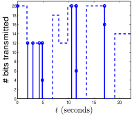
(a)

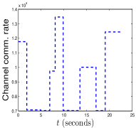
(b)

Figure 1: (a) shows the transmission times, the number of bits transmitted on each transmission and the time-varying function $n\bar{p}$ (dashed line). The three intervals, $(4.88,6.88]$, $(11.52,13.52]$ and $(17.05,19.05]$, with $\bar{p}=0$ are the blackouts. (b) shows the time-varying function $R$.

Figure 2(a) shows the evolution of $V$ and $V_{d}$ and it is clear that the control goal is satisfied. Notice that, just before a blackout, $V$ decreases sharply in anticipation to ensure that the control goal is not violated during the blackout. Figure 2(b) shows the (interpolated) cumulative number of bits transmitted as a function of time. We see that there is a rush of transmissions just prior to $4.88$ units of time, which we see from Figure 1(a) is the beginning of the first blackout.

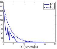
(a)

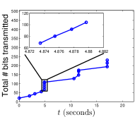
(b)

Figure 2: Evolution of (a) $V$ and $V_{d}$ and (b) total number of bits transmitted, the inset shows that the transmission times are separated.

The number of transmissions in the $20$ units of time in the simulation are $16$, with the average inter-transmission interval as $1.26$ and the minimum as $0.002$. From Figure 2(b), we also see that on an average $11.5$ bits are transmitted per unit time.

7 Conclusions

We have addressed the problem of event-triggered control of linear time-invariant systems under time-varying rate-limited communication channels. The class of time-varying channels we consider is broad enough to include intermittent occurrence of channel blackouts, which are intervals of time when the communication channel is unavailable for feedback. We have designed an event-triggered control scheme that, using prior knowledge of the channel information, guarantees the exponential stabilization of the system at a desired convergence rate, even in the presence of intermittent channel blackouts. Key enablers of our design are the definition and analysis of the data capacity, which measures the maximum number of bits that can be communicated over a given time interval through one or more transmissions. We have also provided an efficient real-time algorithm to lower bound the data capacity for a time-slotted model of channel evolution. An important assumption we make is that the encoder has knowledge of the channel evolution sufficiently ahead of time so that it can plan its transmission schedule. In practice, the channel will have to be estimated, and only uncertain knowledge of its future evolution may be available. Nevertheless, we showed that the problem of estimating the data capacity, which is needed in order to design a meaningful mechanism to guarantee exponential stability, is challenging even assuming full channel information. Future work will explore the reduction of the conservatism of the proposed design, scenarios with bounded disturbances, a stochastic model of channel evolution, and the trade-off between the available information pattern at the encoder and the ability to perform event-triggered control.

References

- Anta and Tabuada [2009] A. Anta and P. Tabuada. On the benefits of relaxing the periodicity assumption for networked control systems over can. In IEEE Real-Time Systems Symposium, pages 3–12, Washington DC, 2009.
- Franceschetti and Minero [2014] M. Franceschetti and P. Minero. Elements of information theory for networked control systems. In G. Como, B. Bernhardsson, and A. Rantzer, editors, Information and Control in Networks, volume 450, pages 3–37. Springer, New York, 2014.
- Garcia and Antsaklis [2013] E. Garcia and P. J. Antsaklis. Model-based event-triggered control for systems with quantization and time-varying network delays. IEEE Transactions on Automatic Control, 58(2):422–434, 2013.
- Heemels et al. [2012] W. P. M. H. Heemels, K. H. Johansson, and P. Tabuada. An introduction to event-triggered and self-triggered control. In IEEE Conf. on Decision and Control, pages 3270–3285, Maui, HI, 2012.
- Keyong and Baillieul [2004] L. Keyong and J. Baillieul. Robust quantization for digital finite communication bandwidth (dfcb) control. IEEE Transactions on Automatic Control, 49(9):1573–1584, 2004.
- Keyong and Baillieul [2007] L. Keyong and J. Baillieul. Robust and efficient quantization and coding for control of multidimensional linear systems under data rate constraints. International Journal on Robust and Nonlinear Control, 17:898–920, 2007.
- Lehmann and Lunze [2010] D. Lehmann and J. Lunze. Event-based control using quantized state information. In IFAC Workshop on Distributed Estimation and Control in Networked Systems, pages 1–6, Annecy, France, September 2010.
- Li et al. [2012] L. Li, X. Wang, and M. D. Lemmon. Stabilizing bit-rate of disturbed event triggered control systems. In Proceedings of the 4th IFAC Conference on Analysis and Design of Hybrid Systems, pages 70–75, Eindhoven, Netherlands, June 2012.
- Liberzon [2003] D. Liberzon. Switching in Systems and Control. Systems & Control: Foundations & Applications. Birkhäuser, 2003. ISBN 0817642978.
- Liberzon [2014] D. Liberzon. Finite data-rate feedback stabilization of switched and hybrid linear systems. Automatica, 50(2):409–420, 2014.
- Martins et al. [2006] N. Martins, M. Dahleh, and N. Elia. Feedback stabilization of uncertain systems in the presence of a direct link. IEEE Transactions on Automatic Control, 51(3):438–447, 2006.
- Minero et al. [2009] P. Minero, M. Franceschetti, S. Dey, and G. N. Nair. Data rate theorem for stabilization over time-varying feedback channels. IEEE Transactions on Automatic Control, 54(2):243–255, 2009.
- Minero et al. [2013] P. Minero, L. Coviello, and M. Franceschetti. Stabilization over Markov feedback channels: the general case. IEEE Transactions on Automatic Control, 58(2):349–362, 2013.
- Nair and Evans [2000] G. N. Nair and R. J. Evans. Stabilization with data-rate-limited feedback: Tightest attainable bounds. Systems & Control Letters, 41(1):49–56, 2000.
- Nair and Evans [2004] G. N. Nair and R. J. Evans. Stabilizability of stochastic linear systems with finite feedback data rates. SIAM Journal on Control and Optimization, 43(2):413–436, 2004.
- Nair et al. [2007] G. N. Nair, F. Fagnani, S. Zampieri, and R. J. Evans. Feedback control under data rate constraints: an overview. Proceedings of the IEEE, 95(1):108–137, 2007.
- Pearson et al. [2014] J. Pearson, J. P. Hespanha, and D. Liberzon. Control with minimum communication cost per symbol. In IEEE Conf. on Decision and Control, pages 6050–6055, Los Angeles, CA, 2014.
- Persis [2005] C. De Persis. -bit stabilization of -dimensional nonlinear systems in feedforward form. IEEE Transactions on Automatic Control, 50(3):299–311, 2005.
- Sun and Wang [2014] Y. Sun and X. Wang. Stabilizing bit-rates in networked control systems with decentralized event-triggered communication. Discrete Event Dynamic Systems, 24(2):219–245, 2014.
- Tabuada [2007] P. Tabuada. Event-triggered real-time scheduling of stabilizing control tasks. IEEE Transactions on Automatic Control, 52(9):1680–1685, 2007.
- Tallapragada and Chopra [2012] P. Tallapragada and N. Chopra. On co-design of event trigger and quantizer for emulation based control. In American Control Conference, pages 3772–3777, Montreal, Canada, June 2012.
- Tallapragada and Cortés [2016] P. Tallapragada and J. Cortés. Event-triggered stabilization of linear systems under bounded bit rates. IEEE Transactions on Automatic Control, 61(7), 2016. To appear.
- Tallapragada et al. [2015] P. Tallapragada, M. Franceschetti, and J. Cortés. Event-triggered stabilization of linear systems under channel blackouts. In Allerton Conf. on Communications, Control and Computing, Monticello, IL, 2015. Submitted.
- Tatikonda and Mitter [2004] S. Tatikonda and S. Mitter. Control under communication constraints. IEEE Transactions on Automatic Control, 49(7):1056–1068, 2004.
- Wang and Lemmon [2011] X. Wang and M. D. Lemmon. Event-triggering in distributed networked control systems. IEEE Transactions on Automatic Control, 56(3):586–601, 2011.