Present address: ]Department of Physics and Astronomy, University of Iowa, Iowa City, IA, USA
Present address: ]Laboratory of Biological Modeling, NIDDK, NIH, Bethesda, Maryland, USA
Fermilab Lattice and MILC Collaborations
from decays and (2+1)-flavor lattice QCD
Abstract
We present a lattice-QCD calculation of the semileptonic form factors and a new determination of the CKM matrix element . We use the MILC asqtad 2+1-flavor lattice configurations at four lattice spacings and light-quark masses down to 1/20 of the physical strange-quark mass. We extrapolate the lattice form factors to the continuum using staggered chiral perturbation theory in the hard-pion and SU(2) limits. We employ a model-independent parameterization to extrapolate our lattice form factors from large-recoil momentum to the full kinematic range. We introduce a new functional method to propagate information from the chiral-continuum extrapolation to the expansion. We present our results together with a complete systematic error budget, including a covariance matrix to enable the combination of our form factors with other lattice-QCD and experimental results. To obtain , we simultaneously fit the experimental data for the differential decay rate obtained by the BaBar and Belle collaborations together with our lattice form-factor results. We find where the error is from the combined fit to lattice plus experiments and includes all sources of uncertainty. Our form-factor results bring the QCD error on to the same level as the experimental error. We also provide results for the vector and scalar form factors obtained from the combined lattice and experiment fit, which are more precisely-determined than from our lattice-QCD calculation alone. These results can be used in other phenomenological applications and to test other approaches to QCD.
pacs:
13.20.He, 12.38.Gc, 12.15.HhI introduction
The Cabibbo-Kobayashi-Masakawa (CKM) matrix Cabibbo:1963yz ; Kobayashi:1973fv element is one of the fundamental parameters of the Standard Model and is an important input to searches for CP violation beyond the Standard Model. Constraints on new physics in the flavor sector are commonly cast in terms of over-constraining the apex of the CKM unitarity triangle. In contrast to the well-determined angle of the unitarity triangle, the opposite side is poorly determined, and the uncertainty is currently dominated by . This is due to the fact that charmless decays of the meson have far smaller branching fractions than the charmed decays, as well as the fact that the theoretical calculations are less precise than for , , or . Currently the most precise determination of is obtained from charmless semileptonic decays, using exclusive or inclusive methods that rely on the measurements of the branching fractions and the corresponding theoretical inputs. Exclusive determinations require knowledge of the form factors, while inclusive determinations rely on the operator product expansion, perturbative QCD, and non-perturbative input from experiments. There is a long standing discrepancy between determined from inclusive and exclusive decays: the central values from these two approaches differ by about . It was argued in Ref. Crivellin:2014zpa that this tension is unlikely to be due to new physics effects, and it is therefore important to examine the (theoretical and experimental) inputs to the determinations. With the result obtained in this paper, the tension is reduced to .
In the limit of vanishing lepton mass, the Standard Model prediction for the differential decay rate of the exclusive semileptonic decay is given by
| (1) |
where is the pion momentum in the -meson rest frame. To determine , the form factor must be calculated with nonperturbative methods. The first unquenched lattice calculations of with 2+1 dynamical sea quarks were performed by HPQCD hep-lat/0601021 and the Fermilab/MILC collaborations 0811.3640 several years ago. Here we extend and improve Ref. 0811.3640 in several ways.
The most recent exclusive determination of from the Heavy Flavor Averaging Group (HFAG) 1207.1158 is based on combined lattice plus experiment fits and yields , where the error includes both the experimental and theoretical uncertainties. The experimental data included in the average are the BaBar untagged six--bin data 1005.3288 , the BaBar untagged twelve--bin data 1208.1253 , the Belle untagged data 1012.0090 , and the Belle hadronic tagged 1306.2781 data. The theoretical errors on the form factors from lattice QCD 0811.3640 are currently the dominant source of uncertainty in 1209.4674 . Hence a new lattice calculation of with improved statistical and systematic errors is desirable 111Note that there are several other efforts with 2 1211.6327 and 2+1 flavors of sea quarks Flynn:2015mha ; 1310.3207 .. To compare, the value of from the inclusive method quoted by HFAG is about 1207.1158 using the theory of Ref. Bosch:2004bt .
In this paper, we present a new lattice-QCD calculation of the semileptonic form factors and a determination of . Our calculation shares some features with the previous Fermilab/MILC calculation 0811.3640 but makes several improvements. We quadruple the statistics on the previously used ensembles and improve our strategy for extracting the form factors by including excited states in our three-point correlator analysis. In addition, we include twice as many ensembles in this analysis. The new ensembles have smaller lattice spacings, with the smallest lattice spacing decreased by half. This analysis also includes ensembles with light sea-quark masses that are much closer to their physical values ( versus ). The smaller lattice spacings and light-quark masses provide much better control over the dominant systematic error due to the chiral-continuum extrapolation. We find that heavy-meson rooted staggered chiral perturbation theory (HMrSPT) in the SU(2) and hard-pion limits provides a satisfactory description of our data. All together, these improvements reduce the error on the form factors by a factor of about 3. Finally, we introduce a new functional method for the extrapolation over the full kinematic range.
The determination of from a combined fit to our lattice form factors together with experimental measurements also yields a very precise determination of the vector and scalar form factors over the entire kinematic range. These form factors will be valuable input to other phenomenological applications in the Standard Model and beyond. An example is the rare decay , which we will discuss in a separate paper.
Because our primary goal in this work was a reliable and precise determination of , we employed a blinding procedure to minimize subjective bias. At the stage of matching between the lattice and continuum vector currents, a slight multiplicative offset was applied to the data that was only known to two of the authors. The numerical value of the blinding factor was only disclosed after the analysis and error-estimation procedure, including the determination of , were essentially finalized.
This paper is organized as follows. In Sec. II, we present our calculation of the form factors. We describe the lattice actions, currents, simulation parameters, correlation functions and fits to extract the matrix elements, renormalization of the currents, and adjustment of the form factors to correct for quark-mass mistunings. In Sec. III, we present the combined chiral-continuum extrapolation, followed by an itemized presentation of our complete error budget in Sec. IV. We then extrapolate the form factors to the full range through the functional expansion method in Sec. V. We also perform fits to lattice and experimental data simultaneously, to obtain . We conclude with a comparison to other results and discussion of the future outlook in Sec. VI. Preliminary reports of this work can be found in Refs. Du:2013kea ; Bailey:2014fpx .
II Lattice-QCD simulation
In this section, we describe the details of the lattice simulation. We briefly describe the calculation of the form factors in Sec. II.1. We also calculate the tensor form factor, which follows a analysis similar to that of the vector and scalar form factors. The tensor form factor enters the Standard-Model rate for decay, and our final result for will be presented in a forthcoming paper. In Sec. II.2, we introduce the actions and simulation parameters used in this analysis. This is followed, in Sec. II.3, by a brief discussion of the currents and lattice correlation functions. The correlator fits to extract the lattice form factors are provided in Sec. II.4. In Sec. II.5, we discuss the renormalization of the lattice currents. In Sec. II.6, we correct the form factors a posteriori to account for the mistuning of the simulated heavy -quark mass.
II.1 Form-factor definitions
The vector and tensor hadronic matrix elements relevant for semileptonic decays can be parameterized by the following three form factors:
| (2) | |||||
| (3) |
where , and . In lattice gauge theory and in chiral perturbation theory, it is convenient to parameterize the vector-current matrix elements by hep-ph/0101023
| (4) |
where is the four velocity of the meson and is the projection of the pion momentum in the direction perpendicular to . The pion energy is related to the lepton momentum transfer by . With this setup, we have
| (5) | |||||
| (6) | |||||
| (7) |
where no summation is implied by the repeated indices here. The form factors and are
| (8) | |||||
| (9) |
II.2 Actions and parameters
The lattice gauge-field configurations we use have been generated by the MILC Collaboration 0903.3598 ; Bernard:2001av ; Aubin:2004wf , and some of their properties are listed in Table 1. These twelve ensembles have four different lattice spacings ranging from fm to fm with several light sea-quark masses at most lattice spacings in the range . The parameter range is shown in Fig. 1. We use the Symanzik-improved gauge action Weisz:1982zw ; Weisz:1983bn ; Luscher:1984xn for the gluons and the tadpole-improved (asqtad) staggered action hep-lat/9609036 ; Lepage:1998vj ; hep-lat/9806014 ; hep-lat/9805009 ; hep-lat/9903032 ; hep-lat/9912018 for the 2+1 flavors of dynamical sea quarks and for the light valence quarks. Both Table 1 and Fig. 1 also indicate the ensembles used in the previous Fermilab/MILC calculation 0811.3640 . The current analysis benefits from an almost quadrupled increase in the statistics over that of Ref. 0811.3640 , as well as finer lattice spacings and lighter sea-quark masses. All ensembles have large enough spatial volume, , such that the systematic error due to finite-size effects is negligible compared to other uncertainties.
| (fm) | volume | (Ref. 0811.3640 )) | |||||
| 0.12 | 0.01/0.05 | 6.760 | 0.8677 | 2259 | 4.5 | 592 | |
| 0.007/0.05 | 6.760 | 0.8678 | 2110 | 3.8 | 836 | ||
| 0.005/0.05 | 6.760 | 0.8678 | 2099 | 3.8 | 529 | ||
| 0.09 | 0.0062/0.031 | 7.090 | 0.8782 | 1931 | 4.1 | 557 | |
| 0.00465/0.031 | 7.085 | 0.8781 | 984 | 4.1 | |||
| 0.0031/0.031 | 7.080 | 0.8779 | 1015 | 4.2 | |||
| 0.00155/0.031 | 7.075 | 0.877805 | 791 | 4.8 | |||
| 0.06 | 0.0072/0.018 | 7.480 | 0.8881 | 593 | 6.3 | ||
| 0.0036/0.018 | 7.470 | 0.88788 | 673 | 4.5 | |||
| 0.0025/0.018 | 7.465 | 0.88776 | 801 | 4.4 | |||
| 0.0018/0.018 | 7.460 | 0.88764 | 827 | 4.3 | |||
| 0.045 | 0.0028/0.014 | 7.810 | 0.89511 | 801 | 4.6 |
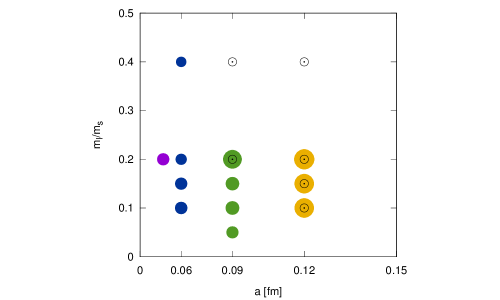
In this calculation, we work in the full-QCD limit, so that the light valence-quark masses are the same as the light sea-quark masses , which are degenerate. For the bottom quarks, we use the Fermilab interpretation hep-lat/9604004 of the Sheikholeslami-Wohlert clover action Sheikholeslami:1985ij . In Table 2, we list parameters for the valence quarks.
| (fm) | ||||||
| 0.12 | 0.01/0.05 | 1.531 | 0.0901 | 0.09334 | 4 | 18,19 |
| 0.007/0.05 | 1.530 | 0.0901 | 0.09332 | 4 | 18,19 | |
| 0.005/0.05 | 1.530 | 0.0901 | 0.09332 | 4 | 18,19 | |
| 0.09 | 0.0062/0.031 | 1.476 | 0.0979 | 0.09677 | 4 | 25,26 |
| 0.00465/0.031 | 1.477 | 0.0977 | 0.09671 | 4 | 25,26 | |
| 0.0031/0.031 | 1.478 | 0.0976 | 0.09669 | 4 | 25,26 | |
| 0.00155/0.031 | 1.4784 | 0.0976 | 0.09669 | 4 | 25,26 | |
| 0.06 | 0.0072/0.018 | 1.4276 | 0.1048 | 0.09636 | 4 | 36,37 |
| 0.0036/0.018 | 1.4287 | 0.1052 | 0.09631 | 4 | 36,37 | |
| 0.0025/0.018 | 1.4293 | 0.1052 | 0.09633 | 4 | 36,37 | |
| 0.0018/0.018 | 1.4298 | 0.1052 | 0.09635 | 4 | 36,37 | |
| 0.045 | 0.0028/0.014 | 1.3943 | 0.1143 | 0.08864 | 4 | 48,49 |
Table 3 lists the values of on each ensemble, along with other derived parameters, where is the characteristic distance between two static quarks such that the force between them satisfies hep-lat/0002028 ; hep-lat/9310022 . The absolute lattice scale is obtained by comparing the Particle Data Group value of with lattice calculations of from MILC 0910.2966 and HPQCD 0910.1229 , yielding the absolute scale fm 1112.3051 . This value is consistent with the independent, but less precise, determination from RBC/UKQCD using domain-wall fermions Arthur:2012opa .
| (fm) | (MeV) | (MeV) | |||
| 0.12 | 0.01/0.05 | 2.7386 | 389 | 532 | 0.14091 |
| 0.007/0.05 | 2.7386 | 327 | 488 | 0.14095 | |
| 0.005/0.05 | 2.7386 | 277 | 456 | 0.14096 | |
| 0.09 | 0.0062/0.031 | 3.7887 | 354 | 413 | 0.139119 |
| 0.00465/0.031 | 3.7716 | 307 | 374 | 0.139134 | |
| 0.0031/0.031 | 3.7546 | 249 | 329 | 0.139173 | |
| 0.00155/0.031 | 3.7376 | 177 | 277 | 0.139190 | |
| 0.06 | 0.0072/0.018 | 5.3991 | 450 | 466 | 0.137582 |
| 0.0036/0.018 | 5.3531 | 316 | 340 | 0.137632 | |
| 0.0025/0.018 | 5.3302 | 264 | 291 | 0.137667 | |
| 0.0018/0.018 | 5.3073 | 224 | 255 | 0.137678 | |
| 0.045 | 0.0028/0.014 | 7.2082 | 324 | 331 | 0.136640 |
II.3 Currents and correlation functions
We calculate the two-point and three-point functions
| (10) | |||||
| (11) |
where , labels the pseudoscalar meson, the operators () annihilate (create) the states with the quantum numbers of the pseudoscalar meson on the lattice, and are the lattice currents.
For the meson, we use a mixed-action interpolating operator which is a combination of a Wilson clover bottom quark and a staggered light quark 0811.3640 :
| (12) |
where , , and is a smearing function. For the pion, we use the operator
| (13) |
which is constructed from two 1-component staggered quarks.
The current operators are constructed in a similar way:
| (14) | |||||
| (15) |
where the heavy quark field spinor is rotated to remove tree-level discretization effects, via hep-lat/9604004
| (16) |

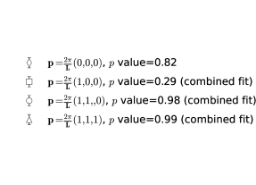
Figure 2 illustrates the three-point correlation function used to obtain the lattice form factors. The current operator is inserted between the - and -quark lines. The three-point functions depend on both the current insertion time and the temporal separation between the and mesons. The signal to noise ratio is largely determined by . A convenient approach is to fix the source-sink separation in the simulations and then insert the current operators at every time slice in between. The source-sink separations at different lattice spacings, sea-quark masses, and recoil momenta are chosen to be approximately the same in physical units. To minimize statistical uncertainties and reduce excited-state contamination, we tested data with different source-sink separations before choosing those shown in Table 2. The meson is at rest in our simulation, while the daughter pion is either at rest or has a small three-momentum. The light-quark propagator is computed from a point source so that one inversion of the Dirac operator can be used to obtain multiple momenta. The spatial source location is varied randomly from one configuration to the next to minimize autocorrelations. The -quark source is always implemented with smearing based on a Richardson 1S wave function menscher2005 after fixing to Coulomb gauge. We compute both the two-point function and three-point function at several of the lowest possible pion momenta in a finite box: , , , and , where contributions from each momentum are averaged over permutations of components. We find the correlation functions with momentum too noisy to be useful, so we exclude these data from our analysis.
II.4 Two-point and three-point correlator fits
In this subsection, we describe how to extract the desired matrix element from two- and three-point correlation functions. With our choice for the valence-quark actions and for the interpolating operators, the two- and three-point functions take the form hep-lat/0211014
| (17) | |||||
where is the temporal length of the lattice and
| (19) | |||||
| (20) |
Note that due to the staggered action used for the light quarks, the meson interpolating operators also couple to the positive parity (scalar) states which oscillate in Euclidean times and with the factors and .
Our goal is to extract , the ground state matrix element from these correlation functions. To suppress the contributions from the positive parity states to the ratio, we follow the averaging procedure of Ref. 0811.3640 , which exploits the oscillating sign in their Euclidean time dependence. The time averages can be thought of as a smearing over neighboring time slices to significantly reduce the overlap with opposite-parity states. Denoting the averaged correlators by and , we then use the ratio 0811.3640
| (21) |
where and are the ground-state pion energy and -meson rest mass, respectively. The uncertainty in the -meson rest mass has significant impact on the ratio , so we follow a two-step procedure. We first determine the pion and -meson ground-state energy as precisely as possible using the corresponding two-point functions. We then feed these ground-state energies into the ratio , preserving the correlations with jackknife resampling.
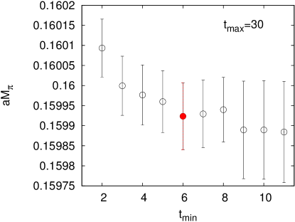
For the pion two-point functions at zero momentum, the oscillating states — the terms in Eq. (17) with odd powers of — do not appear. Thus, we fit the pion two-point functions using Eq. (17) with the lowest two non-oscillating states (). For the two-point functions with nonzero momentum, the contribution from oscillating states is small but noticeable. We find that we only need to include the lowest three states ( in the fits. Because the momenta we consider are typically small compared to , the continuum dispersion relation is satisfied within statistical errors, as shown in Fig. 3. In the main analysis, we therefore use the mass from the zero-momentum fit and the continuum dispersion relation to set for non-zero momentum. Because the zero-momentum energy has significantly smaller statistical error than that of nonzero momentum, using this choice and the dispersion relation for nonzero-momentum energy leads to a more stable and precise determination of . Table 4 lists the relevant fit ranges for the two-point fits. In the two-point correlators (except the zero-momentum pion two-point correlators), the noise grows rapidly with increasing , the distance away from the pion source in the temporal direction. The data points at large are not useful, and including them would lead to a larger covariance matrix which would be difficult to resolve given the limited number of configurations. We choose the upper end of the fit ranges such that the relative error does not exceed 20%. The lower end is chosen such that the excited state contamination is sufficiently small, i.e., the resulting central values of the ground state energy are stable against variations in as shown in Fig. 4 (left).


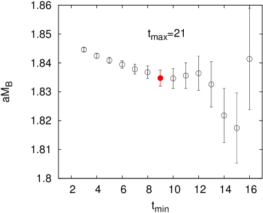
In our analysis, there are two places where quantities from the -meson two-point functions are needed. The first is for in Eq. (21). The second is for the -meson excited state energy in Eq. (22) below. For the determination of in Eq. (21) we use two-point functions constructed with a 1S-smearing function in the interpolating operators for the source and sink. The 1S-smeared operator has good overlap with the ground state and a much smaller overlap with the excited states than the local source operator, thus reducing excited-state contributions to the corresponding correlators. We fit the 1S-1S smeared -meson two-point correlators with relatively large to only two states ( in Eq. (17)). To choose , we again apply the 20%-rule on the relative error. The lower bound is chosen in a manner similar to the pion two-point fits and the stability plot is shown in Fig. 4 (right). The chosen fit ranges are shown in Table 4.
| (fm) | (2+0) | (1+1) | |
| 0.12 | 0.01/0.05 | [6, 30] | [9, 21] |
| 0.007/0.05 | [6, 30] | [9, 21] | |
| 0.005/0.05 | [6, 30] | [9, 21] | |
| 0.09 | 0.0062/0.031 | [9, 47] | [12, 32] |
| 0.00465/0.031 | [9, 47] | [12, 29] | |
| 0.0031/0.031 | [9, 47] | [13, 29] | |
| 0.00155/0.031 | [9, 47] | [14, 29] | |
| 0.06 | 0.0072/0.018 | [13, 71] | [14, 41] |
| 0.0036/0.018 | [13, 71] | [14, 41] | |
| 0.0025/0.018 | [13, 71] | [14, 41] | |
| 0.0018/0.018 | [13, 71] | [15, 41] | |
| 0.045 | 0.0028/0.014 | [17, 74] | [17, 61] |
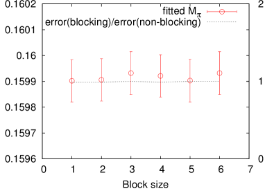
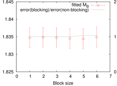
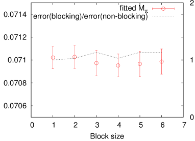
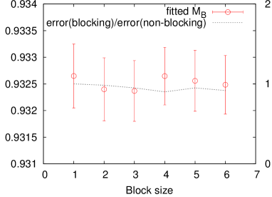
We test for autocorrelations by blocking the configurations on each ensemble with different block sizes, and then using a single-elimination jackknife procedure to propagate the statistical error to the two-point correlator fits for and . We do not observe any noticeable autocorrelations in all the ensembles we use, as illustrated in Fig. 5 for the coarsest and finest ensembles, and choose not to block the data.
The ratios in Eq. (21) have the advantage that the wavefunction overlap factors cancel, but the trade-off is that we need an additional factor — the square root term on the right-hand side — to remove the leading dependence in the ratio. If the lowest lying states dominated the ratio , then it would be constant in and proportional to the lattice form factor . The subscript now runs over , , and , corresponding to the operators , , and , respectively. Our previous analysis employed a simple plateau fit constant in time. With our improved statistics, the small excited-state contributions to the ratio are significant and cannot be neglected. On the other hand, even with our improved statistics, we find that contributions to from wrong-parity states are still negligible. We use two different fit strategies to remove excited state contributions and use the consistency between them as an added check that any remaining excited state contamination is negligibly small.
The first strategy starts with the ratio in Eq. (21) and minimally extends the plateau fitting scheme by including the first excited state of the meson in the following form:
| (22) |
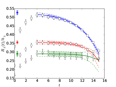
where and are unconstrained fit parameters, is the lowest energy splitting of the pseudoscalar meson, and the prefactors are and . We choose the fit ranges for such that contributions from pion excited states to can be neglected. The fit parameter is determined by the -meson two-point correlators. In practice, we fit the ratio in Eq. (22) along with the -meson two-point correlation functions with as a common parameter. We find it beneficial in the combined fit to include both the local and smeared two-point correlation functions. We use 2+2 states for both correlators, but use a different set of fit ranges (listed in Table 5). The results of these two-point fits are shown in Fig. 6. The agreement in the -meson energies between the separate and combined fits is very good, but the combined fit leads to smaller errors.

| (fm) | ||||||
| 0.12 | 0.01/0.05 | [9, 23] | [7, 21] | [6,12] | [6,12] | [6,12] |
| 0.007/0.05 | [9, 23] | [7, 21] | [6,12] | [6,12] | [6,12] | |
| 0.005/0.05 | [9, 23] | [7, 21] | [6,12] | [6,12] | [6,12] | |
| 0.09 | 0.0062/0.031 | [12, 32] | [9, 32] | [9,16] | [9,16] | [9,16] |
| 0.00465/0.031 | [12, 32] | [9, 29] | [9,16] | [9,16] | [9,16] | |
| 0.0031/0.031 | [12, 32] | [9, 29] | [9,16] | [9,16] | [9,16] | |
| 0.00155/0.031 | [12, 29] | [9, 29] | [9,15] | [9,15] | [9,15] | |
| 0.06 | 0.0072/0.018 | [13, 41] | [9, 41] | [12,22] | [12,22] | [12,22] |
| 0.0036/0.018 | [13, 41] | [9, 41] | [12,22] | [12,22] | [12,22] | |
| 0.0025/0.018 | [13, 41] | [9, 41] | [12,22] | [12,22] | [12,22] | |
| 0.0018/0.018 | [13, 41] | [9, 41] | [12,21] | [12,21] | [12,21] | |
| 0.045 | 0.0028/0.014 | [16, 61] | [10, 61] | [16,26] | [16,26] | [16,26] |
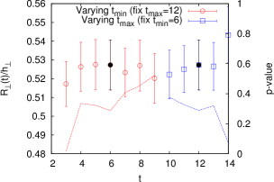
To summarize our strategy, for the case of zero momentum, we fit the ratio together with the local and smeared -meson two-point correlators , simultaneously. For non-zero momentum , is common to all three ratios, . Thus, we perform a combined fit to the five quantities: and . Figure 7 shows an example of these fits. Figure 8 shows the stability plots of against the variations in the fit ranges of the ratio fits, and the variations in the fit ranges of both two-point correlators. The preferred fit ranges are set to be in the stable region upon these variations.
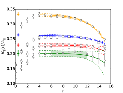
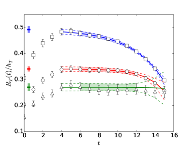
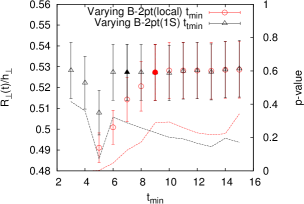
Our second fit strategy includes excited-state contributions from both the pion and the meson. It starts with a different ratio, without time averages, which ensures that there are enough data points to constrain all the parameters:
| (23) |
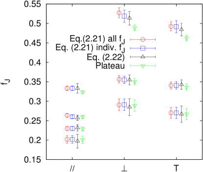
where the two- and three-point correlators are defined in Eqs. (10) and (11). We fit with all the possible states with in Eqs. (17) and (LABEL:eq:C_3pt), combining the fits to the pion and -meson two-point correlators. We compare the fit results of the two different fit schemes in Fig. 9. The first (simple) fit model described in Eq. (22) gives, fitting either simultaneously or individually to the three lattice form factors , results that are consistent with the second fit model that includes the full set of first excited states in Eq. (23). In contrast, the plateau fits to defined in Eq. (21) yield results that are as much as one statistical smaller. In summary, we find that the first fit strategy described by Eq. (22) is sufficient to remove contributions from excited states, and we therefore adopt this method for the main analysis.
II.5 Matching
We match the lattice currents to continuum QCD with the relation,
| (24) |
where and denote the vector or tensor currents in the continuum and lattice theories, respectively, and “” means “has the same matrix elements” Kronfeld:2000ck . We calculate the current renormalization with the mostly nonperturbative renormalization method hep-ph/0101023 ; Harada:2001fi ,
| (25) |
where and are the matching factors for the corresponding flavor-conserving vector currents. These factors capture most of the current renormalization. The remaining flavor off-diagonal contribution to the matching factor, , is close to unity.
We calculate the factors and nonperturbatively for each ensemble by computing the matrix elements of the flavor-conserving vector currents and using the relations
| (26) | |||||
| (27) |
where the lattice current is a bilinear of light staggered quark fields and is a bilinear of clover heavy quark fields. The factors and are listed in Table 6. Because there is very little dependence in the factor , we use the same for ensembles with different light quark masses but the same lattice spacing. The factor depends crucially on the heavy quark mass, though it has negligible light quark mass dependence.
We use lattice perturbation theory hep-lat/9209022 to compute the remaining renormalization factors at one-loop. Due to the cancellation of the tadpole contributions in the radiative corrections to the left and right side of Eq. (25), the factors are very close to one. They have the perturbative expansion
| (28) |
where we take the strong coupling in the -scheme hep-lat/9209022 at a scale that corresponds to the typical gluon loop momentum. In practice, we choose . The details of the calculation of the one-loop coefficients will be presented elsewhere. The values used in this work are shown in Table 6.
| (fm) | |||||||
|---|---|---|---|---|---|---|---|
| 0.12 | 0.01/0.05 | 0.0901 | 0.5015(8) | 1.741(3) | 1.006214 | 0.973023 | 1.033350 |
| 0.007/0.05 | 0.0901 | 0.5015(8) | 1.741(3) | 1.006252 | 0.973109 | 1.033280 | |
| 0.005/0.05 | 0.0901 | 0.5015(8) | 1.741(3) | 1.006197 | 0.973082 | 1.033270 | |
| 0.01/0.05 | 0.0860 | 0.5246(9) | 1.741(3) | 1.012999 | 0.977290 | 1.030650 | |
| 0.01/0.05 | 0.0820 | 0.5469(10) | 1.741(3) | 1.018261 | 0.980129 | 1.028960 | |
| 0.09 | 0.0062/0.031 | 0.0979 | 0.4519(15) | 1.776(5) | 0.999308 | 0.975822 | 1.036590 |
| 0.00465/0.031 | 0.0977 | 0.4530(15) | 1.776(5) | 0.999405 | 0.975775 | 1.036390 | |
| 0.0031/0.031 | 0.0976 | 0.4536(15) | 1.776(5) | 0.999441 | 0.975744 | 1.036350 | |
| 0.00155/0.031 | 0.0976 | 0.4536(15) | 1.776(5) | 0.999416 | 0.975703 | 1.036390 | |
| 0.06 | 0.0072/0.018 | 0.1048 | 0.4089(21) | 1.807(7) | 0.995605 | 0.979279 | 1.042390 |
| 0.0036/0.018 | 0.1052 | 0.4065(21) | 1.807(7) | 0.995371 | 0.979260 | 1.043160 | |
| 0.0025/0.018 | 0.1052 | 0.4065(21) | 1.807(7) | 0.995350 | 0.979217 | 1.043190 | |
| 0.0018/0.018 | 0.1052 | 0.4065(21) | 1.807(7) | 0.995327 | 0.979176 | 1.043250 | |
| 0.045 | 0.0028/0.014 | 0.1143 | 0.3564(65) | 1.841(6) | 0.994195 | 0.984351 | 1.058790 |
II.6 Heavy-quark mass correction
In the clover action, the hopping parameter corresponds to the bare -quark mass. When we started generating data for this analysis, we had a good estimate for the bottom-quark on each ensemble, but not the final tuned values, which were obtained as described in Appendix C of Ref. Bailey:2014tva . We therefore need to adjust the form factors a posteriori to account for the slightly mistuned values of .
The parameters are adjusted so that the corresponding kinetic masses match the experimentally-measured value Bailey:2014tva . Table 7 shows both the simulation and final tuned values. For some ensembles, the difference between the two is as large as 7 of the statistical uncertainty associated with the tuning procedure. We study the -dependence of the lattice form factors by generating data on the fm, ensemble, with two additional values, and , and all other simulation parameters unchanged.
| (fm) | (%) | (%) | (%) | (%) | |||
| 0.12 | 0.01/0.05 | 0.0901 | 0.0868(9) | 10.9 | 1.79 | 1.55 | 1.60 |
| 0.007/0.05 | 0.0901 | 0.0868(9) | 10.9 | 1.80 | 1.57 | 1.58 | |
| 0.005/0.05 | 0.0901 | 0.0868(9) | 10.9 | 1.81 | 1.58 | 1.56 | |
| 0.09 | 0.0062/0.031 | 0.0979 | 0.0967(8) | 4.3 | 0.69 | 0.60 | 0.62 |
| 0.00465/0.031 | 0.0977 | 0.0966(8) | 3.9 | 0.63 | 0.55 | 0.56 | |
| 0.0031/0.031 | 0.0976 | 0.0965(8) | 3.9 | 0.64 | 0.56 | 0.55 | |
| 0.00155/0.031 | 0.0976 | 0.0964(8) | 4.2 | 0.70 | 0.61 | 0.59 | |
| 0.06 | 0.0072/0.018 | 0.1048 | 0.1054(5) | 2.4 | 0.37 | 0.36 | 0.44 |
| 0.0036/0.018 | 0.1052 | 0.1052(5) | 0.0 | 0.0 | 0.0 | 0.0 | |
| 0.0025/0.018 | 0.1052 | 0.1051(5) | 0.4 | 0.06 | 0.06 | 0.06 | |
| 0.0018/0.018 | 0.1052 | 0.1050(5) | 0.8 | 0.13 | 0.11 | 0.11 | |
| 0.045 | 0.0028/0.014 | 0.1143 | 0.1116(4) | 14.3 | 2.34 | 2.03 | 2.10 |
To generalize the dependence from this ensemble to others, we work with the quark kinetic mass instead of itself. We expand the form factor ( in about a reference point (which corresponds to the tuned ) as follows
| (29) | |||||
where the masses and are all in units. To obtain at the reference point, we need to find the dimensionless normalized slope .
We use exactly the same procedure as described in Sec. II.4 for to obtain the form factors for the additional values and . We apply the matching factors given in Table 6. Finally, we take to be the kinetic mass corresponding to (the tuned kappa given in Table 7) and use it as the reference point. We fit each form factor at each momentum for the three data points to the linear form given in Eq. (29), taking and as fit parameters. The result is shown in Fig. 10 (left). As shown in the plot, the normalized slope has a very mild dependence. Therefore, for each form factor we perform a correlated fit to all momenta to obtain a single common normalized slope. The result is shown in Table 8. Fitting the data to a linear form in results in a slope statistically consistent with zero.
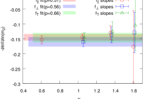
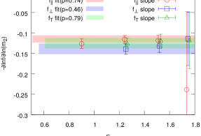
To examine the light-quark mass dependence of the normalized slopes, we repeat the same procedure for the semileptonic form factors with a heavier daughter valence quark , which is close to the physical strange-quark mass. The results are plotted in Fig. 10 (right). We fit the points of each form factor to a constant and tabulate the results in Table 8. Comparing the normalized slopes for and , taking into account statistical correlations, we observe a mild but statistically-significant light daughter-quark mass dependence. So we fit the slopes for and simultaneously to a linear form,
| (30) |
where and for and , respectively. The results for the parameters and are given in Table 8. Note that the results in Table 8 are also used in Ref. ranzhou .
| Combined fit with dependence | |||||||
|---|---|---|---|---|---|---|---|
| value | value | value | |||||
| 0.56 | 0.145(11) | 0.46 | 0.115(9) | 0.4 | 0.146(11) | 0.032(3) | |
| 0.51 | 0.160(16) | 0.74 | 0.139(13) | 0.84 | 0.165(17) | 0.025(8) | |
| 0.66 | 0.146(16) | 0.79 | 0.126(13) | 0.88 | 0.137(17) | 0.034(8) | |
We use the parameters and in Table 8 to determine the normalized slope for each ensemble. Although the dependence of the normalized slopes on the light daughter-quark mass is resolvable, the effects are small for the ensembles we use in the analysis (with light daughter-quark masses ranging from to ). We expect similarly small effects from the spectator-quark masses. We also expect that the lattice-spacing dependence of the normalized slopes is small, because it is a dimensionless ratio. We therefore correct each lattice form factor in each ensemble by a factor
| (31) |
where and are the kinetic masses corresponding to the simulation and tuned , respectively. The resulting relative shift for each ensemble is shown in Table 7. Although the corrections to itself are significant for some ensembles, the corresponding corrections to the form factors are much smaller (), as a consequence of the small normalized slopes.
III Chiral-continuum extrapolation
Here we extrapolate the form factors at four lattice spacings with several unphysical light-quark masses to the continuum limit and physical light-quark mass. We use heavy-meson rooted staggered chiral perturbation theory (HMrSPT) 0704.0795 ; Aubin:2005aq , in the hard-pion and SU(2) limits. We also incorporate heavy-quark discretization effects into the chiral-continuum extrapolation.
III.1 SU(2) staggered chiral perturbation theory in the hard-pion limit
The full-QCD next-to leading order (NLO) HMrSPT expression for the semileptonic form factors can be written 0704.0795
| (32) |
where . Note that the expressions are in units of the mass-independent scale and the coefficients have the dimension of . The leading-order terms are
| (33) | |||||
| (34) |
with the coupling constant and the mass splitting. The terms and are the one-loop nonanalytic contributions in the chiral expansion, and depend upon the light pseudoscalar meson mass and energy 0704.0795 . Note that in the heavy-quark expansion is proportional to up to . We therefore use the same pole location and nonanalytic corrections for as . The terms analytic in are introduced to cancel the scale dependence arising from the nonanalytic contribution in Eq. (32). The dimensionless variables are proportional to the quark mass, pion energy, and lattice spacing. We define
| (35) | |||||
| (36) | |||||
| (37) | |||||
| (38) |
Note that the valence mass is equal to the sea mass in our data. The low-energy constant relates the pseudoscalar meson masses to the quark masses,
| (39) |
and is the mass splitting for staggered taste . The average taste splitting in Eq. (38) is . The quantities and are obtained from the MILC Collaboration’s analysis of light pseudoscalar mesons and are shown in Table 9.
We constrain the parameter with a prior. The value of has been calculated with lattice QCD in the static limit 1109.2480 ; 1203.3378 or with a relativistic quark Flynn:2013kwa on gauge fields generated with domain-wall or Wilson sea quarks 1011.4393 . We set the prior, based on these lattice-QCD calculations, to be , where the error covers the differences among different determinations of the coupling. The LO and NLO coefficients, , are well determined by the data. Note that the formula given in Eq. (32) is slightly different from that in Ref. 0811.3640 where the NLO coefficients therein are our (). With the introduction of variables defined in Eqs. (35)-(38), we should expect that (), or . In the actual fits, and . Note that the coefficients are dimensionful, and they are evaluated here in units. We constrain them with loose priors: and .
Standard HMrSPT uses the assumption that the external and loop pions are soft, i.e., hep-lat/0305001 ; 0710.3496 . In our work, however, the external pion energies can be quite large, in some cases as much as 7 times the physical pion mass, and standard HMrSPT may not converge well enough in this range. Indeed, the fit of the lattice form factor to Eq. (32) gives a poor confidence level (), which is not improved by including higher-order contributions in the chiral expansion. Bijnens and Jemos 1006.1197 proposed an approach called hard-pion PT, in which the internal energetic pions are integrated out and the dependence is absorbed into the low energy constants. 222The factorization of hard-pion PT breaks down starting at three loops Colangelo:2012ew , but we only use the one-loop non-analytic terms. Since hard-pion PT provides a more appropriate description of our data, we adopt it in this analysis. The explicit expressions for the hard-pion nonanalytic terms using SU(3) chiral perturbation theory as well as its SU(2) limit are given in the appendix of Ref. ranzhou . We take the SU(2) limit by integrating out the strange quark. The resulting expression has no explicit strange-quark mass dependence, which has been absorbed into the value of the low energy constants. The SU(2) hard-pion PT provides a better description of our data than the SU(3) hard-pion PT ( value versus from the NLO PT fit with priors). We also find that the chiral expansion converges faster using SU(2) PT when including higher-order chiral corrections in the fit to our data, which results in smaller PT truncation errors than from using SU(3) PT. Finally, Ref. 0710.3496 provides phenomenological arguments to prefer the application of SU(2) HMPT over SU(3) to lattice-QCD data. We therefore use the SU(2) formula for our central value fit, but also check the consistency with the SU(3) fits in Sec. IV.
Based on the above discussion, we use the following conditions for and in Eq. (32):
| (40) | |||||
| (41) | |||||
| (42) | |||||
| (43) |
where Eq. (41) is a consequence of the hard-pion limit, Eq. (42) and the factor 2 in the first term of Eq. (43) follow from the fact that we take and has been integrated out, Eq. (43) preserves the chiral scale independence of the SU(2) hard-pion NLO expression, and is the taste splitting of the taste-singlet pseudoscalar meson mass.
| (fm) | 0.12 | 0.09 | 0.06 | 0.045 | 0 | |
| 0 | 0 | 0 | 0 | 0 | ||
| 0.22705 | 0.07469 | 0.02635 | 0.01041 | 0 | ||
| 0.36616 | 0.12378 | 0.04298 | 0.01698 | 0 | ||
| 0.48026 | 0.15932 | 0.05744 | 0.22692 | 0 | ||
| 0.60082 | 0.22065 | 0.07039 | 0.02781 | 0 | ||
| 0.0 | 0.0 | 0.0 | 0.0 | 0 | ||
| 0 | ||||||
| 6.83190 | 6.63856 | 6.48665 | 6.41743 | 6.015349 |
The fits of the lattice form factors using NLO SU(2) hard-pion HMrSPT have acceptable confidence levels. We find, however, that there is a sizable shift in the fit result when including higher-order terms in the PT expansion. We therefore need to study the effects of higher-order contributions in the chiral expansion.
III.2 Next-to-next-to-leading order (NNLO) corrections
We supplement the NLO SU(2) hard-pion PT expression with the following NNLO analytic terms
| (44) | |||||
such that the complete NNLO PT expression is,
| (45) |
Note that here uses the hard-pion and SU(2) PT, as manifested in Eqs. (40)-(43). All light-quark discretization errors that arise from taste violations are included here; generic errors from light-quark and gluon action, which are , are discussed in Sec. III.3.
Again, the expectation from chiral perturbation theory is that the coefficients of these analytic terms should satisfy when written in terms of the dimensionless variables given in Eqs. (35)–(38). We set the priors for the NNLO coefficients for , , to be , since the role of these terms is simply to absorb the effects of higher-order contributions in the chiral expansion. This width 0.6 corresponds to the size of . For the same reason, we set the priors for the coefficients for , , to be . Doubling the prior widths leads to negligible shifts on the central values of the form factors and less than 20% increases in the fit errors.
III.3 Heavy-quark discretization effects
The chiral-continuum extrapolation implemented in Eq. (45) accounts for the discretization effects from the gluons and the light staggered quarks. Discretization effects from the heavy quark need a separate treatment. Heavy-quark discretization errors arise from the short-distance mismatch of higher-dimension Lagrangian and current operators Kronfeld:2000ck ; Harada:2001fi . By power counting, such mismatches are of or where is a QCD scale appropriate for the heavy-quark expansion. We follow the same method for incorporating the heavy-quark discretization effects described in Ref. 1112.3051 and include the following error function in Eq. (32),
| (46) |
where the mismatch functions are given in the Appendix of Ref. 1112.3051 . The error functions arise from mismatches of operators in the Lagrangian, while functions arise from those of the vector current. The last term in Eq. (46) accounts for higher order heavy-quark and generic light-quark and gluon errors not included in Eq. (45), which is of the order . The fit parameters are constrained with priors: for and for ; the latter two are wider because the functions and both appear twice Harada:2001fi .
To summarize, after incorporating the heavy-quark discretization effects, the complete NNLO SU(2) hard-pion HMrSPT expression is
| (47) |
where is defined in Eq. (45). With this treatment, the uncertainty due to truncating the chiral expansion at NNLO (cf. Sec. IV below), NNLO light-quark and gluon discretization effects, and LO heavy-quark discretization effects are incorporated in the fit error of the chiral-continuum extrapolation. The fits for , , and to Eq. (47) are shown in Fig. 11.
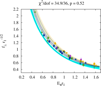
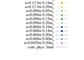
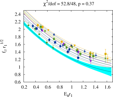
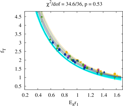
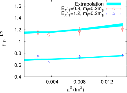
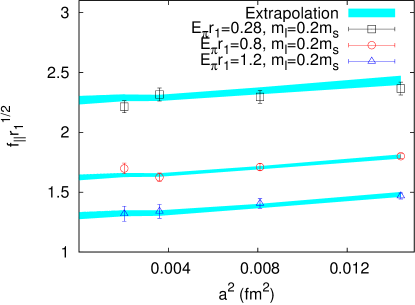
To examine the size of discretization effects, we plot the form factors and with light-quark mass at each lattice spacing versus in Fig. 12. As we can see from the plots, the observed lattice-spacing dependence is very mild, with the data points at the largest lattice spacing ( fm) only about two statistical sigma away from the continuum limit.
IV Systematic error budget
The error output from the central-value fit described in Sec. III.3 already includes the systematic errors due to the light- and heavy-quark discretization effects and the uncertainty on . We now discuss other sources of systematic uncertainty. We tabulate systematic error budgets for and at a representative kinematic point GeV2 within the range of lattice data in Table 10. We also present the error budget for the full simulated lattice momentum range in Fig. 17.
IV.1 Chiral-continuum extrapolation
As discussed above, our central fit uses NNLO333NLO + NNLO analytic terms. SU(2) hard-pion HMrSPT including contributions from heavy-quark discretization effects and the uncertainty in . Here we consider variations of the fit function and the data included to estimate truncation and other systematic effects.
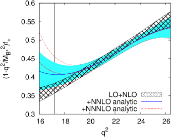
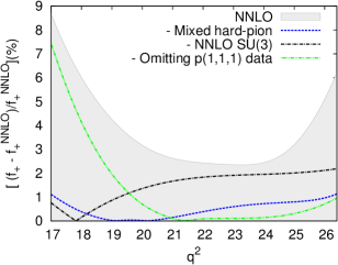
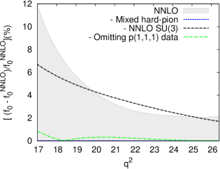
First, we study the effects of truncating the chiral expansion by adding next-to-NNLO (NNNLO) analytic terms in our fits with coefficients constrained with the same priors as the NNLO coefficients. The variations in due to changing the order of the PT analytic terms are shown in Fig. 13. The fits of different orders are consistent in the region where most of the simulation data are located. Although the central values and errors differ noticeably between the NLO and NNLO fits, the central values and errors of the NNNLO fit are very close to the NNLO fit, indicating that the chiral extrapolation has stabilized by NNLO. As discussed earlier, the NLO coefficients are well determined by the data and we use well-motivated priors based on expectations from PT for the NNLO and higher order terms. The fact that the error saturates with NNLO shows that the preferred fit already incorporates the uncertainty from truncating the chiral expansion, and that we do not need to add an additional systematic error. The NNLO fit error as a function of is shown in Fig. 14.
The standard soft-pion HMrSPT fits of have reasonable confidence levels, but those of do not. Here we estimate the effect of using the hard-pion formalism by using standard HMrSPT for but still employing hard-pion PT for . The resulting difference from the preferred fit is small, less than 1% for . The same conclusion also holds for the form factor .
We use SU(2) PT, instead of SU(3) PT, for our central fit. To estimate the effect of this choice, we restore the strange-quark dependence of the logarithm and analytic terms in Eq. (32). A practical issue arises with NNLO SU(3) PT, where the terms proportional to the sea-quark mass, , are not well constrained by our data because the strange sea-quark mass is so similar on all of our ensembles. To obtain some sensitivity to , we include data on an additional fm ensemble with an unphysically small strange-quark mass, . With the inclusion of this ensemble, we find the fit parameters for the terms involving are better constrained. The differences between the NNLO SU(3) fits and the preferred fits are shown in Fig. 14. For , the difference is within the statistical error. For , the difference lies outside the statistical error for some of the simulated range, but the NNLO SU(3) fit quality is poor, with a p-value of 0.01. Because SU(3) PT does not provide a good description of our data for , we do not take the difference between NNLO SU(2) and SU(3) fits as a systematic error.
To check how our results are affected by data with high momenta, we also perform a fit excluding data with . As shown in Fig. 14, the form factors and from the low-momentum fit agree very well with those from the preferred full-data fit for the region . The systematic difference increases for small , where the highest-momentum data provide important information.
Figure 14 summarizes the effects of all these variations. Comparing the deviations between the central values of the alternate and preferred fits to the statistical error of the preferred fit, we find that the deviations are almost always smaller than the statistical error of our preferred fit. This confirms that fit errors of our preferred fits adequately account for the systematic effects associated with these variations. We therefore do not quote any additional systematic error due to these sources.
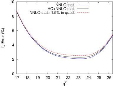
We include heavy-quark discretization effects in our chiral-continuum extrapolation. As a consistency check, we compare our result with a power counting estimate obtained by evaluating in Eq. (46) at the fm lattice spacing, setting the coefficients and taking MeV for the heavy-quark scale. We find %. Figure 15 shows that the NNLO fit error (without the heavy-quark discretization effects) added to the 1.5% power-counting estimate in quadrature yields a similar error to that of the full fit. Thus, again, it is not necessary to add an additional error to that of the preferred chiral-continuum fit.
IV.2 Light- and bottom-quark mass uncertainties
The effect of mistuning the -quark mass in our simulation has been largely reduced via the corrections described in Sec. II.6. Errors still arise, however, from the uncertainty in the tuned value itself and from the procedure for shifting the form factors. From Eq. (31) we estimate the relative error by
| (48) |
where is related to the uncertainty due to the error in while is the uncertainty on the normalized slope. The values of the physical with errors are given in Table 7, and we can find the statistical uncertainty of the normalized slope using Table 8. Using Eq. (31), we find that the value of on all ensembles is at most 0.6%. We take the average value for on all ensembles, which is 0.4%, to be the error due to tuning , and assign the same error to and .
To obtain the physical form factors, we evaluate the result of the chiral-continuum fit at the physical light- and strange-quark masses determined from the MILC Collaboration’s analysis of light pseudoscalar mesons 0903.3598 . (Although we use SU(2) PT, we include an analytic term proportional to to allow for a slight shift to the physical strange sea-quark mass.) The errors on the physical and are 3.5% and 3.0%, respectively. We vary the light- and strange-quark masses at which the chiral-continuum fit function is evaluated by plus and minus one standard deviation, and find that it produces differences below 0.4% in both form factors.
IV.3 Lattice scale
We convert the lattice form factors and pion energies to physical units using the relative scale determined from the static-quark potential (see Table 3) and the absolute scale fm 1112.3051 . The statistical uncertainties on are negligible. We propagate the uncertainty in by shifting it and repeating the chiral-continuum fit. We find shifts of at most in the range of simulated momenta.
IV.4 Current renormalization
With the mostly nonperturbative renormalization procedure that we use for the heavy-light currents, there are two sources of error. The first is due to the nonperturbatively calculated flavor diagonal factors and . Their values and errors are given in Table 6. We estimate the systematic error due to the uncertainties of and by varying their values by one sigma and looking for the maximum deviations in the form factors and . The resulting deviations are small, ranging from 0.4% to 0.6%.
The second source of error is due to the truncation of the perturbative expansion in the calculation of the . Because the are defined from ratios of renormalization constants, their perturbative corrections are small by construction. Indeed, as seen in Table 6, for they are less than 1% and for they range between 2–3%. For the scale-independent vector current, we observe that the one-loop corrections to are smaller than those for , and we use the same error estimate for both. In order to accommodate possible accidental cancellations, we take the error as , where is an upper bound of the one-loop correction to in the range of heavy-quark mass that corresponds to the range of lattice spacings included in our analysis. The coupling is evaluated at the scale of the next-to-finest lattice spacing in our calculation, fm. This procedure yields an error estimate of 1%, which is larger than the one-loop correction to over most of the mass range, and amounts to about 50% of the one-loop correction to in the mass range that corresponds to the three finest lattice spacings. This leads to an error of 1% for both and due to the perturbative renormalization factors.
IV.5 Finite volume effects
We estimate the size of the finite-volume effects by replacing the infinite-volume chiral logarithms with discrete sums and repeating the chiral-continuum extrapolation. The change in our preferred fit after including finite-volume corrections is very small, less than 0.01%, which we simply neglect.
IV.6 Summary
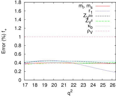
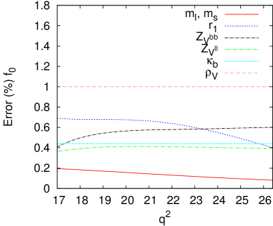
Figures 16 and 17 visually summarize the systematic error budget for the vector and scalar form factors in the simulated lattice-QCD momentum range. By far the largest contribution to the total uncertainty is from the fit error, which includes the statistical uncertainty in addition to the chiral-continuum extrapolation and heavy-quark discretization errors. The total error on is smallest, about 3%, in the region of – GeV2.
The subdominant errors, such as those from heavy-quark mass tuning, the current renormalization etc., have mild dependence, as can be seen in Fig. 16. We therefore treat them as constant in when propagating them. For each source, we take the maximum estimated error in the simulated range; we then add these individual error estimates in quadrature to obtain an overall additional systematic error . We find and .
In the next section, we will use our result for to obtain via a combined fit with experimental data to the expansion. Due to phase-space suppression, the experiments have poor access to the large- region. On the other hand, the lattice-QCD form factor has a larger error than experiment at small due to the sizable extrapolation. As discussed below, the value of is mostly determined in the region , which is at the low end of the range where the lattice-QCD form-factor error is still small. We therefore provide tabulated error budgets for the two form factors from our calculation at the particular kinematic point in Table 10. The error on is approximately 3.4%, which is about one third of the error on our previously-determined form factor in Ref. 0811.3640 .
| Uncertainty | ||
|---|---|---|
| Statistical+PT+HQ+ | 3.1 | 3.8 |
| Scale | 0.5 | 0.7 |
| Non-perturbative | 0.4 | 0.6 |
| Non-perturbative | 0.4 | 0.4 |
| Perturbative | 1.0 | 1.0 |
| Heavy-quark mass mistuning | 0.4 | 0.4 |
| Light-quark mass tuning | 0.4 | 0.2 |
| Total | 3.4 | 4.1 |
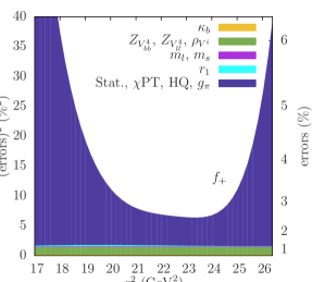
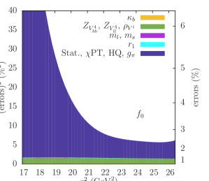
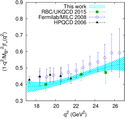
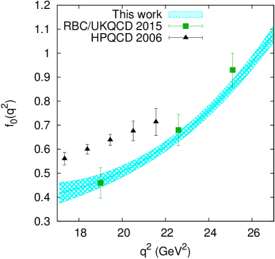
We compare our results for and with full errors, which are obtained by adding the fit errors from the PT fits and in quadrature, with previous lattice-QCD calculations in Fig. 18. Our result for agrees with previous results obtained at GeV2 from Refs. hep-lat/0601021 ; 0811.3640 ; Flynn:2015mha , but is more precise. Our result for is consistent with Ref. Flynn:2015mha , but not with Ref. hep-lat/0601021 .
V expansion and determination of
The chiral-continuum extrapolation described in the previous sections yields the form factors in the range . In this section, we extrapolate them to the full kinematic range using the model-independent expansion. The form factors resulting from the chiral-continuum extrapolation are functions specified by a set of parameters. One could, in principle, incorporate the expansion with the PT expansion from the outset (see, e.g., Ref. 1206.4936 ). With such an approach, however, the coefficients of the expansion will have a nontrivial dependence on and that must be derived from the underlying chiral effective theory. Because the dependence of the coefficients on and is unknown, we instead carry out the extrapolation in two steps, taking the chiral-continuum extrapolated results and feeding them into the expansion. We introduce a functional method to perform the expansion. We also apply the expansion to the experimental data and, after verifying that the fits to experiment and to lattice QCD are consistent, we carry out a combined fit to obtain . A byproduct of the last step is a precise determination for constrained by lattice QCD at high and experiment at low .
V.1 expansions of heavy-light semileptonic form factors
The expansion involves mapping the variable to a new variable by hep-ph/9702300
| (49) |
where and is chosen for convenience below. This change of variables maps the whole complex plane onto the unit disk in the plane, where the upper (lower) path along the branch cut is mapped to the lower (upper) half of the circle enclosing the unit disk in the complex plane. Choosing centers the full kinematic range for semileptonic decay around the origin , and, moreover, restricts to . The small, bounded interval, together with a constraint from unitarity ensures convergence of the expansion. As discussed below, we find in practice that the convergence is rapid.
The form factors and are analytic in except for the branch cut and poles in . We can write
| (50) |
where , , are the Blaschke factors, which are introduced to remove the poles of in the region , and are the outer functions hep-ph/9702300 ; hep-ph/9412324 . We choose simple outer functions and employ the following formulas to expand the form factors
| (51) | |||||
| (52) |
Equation (51) is known as the Bourrely-Caprini-Lellouch (BCL) expansion 0807.2722 , which is constructed to reproduce the threshold behavior at and the asymptotic behavior as . Equation (52) is a simple series expansion of in .
The BCL coefficients in Eq. (51) and (52) obey the unitarity constraint 0807.2722 ; hep-ph/9702300
| (53) |
where the element satisfies and depends on the choice of 0807.2722 . We tabulate the values of for the form factors in Table 11. The inequality saturates when . Although we do not incorporate this constraint into our fits, we check that our results satisfy it.
| 0.1032 | 0.0408 | 0.0357 | 0.0394 | 0.0195 | 0.0055 | 0.0004 | |
| 0.0198 | 0.0042 | 0.0109 | 0.0059 | 0.0002 | 0.0012 | 0.0011 |
V.2 Functional method for the expansion
In previous work, we have used synthetic data points generated from the PT fit as inputs to the fit 0811.3640 , but here we take a new approach. We exploit the facts that the PT expansion is linear in the fit parameters and that it contains only a finite number of independent functions (see Eq. (32)). We construct a covariance function , defined as the covariance of any pair of points (), using the set of functionals from the PT expansion. Our new approach is to formulate the expansion using the eigenfunctions of an integral operator defined from .
Let us start with the NLO PT expression Eq. (32), as an example. Because and are linear in their coefficients and , we can express them both in the compact form
| (54) |
where
| (56) | |||||
| (58) |
and where and the variables are defined in Eqs. (35)–(37). Any linear combination of and can be written as
| (62) | |||||
| (66) |
with functions of . The uncertainty of the function is encoded in the uncertainty in the coefficient vector . In all these expressions, we are only interested in the terms with (or ) dependence and, hence, dependence. We can now define the covariance function in some valid domain . Explicitly,
| (67) |
where
| (70) |
and Cov is the covariance matrix of the involved coefficients
| (71) |
The covariance function is a Mercer kernel mercer , and Mercer’s theorem ensures that there exists a set of orthonormal functions defined over the domain such that
| (72) |
where , are the eigenvalues and eigenfunctions of the operator induced by the integral equation,
| (73) |
The form factor can naturally be expanded in the basis of : we only need to project the expansions in Eqs. (51) and (52) onto the same basis. The process of finding the expansion coefficients is equivalent to minimizing the following function (in analogy to the usual function, replacing the sum over discrete points with an integral over a continuous variable):
| (74) | |||||
where
| (75) |
is the form factor function from the PT fit expanded in terms of , and
| (76) |
are functions rewritten from the functions defined in Eqs. (51) and (52). For brevity we define
| (77) | |||||
| (78) |
To summarize, we expand any form factor function obtained from the chiral-continuum extrapolation in the basis formed by the eigenfunctions of its covariance function . We then project the expansion onto the same basis. Finally, we solve for the expansion parameters by minimizing the function defined in Eq. (74).
V.3 Details on expansion of the form factors
In addition to the fit errors from the chiral-continuum fit, we also need to propagate the subdominant errors, which have very mild dependence. We treat them as constant in and add them in quadrature, obtaining and . To include this effective subdominant error to the fit, we slightly modify the covariance function defined in Eq. (67) by
| (79) |
where the new covariance matrix includes the subdominant error,
| (80) |
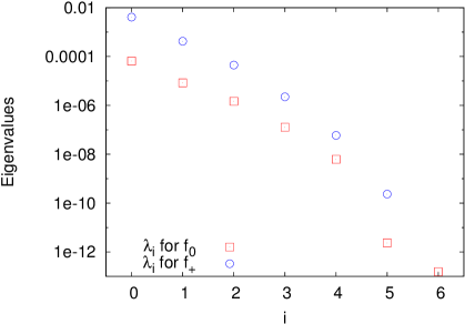
In the function array defined in Eq. (70), only a relatively small number of the elements are independent functions. For example, there are 42 terms in the NNLO SU(2) PT fit functions for (including the HQ discretization contributions). Many of them, however, are set to zero in the continuum limit or become constant once the light-quark mass is fixed at its physical value. In the end, the chiral-continuum extrapolated is described by only 6 independent functions. For , the number of independent functions is 7. Although we work in the functional basis in which the covariance function is diagonalized, singular modes can arise because is built upon , which itself may have singular modes. Figure 19 shows the spectra of the operator for form factor . The spectrum of contains two very small eigenvalues , and they are well separated from the other modes. When we discard these two modes, the fit quality of the functional fit improves from to . For , we do not need to apply any cut on the eigenvalues.
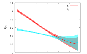
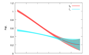
We first consider separate fits of and without any constraints on the coefficients of the expansion. With , or three free parameters , we obtain a low confidence level, , for the fit to . The analogous three-parameter fit for results in an acceptable confidence level, . With we find good confidence levels for both form factors as well as sizable changes in the central values and errors (compared to the case). The results of unconstrained fits of and with several values of for and are given for comparison in Table 12. The kinematic constraint is satisfied automatically, as is shown in Fig. 20 (left).
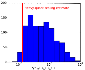
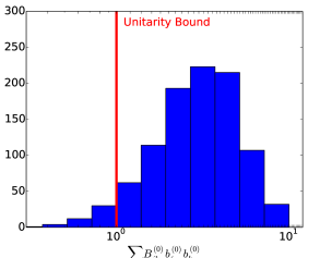
The -expansion coefficients should approximately satisfy the unitarity bound Eq. (53). Figure 21 (right) shows the bootstrap-sample distribution of from the fits for . The unitarity condition is marginally satisfied. In the case of , the sum is much smaller than the unitarity bound. Reference hep-ph/0509090 pointed out that the smallness is expected based on heavy-quark physics. The value of should be of order , which is about 0.013 with a conservative choice of GeV. The bootstrap-sample distribution of from the fits for is shown against the heavy-quark estimate in Fig. 21 (left). They are consistent with each other.
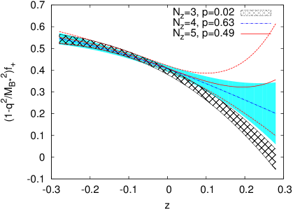
The result of the fits of with the kinematic constraint are shown in Fig. 20 (right). With this constraint, we again examine how the fit varies with higher order . We find that the fit central values do not change significantly when we change from 4 to 5, in contrast to the case from 3 to 4, as is shown in Fig. 22 and Table 13.
| /dof | 1.1 | 1.0 | 1.6 | 3.1 | 0.54 |
|---|---|---|---|---|---|
| dof | 3 | 2 | 1 | 2 | 1 |
| 0.27 | 0.33 | 0.2 | 0.05 | 0.46 | |
| 0.052(16) | 0.024(39) | 2(4) | 0.60(24) | 2.0(11) | |
| 0.12(6) | 0.23(20) | 0.40(34) | 0.14(9) | 0.20(17) | |
| 0.409(16) | 0.409(12) | 0.407(15) | 0.493(22) | 0.510(23) | |
| 0.72(13) | 0.63(20) | 0.60(22) | 2.1(2) | 1.7(2) | |
| 1.0(2) | 0.3(1.3) | 0.3(1.7) | 0.8(5) | 1.2(9) | |
| 1(2) | 4(5) | 3(1) | |||
| 7(7) | |||||
| Fit | |||
|---|---|---|---|
| /dof | 2.5 | 0.64 | 0.73 |
| dof | 6 | 4 | 2 |
| 0.02 | 0.63 | 0.48 | |
| 0.11(2) | 0.016(5) | 1.0(2.3) | |
| 0.33(8) | 2.8(1.7) | 8(19) | |
| 0.00(4) | 0.20(14) | 0.36(27) | |
| 0.395(15) | 0.407(15) | 0.408(15) | |
| 0.93(11) | 0.65(16) | 0.60(21) | |
| 1.6(1) | 0.5(9) | 0.2(1.4) | |
| 0.4(1.3) | 3(4) | ||
| 5(5) | |||
| 0.515(19) | 0.507(22) | 0.511(24) | |
| 1.84(10) | 1.77(18) | 1.69(22) | |
| 0.14(25) | 1.3(8) | 2(1) | |
| 4(1) | 7(5) | ||
| 3(9) |
| 0.407(15) | 0.65(16) | 0.46(88) | 0.4(1.3) | 0.507(22) | 1.77(18) | 1.27(81) | 4.2(1.4) | |
| 1 | 0.451 | 0.161 | 0.102 | 0.331 | 0.346 | 0.292 | 0.216 | |
| 1 | 0.757 | 0.665 | 0.430 | 0.817 | 0.854 | 0.699 | ||
| 1 | 0.988 | 0.482 | 0.847 | 0.951 | 0.795 | |||
| 1 | 0.484 | 0.833 | 0.913 | 0.714 | ||||
| 1 | 0.447 | 0.359 | 0.189 | |||||
| 1 | 0.827 | 0.500 | ||||||
| 1 | 0.838 | |||||||
| 1 |
We perform several additional checks to confirm the stability of our results against various fit choices. In our preferred fit, we set the integral range in Eq. (74) to be (or equivalently ). The results, however, do not change noticeably if we extend the integral range to which covers the full range of simulated lattice momenta. This is because the statistical fluctuations and correlations of the form-factor functions are largely decided by the region , where the PT fit results are the most precise.
We also try removing the smallest eigenvalue from the covariance function for ; we find that the resulting central values are essentially unaffected. Finally, we also try the fit using, instead of the BCL formula, the Boyd-Grinstein-Lebed (BGL) formula, which uses more complicated outer functions hep-ph/9412324 . We find that the resulting form factors are within one standard deviation of the BCL result.
To summarize, we obtain our preferred result from a simultaneous fit to and with and with imposing the kinematic constraint . The results for the two form factors and are plotted in Fig. 23. In this plot, the form factors obtained from the PT fit are overlaid on the results of the fit. The fit faithfully reproduces the PT fits in the region where PT is reliable (indicated by the ranges of the hatched bands). The coefficients with errors from our preferred fit and their correlation matrix are provided in Table 14. This information is sufficient to reproduce the lattice form-factor results over the full kinematic range.
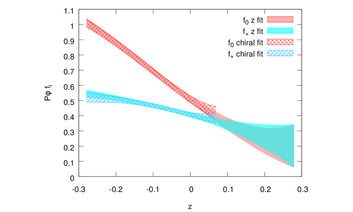
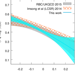
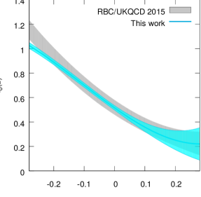
Figure 24 shows a comparison of our results with other theoretical calculations of the form factors Imsong:2014oqa ; Flynn:2015mha . While our results are consistent with the previous results, ours are significantly more precise in the region of .
Finally, it is interesting to compare the lattice form factors with theoretical expectations from heavy-quark symmetry. In the soft-pion limit, the vector and scalar form factors and are related as Burdman:1993es
| (81) |
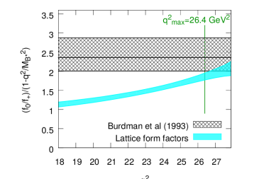
up to corrections of . This expression updates the leading-order result of Ref. Wise:1992hn to include the correction, which turns out to be simply the additional multiplicative factor in the soft-pion limit. In Fig. 25 we plot the ratio of obtained using the coefficients of our preferred -expansion in Table 14. We also show the theoretical expectation from Eq. (81), taking the HPQCD Collaboration’s recent three-flavor lattice-QCD result for the decay-constant ratio Colquhoun:2015oha , and using the same value of as in our chiral-continuum extrapolation. The large width of the expected band is due to the generous range taken for . Higher-order corrections in the heavy-quark expansion are expected to be small. Taking a conservative value for MeV and GeV, one would estimate corrections to be about 1%. The difference of from one also provides a measure of , which would indicate that corrections may even be below the percent level. The lattice form factors agree with the theoretical expectation for .
V.4 Determination of
We now combine our lattice form factors with experimental data for to obtain . The Standard-Model partial branching fraction is , where is defined in Eq. (1). The contribution from is negligible due to the small lepton mass. Given , the branching fraction in the th bin is
| (82) |
where is a constant. For the combined lattice plus experiment fit, we define a for the experimental measurements as
| (83) |
where is the experimentally-measured branching fraction in the th bin ( is a shorthand notation for each bin in each experiment included in the fit) and is the experimental covariance matrix, including the statistical and all systematic errors.
We use the experimental results compiled by the Heavy Flavor Averaging Group (HFAG) 1207.1158 : BaBar untagged 6-bin analysis (2011) 1005.3288 , Belle untagged 13-bin analysis (2011) 1012.0090 , BaBar untagged 12-bin analysis (2012) 1208.1253 and Belle tagged analysis with 13 bins for the and 7 bins for the mode (2013) 1306.2781 . For convenience in the fit, we assume isospin symmetry to convert the Belle tagged data to the mode via
| (84) |
where ps and are from the PDG PDG2014 .
We omit systematic correlations between the BaBar and Belle analyses, because they do not share any major systematic errors. The BaBar 6-bin and 12-bin data have very small overlaps in the selection of samples, so the statistical errors can be considered approximately uncorrelated. There is some systematic correlation between the two analyses, which is, however, supposed to be insignificant JDingfelder . The Belle untagged and tagged data are also largely uncorrelated because the dominant source of systematic errors in these two measurements are very different. In summary, we take the four experimental analyses as independent measurements.
On the other hand, there are systematic correlations between the two isospin modes of the Belle tagged data, which we estimate as follows. Let and be the branching fractions in the th and th bin of the charged and neutral decay modes, respectively. Let be the systematic uncertainties of the two modes from source and be the correlation between them. Then we estimate the off-block-diagonal elements of the systematic error covariance matrix by
| (85) |
where the sum is over all sources of systematic errors. That said, only a few of the systematic errors contribute noticeably to the sum and the biggest source of error, the tag calibration, dominates. From the correlation matrices, we construct the total covariance matrices of each isospin decay mode by adding the statistical matrices and the systematic matrices. We then take the direct sum of the covariance matrices of the and modes block-diagonally and add the off-block-diagonal elements so that we can fit them simultaneously.
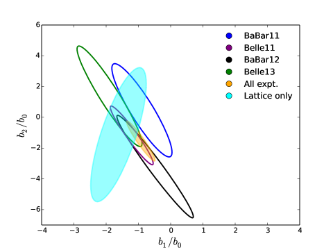
We first fit the expansion to the experimental data only and without any constraints on the coefficients. We use the BCL formula with three parameters, , where the normalization is . The result is shown in Table 15. To check the consistency in the shape among the experimental data sets, we also fit each experimental data set separately. The individual fits all have acceptable confidence levels and values, but the combination of all four data sets gives a rather poor fit that is not improved by going to higher order in , , . The poor fit stems from the BaBar11 measurement, which is only marginally consistent with the other three. Figure 26 compares the shapes (slopes and curvatures ) of the separate and combined experimental fits with the lattice-only fit. The lattice form factor shape is consistent with all of the experimental results.
| Fit | /dof | dof | ||||
|---|---|---|---|---|---|---|
| All exp. | 1.5 | 48 | 0.02 | 0.93(22) | 1.54(65) | 1.53(4) |
| BaBar11 1005.3288 | 2 | 3 | 0.12 | 0.89(47) | 0.5(1.5) | 1.36(7) |
| BaBar12 1208.1253 | 1.2 | 9 | 0.31 | 0.48(59) | 3.2(1.7) | 1.54(9) |
| Belle11 1012.0090 | 1.1 | 10 | 0.36 | 1.21(33) | 1.18(95) | 1.63(7) |
| Belle13 1306.2781 | 1.2 | 17 | 0.23 | 1.89(50) | 1.4(1.6) | 1.56(8) |
To perform a combined fit to the lattice and experimental data, we define the total chi squared function,
| (86) |
where the lattice and experimental chi squared functions are defined in Eqs. (74) and (83), respectively. The fit is performed to these five independent data sets with common shape parameters and overall normalization by minimizing Eq. (86). Table 16 summarizes the various fit results. Due to the tension between the experimental data sets, the value of the fit to the lattice result and all experiments is only 0.02. Table 17 shows the contributions to the total from each data set of the combined fit. By far the largest contribution to is from the BaBar 6-bin data set, similar to what we find for the experiment-only fits presented in Table 15.
In the combined fit to lattice form factors and experimental data, the kinematic constraint between and at is unimportant for the determination of . This is because the experimental data constrain the shape at low . Removing the kinematic constraint from the combined fit and fitting only with the vector form factor changes neither the coefficients of the expansion nor the value of . We also try varying the number of parameters in the expansion (). The results are shown in Table 18. Compared to our preferred fit with , the fit using gives a very low value and a shift of about in both the form factor and , while the fit result using nearly coincides with that of the fit and the values of are almost identical.
| Fit | /dof | dof | value | () | ||||
|---|---|---|---|---|---|---|---|---|
| Lattice+exp.(all) | 1.4 | 54 | 0.02 | 0.419(13) | 0.495(55) | 0.43(14) | 0.22(31) | 3.72(16) |
| Lattice+BaBar11 1005.3288 | 1.1 | 9 | 0.38 | 0.414(14) | 0.488(73) | 0.24(22) | 1.33(44) | 3.36(21) |
| Lattice+BaBar12 1208.1253 | 1.1 | 15 | 0.34 | 0.415(14) | 0.551(72) | 0.45(18) | 0.27(41) | 3.97(22) |
| Lattice+Belle11 1012.0090 | 0.9 | 16 | 0.55 | 0.412(13) | 0.574(65) | 0.40(16) | 0.38(36) | 4.03(21) |
| Lattice+Belle13 1306.2781 | 1.0 | 23 | 0.42 | 0.406(14) | 0.623(73) | 0.13(22) | 0.92(45) | 3.81(25) |
| data set | # data | /# data | |
|---|---|---|---|
| Lattice | 11 | 4.8 | 0.44 |
| BaBar11 1005.3288 | 6 | 20.9 | 3.5 |
| BaBar12 1208.1253 | 12 | 15.1 | 1.3 |
| Belle11 1012.0090 | 13 | 13.8 | 1.1 |
| Belle13 1306.2781 | 20 | 23.5 | 1.2 |
| Total | 62 | 78.2 | 1.26 |
| /dof | dof | value | |||||||
|---|---|---|---|---|---|---|---|---|---|
| 2.5 | 56 | 0.0 | 0.425(12) | 0.424(31) | 0.59(9) | 3.63(11) | |||
| 1.4 | 54 | 0.02 | 0.419(13) | 0.495(55) | 0.43(14) | 0.22(31) | 3.72(16) | ||
| 1.5 | 52 | 0.01 | 0.418(13) | 0.491(56) | 0.31(30) | 0.01(55) | 0.6(1.9) | 3.72(16) |
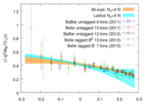
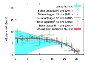
The experimental data are plotted in Fig. 27 (left) along with the fits to the lattice data and to all experimental data. The lattice form factor and experimental measurements provide complementary information and, when combined, yield an accurate description of the form factor over the full- range and hence a precise determination of . The plot shows that the experimental data dominate the determination of the form-factor shape in the large- (small-) region while the lattice-QCD form factor dominates the small- (large-) region. In the intermediate region around (), the lattice-QCD and experimental uncertainties are similar in size. This region is decisive in determining and, hence, can be used to estimate the separate contributions from lattice and experimental data to the uncertainty. At , the error on the lattice-QCD form factor is about 3.4% (see Table 10) and the error on from the experiment-only fit is 2.8% at the same momentum. Adding these two errors in quadrature gives a total uncertainty of , which is consistent with the error on obtained from the full fit, . Another estimate of the individual error contribution to can be obtained from the uncertainty on the fit parameters from the separate lattice-QCD and experiment fits. From the fit to all experimental data in Table 15, the normalization is . Similarly, the lattice-only fit gives the normalization . Assuming no correlation, one would obtain , which is close to what we obtain from the combined fit.
VI Results and conclusion
Our final result for , obtained from our preferred fit combining our lattice-QCD calculation of the form factor with experimental measurements of the corresponding decay rate, is
| (87) |
The error includes all experimental and lattice-QCD uncertainties. The contribution from lattice QCD to the total error is now comparable to that from experiment. The error reported here, following HFAG 1207.1158 , does not apply the PDG prescription for discrepant data; that prescription PDG2014 would scale the error by a factor of . As can be seen from Table 17 and Fig. 26, the low fit quality is due to the tension between the BaBar11 data set and the others. An inspection of all the experimental data in Fig. 27 shows that the point near in the BaBar11 data set is lower than the others and a bit more precise than one might have anticipated, but does not suggest that this or any of the data sets have any systematic problems.
We compare our determination of with other results in Fig. 28. In particular, our result is consistent with the recent determination from HFAG using our collaboration’s 2008 form-factor determination 0811.3640 obtained from a small subset of the gauge-field ensembles used in this work. The difference in the central values is due to a small shift in the central values for the form factor of this analysis compared to our previous analysis 0811.3640 . As shown in Fig. 18 (left), the form factor from this analysis is consistent within errors with the previous analysis, but shifted slightly downward and with an error smaller by roughly a factor of three. The two analyses have very little statistical and systematic correlation. Our result is also compatible with Standard-Model expectations from CKM unitarity Laiho:2009eu ; Bona:2006ah . Although our determination of is higher than that in Ref. 0811.3640 , and thus closer to the determination from inclusive semileptonic decays 1207.1158 , the inclusive-exclusive disagreement is still greater than 2.
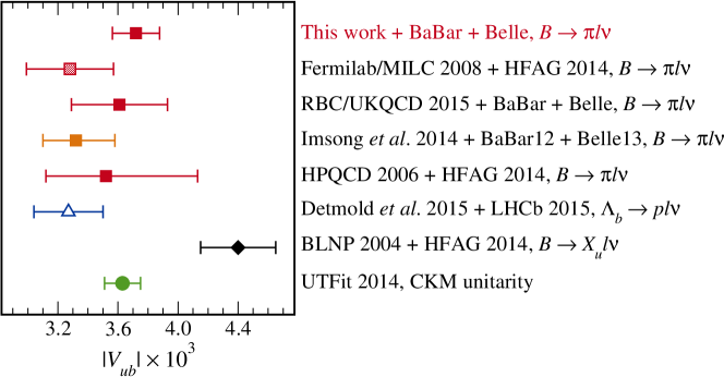
A byproduct of the combined lattice and experiment fit is a more precise determination of the vector and scalar form factors than from the lattice-QCD calculation alone. Both form factors and are well determined from lattice QCD in the high region, and is strongly constrained by experiment in the low region. This information is then transferred to via the kinematic constraint . The resulting form factors are shown in Fig. 29. The corresponding -expansion coefficients and their correlations are given in Table 19. These represent the present best knowledge of the form factors, and can be used in other phenomenological applications or to test other nonperturbative QCD calculations.
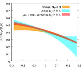
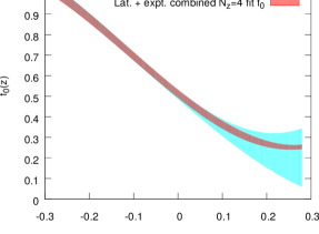
Future improvements in the determination of the semileptonic form factor will further reduce the uncertainty on . If the uncertainty of at GeV2 can be reduced further from % to %, we would expect a precision of 3% in , using the current experimental input. With the anticipated improvement in the experimental rate measurement from Belle II, this error would be reduced further. The reduction of uncertainty in is expected with the newly-available MILC gauge ensembles that are being generated using the highly improved staggered quark (HISQ) action Bazavov:2012xda . The new HISQ ensembles have statistics similar to the asqtad ensembles, but with much smaller light-quark discretization effects. Further, the HISQ ensembles simulated at the physical light-quark masses will remove the need for a chiral extrapolation, thereby eliminating a significant source of uncertainty in this work. These ensembles have already helped to determine the form factor Bazavov:2013maa and the leptonic decay constants and Bazavov:2014wgs , and hence the relevant CKM matrix elements , and , with high precision. All of these improvements will further refine and reduce the uncertainties in , and may also help to resolve the inclusive/exclusive puzzle.
Acknowledgements.
We thank Jochen Dingfelder for the helpful information about the experimental measurements and HFAG averaging procedure. D.D. thanks Peter Lepage for sharing his lsqfit code (github.com/gplepage/lsqfit) which is extensively used in the fitting procedures of the analysis. We also thank Heechang Na for valuable discussions. Computations for this work were carried out with resources provided by the USQCD Collaboration, the Argonne Leadership Computing Facility, the National Energy Research Scientic Computing Center, and the Los Alamos National Laboratory, which are funded by the Office of Science of the United States Department of Energy; and with resources provided by the National Institute for Computational Science, the Pittsburgh Supercomputer Center, the San Diego Supercomputer Center, and the Texas Advanced Computing Center, which are funded through the National Science Foundation’s Teragrid/XSEDE Program. This work was supported in part by the U.S. Department of Energy under Grants No. DE- FG02-91ER40628 (C.B., J.K.), No. DE-FC02-12ER41879 (C.D., J.F., L.L.), No. DE-SC0010120 (S.G.), No. DE-FG02-91ER40661 (S.G., R.Z.), No. DE-FC02-06ER41443 (R.Z.), No. DE-FG02-13ER42001 (D.D., A.X.K.), No. DE-FG02-13ER41976 (D.T.), No. DE-SC0010114 (Y.M.); by the National Science Foundation under Grants No. PHY-1067881, No. PHY-10034278 (C.D., L.L., S-W.Q.), No. PHY-1417805 (J.L., D.D.), No. PHY-1212389 (R.Z.), No. PHY-1316748 (R.S.); by the URA Visiting Scholars’ program (C.M.B., D.D., A.X.K., Y.L.); by the MINECO (Spain) under Grants FPA2010-16696, FPA2006-05294, and Ramón y Cajal program (E.G.); by the Junta de Andalucía (Spain) under Grants FQM-101 and FQM-6552 (E.G.); by European Commission hunder Grant No. PCIG10-GA-2011-303781 (E.G.); by the German Excellence Initiative and the European Union Seventh Framework Programme under grant agreement No. 291763 as well as the European Union’s Marie Curie COFUND program (A.S.K.); and by the Basic Science Research Program of the National Research Foundation of Korea (NRF) funded by the Ministry of Education (No. 2014027937) and the Creative Research Initiatives Program (No. 2014001852) of the NRF grant funded by the Korean government (MEST) (J.A.B.). This manuscript has been co-authored by an employee of Brookhaven Science Associates, LLC, under Contract No. DE-AC02-98CH10886 with the U.S. Department of Energy. Fermilab is operated by Fermi Research Alliance, LLC, under Contract No. DE-AC02-07CH11359 with the U.S. Department of Energy.| 3.72(16) | 0.419(13) | 0.495(54) | 0.43(13) | 0.22(31) | 0.510(19) | 1.700(82) | 1.53(19) | 4.52(83) | |
| 1 | 0.870 | 0.400 | 0.453 | 0.428 | 0.175 | 0.201 | 0.119 | 0.009 | |
| 1 | 0.140 | 0.455 | 0.342 | 0.224 | 0.174 | 0.047 | 0.033 | ||
| 1 | 0.789 | 0.874 | 0.068 | 0.142 | 0.025 | 0.007 | |||
| 1 | 0.879 | 0.051 | 0.253 | 0.098 | 0.234 | ||||
| 1 | 0.076 | 0.038 | 0.018 | 0.200 | |||||
| 1 | 0.043 | 0.604 | 0.388 | ||||||
| 1 | 0.408 | 0.758 | |||||||
| 1 | 0.457 | ||||||||
| 1 |
References
- [1] N. Cabibbo, Phys. Rev. Lett. 10, 531 (1963).
- [2] M. Kobayashi and T. Maskawa, Prog. Theor. Phys. 49, 652 (1973).
- [3] A. Crivellin and S. Pokorski, Phys. Rev. Lett. 114, 011802 (2015) [arXiv:1407.1320 [hep-ph]].
- [4] E. Dalgic, A. Gray, M. Wingate, C. T. H. Davies, G. P. Lepage and J. Shigemitsu [HPQCD Collaboration], Phys. Rev. D 73, 074502 (2006) [Erratum-ibid. D 75, 119906 (2007)] [hep-lat/0601021].
- [5] J. A. Bailey et al. [Fermilab Lattice and MILC Collaborations], Phys. Rev. D 79, 054507 (2009) [arXiv:0811.3640 [hep-lat]].
- [6] Y. Amhis et al. [Heavy Flavor Averaging Group Collaboration], arXiv:1207.1158 [hep-ex]; updated results as of Summer 2014 on the website http://www.slac.stanford.edu/xorg/hfag/
- [7] P. del Amo Sanchez et al. [BaBar Collaboration], Phys. Rev. D 83, 032007 (2011) [arXiv:1005.3288 [hep-ex]].
- [8] J. P. Lees et al. [BaBar Collaboration], Phys. Rev. D 86, 092004 (2012) [arXiv:1208.1253 [hep-ex]].
- [9] H. Ha et al. [BELLE Collaboration], Phys. Rev. D 83, 071101 (2011) [arXiv:1012.0090 [hep-ex]].
- [10] A. Sibidanov et al. [Belle Collaboration], Phys. Rev. D 88, 032005 (2013) [arXiv:1306.2781 [hep-ex]].
- [11] V. G. Lüth, arXiv:1209.4674 [hep-ex].
- [12] F. Bahr et al. [ALPHA Collaboration], PoS ICHEP 2012, 424 (2013) [arXiv:1211.6327 [hep-lat]].
- [13] J. M. Flynn, T. Izubuchi, T. Kawanai, C. Lehner, A. Soni, R. S. Van de Water and O. Witzel, [arXiv:1501.05373 [hep-lat]].
- [14] C. M. Bouchard, G. P. Lepage, C. J. Monahan, H. Na and J. Shigemitsu [HPQCD Collaboration], PoS LATTICE 2013, 387 (2014) [arXiv:1310.3207 [hep-lat]].
- [15] S. W. Bosch, B. O. Lange, M. Neubert and G. Paz, Phys. Rev. Lett. 93, 221801 (2004) [hep-ph/0403223].
- [16] D. Du, J. A. Bailey, A. Bazavov, C. Bernard, A. X. El-Khadra, S. Gottlieb, R. D. Jain and A. S. Kronfeld et al., PoS LATTICE 2013, 383 (2014) [arXiv:1311.6552 [hep-lat]].
- [17] J. A. Bailey et al. [Fermilab Lattice and MILC Collaborations], arXiv:1411.6038 [hep-lat].
- [18] A. X. El-Khadra, A. S. Kronfeld, P. B. Mackenzie, S. M. Ryan and J. N. Simone, Phys. Rev. D 64, 014502 (2001) [hep-ph/0101023].
- [19] A. Bazavov et al., Rev. Mod. Phys. 82, 1349 (2010) [arXiv:0903.3598 [hep-lat]].
- [20] C. W. Bernard, T. Burch, K. Orginos, D. Toussaint, T. A. DeGrand, C. E. Detar, S. Datta and S. A. Gottlieb et al., Phys. Rev. D 64, 054506 (2001) [hep-lat/0104002].
- [21] C. Aubin, C. Bernard, C. DeTar, J. Osborn, S. Gottlieb, E. B. Gregory, D. Toussaint and U. M. Heller et al., Phys. Rev. D 70, 094505 (2004) [hep-lat/0402030].
- [22] P. Weisz, Nucl. Phys. B 212, 1 (1983).
- [23] P. Weisz and R. Wohlert, Nucl. Phys. B 236, 397 (1984) [Erratum-ibid. B 247, 544 (1984)].
- [24] M. Lüscher and P. Weisz, Commun. Math. Phys. 97, 59 (1985) [Erratum-ibid. 98, 433 (1985)].
- [25] T. Blum et al. [MILC Collaboration], Phys. Rev. D 55, 1133 (1997) [hep-lat/9609036].
- [26] G. P. Lepage, Phys. Rev. D 59, 074502 (1999) [hep-lat/9809157].
- [27] J. F. Lagae and D. K. Sinclair, Phys. Rev. D 59, 014511 (1999) [hep-lat/9806014].
- [28] K. Orginos et al. [MILC Collaboration], Phys. Rev. D 59, 014501 (1999) [hep-lat/9805009].
- [29] K. Orginos et al. [MILC Collaboration], Phys. Rev. D 60, 054503 (1999) [hep-lat/9903032].
- [30] C. W. Bernard et al. [MILC Collaboration], Phys. Rev. D 61, 111502 (2000) [hep-lat/9912018].
- [31] A. X. El-Khadra, A. S. Kronfeld and P. B. Mackenzie, Phys. Rev. D 55, 3933 (1997) [hep-lat/9604004].
- [32] B. Sheikholeslami and R. Wohlert, Nucl. Phys. B 259, 572 (1985).
- [33] C. W. Bernard et al. [MILC Collaboration], Phys. Rev. D 62, 034503 (2000) [hep-lat/0002028].
- [34] R. Sommer, Nucl. Phys. B 411, 839 (1994) [hep-lat/9310022].
- [35] A. Bazavov et al. [MILC Collaboration], PoS CD 09, 007 (2009) [arXiv:0910.2966 [hep-ph]].
- [36] C. T. H. Davies et al. [HPQCD Collaboration], Phys. Rev. D 81, 034506 (2010) [arXiv:0910.1229 [hep-lat]].
- [37] A. Bazavov et al. [Fermilab Lattice and MILC Collaborations], Phys. Rev. D 85, 114506 (2012) [arXiv:1112.3051 [hep-lat]].
- [38] R. Arthur et al. [RBC and UKQCD Collaborations], Phys. Rev. D 87, 094514 (2013) [arXiv:1208.4412 [hep-lat]].
- [39] D. P. Menscher, Charmonium and charmed mesons with improved lattice QCD, Ph.D. thesis, University of Illinois (2005)
- [40] M. Wingate, J. Shigemitsu, C. T. H. Davies, G. P. Lepage and H. D. Trottier, Phys. Rev. D 67, 054505 (2003) [hep-lat/0211014].
- [41] A. S. Kronfeld, Phys. Rev. D 62, 014505 (2000) [hep-lat/0002008].
- [42] J. Harada, S. Hashimoto, K. I. Ishikawa, A. S. Kronfeld, T. Onogi and N. Yamada, Phys. Rev. D 65, 094513 (2002) [Erratum-ibid. D 71, 019903 (2005)] [hep-lat/0112044].
- [43] G. P. Lepage and P. B. Mackenzie, Phys. Rev. D 48, 2250 (1993) [hep-lat/9209022].
- [44] J. A. Bailey et al. [Fermilab Lattice and MILC Collaborations], Phys. Rev. D 89, 114504 (2014) [arXiv:1403.0635 [hep-lat]].
- [45] Ran Zhou et al., in preparation.
- [46] C. Aubin and C. Bernard, Phys. Rev. D 76, 014002 (2007) [arXiv:0704.0795 [hep-lat]].
- [47] C. Aubin and C. Bernard, Phys. Rev. D 73, 014515 (2006) [hep-lat/0510088].
- [48] W. Detmold, C.-J. D. Lin and S. Meinel, Phys. Rev. Lett. 108, 172003 (2012) [arXiv:1109.2480 [hep-lat]].
- [49] W. Detmold, C. J. D. Lin and S. Meinel, Phys. Rev. D 85, 114508 (2012) [arXiv:1203.3378 [hep-lat]].
- [50] J. M. Flynn, P. Fritzsch, T. Kawanai, C. Lehner, C. T. Sachrajda, B. Samways, R. S. Van de Water and O. Witzel, PoS LATTICE 2013, 408 (2014) [arXiv:1311.2251 [hep-lat]].
- [51] J. Bulava et al. [ALPHA Collaboration], PoS LATTICE 2010, 303 (2010) [arXiv:1011.4393 [hep-lat]].
- [52] D. Becirevic, S. Prelovsek and J. Zupan, Phys. Rev. D 68, 074003 (2003) [hep-lat/0305001].
- [53] D. Becirevic, S. Fajfer and J. F. Kamenik, PoS LAT 2007, 063 (2007) [arXiv:0710.3496 [hep-lat]].
- [54] J. Bijnens and I. Jemos, Nucl. Phys. B 840, 54 (2010) [Erratum-ibid. B 844, 182 (2011)] [arXiv:1006.1197 [hep-ph]].
- [55] G. Colangelo, M. Procura, L. Rothen, R. Stucki and J. Tarrus Castella, JHEP 1209, 081 (2012) [arXiv:1208.0498 [hep-ph]].
- [56] H. Na, C. T. H. Davies, E. Follana, G. P. Lepage and J. Shigemitsu [HPQCD Collaboration], Phys. Rev. D 86, 054510 (2012) [arXiv:1206.4936 [hep-lat]].
- [57] C. G. Boyd and M. J. Savage, Phys. Rev. D 56, 303 (1997) [hep-ph/9702300].
- [58] C. G. Boyd, B. Grinstein and R. F. Lebed, Phys. Rev. Lett. 74, 4603 (1995) [hep-ph/9412324].
- [59] C. Bourrely, I. Caprini and L. Lellouch, Phys. Rev. D 79, 013008 (2009) [Erratum-ibid. D 82, 099902 (2010)] [arXiv:0807.2722 [hep-ph]].
- [60] J. Mercer, Philos. Trans. Roy. Soc. London Ser. A 209, 415-446 (1909)
- [61] T. Becher and R. J. Hill, Phys. Lett. B 633, 61 (2006) [hep-ph/0509090].
- [62] I. S. Imsong, A. Khodjamirian, T. Mannel and D. van Dyk, arXiv:1409.7816 [hep-ph].
- [63] G. Burdman, Z. Ligeti, M. Neubert and Y. Nir, Phys. Rev. D 49, 2331 (1994) [hep-ph/9309272].
- [64] M. B. Wise, Phys. Rev. D 45, 2188 (1992).
- [65] B. Colquhoun, C. T. H. Davies, R. J. Dowdall, J. Kettle, J. Koponen, G. P. Lepage and A. T. Lytle, arXiv:1503.05762 [hep-lat].
- [66] K.A. Olive et al. [Particle Data Group], Chin. Phys. C 38, 090001 (2014).
- [67] J. Dingfelder, private communication.
- [68] W. Detmold, C. Lehner and S. Meinel, arXiv:1503.01421 [hep-lat].
-
[69]
W. Sutcliffe, talk (on behalf of the LHCb Collaboration) at Moriond 2015,
https://indico.in2p3.fr/event/10819/session/10/contribution/44/material/slides/0.pdf - [70] M. Bona et al. [UTfit Collaboration], JHEP 0610, 081 (2006) [hep-ph/0606167]; updated results as of Summer 2014 on the website http://www.utfit.org.
- [71] J. Laiho, E. Lunghi and R. S. Van de Water, Phys. Rev. D 81, 034503 (2010) [arXiv:0910.2928 [hep-ph]].
- [72] A. Bazavov et al. [MILC Collaboration], Phys. Rev. D 87, 054505 (2013) [arXiv:1212.4768 [hep-lat]].
- [73] A. Bazavov et al. [Fermilab Lattice and MILC Collaborations], Phys. Rev. Lett. 112, 112001 (2014) [arXiv:1312.1228 [hep-ph]].
- [74] A. Bazavov et al. [Fermilab Lattice and MILC Collaborations], Phys. Rev. D 90, 074509 (2014) [arXiv:1407.3772 [hep-lat]].