Disentangling 2:1 resonant radial velocity orbits from eccentric ones and a case study for HD 27894

Abstract

Context. In radial velocity (RV) observations, a pair of extrasolar planets near a 2:1 orbital resonance can be misinterpreted as a single eccentric planet, if data are sparse and measurement precision insufficient to distinguish between these models.

Aims. Using the Exoplanet Orbit Database (EOD), we determine the fraction of alleged single-planet RV detected systems for which a 2:1 resonant pair of planets is also a viable model and address the question of how the models can be disentangled.

Methods. By simulation we quantified the mismatch arising from applying the wrong model. Model alternatives are illustrated using the supposed single-planet system HD 27894 for which we also study the dynamical stability of near-2:1 resonant solutions.

Results. Using EOD values of the data scatter around the fitted single-planet Keplerians, we find that for $74\%$ of the $254$ putative single-planet systems, a 2:1 resonant pair cannot be excluded as a viable model, since the error due to the wrong model is smaller than the scatter. For $187$ EOD stars $\chi^{2}$-probabilities can be used to reject the Keplerian models with a confidence of $95\%$ for $54\%$ of the stars and with $99.9\%$ for $39\%$ of the stars. For HD 27894 a considerable fit improvement is obtained when adding a low-mass planet near half the orbital period of the known Jovian planet. Dynamical analysis demonstrates that this system is stable when both planets are initially placed on circular orbits. For fully Keplerian orbits a stable system is only obtained if the eccentricity of the inner planet is constrained to $<0.3$.

Conclusions. A large part of the allegedly RV detected single-planet systems should be scrutinized in order to determine the fraction of systems containing near-2:1 resonant pairs of planets. Knowing the abundance of such systems will allow us to revise the eccentricity distribution for extrasolar planets and provide direct constraints for planetary system formation.

1 Introduction

With radial velocity (RV) measurements of the stellar reflex motion caused by orbiting companions a pair of planets in low-eccentricity orbits near a 2:1 mean motion resonance (MMR) can be misinterpreted as a single planet with moderate eccentricity (Anglada-Escudé et al. (2010); Wittenmyer et al. (2013)). This is, in particular, possible when the available data are sparse and have large errors, when the stellar RV amplitude induced by the inner planet is smaller than that induced by the outer planet, and when the overall scatter of the data around either model is too large to make it possible to distinguish them.

A one-planet system might intuitively be considered a simpler model than a two-planet system and would therefore be favoured when applying Occam’s razor to select the simplest hypothesis. However, pairs of planets near a 2:1 MMR are not rare and so warrant consideration. Lissauer et al. (2011) find that at least $16\%$ of the systems with more than one candidate for a transiting planet in the data from the Kepler satellite mission (e.g. Borucki et al. (2010)) include a pair of planets with period ratios in the range 1.82:1 – 2.18:1, i.e. within $9\%$ of the ‘pure’ 2:1 ratio. Delisle & Laskar (2014) find an excess of planets with a period ratio a few percentage points higher than the 2:1 or 3:2 resonant value in data from the Q1-Q16 KOI catalogue (Batalha et al. (2013)). This effect is most pronounced for systems with periods of the inner planet $<5\leavevmode\nobreak\ \mathrm{d}$, for which no systems in the exact resonance are actually found, it is still significant for inner planet periods between $5\leavevmode\nobreak\ \mathrm{d}$ and $15\leavevmode\nobreak\ \mathrm{d}$, but strongly reduced for longer periods, for which the exact resonance is observed more frequently. In their more recent analysis of Kepler data, Steffen & Hwang (2015) find a significant tendency for pairs of planets to have a period ratio close to 2.2:1. In RV data, the true period ratio will be difficult to distinguish from the MMR when data are sampled sparsely and when they only cover a few planetary orbits.

Furthermore, it is interesting to note that the model of a two-planet system in precisely 2:1 resonant circular orbits (hereafter abbreviated as ‘2:1-RCO’) has the same number of free parameters as the model of a single planet in a Keplerian eccentric orbit. In the case of the 2:1-RCO, the stellar RV varies as a function of time $t$ as

$$RV(t) =\gamma+\kappa_{1}\cos\left(2\pi\leavevmode\nobreak\ {t-t_{\mathrm{max,1}}\over P}\right)+\kappa_{2}\cos\left(4\pi\leavevmode\nobreak\ {t-t_{\mathrm{max,1}}\over P}-\Delta\phi\right)$$ (1)

$$=\gamma+\kappa_{1}\cos\left(2\pi\leavevmode\nobreak\ {t-t_{\mathrm{max},1}\over P}\right)+\kappa_{2}\cos\left(4\pi\leavevmode\nobreak\ {t-t_{\mathrm{max},2}\over P}\right)\leavevmode\nobreak\ .\leavevmode\nobreak\ \leavevmode\nobreak\ \leavevmode\nobreak\ \leavevmode\nobreak\ \leavevmode\nobreak\ \leavevmode\nobreak\ \leavevmode\nobreak\$$ (2)

Figure 1: Examples for single-component fits to the RV data of a pair of 2:1-RCO planets. Thick solid lines represent the input data which are shown for amplitude ratios $\hat{\kappa}_{2}/\hat{\kappa}_{1}=1/8,\leavevmode\nobreak\ 1/2,\leavevmode\nobreak\ 1/1,$ and $2/1$ (from left to right) and values of the phase shift $\Delta\phi=0^{\circ}$ (upper row of panels) and $90^{\circ}$ (lower row of panels). Thin solid lines depict the best-fitting Keplerian orbits with $P=1$ (not discernible in the leftmost panels because of their very good match to the thick solid line). Dotted lines indicate best-fitting circular orbits (sine waves) with $P=1$. Dashed lines stand for best-fitting circular orbits with $P=0.5$. Note that the best-fitting Keplerian orbits with $P=0.5$ are identical to the circular orbits with the same period, since the eccentricity vanishes for all fits. Plots for phase shifts of $180^{\circ}$ and $270^{\circ}$ can be obtained by flipping the $0^{\circ}$ and the $90^{\circ}$ plots, respectively, around the horizontal axis and then shifting them by $0.5$ in phase.

Here $P$ is the period of the outer planet, $\kappa_{1}$ and $\kappa_{2}$ are the RV semi-amplitudes of the star induced by the outer and inner planet, respectively, $\gamma$ is the systemic RV, and $\Delta\phi$ is the phase difference between the two sinusoids. Finally, $t_{\mathrm{max,1}}$ and $t_{\mathrm{max,2}}$ are the times of the RV maximum that would occur if there were only the outer, respectively, the inner planet in the system.

In the case of a single planet in an eccentric orbit the stellar reflex motion is given by

$$RV(t)=\gamma+K\leavevmode\nobreak\ {\sin E\sin\omega\leavevmode\nobreak\ -\sqrt{1-e^{2}}\cos E\cos\omega\over 1-e\cos E}\leavevmode\nobreak\ ,\\$$ (3)

Here $E$ is called the ‘eccentric anomaly’, which is related to the ‘mean anomaly’ $M$ via the Kepler equation

$$E-e\sin E=M=2\pi{(t-t_{\mathrm{p}})\leavevmode\nobreak\ \bmod P\over P}\leavevmode\nobreak\ .$$ (4)

After introducing the ‘true anomaly’ $\theta$ given by

$$\tan\theta=\sqrt{1-e^{2}}\leavevmode\nobreak\ {\sin E\over\cos(E-e)}\leavevmode\nobreak\ ,$$ (5)

the expression for $RV(t)$ can be written as

$$RV(t)=\gamma+K\leavevmode\nobreak\ [\cos(\theta+\omega)+e\cos\omega]\leavevmode\nobreak\ .$$ (6)

The free parameters of this Keplerian model are the orbital period $P$, the stellar RV semi-amplitude $K$, the orbital eccentricity $e$, the longitude of periastron $\omega$, the time of periastron passage $t_{\mathrm{p}}$, and the systemic RV $\gamma$.

Figure 2: Results from our simulations of fitting 2:1-RCO data with various models. Left panel: The rms deviation $\sigma_{\mathrm{model}}$ between the various types of fit and the 2:1-RCO input data as a function of the amplitude ratio $\hat{\kappa}_{2}/\hat{\kappa}_{1}$ of the input data. Shown is $\sigma_{\mathrm{model}}$ for the single-component Keplerian fits (‘KF’) and for the sine fits (‘SF’) pertinent to the circular models. Note that $\sigma_{\mathrm{model}}$ is expressed in units of the semi-amplitude $K$ of the Keplerian fit with Period $P=1$.   —  Middle panel: Variation of the eccentricity $e$ of the Keplerian fits with $\hat{\kappa}_{2}/\hat{\kappa}_{1}$.   —  Right panel: The semi-amplitude $K$ of the Keplerian fits as a function of $\hat{\kappa}_{2}/\hat{\kappa}_{1}$ and normalized to one for $\hat{\kappa}_{2}/\hat{\kappa}_{1}=0$. In all panels fits with period $P=1$ are plotted with larger symbols than fits with $P=0.5$ (see the labels at the curves). Thin dotted lines in all three panels: As a comparison we have included the result from a simulation for sparse data sampling based on the times at which the $20$ RV measurements for the host star of HD 27894 were taken by Moutou et al. (2005). These thin dotted lines correspond to the median values for $\sigma_{\mathrm{model}}$, $e$, and $K$, respectively, obtained from this simulation (Keplerian fits with $P=1$ only). Note that for $\hat{\kappa}_{2}/\hat{\kappa}_{1}$ less than $\approx 0.5$ they are located near the line for KF $(P=1)$ for $e$ and $K$, whereas for $\sigma_{\mathrm{model}}$ the similarity holds up to $\hat{\kappa}_{2}/\hat{\kappa}_{1}\approx 1.4$.

Both models have six free parameters. It is a known difficulty with Occam’s razor that the term ‘simplicity’ is not easy to define. On the one hand, the mathematics behind the Keplerian orbit is more complicated than that of circular orbits, since one has to solve the transcendent equation for the eccentric anomaly $E$ (Eq. 4); also the description of the Keplerian orbit (Eqs. 3 and 6) involves more trigonometric functions than that of the 2:1-RCO pair of planets (Eqs. 1 and 2). On the other hand, the number of assumptions leading to Eqs. (1) or (2) is larger than for the single eccentric planet, since the eccentricities of both planets of the pair must (for practical purposes, i.e. within the measurement errors) be exactly zero and the period ratio must be exactly 2:1. If these assumptions are not made, and in reality they cannot be fulfilled exactly, the pair of planets has more model parameters than the single planet model, namely eleven vs. six for the case that the system is well described by two Keplerians. In general, however, a realistic model for a pair of planets is even more complicated when the gravitational interaction between the two planets is considered. Their mutual gravitational disturbance leads to evolving orbital parameters (e.g. Wittenmyer et al. (2013) and references therein; Trifonov et al. (2014)) which are unlikely to be found occupying the exact values required for the 2:1-RCO case at any time.

The discussion which model is simpler and therefore to be preferred has, of course, a precursor in history important for our overall worldview, namely the question whether Kepler’s elliptical orbits were to be preferred over Ptolemy’s epicycles when it came to describing the observed positions of those of the solar system planets known at the times of these historical astronomers.

Resonant orbits are found in the solar system as well as in extrasolar planetary systems. The most famous solar system examples for 2:1 resonant orbits are Jupiter’s moons Ganymede, Europa, and Io which are in a configuration called the Laplace resonance with orbital period ratios very close to 4:2:1. Other examples for 2:1 resonances in the solar system are Saturn’s moons Tethys and Mimas as well as Dione and Enceladus. Also, the orbital period ratio of Neptune and Uranus deviates by less than $2\%$ from the 2:1 resonance. As an example for the possible destabilizing effect of resonances the Cassini division in Saturn’s rings should be mentioned which has been cleared by a 1:2 resonance with the moon Mimas. Concerning the fact that resonances with massive bodies can stabilize or destabilize orbits we note that, on the one hand, the Trans-Neptunian Objects display various types of resonances with Neptune among which also the 2:1 ratio is found in several cases; on the other hand 1:2 resonances of Main-Belt asteriods with Jupiter are very rare.

Table 1: Fit mismatch for different models as a function of amplitude ratio. The mean rms deviations $\sigma_{\mathrm{model}}$ of the model fits from the simulated input data are given in the 3rd – 8th table column for the amplitude ratios $\hat{\kappa}_{2}/\hat{\kappa}_{1}$ (1st column) used for Fig. 1. Means are taken over the 12 probed phases. Each $\sigma_{\mathrm{model}}$ value is given in two different units, first in units of the RV semi-amplitude $K$ of the Keplerian fit with $P=1$ (3rd, 5th, and 7th column) and second in units of the amplitude $\kappa_{1}$ of the sine wave with $P=1$ corresponding to the outer planet of the simulated 2:1-RCO system (4th, 6th, and 8th column; see Eq. 7). The 2nd column lists the values of the eccentricity pertinent to the Keplerian fit with $P=1$.

Ampl.	Keplerian fit	Sine fit	Keplerian
ratio		(circular fit)	or Sine fit
input
data	$P=1$	$P=1$	$P=0.5$
$\hat{\kappa}_{2}/\hat{\kappa}_{1}$	$e\leavevmode\nobreak\ \leavevmode\nobreak\ \leavevmode\nobreak\ \leavevmode\nobreak\ \leavevmode\nobreak\ \leavevmode\nobreak\ \leavevmode\nobreak\ \leavevmode\nobreak\ \leavevmode\nobreak\ \leavevmode\nobreak\ \leavevmode\nobreak\ \leavevmode\nobreak\ \sigma_{\mathrm{model}}\leavevmode\nobreak\ \leavevmode\nobreak\ \leavevmode\nobreak\$	$\sigma_{\mathrm{model}}$	$\sigma_{\mathrm{model}}$
	$[K]\leavevmode\nobreak\ \leavevmode\nobreak\ \leavevmode\nobreak\ \leavevmode\nobreak\ [\kappa_{1}]$	$[K]\leavevmode\nobreak\ \leavevmode\nobreak\ \leavevmode\nobreak\ \leavevmode\nobreak\ \leavevmode\nobreak\ [\kappa_{1}]$	$[K]\leavevmode\nobreak\ \leavevmode\nobreak\ \leavevmode\nobreak\ [\kappa_{1}]$
$1/8$	$0.12$    $0.012$ $0.012$	$0.087$  $0.089$	$0.70$  $0.71^{(b)}$
$1/2$	$0.36$    $0.13$   $0.15\leavevmode\nobreak\ \leavevmode\nobreak\$	$0.30$    $0.36\leavevmode\nobreak\ \leavevmode\nobreak\$	$0.60$  $0.71^{(b)}$
$1/1$	$0.49$    $0.29$   $0.42\leavevmode\nobreak\ \leavevmode\nobreak\$	$\leavevmode\nobreak\ 0.48$    $0.71^{(b)}$	$0.48$  $0.71^{(b)}$
$2/1$	$0.58$    $0.48$   $1.0\leavevmode\nobreak\ \leavevmode\nobreak\ \leavevmode\nobreak\ \leavevmode\nobreak\$	$\leavevmode\nobreak\ 0.67$    $1.4^{(a)}\leavevmode\nobreak\ \leavevmode\nobreak\$	$0.34$  $0.71^{(b)}$

Notes:	(a) $=\sqrt{2}$.	(b) $=1/\sqrt{2}$.

The Laplace resonance is also found for the components e, b, and c of the planetary system around the M4V dwarf GJ 876 (Rivera et al. (2010); Marcy et al. (2001)) consisting of two Jovian planets in a 2:1 resonance (the more massive one being in the outer orbit of the pair) plus a third low-mass planet in the 4:2:1 resonant orbit further out. The system has a fourth, non-resonant Super-Earth-type planet in a very tight inner orbit around the host star. Further examples for 2:1 resonant pairs of planets include the system around the G0V star HD 82943 with two Jovian planets (Mayor et al. (2004)) of similar minimum mass. Indications presented by Beaugé et al. (2008) for a third lower-mass planet in an outer orbit and in a 4:2:1 resonance with the inner two were refuted by Tan et al. (2013). A pair of two Jovian planets near the 2:1 resonance was also found in the system of the K0V star HD 128311, the outer one being more massive. There is also evidence for a third inner non-resonant Saturn-type planet (McArthur et al. (2014); Vogt et al. (2005); Butler et al. (2003)). Remarkable in this system are the relatively high eccentricities of $0.303$ and $0.159$ for the inner and outer planet, respectively, of the resonant pair. Around the K-giant $\eta$ Cet, Trifonov et al. (2014) found a system consisting of two Jovian planets whose period ratio is within $\approx 9\%$ of the 2:1 resonance. Another special system is KOI-730 whose four supposed Super-Earth planets seem to have period ratios of 3:4:6:8, which thus include two interlaced occurences of the 2:1 resonance (Lissauer et al. (2011)).

In the present paper we investigate the possibility that some fraction of the extrasolar planets in eccentric orbits found by the RV technique are actually pairs of planets in orbits that are close to circular and near a 2:1 resonance. By simulating and comparing the respective orbits as a function of their model parameters (Sects. 2 and 3) we explore the circumstances under which the two models are indistiguishable. This enables us to identify those of the known eccentric planets in the literature for which suitable follow-up observations could determine which model is correct. To illustrate this we study one such example (Sect. 4). In the following discussion we provide recommendations for the strategy for such new observations that may uncover a so far unknown additional planet near the 2:1 resonant orbit (Sect. 5). Finally, we summarize our main conclusions (Sect. 6).

2 Simulations

We have simulated RV data for pairs of 2:1-RCO planets for the purpose of fitting them with single-component Keplerian models as well as with single-component circular models (i.e. sine waves). For this we used the fitting routines provided by the software for the Generalized Lomb Scargle (GLS) periodogram (Zechmeister & Kürster 2009). The simulated data $RV_{i}$ are composed of two components $RV_{1,i}$ and $RV_{2,i}$ and calculated from

$$RV_{i}=RV_{1,i}+RV_{2,i}=\kappa_{1}\cos(2\pi t_{i})+\kappa_{2}\cos(4\pi t_{i}-\Delta\phi)\leavevmode\nobreak\ .$$ (7)

A comparison with Eq. (1) shows that we have chosen the period of the outer planet as $P=1$ (hence the period of the inner planet is 0.5) and set the uninteresting parameters to $t_{\mathrm{max,1}}=0$, and $\gamma=0$.

2.1 Dense sampling

As a numerical approximation to continuous RV curves, we created densely sampled data sets containing 1000 points calculated at equidistant sampling times $t_{i}$ and filling the interval $[0,P)$, i.e. the sampling times are given by the values $0.000,\leavevmode\nobreak\ 0.001,\leavevmode\nobreak\ ...\leavevmode\nobreak\ ,0.999$ and provide an even distribution of the sampled phases. We produced these data with the following 17 values of the ratio of semi-amplitudes: $\kappa_{2}/\kappa_{1}=i/8$ for $i=0,...,16$, i.e $\kappa_{2}/\kappa_{1}=0$, $1/8$, $1/4$, $3/8$, … , $2$. The semi-amplitudes in Eq. (7) were always normalized according to

$$\hat{\kappa}_{1}=\kappa_{1}/\kappa\leavevmode\nobreak\ \leavevmode\nobreak\ \leavevmode\nobreak\ \leavevmode\nobreak\ \leavevmode\nobreak\ \mathrm{and}\leavevmode\nobreak\ \leavevmode\nobreak\ \leavevmode\nobreak\ \leavevmode\nobreak\ \leavevmode\nobreak\ \hat{\kappa}_{2}=\kappa_{2}/\kappa\leavevmode\nobreak\ \leavevmode\nobreak\ \leavevmode\nobreak\ \leavevmode\nobreak\ \leavevmode\nobreak\ \mathrm{with}\leavevmode\nobreak\ \leavevmode\nobreak\ \leavevmode\nobreak\ \leavevmode\nobreak\ \leavevmode\nobreak\ \kappa=\sqrt{\kappa_{1}^{2}+\kappa_{2}^{2}}\leavevmode\nobreak\ ,$$ (8)

where $\hat{\kappa}_{1}$ and $\hat{\kappa}_{2}$ denote normalized values, whereas $\kappa_{1}$ and $\kappa_{2}$ stand for non-normalized values.

The simulated data were subsequently fitted with four different single-component models:

1. sine fit with a period of $P=1$,

2. sine fit with a period of $P=0.5$,

3. Keplerian fit with a period of $P=1$,

4. Keplerian fit with a period of $P=0.5$.

For each value of the semi-amplitude ratio of the inner over the outer planet $\kappa_{2}/\kappa_{1}=\hat{\kappa}_{2}/\hat{\kappa}_{1}$ we produced $12$ data sets with the $12$ different, equally spaced phase shift values $\Delta\phi=0^{\circ},\leavevmode\nobreak\ 30^{\circ},\leavevmode\nobreak\ ...\leavevmode\nobreak\ ,330^{\circ}.$ A natural exception to this is the data set with $\hat{\kappa}_{2}/\hat{\kappa}_{1}=0$ for which the phase shift is not defined.

In order to compare the fits, their rms deviations $\sigma_{\mathrm{model}}$ from the simulated 2:1-RCO data were employed to indicate the quality of the fit. This is justified since our simulations are based on idealized data without errors, and we compare the optimum fits of either type without any uncertainties in the fit parameters. However, whenever we draw any conclusions from real data (Sects. 4 and 5) we instead compare the probability of chi-square $p(\chi^{2})$ of the fits. We express rms values for both the Keplerian fits and the sine fits in units of the semi-amplitude $K$ obtained for the Keplerian fit with $P=1$.

Figure 3: Rms deviation $\sigma_{\mathrm{model}}$ of the Keplerian fit with $P=1$ from the 2:1 resonant input model (solid line with points and labels). This deviation is expressed in units of the RV semi-amplitude $K$ and plotted as a function of the eccentricity $e$ determined by the fit. The labels indicate the amplitude ratio $\hat{\kappa}_{2}/\hat{\kappa}_{1}$ of the input sinusoids. Thin dashed line: amplitude of the first harmonic in the Fourier expansion of the Kepler equation.

2.2 Sparse sampling

In order to compare the results from our idealized densely sampled data sets with those that are obtained from real observations, we created rather sparsely sampled data sets consisting of only 20 data points sampled at the temporal pattern of the observations of the planet host star HD 27894 (Moutou et al. (2005)). These observations are quite unusual due to the small number of data points that led to the discovery of this planet.

With this sparse sampling grid we simulated again 2:1-RCO RV data with the same $17$ values for the amplitude ratio $\kappa_{2}/\kappa_{1}$ and the same $12$ phase shift values $\Delta\phi$ as for the densely sampled data set described in Sect. 2.1. We then fitted these data, but restricted ourselves for the purpose of this comparison to only the Keplerian model with period $P=1$. Due to the larger number of free parameters compared with the sinusoidal fits the strongest discrepancies are expected for the Keplerian fits.

3 Results

3.1 Single-planet fits to 2:1-RCO planets

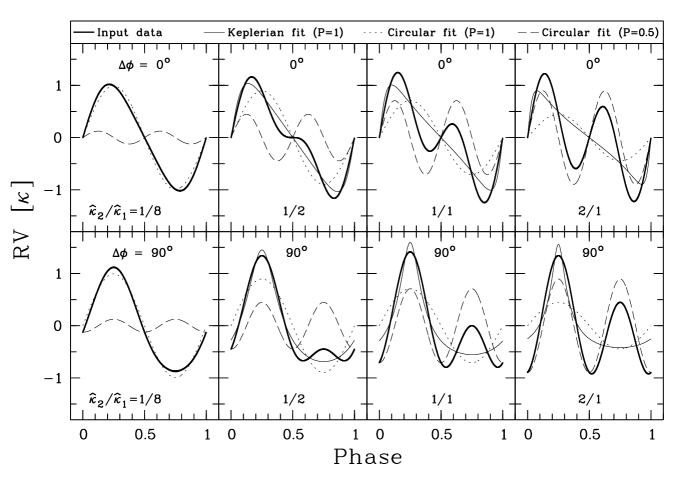
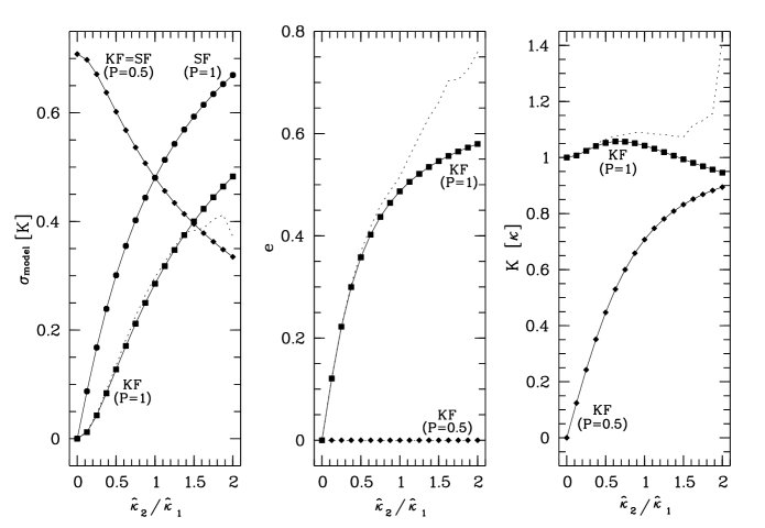
Fig. 1 shows examples of single-planet model fits to the densely sampled simulated input data with different amplitude ratios $\hat{\kappa}_{2}/\hat{\kappa}_{1}$ and two selected values of the phase shift $\Delta\phi=0^{\circ}$ and $90^{\circ}$, while Tab. 1 shows the mean rms deviation $\sigma_{\mathrm{model}}$ of these model fits from the data where the mean has been taken over all 12 phase shift values (see Sect. 3.2 on the relatively small variation of the individual values of $\sigma_{\mathrm{model}}$ as a function of the phase). Actually, as can be seen from Fig. 2 (left panel), the single Keplerian always yields the best fit, i.e. the smallest $\sigma_{\mathrm{model}}$, for $\hat{\kappa}_{2}/\hat{\kappa}_{1}<1.5$, while for $\hat{\kappa}_{2}/\hat{\kappa}_{1}\geq 1.5$ the fit with $P=0.5$ is better.

Figure 4: Rms scatter $\sigma_{\mathrm{Kep}}$ of the RV solutions around single-planet Keplerian fits for our sample of 254 stars for which the EOD provides these values (dots). The scatter values are plotted as a function of the formal eccentricity of the Keplerian fit and in units of its RV semi-amplitude. $1\sigma$–errors of the eccentricity are represented by grey horizontal bars. In two instances no errors are available; the pertinent data points are marked by small circles around them. The large circle and cross marks the case of HD 27894 that is studied in Sect. 4.3. The solid curve is identical to the solid line in Fig. 3 representing the deviation $\sigma_{\mathrm{model}}$ between the single-planet Keplerian model and the model for the 2:1 resonant pair of planets. Scatter values above the curve are larger than the expected deviation arising from applying the erroneous model (single Keplerian instead of 2:1 resonant pair) so that both models are possible, whereas scatter values below the curve are too small to assume an erroneous model and therefore favour the single Keplerian.

Specifically, for an amplitude ratio $\hat{\kappa}_{2}/\hat{\kappa}_{1}=1/8$ (Fig. 1, left panels), the data (thick solid line) and the Keplerian fit with the period of the outer planet (thin solid line) become indistiguishable in our plot, whereas the single sinusoidal fit with the same period (dotted line) can be seen to systematically deviate from the data, and the fit with the period of the inner planet (dashed line) is completely inadequate. For an amplitude ratio of $1/2$ (Fig. 1, second column of panels), the single Keplerian with the period of the outer planet deviates systematically from the data, but could still be a reasonable match to real data, if signal-to-noise ratios are moderate. For this amplitude ratio, the sinusoidal fit with the period of the outer planet deviates much more from the data, and the fit with the period of the inner planet deviates even more (but less than for the amplitude ratio of $1/8$). For an amplitude ratio of $1/1$ (Fig. 1, third column of panels), all single-planet fits are inadequate, but the Keplerian fit with the period of the outer planet is still the formally best fit. For this amplitude ratio, the sine fits with $P=1$ and $P=0.5$ are of equally poor quality since they have the same rms deviation (see Tab. 1). If the amplitude ratio of the inner vs. the outer planet is reversed then for $\hat{\kappa}_{2}/\hat{\kappa}_{1}\geq 1.5/1$ the fit with the period of the inner planet is the best one, followed by the Keplerian fit with the period of the outer planet, and then the sine fit with the period of the outer planet (see Fig. 1, right panels which are for $\hat{\kappa}_{2}/\hat{\kappa}_{1}=2/1$).

3.2 Limited dependence on phase shift

For the densely sampled data sets, we find that the interesting fit parameters RV semi-amplitude $K$ and eccentricity $e$, and also the rms of the fit vary as a function of phase shift $\Delta\phi$ only by very small amounts. For the extreme amplitude ratio $\hat{\kappa}_{2}/\hat{\kappa}_{1}=2$, these variations are $0.55\%$, $1.5\%$, and $8.0\%$ peak-to-valley, respectively, for the rms, for $K$, and for $e$. For smaller amplitude ratios, these values are even smaller. Therefore, in our analysis, for every given amplitude ratio, we are using the mean values for the rms and for $e$ and $K$ obtained from the fits to the 12 data sets with different phase shifts (see Sect. 3.1). For the sparsely sampled data sets, we use the median values (instead of the mean values) of $e$ and $K$ for all further comparisons, since they display somewhat stronger variations and can have strong outliers so that the median is the more representative value.

3.3 Zero eccentricity in P = 0.5 fits

We also find that in the case of the Keplerian models with period $P=0.5$ all fits to the densely sampled data sets yield an eccentricity $e=0$ and an amplitude and rms equal to that of the sine fits with the same period value. That is why we will henceforth no longer distinguish between Keplerian fits and sine fits for $P=0.5$. As noted above, we have not made any fits with $P=0.5$ to the sparsely sampled data sets. In this case, the Keplerian fit with $P=0.5$ will normally show differences from the circular fit, since the sparse sampling does no longer guarantee the symmetric distribution of the radial velocities which is naturally present for a densely sampled sine wave. However in this paper, we will largely concentrate on cases of small deviations from the single sinusoidal model, such as low-eccentricity Keplerians or small-amplitude second circular planets with half the period of the (circular) first one. Consequently, we are exploring the regime where $P=0.5$ fits alone are never a good match anyway.

3.4 Dependence of rms, e, and K on amplitude ratio for dense sampling

This behaviour can also be deduced from Fig. 2 which shows the dependence of the rms of the different types of fits on the amplitude ratio of the input data (left panel). Fig. 2 also shows the variation of the eccentricity $e$ (middle panel) and the semi-amplitude $K$ of the Keplerian fit (right panel) with this ratio.

3.5 Example for dependence of rms, e, and K on amplitude ratio for sparse sampling

In the three panels of Fig. 2, thin dotted lines show the results from the data sets simulated using the sparse sampling example outlined in Sect. 2.2. With this example, we illustrate that conclusions concerning the goodness-of-fit, the determined eccentricity, and the RV semi-amplitude drawn from our idealized densely sampled data are likely to hold also for realistic data sets as long as the RV amplitude ratio $\hat{\kappa}_{2}/\hat{\kappa}_{1}$ of the 2:1-RCO planets is not too large. In particular, our sparse data example and our dense data sets produce similar $\sigma_{\mathrm{model}}$ values for amplitude ratios $\hat{\kappa}_{2}/\hat{\kappa}_{1}$ up to $\approx 1.4$, and similar $e$ and $K$ values for $\hat{\kappa}_{2}/\hat{\kappa}_{1}$ up to $\approx 0.5$ (see Fig. 2).

3.6 Dependence of rms on e – a first tool to search for erroneous models

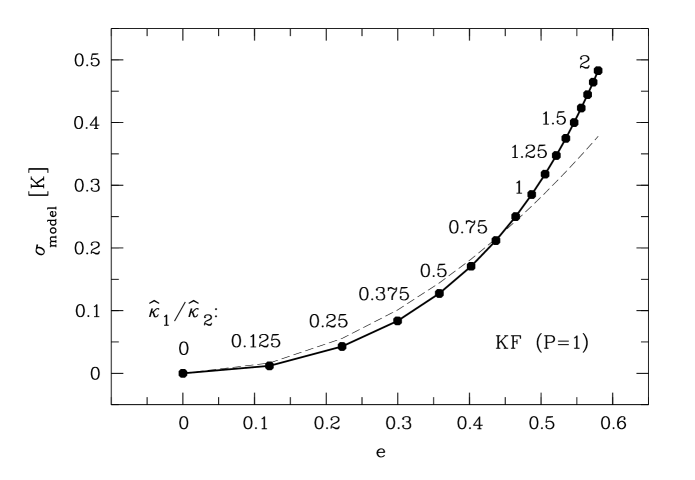
Fig. 3 shows the rms deviation of the Keplerian fit with $P=1$ from the simulated 2:1-RCO data as a function of the pertinent value for the eccentricity obtained by the same fit. This is based on the densely sampled data. We will use this relation as a tool to identify those of the known RV determined planetary systems for which single objects on eccentric orbits have been fitted, but a pair of 2:1 resonant planets is also a possible model.

Looking, in observed data (with not too sparse sampling and moderate amplitude ratios; see Sect. 3.5), at the scatter $\sigma_{\mathrm{Kep}}$ of the RV measurements around the fitted Keplerian model (expressed in units of the RV semi-amplitude $K$ of the fit), Fig. 3 allows us to determine the expected (typical, average) contribution $\sigma_{\mathrm{model}}$ to the scatter arising from the wrong model fit. This means that all systems that we can identify in the literature which have a planet in a putative eccentric orbit as well as a scatter of the data around the eccentric model larger than the one given by the solid curve in Fig. 3 are potential candidates for a 2:1 resonant pair of planets.

In principle, the instrumental noise $\sigma_{\mathrm{inst}}$ and the RV jitter $\sigma_{\mathrm{star}}$ arising from stellar effects such as activity, convective motions, and pulsations, commonly named ‘stellar jitter,’ should also be added in quadrature to the scatter due to the wrong model fit. Systems with an observed RV scatter $\sigma_{\mathrm{Kep}}$ exceeding this combined scatter would then be candidates for a follow-up study in search for a 1:2 resonant second planet, i.e. sytems with $\sigma_{\mathrm{Kep}}^{2}\geq\sigma_{\mathrm{model}}^{2}+\sigma_{\mathrm{inst}}^{2}+\sigma_{\mathrm{star}}^{2}$. In practice, however, this can be done only for those systems for which good estimates of the instrumental noise and of the stellar noise are available. Estimates of the instrumental noise can often be obtained from a joint analysis of the data of the ensemble of stars observed in a survey-type programme, e.g. by looking for the most constant stars, but even for those substantial effort is required to disentangle the instrumental noise from stellar jitter. Short-term jitter due to stellar p-mode oscillations can be estimated using the scaling relation from Kjeldsen & Bedding (1995). There is also quite some literature on estimates of the effects of stellar activity (e.g. Boisse et al. (2011); Saar & Donahue (1997); Saar et al. (1998); Saar & Fischer (2000)), but because of the nature of this activity (spot migration, activity cycles, etc.) they cannot be very precise.

3.7 Probability of chi-square – the tool of choice for real data

As already alluded to in Sect. 2.1, it should be noted that the scatter alone is not a statistically sound criterion, since in general, it is possible to find signals that are smaller than the scatter/noise, if one has a sufficiently large number of measurements. Rather than looking at the rms, the appropriate approach would be to look at the probability of $\chi^{2}$ of the fitted models, and in fact our main data base for planetary orbital parameters (the EOD; see Sect. 4) provides values of $\chi^{2}$ (along with the also required values for the degrees of freedom, DoF) for a good fraction of the interesting entries, but only so for the Keplerian fit, not for an alternative fit with a 2:1 resonant pair of sinusoids.

3.8 First harmonic of the Fourier expansion of the Kepler equation

Anglada-Escudé et al. (2010) base much of their study of 2:1 resonant vs. Keplerian models on the Fourier expansion of the Kepler equation. While we have adopted a different approach in our simulations, a comparison is in order at this point. It is given by the dashed line in Fig. 3 which represents the amplitude of the first harmonic of the Fourier expansion of the Kepler equation (from Anglada-Escudé et al. (2010) and Lucy (2005)). The similarity between the two curves in Fig. 3 demonstrates that the ability to distinguish between the Keplerian model and the model with the 2:1 resonant pair of circular orbits is largely equivalent to the ability to detect this first harmonic.

Figure 5: Cumulative histogram of $\log[p(\chi_{\mathrm{Kep}}^{2})]$ of the Keplerian fits for those $187$ stars in our sample for which both the reduced chi-square $\chi^{2}_{\nu}$ of the fit and the number of measurements is provided by the EOD. For a substantial fraction of the stars, the chi-square probability is too small to accept the single Keplerian model, e.g. $39\%$ of the stars have $\log[p(\chi_{\mathrm{Kep}}^{2})]<-3$ (see also Tab. 2).

3.9 The model-related scatter in real data

We also note that the so determined model-related contributions $\sigma_{\mathrm{model}}$ to the scatter are exact only for very densely sampled RV curves such as those we have used for our simulations (Sect. 2.1). For much more sparsely sampled real data, the model-related contributions to the scatter can deviate somewhat in the individual case from the here determined values. Typically, data sets with fewer measurements can be fitted ‘better’ by any multi-parameter model, so that the model-related contribution to the rms scatter is likely to be somewhat smaller than what we have determined for our simulated data sets with $1000$ equidistant data points. Nevertheless, we will conservatively use these larger values to guide us in our search for candidate systems (i.e. systems with even larger scatter).

4 Follow-up candidates from the literature

4.1 Sample definition

In order to come up with a compilation of candidate systems, we used the Exoplanet Orbit Database (EOD) described by Wright et al. (2011) and available on-line at http://www.exoplanets.org. From the list of detected exoplanets, we have selected two versions of a sample of stars based on the following criteria.

1. Stars with an RV orbital solution.

2. Stars for which no planetary transits have been observed.

3. $e>0$.

4. Listed number of components equal to one (supposedly single planets).

5. $K$ must be given.

6. a) Values for the rms scatter of the data around the a)  Keplerian fit $\sigma_{\mathrm{Kep}}$ are available.
   b) Values for the probability of chi-square $p(\chi_{\mathrm{Kep}}^{2})$ can be b)  obtained from the data base as it provides both the re- b)  duced $\chi^{2}$ and the number of observations.

As of January 13th, 2015, we find that $254$ of the stars contained in the EOD fulfill criteria $1-5$ plus 6a; these will make up our version 1 sample. $187$ of the stars fulfill criteria $1-5$ plus 6b and will constitute our version 2 sample. $185$ stars fulfill criteria $1-5$ plus 6a and 6b. Concerning criterion 6b, we note that the EOD contains entries for the (reduced) chi-square $\chi_{\mathrm{Kep}}^{2}$ and the number of measurements $N$ from which we determine $p(\chi_{\mathrm{Kep}}^{2})$ using standard routines (e.g. Bevington (1969)).

Note that in order to constrain the sample, we discarded known transiting systems (criterion 2), since for those chances are higher that a second planet further inside in the system has already been detected through its own transits. We also restricted ourselves to supposedly single-planet systems (criterion 4), because finding an additional low-amplitude planet in a 2:1 resonance with one of the planets in the system will be more difficult when more than one planet has already been found to contribute to the observed stellar RV signal.

Table 2: Suitability of the single Keplerian model alone, i.e. assuming that no other sources of variability exist. Second row: number of stars for which the chi-square probability of the single Keplerian model is less than the values given in the first row. Third row: fraction of the $187$ stars in our version 2 sample. Last row: confidence $C=1-p(\chi^{2}_{\mathrm{Kep}})$ with which the single Keplerian model can be rejected.

$p(\chi^{2}_{\mathrm{Kep}})$	$<0.05$	$<0.01$	$<0.005$	$<0.001$
No. of stars	$101$	$83$	$79$	$72$
Fraction	$54\%$	$44\%$	$42\%$	$39\%$
Confidence $C$	$>95\%$	$>99\%$	$>99.5\%$	$>99.9\%$

Figure 6: Fit to the HD 27894 RVs with a model consisting of two planets in circular orbits. Note that in this case the exact 2:1 resonance is not forced, but the two period values are both free parameters of the fit.   —  Left: Time series together with the best-fitting two-planet circular model (top, thick solid line) and residuals (bottom). For display purposes the x-axis has been broken between BJD - 2,452,950 and BJD - 2,453,267.5 where there is a large data gap. The thin dashed line in the upper panel represents the best-fitting single Keplerian model for comparison.   —  Right: RV data phase folded with the period of the outer planet after subtraction of the signal of the inner planet (top) and phase folded with the period of the inner planet after subtraction of the signal of the outer planet (bottom).

4.2 Resulting candidate sample

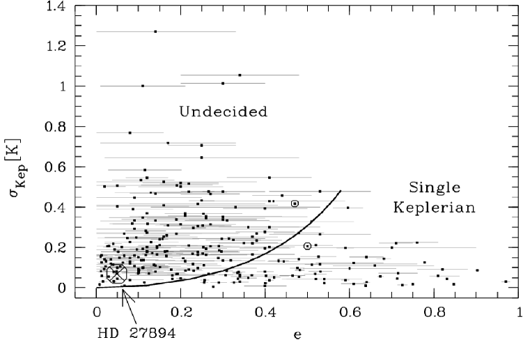
Fig. 4 shows the location in the rms-vs.-eccentricity diagram of our version 1 sample stars in comparison to the curve from Fig. 3, i.e. the curve that depicts the expected contribution to the rms if a 2:1 resonant system with two circular orbits is fitted with a single-star Keplerian model. We find that $188$ of the $254$ stars in the sample are located above the curve, i.e. $74\%$ of the stars are possible candidates for hosting a system of two planets in a 2:1 resonance when the criterion of exceeding the model-related scatter for 2:1-RCO systems is applied (see Sect. 3.6).

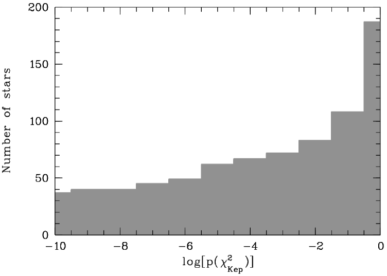
In order to apply also the probability of $\chi^{2}$ of the single Keplerian fits as a criterion for identifying candidates (Sect. 3.7), we display in Fig. 5 (on a logarithmic abscissa) the cumulative histogram of $p(\chi_{\mathrm{Kep}}^{2})$ for our version 2 sample stars which demonstrates that a large fraction of the stars has a very low probability that the applied model alone is correct. This is also shown by Tab. 2 that lists how many stars have $p(\chi_{\mathrm{Kep}}^{2})<0.05,\leavevmode\nobreak\ <0.01,\leavevmode\nobreak\ <0.005$, and $<0.001$, respectively, and which fraction of the total of $187$ stars in our version 2 sample this corresponds to. It also provides the confidence for the rejection of the single Keplerian model for these stars given by $1-p(\chi_{\mathrm{Kep}}^{2}$). The hypothesis that the Keplerian model alone can explain the observed variability can be rejected for $54\%$ of our version 2 sample stars at the $95\%$ confidence level and for $39\%$ at the $99.9\%$ confidence level.

4.3 A case study: HD 27894

From our (version 1) sample of candidate 2:1-RCO systems (systems above the curve in Fig. 4), we selected the 20 very sparsely sampled RV measurements of HD 27894 (Tab. A.2 in Moutou et al. (2005)) in order to provide an example for a detailed study of a supposedly single-planet system which might hide a second planet in an inner orbit near a 2:1 MMR with the first one. (We have already employed the observing times of this star in Sect. 2.2.) HD 27894 is a low-activity K2V star with a mass of $0.8\leavevmode\nobreak\ \mathrm{M}_{\odot}$. Further characteristics of the star are described in Moutou et al. (2005).

HD 27894 was selected because the moderate eccentricity of the published Keplerian fit as well as the considerable scatter of the data around it made this system a perfect candidate for an ambiguous, undecided case well suited for an illustrating example. This system earns much of this ambiguity from its very sparse data sampling.

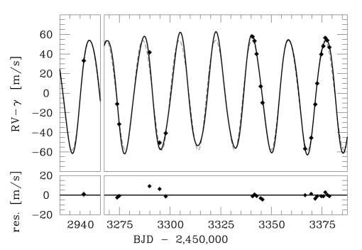
We base our analysis of the HD 27894 system on various models. First we apply a single Keplerian fit just like Moutou et al. (2005) and obtain fit parameters in agreement with those found by these authors (except for a $2\leavevmode\nobreak\ \mathrm{m\leavevmode\nobreak\ s}^{-1}$ offset in the systemic RV $\gamma$; see Tab. 3). As discussed in Sect. 1 this model has six free parameters (Eqs. 3 and 4). We find a low-eccentricity fit with a reduced chi-square of $\chi^{2}_{\mathrm{\nu}}=8.706$ (DoF=$14$), hence $p(\chi^{2})=2.69\times 10^{-19}$ implying that the fitted model alone cannot at all describe the data if the measurement errors are reliable. At this point, of course, a multi-planet model is not necessarily called for yet, since stellar RV jitter (due to pulsations, convection, and activity) could also be responsible for the excess variability; see the pertinent discussion in Moutou et al. (2005) on the fact that the adopted average RV error of $1.8\leavevmode\nobreak\ \mathrm{m\leavevmode\nobreak\ s}^{-1}$ does not take stellar variability into account. The single Keplerian fit has an rms of $4.21\leavevmode\nobreak\ \mathrm{m\leavevmode\nobreak\ s}^{-1}$ and yields a minimum companion mass of $m\sin i=0.645\leavevmode\nobreak\ \mathrm{M}_{\mathrm{Jup}}$ and an orbital period of $P=17.99\leavevmode\nobreak\ \mathrm{d}$ (Tab. 3).

Next we consider two-planet fits. We start off with the exact 2:1-RCO case which yields values for the orbital period and planetary mass for the outer planet very close to those found for the single-Keplerian model (Tab. 3) and only a small improvement of chi-square, $\chi^{2}_{\nu}=8.581$, $p(\chi^{2})=5.92\times 10^{-19}$ (DoF $=14$) and rms ($4.17\leavevmode\nobreak\ \mathrm{m\leavevmode\nobreak\ s}^{-1}$). In this model, the inner planet has $m\sin i=8.4\leavevmode\nobreak\ \mathrm{M}_{\mathrm{Earth}}$. The similarity of the 2:1-RCO fit with the single Keplerian demonstrates the ambiguity of the model selection in this case of sparsely sampled RV data.

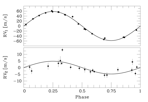
The situation changes somewhat when we leave the two period values free but retain circular orbits (eccentricities $e_{1}=e_{2}=0$, hence $\omega_{1}$ and $\omega_{2}$ are undefined). Our new model now has seven free parameters, one more than Eq. (1) or (2) since here we are not forcing the 2:1 ratio for the periods. The resulting fit corresponds to a two-planet system with $P_{1}=17.9919\leavevmode\nobreak\ \mathrm{d}$, $m_{1}\sin i=0.648\leavevmode\nobreak\ \mathrm{M}_{\mathrm{Jup}}$, $P_{2}=8.276\leavevmode\nobreak\ \mathrm{d}$, and $m_{2}\sin i=0.044\leavevmode\nobreak\ \mathrm{M}_{\mathrm{Jup}}=14\leavevmode\nobreak\ \mathrm{M}_{\mathrm{Earth}}$ (see Tab. 3 and Fig. 6). The two-planet fit has a substantially smaller $\chi^{2}_{\mathrm{\nu}}=5.444$ (DoF=$13$), but still a very small $p(\chi^{2})$ of $2.37\times 10^{-19}$, probably since stellar jitter is dominating the noise behaviour but is not considered in the model. The rms of the fit is $3.20\leavevmode\nobreak\ \mathrm{m\leavevmode\nobreak\ s}^{-1}$. Applying an F-test to the $\chi^{2}$ ratio of the fits, we find a relatively moderate confidence of $83\%$ that this new model is an improvement over either the single Keplerian or the 2:1-RCO models (same confidence value in both cases). If the F-test is applied to the rms’s of the fits, a similar value of $82\%$ is obtained in both cases.

We then study the orbital stability of the possible two-planet system following an approach similar to the one outlined in Trifonov et al. (2014). We perform N-body simulations employing the symplectic integrator SyMBA (Duncan et al. 1998) which is particulary suited to treat close encounters between the planets. The fitting code is described in detail in Tan et al. (2013).

For these simulations we assumed co-planar orbits seen edge-on for both planets, i.e. the orbital inclinations are $i_{1}=i_{2}=90^{\circ}$. The initial orbital elements are obtained in the Jacobi frame matched to the representation of hierarchical multi-planet systems (see Lee & Peale (2003)). Our choice of co-planar edge-on orbits can be motivated as follows. First, if nothing is known about the orbital inclination and random orientation is assumed, $90^{\circ}$ is the most probable value. Second, for this inclination value the planet mass is equal to its minimum mass determined from the RV data. While higher mass planets will have a stronger gravitational interaction and can potentially disturb each other more, edge-on orbits are the relevant ones for the question whether there are stable orbits at all. Third, while co-planarity maximizes the interaction between the planets, co-planar orbits are nevertheless thought to be the predominant configuration for planetary systems originating from a circumstellar disk. This leads us to assume them here.

Table 3: Orbital parameters for the HD 27894 system for the various applied models. $N_{\mathrm{par}}$ is the number of model parameters and $\mathrm{DoF}=N_{\mathrm{data}}-N_{\mathrm{par}}$ the number of degrees of freedom (with $N_{\mathrm{data}}$ the number of data points). All model parameters from $P_{1}$ to $\gamma$ are as defined for Eqs. (1-4). Framed values were held fixed for the fits. $m_{1}\sin i$ and $m_{2}\sin i$ are the derived minimum masses of the outer and inner planet, respectively, $a_{1}$ and $a_{2}$ the pertinent semi-major axes of the orbits.

	1-planet models		2-planet models
	Moutou et al.	This work	This work
	(2005)		2:1-RCO	2-pl. circular
	single	single	$e_{1}=e_{2}=0$	$e_{1}=e_{2}=0$	Double
	Keplerian	Keplerian	$P_{1}=2P_{2}$	$P_{1}\not=2P_{2}$	Keplerian
$N_{\mathrm{par}}$	6	6	6	7	11
$P_{1}$          $[\mathrm{d}]$	$17.991\pm 0.007$	$17.9904\pm 0.0077$	$17.9915\pm 0.0071$	$17.9919\pm 0.0070$	$17.99\pm 0.35$
$P_{2}$          $[\mathrm{d}]$	—	—	$P_{1}/2$	$\leavevmode\nobreak\ 8.276\leavevmode\nobreak\ \leavevmode\nobreak\ \pm 0.035\leavevmode\nobreak\$	$\leavevmode\nobreak\ \leavevmode\nobreak\ 8.27\pm 0.99$
$t_{\mathrm{p,1}}$         $[\mathrm{BJD}-2450000]$	$2933.7\pm 0.5^{(a)}$	$2933.64\pm 0.55$	—	—	$2928.2\pm 1.6$
$t_{\mathrm{p,2}}$         $[\mathrm{BJD}-2450000]$	—	—	—	—	$2933.8\pm 5.9$
$t_{\mathrm{max,1}}$      $[\mathrm{BJD}-2450000]$	—	—	$2926.98\pm 0.16$	$2927.03\pm 0.16$	—
$t_{\mathrm{max,2}}$      $[\mathrm{BJD}-2450000]$	—	—	$2939.40\pm 0.25$	$2941.60\pm 1.75$	—
$e_{1}$	$0.049\pm 0.008$	$0.0486\pm 0.0086$	$0$	$0$	$0.057\pm 0.021$
$e_{2}$	—	—	$0$	$0$	$0.532\leavevmode\nobreak\ \pm 0.076\leavevmode\nobreak\$
$\omega_{1}$             $[^{\circ}$]	$132.9\pm 9.7\leavevmode\nobreak\ \leavevmode\nobreak\$	$132\pm 11$	—	—	$20.1\pm 24.6$
$\omega_{2}$             $[^{\circ}$]	—	—	—	—	$30.8\pm\leavevmode\nobreak\ \leavevmode\nobreak\ 8.0$
$K$ or $\kappa_{1}^{(b)}$    $[\mathrm{m\leavevmode\nobreak\ s}^{-1}]$	$58.1\pm 0.5$	$58.13\pm 0.50$	$58.02\pm 0.50$	$58.28\pm 0.49$	$57.57\pm 0.60$
$\kappa_{2}$ or $K_{2}^{(b)}$  $[\mathrm{m\leavevmode\nobreak\ s}^{-1}]$	—	—	$\leavevmode\nobreak\ \leavevmode\nobreak\ 3.00\pm 0.51$	$\leavevmode\nobreak\ \leavevmode\nobreak\ 5.17\pm 0.62$	$\leavevmode\nobreak\ \leavevmode\nobreak\ 8.24\pm 1.33$
$\gamma$               $[\mathrm{km\leavevmode\nobreak\ s}^{-1}]$	$82.9023$	$82.90033$	$82.90225$	$82.90231$	$82.90179$
	$\pm 0.0003$	$\pm 0.00057$	$\pm 0.00036$	$\pm 0.00039$	$\pm 0.00053$
$m_{1}\sin i^{(c)}$  $[\mathrm{M}_{\mathrm{Jup}}]$	$0.62$	$0.645$	$0.645$	$0.648$	$\leavevmode\nobreak\ \leavevmode\nobreak\ 0.639$
$m_{2}\sin i^{(c)}$  $[\mathrm{M}_{\mathrm{Jup}}]$	—	—	$0.026$	$0.044$	$\leavevmode\nobreak\ \leavevmode\nobreak\ 0.060$
$m_{2}\sin i^{(c)}$  $[\mathrm{M}_{\mathrm{Earth}}]$	—	—	$8.4$	$14$	$19$
$a_{1}^{(c)}$            $[\mathrm{AU}]$	$0.122$	$0.125$	$0.125$	$0.125$	$0.125$
$a_{2}^{(c)}$            $[\mathrm{AU}]$	—	—	$0.079$	$0.074$	$0.074$
rms           $[\mathrm{m\leavevmode\nobreak\ s}^{-1}]$	$4.0$	$4.21$	$4.17$	$3.20$	$2.42$
$\chi^{2}_{\nu}$	not given	$8.706$	$8.581$	$5.444$	$2.522$
DoF	$14$	$14$	$14$	$13$	$9$
$p(\chi^{2}_{\nu})$	not given	$2.69\times 10^{-19}$	$5.92\times 10^{-19}$	$2.37\times 10^{-19}$	$6.91\times 10^{-3}$
Stability	n.a.	n.a.	Yes	Yes	No(d)

Notes:	(a) Moutou et al. (2005) quoted a value of $3275.5\pm 0.5$, which is later by $19$ revolutions of the planet.
	(b) As in the text, $K$ stands for the semi-amplitude of the single Keplerian, wheras $\kappa_{1}$ and $\kappa_{2}$ stand for the semi-amplitudes of the
	circular orbits of the outer and inner planet, respectively; $K_{2}$ is meant to denote the semi-amplitude of the inner planet in the
	double Keplerian fit (last column).
	(c) All determinations of $m\sin i$ and $a$ made in this work use a stellar mass of $0.8\leavevmode\nobreak\ \mathrm{M}_{\odot}$. Contrary to their claim of having used the
	same value, Moutou et al. (2005) must have adopted $0.75\leavevmode\nobreak\ \mathrm{M}_{\odot}$ in order to arrive at their somewhat smaller $m_{1}\sin i$ and $a_{1}$.
	(d) Stable only if $e_{2}$ is constrained to $<0.3$ (for the case $i_{1}=i_{2}=90^{\circ}$).

Figure 7: Orbital evolution of the best-fit system of two planets that started off on circular orbits but with unconstrained periods.   —  Left: 1-year excerpt from the simulation.   —  Right: excerpt for the following $999\leavevmode\nobreak\ \mathrm{yr}$. Both in the left and right part of the figure, the individual panels show from top to bottom the short-term variation of the semi-major axes $a_{1}$ and $a_{2}$, of the eccentricities $e_{1}$ and $e_{2}$, and of the difference of the longitudes of periastron $\omega_{2}-\omega_{1}$. The last quantity is not plotted when one of the eccenticities are close to zero ($e_{1}$ or $e_{2}<0.0001$) since then the longitude of periastron is undefined (hence the gaps in the lower left panel). The variation pattern of these parameters shows various periodicites of which the following can be most easily seen here: $15\leavevmode\nobreak\ \mathrm{d}$ and $104\leavevmode\nobreak\ \mathrm{d}$ (all five parameters, left part of figure), and $65\leavevmode\nobreak\ \mathrm{yr}$ ($e_{1}$ and $\omega_{2}-\omega_{1}$; right part of figure).

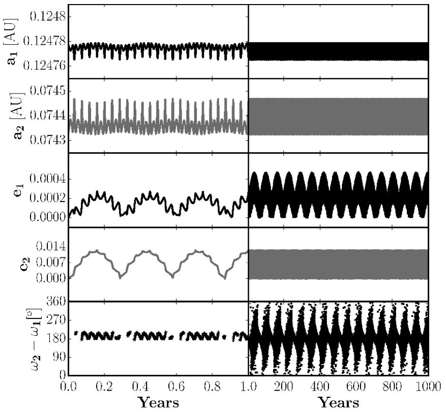
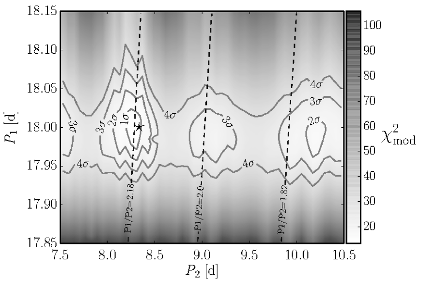
We find the best fit with initially two circular orbits and free period values to be stable over the complete simulation time span of $10000\leavevmode\nobreak\ \mathrm{yr}$ corresponding to over $2.3\times 10^{5}$ and $4.6\times 10^{6}$ orbits of the outer and inner planet, respectively. A $1\leavevmode\nobreak\ \mathrm{yr}$ and a (contiguous) $999\leavevmode\nobreak\ \mathrm{yr}$ excerpt from the simulation are shown in Fig. 7 and reveal very regular oscillations (on several time scales) of the semi-major axes, the eccentricities, and the difference of the longitudes of periastron of the two planets. The amplitudes of these oscillations are small. The semi-major axes of the outer and inner planet vary by about $10^{-4}$ and $2\times 10^{-4}$, repectively. Only very small eccentricity values are reached ($0\leq e_{1}\leq 0.00045$ and $0\leq e_{2}\leq 0.013$). With a period ratio of $P_{1}/P_{2}=2.17$, this system is not exactly in 2:1 MMR but still in the range of period ratios within $\pm 9\%$ of the MMR found to be frequent by Lissauer et al. (2011) in Kepler data (see Sect. 1 above). It is particularly noteworthy that this period ratio is very close to the value of 2.2 where a significant excess of planet pairs was found by Steffen & Hwang (2015) also in Kepler data (Sect. 1).

In order to check whether a system starting off at period ratios near 2:1 (including the exact ratio) can also be stable, we examine a high density ($50\times 50$ fits) $\chi^{2}$ grid of two-planet circular fits with different initial periods. We have tested each fit for long-term stability. The result is shown in Fig. 8 which shows a modified chi-square defined to be equal to DoF at its minimum by $\chi^{2}_{\mathrm{mod}}=\mathrm{DoF}\cdot\chi^{2}/\chi^{2}_{\mathrm{min}}$. Note that all models on this map are stable, and so is the one starting at the exact 2:1 period ratio which is also consistent with the optimum fit (at $\chi^{2}_{\mathrm{min}}$) at better than the $3\sigma$ level; more precisely, it lies within the combined $3\sigma$ error regime for the interesting parameters $P_{1}$ and $P_{2}$ around the optimum fit (cf. Lampton et al. (1976); also Avni (1976)).

Finally, we fit the eccentric two-planet model to the data. First we apply the double Keplerian model, but we are unable to constrain the eccentricity of the inner planet (perhaps due to the sparse data sample). The best-fitting double Keplerian has $\chi^{2}_{\nu}=2.522$ and $p(\chi^{2})$ of $6.91\times 10^{-3}$ (DoF $=9$; see Tab. 3 for the fit parameters). When comparing it with the 6-parameter single Keplerian and 2:1-RCO models, an F-test applied to the $\chi^{2}$ ratios shows that in both cases there is a confidence of $99\%$ that the five additional parameters of the double Keplerian provide a significant improvement of the fit. When the F-test is applied to the ratio of the squared rms’s, this confidence is $95\%$ in both cases. However, the best-fitting double Keplerian yields a very large value for the eccentricity of the inner planet of $e_{2}=0.51$. Not only does this value have an enormeous uncertainty of $\pm 0.47$, it also leads to a highly unstable planetary configuration. In order to exclude such unstable models by imposing stability constraints, we apply a self-consistent two-planet N-body model (Laughlin & Chambers (2001); Tan et al. (2013)). We find that, if we constrain the eccentricity of the inner planet to $e_{2}<0.3$, we arrive at a stable orbit again.

Comparing the models we have studied in this subsection we certainly find some preference for a two-planet model for the HD 27894 system even though this is not fully conclusive yet. This is mainly due to the sparseness of the available data. Since the formal best fit with two Keplerians drives the eccentricity of the potential inner planet to values so high that the system becomes unstable, models with moderate eccentricities should be preferred. This includes the model with two circular orbits. HD 27894 is clearly an example for a system where more observations hold the potential to uncover a second planet.

Figure 8: Map of modified chi-square, $\chi^{2}_{\mathrm{mod}}=\mathrm{DoF}\cdot\chi^{2}/\chi^{2}_{\mathrm{min}}$, as a function of the two orbital periods of the two-circular-planets model for HD 27894. All models on this map are stable. Contours are combined confidence levels with respect to the best fit, i.e. the $1,\leavevmode\nobreak\ 2,\leavevmode\nobreak\ 3$ and $4\leavevmode\nobreak\ \sigma$ regimes in which both period values are found together with a probability of $68.27\%$, $95.45\%$, $99.73\%$, and $99.99\%$, respectively (while the remainder of the orbital parameters is optimized, i.e. treated as uninteresting). The best fit with $\chi^{2}_{\mathrm{mod}}=\mathrm{DoF}=13$ is denoted by an asterisk. It is within the $\pm 9\%$ region from the exact 2:1 period ratio. The left and right slanted dashed lines delimit this region whereas the middle one marks the exact ratio. Exact 2:1 solutions are found within the $3\leavevmode\nobreak\ \sigma$ contour (middle). The $1,\leavevmode\nobreak\ 2,\leavevmode\nobreak\ 3$ and $4\leavevmode\nobreak\ \sigma$ contours correspond to $\chi^{2}_{\mathrm{mod}}=15.30,\leavevmode\nobreak\ 19.18,\leavevmode\nobreak\ 24.83$, and $32.33$, respectively.

5 Discussion

5.1 Observational strategy for the follow-up

In this paper we have illustrated how RV data with uncertainties can lead observers to apply the wrong model for the description of the data of planet hosting stars. In particular, we have concentrated on the topic of the erroneous application of a single Keplerian one-planet model instead of a 2:1 resonant two-planet model. Sparse sampling as well as insufficient measurement precision can make it difficult to distinguish between the two models. Sparse sampling may just not cover enough of those orbital phases where the two models differ most, and measurement errors may be too large for attempts to resolve the difference between the models.

Naturally, improvement will come from more observations of the candidate stars, and even more so if also the measurement precision can be improved. Observational methods other than RV measurements, such as astrometry or photometric transits can contribute to the selection of the best model for the studied planetary system. McArthur et al. (2014) provide an example for employing constraints from astrometry and photometry to distinguish between or exclude certain models. Mostly though, the follow-up will consist of securing more RV measurements. These can be optimized based on the following recipe:

• Fill phase gaps in the data.

• Preferentially observe those phases of the RV curve where the differences between the models are strongest.

On average, doubling the number of measurements increases the ability to resolve the difference between the models by a factor of $\sqrt{2}$. With higher instrumental precision this ability is even greater provided that the main limitation is not due to intrinsic effects of the star such as activity, convective motions, and pulsations.

To illustrate the best choice of phases by way of example, take the second panel from the left in the upper row of panels in Fig. 1. If one compares the thick solid line, i.e. the 2:1-RCO two-planet model, with the thin solid line, i.e. the Keplerian one-planet model, the largest differences occur at phases near $0.18$, $0.40$, $0.60$, and $0.82$ whereas intermediate phases have smaller discrepancies. Given the usually limited observing time, one should concentrate on those phases of the largest differences.

5.2 Biased eccentricity distribution and consequences for planetary system formantion

Determining the fraction of two-planet systems near the 2:1 resonance among the systems previously classified as eccentric single-planet ones will allow us to find the degree to which the observed eccentricity distribution is biased. It may turn out that solar-system-like architectures with low-eccentricity planets are more frequent than previously thought. If a significant bias can be established, this will certainly have implications for theories of the formation of planetary systems. We note in this context also that, according to several authors, resonances observed in planetary systems provide clues to planetary migration processes and the architecture of those systems (e.g. Pierens et al. (2014); Delisle & Laskar (2014); Beaugé et al. (2006)).

5.3 Outer planets as perturbers

One related topic is worth mentioning here, even though we have not studied it in this paper. Rodigas & Hinz (2009) investigated the effect that undetected second planets in wide (outer) orbits have on the determined eccentricity value of supposed single planets in sparse RV data. These authors find that a massive outer planet can lead to published eccentricity values for the detected inner planet that are too large. In this way they have a similar effect as the 2:1 resonant inner planet on which we have concentrated in this study.

6 Conclusions

1. We have studied the case that in RV measurements a two-planet system with 2:1 resonant circular orbits (2:1-RCO system) is erroneously interpreted as a single-planet system and fitted with a single eccentric Keplerian.

2. By way of simulation we have determined how, on average, the discrepancy between the true and the false models depends on the eccentricity of the fitted Keplerian.

3. From the excess scatter of the data around the fitted model, we find that in $74\%$ of $254$ stars for which a single eccentric planet was announced a 2:1-RCO system is a possible alternative model that cannot be excluded.

4. Based on the probability of $\chi^{2}$ we, find that for $54\%$ of $187$ stars the Keplerian fit can be rejected as the sufficient model at the $95\%$ confidence level and for $39\%$ of $187$ stars it can be rejected at the $99.9\%$ confidence level.

5. Therefore, a large number of single-planet systems announced in the literature should be scrutinized with follow-up observations in order to provide the data quality needed to distinguish between the two models in question.

6. Conceivably, it may then be further established that a substantial fraction of the supposed single eccentric orbits are in fact near-circular systems of two planets near the 2:1 resonance. This finding would imply a bias in the determined eccentricity distribution making the quasi-circular orbits prevailing in the solar system more frequent than presently thought. This would have direct implications on planet formation theory.

7. Employing the example of HD 27894, we illustrate the model alternatives finding that this star may have a Uranus or Neptune-mass planet in an inner orbit near the 2:1 resonance with its known Jovian planet. Intriguingly, our two-planet models for this star yield a period ratio close to 2.2, a value where an excess of planets pairs is found in data from the Kepler mission.

8. For this system, we also perform stability simulations showing that there are stable orbits at or near the 2:1 MMR when we assume initially circular orbits for both planets.

9. If fully Keplerian orbits are allowed for both the known and the hypothesized planet, the HD 27894 system is only stable when the eccentricity of the inner planet is constrained to $<0.3$.

10. We suggest that follow-up observations of candidate systems should naturally concentrate on those phases of the orbit of the known planet with the strongest discrepancies between the two-planet and the single-planet (Keplerian) models.