AMADA-Analysis of Multidimensional Astronomical Datasets

Abstract

We present AMADA, an interactive web application to analyse multidimensional datasets. The user uploads a simple ascii file and AMADA performs a number of exploratory analysis together with contemporary visualizations diagnostics. The package performs a hierarchical clustering in the parameter space, and the user can choose among linear, monotonic or non-linear correlation analysis. AMADA provides a number of clustering visualization diagnostics such as heatmaps, dendrograms, chord diagrams, and graphs. In addition, AMADA has the option to run a standard or robust principal components analysis, displaying the results as polar bar plots. The code is written in r and the web interface was created using the shiny framework. AMADA source-code is freely available at https://goo.gl/KeSPue, and the shiny-app at http://goo.gl/UTnU7I.

1 Introduction

The emerging precision era of astronomy marks the transition from a data-deprived field to a data-driven science, in which statistical methods play a central role. The need to handle these ever-increasing datasets impacts all branches of modern science, characterizing the so-called era of Big Data. As a consequence, an efficient exploration of high-dimensional datasets is becoming ubiquitous throughout all scientific fields, such as biology (e.g., Venter et al., 2004), social sciences (e.g., Patty and Penn, 2015), geology (e.g., van Zyl, 2014) and astronomy (e.g., Ball and Brunner, 2010; Graham et al., 2013; Martinez-Gomez et al., 2013).

Upcoming surveys such as the Large Synoptic Survey Telescope (e.g., LSST Science Collaboration et al., 2009), the Square Kilometre Array (e.g., Carilli, 2014), and Euclid (e.g., Scaramella et al., 2015), just to mention a few, will push the boundaries of our ability to analyse sky catalogs, while the ever-increasing complexity of cosmological simulations keeps lessening the distance between observed and synthetic data (e.g., Overzier et al., 2013; de Souza et al., 2013b, 2014b; Vogelsberger et al., 2014).

An optimal exploration of these catalogs, observed and/or simulated, heavily relies on our ability to uncover hidden relationships among different quantities (e.g., Borne et al., 2008; Ball and Brunner, 2010; Graham et al., 2013), such as fundamental planes of galaxy properties (Tully and Fisher, 1977; Faber and Jackson, 1976), as well as to identify the optimal set of variables to describe and predict a certain property of interest (e.g. the presence of star formation activity in a halo; de Souza et al. 2015).

A mainstay methodology for data exploration in astronomy is the correlation analysis. Its goal is to describe the level of association, usually linear, between a given pair of variables. Its applicability virtually covers the entire astronomical domain, such as gamma-ray bursts (e.g., Burgess et al., 2014), cosmic voids (Hamaus et al., 2014), star formation activity (Lee et al., 2013), dark matter halo properties (de Souza et al., 2013a, 2014a), and baryonic galaxy properties (Yates et al., 2012), just to cite a few.

To facilitate the use of contemporary exploratory and visualization techniques commonly used in other scientific fields but not fully exploited in astronomy, we developed the AMADA package. The code allows the user to visualize subgroups of variables with high association in a hierarchical tree structure through diverse visual tools, such as graphs, chord diagrams, dendrograms and heatmaps. The goal is to deliver a user-friendly guide for a first data screening. By providing a systematic methodology for clustering detection in the space of object properties, the researcher can make a statistically justified decision about the subset of features to be studied in a given catalog.

It is worth noting that other interfaces for data exploration in astronomy exist (e.g, Brescia et al., 2010; Burger et al., 2013; Konstantopoulos, 2015). Particularly, VOStat (Chakraborty et al., 2013) and AstroStat (Kembhavi et al., 2015) are two web-based services for statistical analysis using R under the hood. Both projects are focused on providing a user-friendly environment to perform a wide range of standard statistical analysis, such as hypothesis testing, multivariate analysis, clustering and so forth. However, AMADA is the first of its kind with a primary focus on information visualization techniques for general correlation analysis in multidimensional catalogs.

2 Main features

AMADA is written in r 3.1.1 and developed using Rstudio and Shiny frameworks. RStudio is an open source interface for development of r applications, and Shiny is a package that allows to build interactive web applications directly from r. Instructions on how to run the code locally, and a brief installation tutorial are given in A.

The package allows an interactive exploration and information retrieval from high-dimensional datasets. The user can choose among different methods for correlation analysis, whose outcomes are displayed in a chosen graphical layout for visual inspection. In the following, we briefly describe the main available features.

2.1 Datasets

The user can upload a dataset in a plain text ascii file as space or comma separated values (CSV). The columns should be named, and missing data should be marked as $NA$. An example of how a typical dataset looks like, together with a screenshot from the web portal, is displayed in Fig. 1. Alternatively, the user can use the download data button to inspect on its own text editor how to format the matrix. The current version of AMADA does not allow an interactive selection of columns. Therefore, we show below how it can be easily done in r command line using the $c$ function:

⬇

1data(iris)

2colnames(iris)<-c("SL","SW","PL","PW","Species")

3head(iris)

4 SL SW PL PW Species

5 5.1 3.5 1.4 0.2 setosa

6 4.9 3.0 1.4 0.2 setosa

7iris2<-iris[,c("SL","SW")]

8head(iris2)

9 SL SW

10 5.1 3.5

11 4.9 3.0

The original column names of the famous iris dataset (Fisher, 1936) are shortened in the example (S = sepal, P = petal, L = length, W = width) to save space.

Figure 1: A screenshot of the AMADA portal showing properties of host galaxies of Type Ia supernovae. This portal is publicly available at http://goo.gl/UTnU7I.

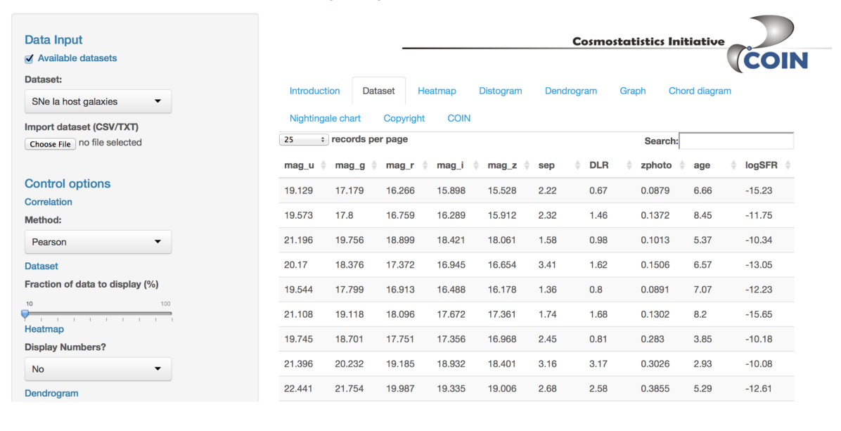
In addition, some public catalogs are already made available on the portal. In the following we will use two of them for explanatory purposes. As an example of low-dimensional and relatively small sample we use a catalog of galaxies experiencing supernova (SN) explosions, while as an example of high-dimensional and moderately large sample we use a mock galaxy catalog. More specifically, we apply AMADA to investigate:

• Supernova host galaxy properties (Sako et al., 2014). In this catalog the properties of Type Ia and II supernova host galaxies are retrieved from the Sloan Digital Sky Survey multi-band photometry. The available catalog represents a sub-sample of the original one, after removal of non-supernova objects and missing data. The final sample is composed of 443 (56) galaxies hosting Type Ia (Type II) supernova, each of them described by 10 parameters, such as galaxy age, star formation rate, distance from supernova to the host galaxy, and so forth.

• Galaxy properties (Guo et al., 2011). A mock galaxy catalog built using semi-analytic galaxy formation models and the N-body Millennium Simulations (Springel, 2005). The initial data set is composed of $\approx 180,000$ haloes at redshift 0. To avoid numerical artifacts due to low resolution effects, we select only those structures with at least $300$ particles (e.g., Antonuccio-Delogu et al., 2010). In addition, we consider only central star forming galaxies (i.e., no satellite galaxies). The remaining dataset is composed of 7079 haloes, and each halo is described by approximately 30 parameters.

As here we adopt the original nomenclature for the various quantities, we recommend the reader to refer to the original articles or catalogs for a detailed description of each parameter.

2.2 Control Options

Several control options are available on the portal to choose among different methods of analysis and visualization. Once the desired combination is chosen, the user should click on the button Make it so! to update the results. The following options are available:

• Fraction of data to display: choose the percentage of data displayed on the screen.

• Correlation method: choose among Pearson, Spearman or Maximum Information Coefficient (MIC).

• Display numbers: choose if correlation coefficients should be displayed in the heatmap.

• Dendrogram type: choose among phylogram, cladogram or fan configurations.

• Graph layout: choose between spring and circular configurations.

• Chord diagram colour: choose among different colour schemes.

• Number of PCs: choose the number or Principal Components (PCs) to display as Nightingale charts.

• PCA method: choose between standard or robust Principal Components Analysis (PCA).

3 Methods

In this section we briefly discuss the different methods used by AMADA to analyse the datasets.

3.1 Correlation methods

The correlation analysis quantifies the strength of the association between a pair of variables, through a correlation coefficient. Its absolute value varies between 0 (uncorrelated variables) and 1 (perfect association). Currently, AMADA offers three options of correlation measurements: linear (Pearson; Pearson, 1895), monotonic (Spearman; Spearman, 1904) and non-linear (MIC; Reshef et al., 2011). We briefly present them in the following, and refer the reader to the original papers for more details.

Pearson

This is widely employed in statistics to measure the degree of the relationship between linearly related variables. The following formula is used to estimate the Pearson coefficient, $r_{p}$, between two variables $X_{i}$ and $Y_{i}$:

$$r_{p}=\frac{\sum_{i=1}^{n}(X_{i}-\overline{X})(Y_{i}-\overline{Y})}{\sqrt{\sum_{i=1}^{n}(X_{i}-\overline{X}^{2})}\sqrt{\sum_{i=1}^{n}(Y_{i}-\overline{Y})^{2}}},$$ (1)

where $\overline{X}$ and $\overline{Y}$ represent the sample mean, and $n$ the total number of objects in the dataset.

Spearman rank correlation

This is a non-parametric method to measure the degree of monotonic association between two variables, and does not rely on any distributional assumption. For a dataset of size $n$, the variables $X_{i}$ and $Y_{i}$ are converted to ranks, and the following formula is used to calculate the Spearman coefficient, $\rho$:

$$\rho=1-\frac{6\sum_{i=1}^{n}d_{i}^{2}}{n(n^{2}-1)},$$ (2)

where $d_{i}=R_{X_{i}}-R_{Y_{i}}$ is the difference between ranks.

Maximal information coefficient

MIC (Reshef et al., 2011) is founded under concepts of information theory (e.g., Li, 1990). In this context, the Shannon entropy, $\mathcal{H}$, can be understood as a measure of uncertainty of a random variable. For a single discrete distribution it can be written as

$$\mathcal{H}(A)=-\sum_{a\in A}p(a)\log p(a),$$ (3)

while the joint entropy for a pair of discrete random variables ($A$,$B$) with a joint distribution $p(a,b)$ is defined as

$$\mathcal{H}(A,B)=-\sum_{a\in A}\sum_{b\in B}p(a,b)\log p(a,b),$$ (4)

where $p(a)$ and $p(b)$ are the marginal probability mass functions (PMFs) of $A$ and $B$, and $p(a,b)$ is the joint PMF. Hence, the mutual information ($\mathrm{MI}$) measures the amount of information that one random variable contains about another random variable,

$$\mathrm{MI}(A,B) = \sum_{a\in A}\sum_{b\in B}p(a,b)\log\left(\frac{p(a,b)}{p(a)p(b)}\right),$$ (5)

$$\equiv \mathcal{H}(A)-\mathcal{H}(A,B).$$

Consider $D$ as a finite set of ordered pairs, $\{(a_{i},b_{i}),i=1,\ldots,n\}$, partitioned into a $x$-by-$y$ grid of variable size, $G$, such that there are $x$-bins spanning $a$ and $y$-bins covering $b$, respectively. The PMF of a particular grid cell is proportional to the number of data points inside that cell. We can define a characteristic matrix $M(D)$ of a set $D$ as

$$\mathrm{M(D)}_{x,y}=\frac{\max(\mathrm{MI})}{\log\min\{x,y\}},$$ (6)

representing the highest normalized $\mathrm{MI}$ of $D$. The MIC of a set $D$ is then defined as

$$\mathrm{MIC(D)}=\max_{0<xy<B(n)}\left\{\mathrm{M(D)}_{x,y}\right\},$$ (7)

representing the maximum value of $M$ subject to $0<xy<B(n)$, where the function $B(n)\equiv n^{0.6}$ was empirically determined by Reshef et al. (2011).

3.2 Principal Components Analysis

The ultimate goal of PCA is to reduce the dimensionality of a multivariate dataset, while explaining the data variance with as few PCs as possible. Given its versatility, it has been applied to a broad range of astronomical studies, such as stellar, galaxy and quasar spectra (e.g., Chen et al., 2009; McGurk et al., 2010), galaxy properties (Conselice, 2006; Scarlata et al., 2007), Hubble parameter and cosmic star formation reconstruction (e.g., Ishida et al., 2011; Ishida and de Souza, 2011), and supernova photometric classification (Ishida and de Souza, 2013).

PCA belongs to a class of Projection-Pursuit (PP; e.g., Croux et al., 2007) methods, whose aim is to detect structures in multidimensional data by projecting them onto a lower dimensional subspace (LDS). The LDS is selected by maximizing a projection index (PI), where PI represents a given feature in the data (trends, clusters, hyper-surfaces, anomalies, etc.). The particular case where variance ($S^{2}$) is taken as a PI leads to the classical version of PCA. The PCA scheme employed here falls into the category of filter methods of feature selection. Their aim is to determine how relevant is a feature in representing a class in a high-dimensional space, but there exist other approaches, i.e. the wrapper methods, that can be tailored to determine how relevant a feature is against a given classification task (see e.g., Donalek et al., 2013, for a discussion of feature selection methods in astronomy).

Given $n$ parameters $x_{1},\cdots,x_{n}$, all of them column vectors of dimension $\Gamma$, the first PC is obtained by finding a unit vector $\mathbf{a}$ which maximizes the variance of the data projected onto it:

$$\mathbf{a_{1}}=\underset{||\mathbf{a}||=1}{\rm\arg\max}~{}S^{2}(\mathbf{a}^{t}x_{1},\cdots,\mathbf{a}^{t}x_{n}),$$ (8)

where $t$ is the transpose operation and $\mathbf{a_{1}}$ is the direction of the first PC. Once we have computed the $(k-1)$th PC, the direction of the $k$th component, for $1<k\leqslant\Gamma$, is given by

$$\mathbf{\mathbf{a}_{k}}=\underset{||\mathbf{a}||=1,\mathbf{a}\bot\mathbf{a}_{1},\cdots,\mathbf{a}\bot\mathbf{a}_{k-1}}{\rm\arg\max}S^{2}(\mathbf{a}^{t}x_{1},\cdots,\mathbf{a}^{t}x_{n}),$$ (9)

where the condition of each PC to be orthogonal to all previous ones ensures a new uncorrelated basis. Despite of these attractive properties, the classical version of PCA has some critical drawbacks, as the sensitivity to outliers (e.g., Hampel et al., 2005). In order to overcome this limitation, several robust versions were created. For instance, instead of taking the variance as a PI in equation (8), a robust measure of variance (Hoaglin et al., 2000) is taken, i.e. the median absolute deviation (MAD; e.g., Howell, 2005) of an ordered set $\kappa$ is given by

$$\mathrm{MAD}(\kappa_{1},\cdots,\kappa_{n})=1.48\underset{j}{\mathrm{med}}|(\kappa_{j}-\underset{i}{\mathrm{med}}(\kappa_{i})|),$$ (10)

where med represents the median of the sample, and the square of MAD gives the robust variance. The value of 1.48 represents $Q_{0.75}^{-1}$, where $Q_{0.75}$ is the 0.75 quantile of a normal distribution. AMADA allows the user to run a robust PCA based on the grid search base algorithm from Croux et al. (2007).

3.3 Hierarchical Clustering

A cluster analysis can be understood as a descriptive statistics to determine if a given dataset should be divided into different groups. The method aims to identify which groups of objects are similar to each other but different (or distant) from objects in other groups. There are several ways to define dissimilarity (or distance), according to each particular goal. Since we are interested in finding groups of variables highly correlated, it is natural to define the dissimilarity, $\mathcal{D}$, between properties as

$$\mathcal{D}(X_{i},Y_{i})=1-\left|{\rm Corr}(X_{i},Y_{i})\right|,$$ (11)

where $\rm{Corr}$ stands for correlation measurement. Thus, $\mathcal{D}(X_{i},Y_{i})=0$ represents perfect correlation, while the value of $\mathcal{D}(X_{i},Y_{i})=1$ indicates uncorrelated variables.

One of the main advantages of hierarchical clustering methods is that a prior specification of the number of clusters to be searched is not needed. Instead, the method requires a measurement of dissimilarity between groups of variables, which is based on the pairwise dissimilarities among the observations within each of two groups. We employ an agglomerative approach, where each variable is initially assigned to its own cluster, then the method recursively merges a selected pair of clusters into a single one, where each new pair is composed by merging the two groups with the smallest $\mathcal{D}$ in the immediately lower level of the hierarchy. The lowest level represents each single variable, while the highest level is a single cluster containing all variables. The final outcome is a hierarchical representations in which the clusters at each level of the hierarchy are created by merging clusters at the next lower level. To guide the user in the task of selecting a certain sub-group of interest, we provide an optimal number of clusters estimated via the Caliński and Harabasz index (Caliński and Harabasz, 1974). The tree-like final structure can be graphically portrayed by e.g., dendrograms, graphs and chord diagrams, as discussed in the following §4.

4 Visualization tools

When dealing with a large amount of complex information, visualizing it in an intelligible way becomes a challenge. In this case, the aim of a visualization method is to optimize the intuitive insight of the data structure in order to exploit the perceptual capabilities of the human eye. Whilst the role of visualization belongs to the groundwork of astronomical analysis, new paradigms for multidimensional data visualization are not fully exploited, when compared to other fields. Patterns, trends and correlations that might go undetected in tabular-based data, can be revealed and more easily communicated with interactive visualization tools. AMADA incorporates contemporary methods to visualize multidimensional data properties and their intrinsic correlations. This is particularly relevant if one aims to have a physical intuition of possible sub-populations of highly correlated quantities, which are not necessarily the dominant components of the whole sample. In the following, we describe the main visual capabilities of the package with a brief introduction of each methodology.

4.1 Heatmap

The cluster heatmap is a rectangular grid representation of a matrix with cluster trees appended to its margins. Its aim is to facilitate inspection of cluster structures in large matrices within a compact displayed area. The method is broadly used in the biological sciences (Wilkinson and Friendly, 2009), and it is worth to cite its recent application to solar data mining (Fig. 10 of Schuh et al., 2015).

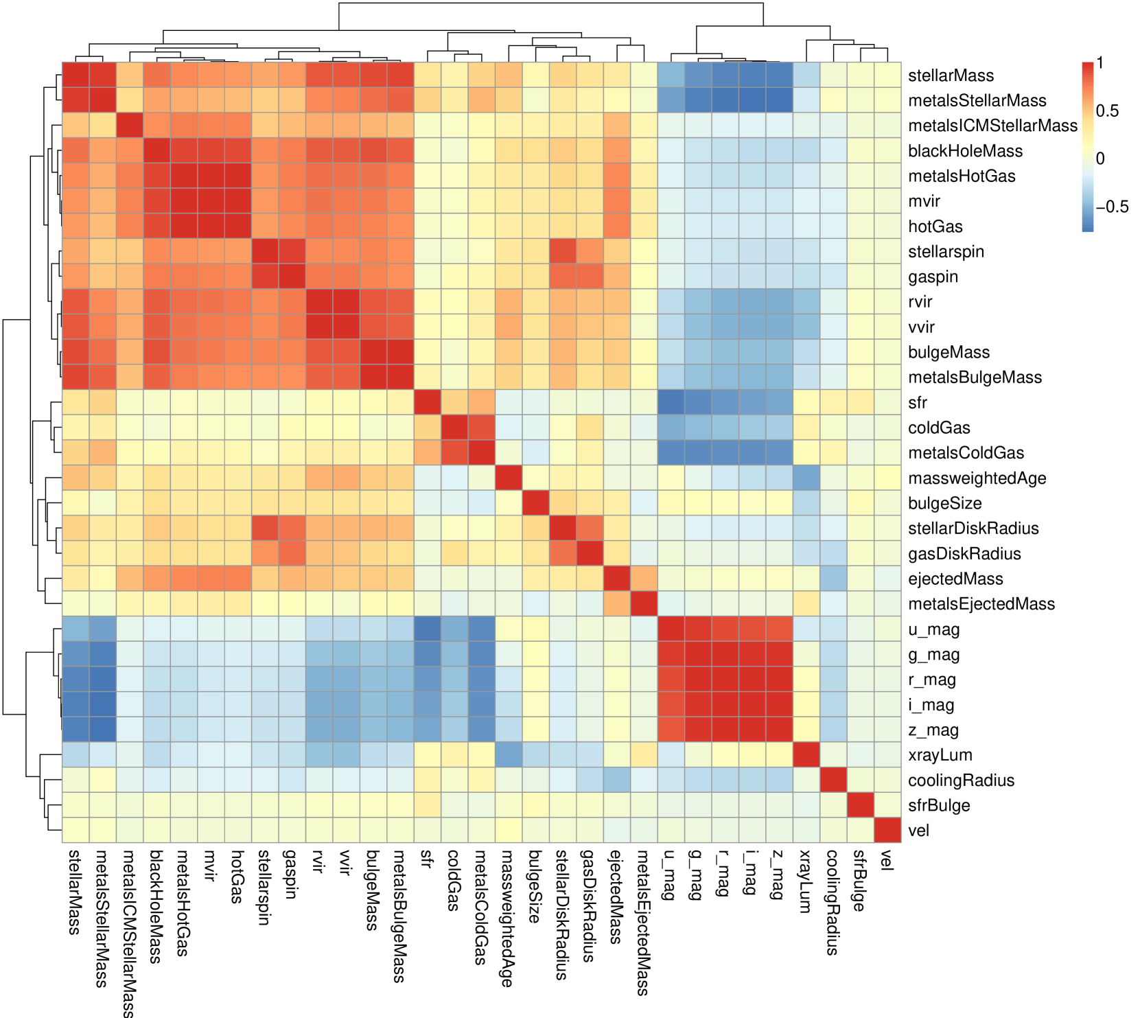
In case of a correlation matrix, the color assigned to a point in the heatmap grid indicates how much each pair of variables correlates, as can be seen in the typical heatmap shown in Fig. 2. For visualization purposes, the arrangement of the rows and columns is made following a hierarchical clustering with a dendrogram drawn at the edges of the matrix. The figure portrays the heatmap of the mock galaxy catalog from Guo et al. (2011). Note the red square in the bottom right corner of the panel, automatically highlighting the trivial association between the magnitudes in the $u,g,r,i$, and $z$ bands. Less trivial associations can be identified more easily using for instance a dendrogram visualization, as discussed in the following section.

Figure 2: Heatmap visualization of the correlation matrix (using a Pearson correlation measure) of some galaxy properties from the mock galaxy catalog by Guo et al. (2011). Red indicates strong positive correlation and blue indicates strong negative correlation. Yellows are associated to correlations close to zero.

4.2 Dendrogram

A dendrogram provides a comprehensive description of the hierarchical structures in a visual format. Among the applications in astronomical research are the hierarchical structural analysis of interstellar properties (Houlahan and Scalo, 1992), molecular clouds (Rosolowsky et al., 2008), and explanatory classification of galaxies (Fraix-Burnet et al., 2012). The individual variables are arranged along the bottom of the dendrogram and referred to as leaf nodes. Clusters are formed by joining individual variables or existing clusters, with the joint point referred to as a node. At each dendrogram node we have a right and left sub-branch of clustered variables. The height of the node can be understood as the dissimilarity $\mathcal{D}$ between the right and left sub-branch clusters.

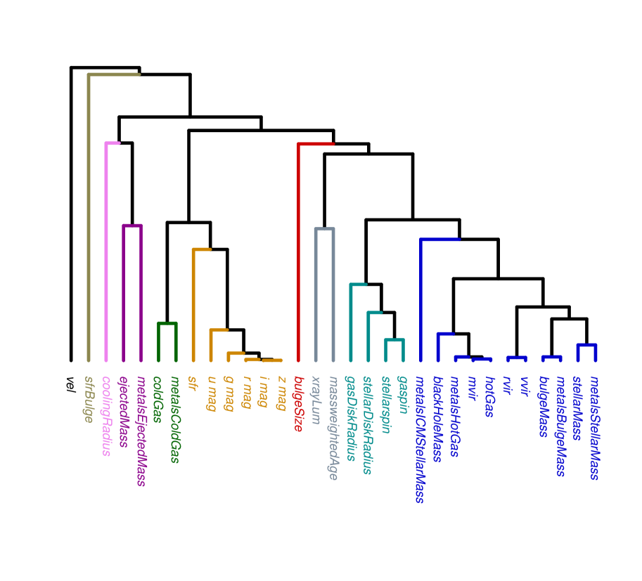
Fig. 3 displays a dendrogram of the galaxy properties from the Guo et al. (2011) catalog, divided in 10 major clusters (indicated by different colors) using the Caliński and Harabasz index. The method automatically suggests interesting associations among the galaxy properties, such as the $u$-band as an indicator of the star formation rate (SFR; see e.g. Gilbank et al., 2010).

Figure 3: Dendrogram of the galaxy properties from the Guo et al. (2011) catalog. The different sub-groups of galaxy properties, assigned using the Caliński and Harabasz index, are colored according to the cluster assignment.

4.3 Graphs

Graphs are powerful tools to represent multivariate data and their relationships. Examples of scientific applications are the analysis of cellular networks (Aittokallio and Schwikowski, 2006), protein interactions (e.g., Fig. 1 from Aragues et al., 2006), and brain disorders (Fig. 2 from Fornito et al., 2015). A graph is defined by a set of vertices representing the objects of study, and a set of edges representing the relationships between them. There are many criteria for judging an optimally drawn graph such as:

• edge crossings should be minimized;

• the vertices should be evenly distributed in the plane;

• the graph should reflect intrinsic symmetries;

• the edges should not cross nodes.

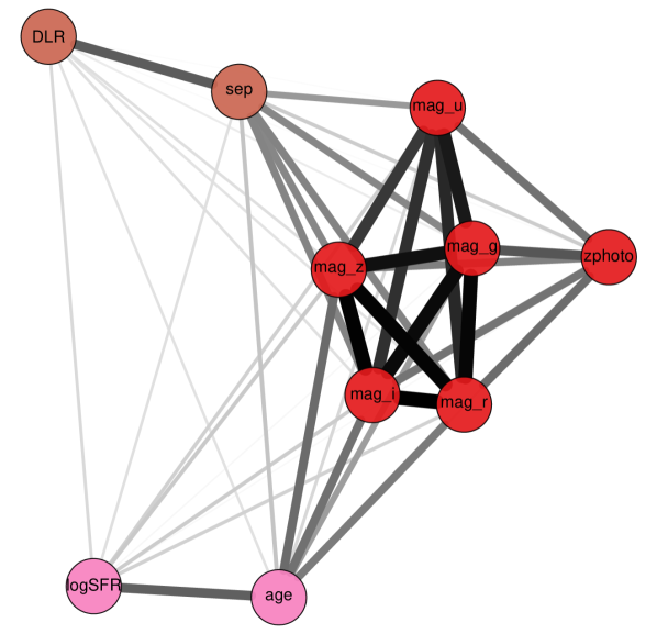
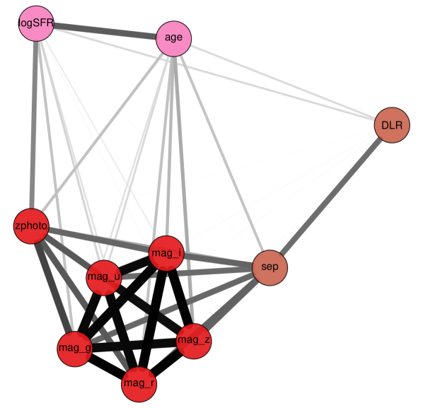
Each item above can be understood as an optimization problem, which is the subject of interest of a research field known as graph drawing (e.g., Tamassia, 2007). There are several methods for graph representations. In this work we use the so-called spring-embedder algorithm (Eades, 1984; Fruchterman and Reingold, 1991). The underlying idea is to allow the vertices to behave like particles moving under the influence of repulsive and attractive forces until the system reaches equilibrium. This graph-drawing algorithm is particularly useful for graphs where the directions of the edges are not important, which is the case of a correlation matrix representation. Fig. 4 displays the correlations among properties of galaxies hosting Type Ia (left) and Type II (right) supernova. Each vertex represents a galaxy property, while the thickness of the edges are weighted by the degree of correlation between each pair of variables (Epskamp et al., 2012). More specifically, the width and color of the edges correspond to the absolute value of the correlations: the higher the correlation, the thicker and more saturated the edge is. Highly correlated parameters appear closer in the graph.

Figure 4: Graph representation of the host galaxy properties from Sako et al. (2014). The thickness of the edges are weighted by the degree of correlation between each pair of variables. The width and color correspond to the degree of association: the higher the correlation, the thicker and more color saturated the edge is. The left (right) side represents the properties of Type Ia (Type II) supernova host galaxies.

4.4 Chord diagram

Chord diagram is a flexible and popular tool that has been used in many different applications, such as identification of relevant signatures in cancer genome (Fig. 1 from Bunting and Nussenzweig, 2013), or study of the relation between foragers and farmers in Central Europe during the Stone Age (Fig. S5 from Bollongino et al., 2013).

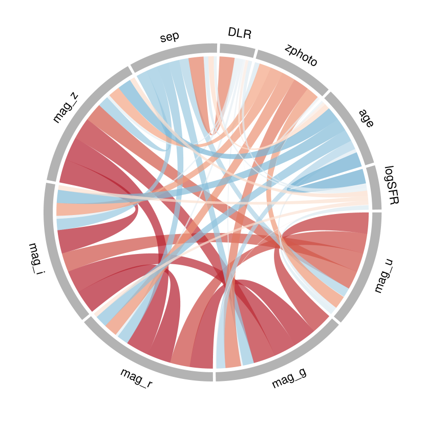
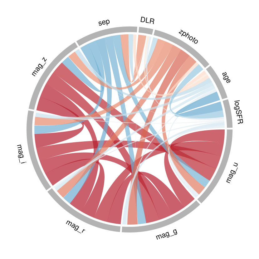
In the case studied here, the chord diagram represents another visualization of the correlation matrix, likewise the graph, heatmap and dendrogram. This tool illustrates relationships between distinct parameters. The columns and rows are represented by segments around the circle. Individual cells are shown as ribbons, which connect the corresponding row and column segments (Gu et al., 2014). The thickness of the ribbons is weighted by the degree of correlation between each pair of variables. Fig. 5 portrays the correlations among supernova Type Ia/II host galaxy properties. For a given choice of colour palette, the colour intensity ranges from fully anti-correlated to correlated values.

Figure 5: A chord diagram representing the Pearson correlations among the galaxy properties hosting Type Ia (left panel), and Type II supernovae (right panel).

4.5 Nightingale chart

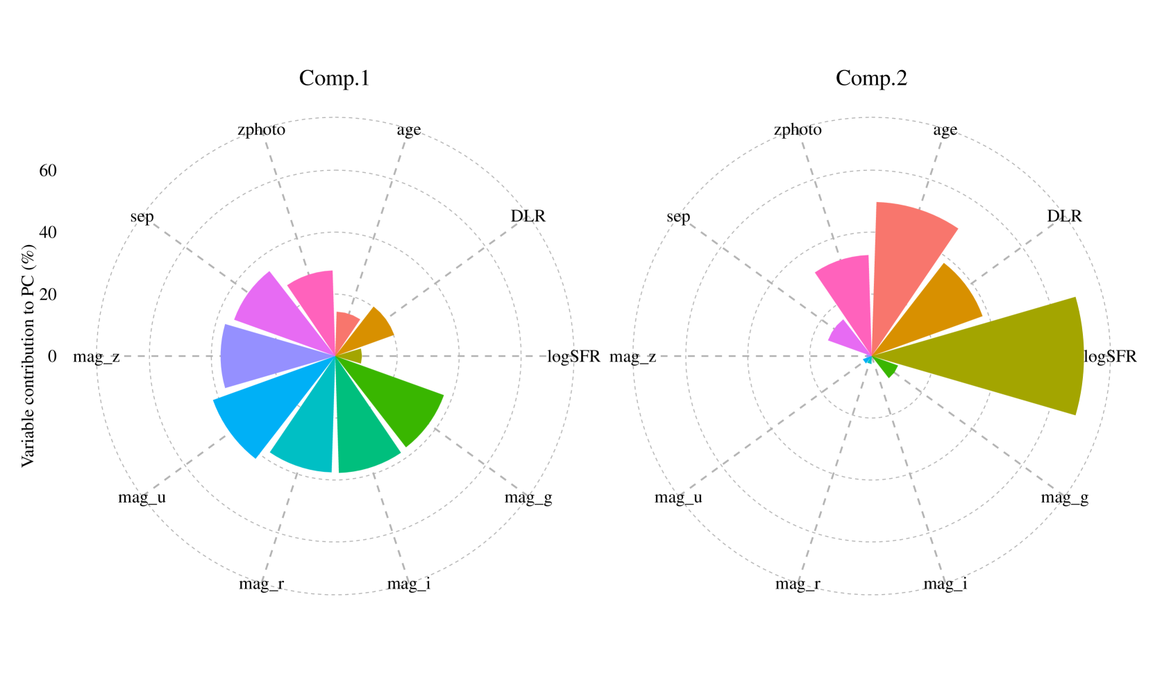
The last plot is inspired by the original Nightingale chart (e.g., Cohen, 1984; McDonald, 2001). This is one of the most influential statistical visualizations of all time, used by Florence Nightingale to convince Queen Victoria about improving hygiene in military hospitals (see also Draper et al., 2009, for a review of radial methods in information visualization).

We show it as a polar bar plot, where the length of each slice represents the relative contribution of each variable to the $i$-th Principal Component. Fig 6 displays the contributions of the supernova Type Ia/II host galaxy properties for the first and second principal components.

Figure 6: A Nightingale diagram representing the contributions of the galaxy properties hosting Type Ia (left panel) and Type II (right panel) supernovae.

5 Summary

We have presented the AMADA package, a web application for interactive exploration and information retrieval of high-dimensional datasets. This is designed for high-dimensional catalogs, with a wide range of applications. There are, though, some limitations in terms of data-size and performance. In particular, shiny allows to upload in the application only up to 1GB of data. Thus, the shiny server should be mostly used for a quick exploration of the package features, so that the user can skip the installation step to familiarize with the code, while we recommend to run AMADA locally (as explained in A) when applied to a real scientific problem. In addition, the speed performance of some methods, such as the hierarchical clustering, may not scale well with very large datasets. As a reference, the processing time to produce a dendrogram from a matrix with 100,000 objects and 100 columns was $\sim 1.5$ seconds on an iMac featuring a 3,5 GHz Intel Core i7 and 32 GB of ram memory. An example of the script to reproduce this test is given below,

⬇

1require(AMADA)

2N = 100000#Number of rows

3M= 100# Number of columns

4M1<-matrix(rnorm(N*M,mean=0,sd=1), N, M)

5ptm <- proc.time()

6corr<-Corr_MIC(M1,"pearson")

7Fig1<-plotdendrogram(corr,"fan")

8proc.time() - ptm

Therefore, despite some limitations, we expect the current version of the package to be suitable for a wide variety of astronomical catalogs. Since this is a software release paper, we avoided a detailed scientific discussion on the available datasets, which here have been used merely as a proof of concept. However, it is worth mentioning that AMADA automatically recovers and displays trivial and non-trivial correlations. An example of the former is the correlation between the u, g, r, z and i magnitudes of supernova host galaxies as seen in Fig. 4, while an example of the latter is the association between the star formation rate and u-band magnitude in the galaxy mock catalog as shown in Fig. 3. It is important to mention that few methods herein implemented are a later development of a previous work from the authors making use of MIC statistics and robust PCA to understand the redshift dependence of halo baryonic properties in the early Universe (de Souza et al., 2014). We therefore refer the reader to this work as an example of application in a cosmological context of the methods discussed here.

The code is freely available on github and can be run both online and locally. This work is part of a larger enterprise known as Cosmostatistics Initiative (COIN), whose philosophy is to enable astronomers to easily introduce novel techniques into their daily research. This is an open-source project, and we expect to continuously add extra features. Therefore, we encourage the users to contact the authors with suggestions, while potential contributors and developers can fork the AMADA repository on github.

Appendix A Running AMADA locally

A.1 From Shiny

To install and run the interface, the first step is to have r in your computer. Thereafter, you have to install the following r packages:

⬇

1install.packages(c("ape","circlize","corrplot","devtools","fpc","ggplot2","ggthemes","MASS","markdown","mclust","minerva","mvtnorm","pcaPP","pheatmap","phytools","qgraph","RColorBrewer","RCurl","squash","stats","shiny"),dependencies=TRUE)

We are now read to install AMADA from GitHub repository:

⬇

1require(devtools)

2install_github("RafaelSdeSouza/AMADA")

An alternative simpler option is to type the following command

⬇

1require(devtools)

2install_github("COINtoolbox/AMADA",dependencies=TRUE)

and r will automatically install the necessary dependencies to run AMADA. After installing the AMADA package, the user can run the visual interface with the following command:

⬇

1require(shiny)

2runUrl("https://github.com/COINtoolbox/AMADA_shiny/archive/master.zip")

AMADA can also be used directly via the web. This option requires no local installation, but the actual processing may be slower. This web interface is hosted by the shinyapps.io platform, and can be accessed directly at http://goo.gl/UTnU7I.

A.2 From R command line

If the user prefer to run AMADA on its own data without relying on the shiny interface, it can be done directly from r command line. An example of how to produce a dendrogram of the Type Ia supernova dataset and saving it as a pdf file is presented below:

⬇

1require(AMADA) #Load the package

2data("SNIa") #Load the SNIa data

3corr<-Corr_MIC(SNIa,"pearson")

4Fig1<-plotdendrogram(corr,"phylogram")

To save the figure as pdf file, with a customized height and width, just type the following:

⬇

1pdf("phylogram.pdf",height = 8,width=8)

2Fig1

3dev.off()

Examples of how the use the other functions inside r can be found in the description file, which can be access via the command

⬇

1help(package="AMADA")

In the current package version, the layout of the figures is mostly hardcoded, but it can be easily changed inside the source code. We expect to add more flexibility in future versions.

References

-
Aittokallio and Schwikowski (2006)
Aittokallio, T., Schwikowski, B., 2006. Graph-based methods for analysing
networks in cell biology. Briefings in Bioinformatics 7 (3), 243–255.
URL http://bib.oxfordjournals.org/content/7/3/243.abstract - Antonuccio-Delogu et al. (2010) Antonuccio-Delogu, V., Dobrotka, A., Becciani, U., Cielo, S., Giocoli, C., Macciò, A. V., Romeo-Veloná, A., Sep. 2010. Dissecting the spin distribution of dark matter haloes. MNRAS407, 1338–1346.
Aragues et al. (2006)
Aragues, R., Jaeggi, D., Oliva, B., 2006. Piana: protein interactions and
network analysis. Bioinformatics 22 (8), 1015–1017.
URL http://bioinformatics.oxfordjournals.org/content/22/8/1015.abstract - Ball and Brunner (2010) Ball, N. M., Brunner, R. J., 2010. Data Mining and Machine Learning in Astronomy. International Journal of Modern Physics D 19, 1049–1106.
Bollongino et al. (2013)
Bollongino, R., Nehlich, O., Richards, M. P., Orschiedt, J., Thomas,
M. G., Sell, C., Fajkosová, Z., Powell, A., Burger, J., 2013. 2000
years of parallel societies in stone age central europe. Science 342 (6157),
479–481.
URL http://www.sciencemag.org/content/342/6157/479.abstract - Borne et al. (2008) Borne, K., Becla, J., Davidson, I., Szalay, A., Tyson, J. A., Dec. 2008. The LSST Data Mining Research Agenda. In: Bailer-Jones, C. A. L. (Ed.), American Institute of Physics Conference Series. Vol. 1082 of American Institute of Physics Conference Series. pp. 347–351.
- Brescia et al. (2010) Brescia, M., Longo, G., Djorgovski, G. S., Cavuoti, S., D’Abrusco, R., Donalek, C., Di Guido, A., Fiore, M., Garofalo, M., Laurino, O., Mahabal, A., Manna, F., Nocella, A., d’Angelo, G., Paolillo, M., Oct. 2010. DAME: A Web Oriented Infrastructure for Scientific Data Mining & Exploration. ArXiv e-prints.
Bunting and Nussenzweig (2013)
Bunting, S. F., Nussenzweig, A., Jul. 2013. End-joining, translocations and
cancer. Nat Rev Cancer 13 (7), 443–454.
URL http://dx.doi.org/10.1038/nrc3537 - Burger et al. (2013) Burger, D., Stassun, K. G., Pepper, J., Siverd, R. J., Paegert, M., De Lee, N. M., Robinson, W. H., Aug. 2013. Filtergraph: An interactive web application for visualization of astronomy datasets. Astronomy and Computing 2, 40–45.
- Burgess et al. (2014) Burgess, J. M., Preece, R. D., Ryde, F., Veres, P., Mészáros, P., Connaughton, V., Briggs, M., Pe’er, A., Iyyani, S., et a., Apr. 2014. An Observed Correlation between Thermal and Non-thermal Emission in Gamma-Ray Bursts. ApJ784, L43.
Caliński and Harabasz (1974)
Caliński, T., Harabasz, J., 1974. A dendrite method for cluster analysis.
Communications in Statistics 3 (1), 1–27.
URL http://www.tandfonline.com/doi/abs/10.1080/03610927408827101 - Carilli (2014) Carilli, C. L., Aug. 2014. Square Kilometre Array key science: a progressive retrospective. ArXiv e-prints.
- Chakraborty et al. (2013) Chakraborty, A., Feigelson, E. D., Babu, G. J., Mar. 2013. VOStat: A Statistical Web Service for Astronomers. PASP125, 295–305.
- Chen et al. (2009) Chen, Y.-M., Wild, V., Kauffmann, G., Blaizot, J., Davis, M., Noeske, K., Wang, J.-M., Willmer, C., Feb. 2009. Constraints on the star formation histories of galaxies from z ~ 1 to 0. MNRAS393, 406–418.
Cohen (1984)
Cohen, I. B., Mar. 1984. Florence nightingale 250 (3), 128–137.
URL http://www.nature.com/scientificamerican/journal/v250/n3/pdf/scientificamerican0384-128.pdf - Conselice (2006) Conselice, C. J., Dec. 2006. The fundamental properties of galaxies and a new galaxy classification system. MNRAS373, 1389–1408.
- Croux et al. (2007) Croux, C., Filzmoser, P., Oliveira, M., Mar. 2007. Algorithms for Projection?Pursuit robust principal component analysis. Chemometrics and Intelligent Laboratory Systems 87 (2), 218.
- de Souza et al. (2015) de Souza, R. S., Cameron, E., Killedar, M., Hilbe, J., Vilalta, R., Maio, U., Biffi, V., Ciardi, B., Riggs, J. D., Sep. 2015. The Overlooked Potential of Generalized Linear Models in Astronomy - I: Binomial Regression and Numerical Simulations. arXiv:1409.7696.
- de Souza et al. (2013a) de Souza, R. S., Ciardi, B., Maio, U., Ferrara, A., Jan. 2013a. Dark matter halo environment for primordial star formation. MNRAS428, 2109–2117.
- de Souza et al. (2013b) de Souza, R. S., Ishida, E. E. O., Johnson, J. L., Whalen, D. J., Mesinger, A., Dec. 2013b. Detectability of the first cosmic explosions. MNRAS436, 1555–1563.
- de Souza et al. (2014b) de Souza, R. S., Ishida, E. E. O., Whalen, D. J., Johnson, J. L., Ferrara, A., Aug. 2014b. Probing the stellar initial mass function with high-z supernovae. MNRAS442, 1640–1655.
- de Souza et al. (2014) de Souza, R. S., Maio, U., Biffi, V., Ciardi, B., May 2014. Robust PCA and MIC statistics of baryons in early minihaloes. MNRAS440, 240–248.
- de Souza et al. (2014a) de Souza, R. S., Maio, U., Biffi, V., Ciardi, B., May 2014a. Robust PCA and MIC statistics of baryons in early minihaloes. MNRAS440, 240–248.
- Donalek et al. (2013) Donalek, C., Djorgovski, S., Mahabal, A., Graham, M., Drake, A., Fuchs, T., Turmon, M., Arun Kumar, A., Philip, N., Yang, M.-C., Longo, G., Oct 2013. Feature selection strategies for classifying high dimensional astronomical data sets. In: Big Data, 2013 IEEE International Conference on. pp. 35–41.
- Draper et al. (2009) Draper, G., Livnat, Y., Riesenfeld, R., Sept 2009. A survey of radial methods for information visualization. Visualization and Computer Graphics, IEEE Transactions on 15 (5), 759–776.
- Eades (1984) Eades, P., 1984. A heuristic for graph drawing. Congressus Numerantium 42, 149–160.
Epskamp et al. (2012)
Epskamp, S., Cramer, A. O., Waldorp, L. J., Schmittmann, V. D., Borsboom, D., 5
2012. qgraph: Network visualizations of relationships in psychometric data.
Journal of Statistical Software 48 (4), 1–18.
URL http://www.jstatsoft.org/v48/i04 - Faber and Jackson (1976) Faber, S. M., Jackson, R. E., Mar. 1976. Velocity dispersions and mass-to-light ratios for elliptical galaxies. ApJ204, 668–683.
Fisher (1936)
Fisher, R. A., 1936. The use of multiple measurements in taxonomic problems.
Annals of Eugenics 7 (2), 179–188.
URL http://dx.doi.org/10.1111/j.1469-1809.1936.tb02137.x -
Fornito et al. (2015)
Fornito, A., Zalesky, A., Breakspear, M., Feb. 2015. The connectomics of brain
disorders. Nature Reviews Neuroscience 16 (3), 159–172.
URL http://dx.doi.org/10.1038/nrn3901 - Fraix-Burnet et al. (2012) Fraix-Burnet, D., Chattopadhyay, T., Chattopadhyay, A. K., Davoust, E., Thuillard, M., Sep. 2012. A six-parameter space to describe galaxy diversification. A&A545, A80.
Fruchterman and Reingold (1991)
Fruchterman, T. M. J., Reingold, E. M., 1991. Graph drawing by force-directed
placement. Softw., Pract. Exper. 21 (11), 1129–1164.
URL http://dblp.uni-trier.de/db/journals/spe/spe21.html#FruchtermanR91 - Gilbank et al. (2010) Gilbank, D. G., Baldry, I. K., Balogh, M. L., Glazebrook, K., Bower, R. G., Jul. 2010. The local star formation rate density: assessing calibrations using [OII], H and UV luminosities. MNRAS405, 2594–2614.
- Graham et al. (2013) Graham, M. J., Djorgovski, S. G., Mahabal, A. A., Donalek, C., Drake, A. J., May 2013. Machine-assisted discovery of relationships in astronomy. MNRAS431, 2371–2384.
Gu et al. (2014)
Gu, Z., Gu, L., Eils, R., Schlesner, M., Brors, B., 2014. circlize implements
and enhances circular visualization in r. Bioinformatics.
URL http://bioinformatics.oxfordjournals.org/content/early/2014/06/14/bioinformatics.btu393.abstract - Guo et al. (2011) Guo, Q., White, S., Boylan-Kolchin, M., De Lucia, G., Kauffmann, G., Lemson, G., Li, C., Springel, V., Weinmann, S., May 2011. From dwarf spheroidals to cD galaxies: simulating the galaxy population in a CDM cosmology. MNRAS413, 101–131.
- Hamaus et al. (2014) Hamaus, N., Wandelt, B. D., Sutter, P. M., Lavaux, G., Warren, M. S., Jan. 2014. Cosmology with Void-Galaxy Correlations. Physical Review Letters 112 (4), 041304.
Hampel et al. (2005)
Hampel, F. R., Ronchetti, E. M., Rousseeuw, P. J., Stahel, W. A., 2005. Front
Matter. John Wiley & Sons, Inc.
URL http://dx.doi.org/10.1002/9781118186435.fmatter - Hoaglin et al. (2000) Hoaglin, D. C., Mosteller, F., (Editor), J. W. T., 2000. Understanding Robust and Exploratory Data Analysis, 1st Edition. Wiley-Interscience.
- Houlahan and Scalo (1992) Houlahan, P., Scalo, J., Jul. 1992. Recognition and characterization of hierarchical interstellar structure. II - Structure tree statistics. ApJ393, 172–187.
Howell (2005)
Howell, D. C., 2005. Median Absolute Deviation. John Wiley & Sons, Ltd.
URL http://dx.doi.org/10.1002/0470013192.bsa384 - Ishida and de Souza (2011) Ishida, E. E. O., de Souza, R. S., Mar. 2011. Hubble parameter reconstruction from a principal component analysis: minimizing the bias. A&A527, A49.
- Ishida and de Souza (2013) Ishida, E. E. O., de Souza, R. S., Mar. 2013. Kernel PCA for Type Ia supernovae photometric classification. MNRAS430, 509–532.
- Ishida et al. (2011) Ishida, E. E. O., de Souza, R. S., Ferrara, A., Nov. 2011. Probing cosmic star formation up to z= 9.4 with gamma-ray bursts. MNRAS418, 500–504.
- Kembhavi et al. (2015) Kembhavi, A. K., Mahabal, A. A., Kale, T., Jagade, S., Vibhute, A., Garg, P., Vaghmare, K., Navelkar, S., Agrawal, T., Nandrekar, D., Shaikh, M., Mar. 2015. AstroStat - A VO Tool for Statistical Analysis. arxiv:1503.02989.
- Konstantopoulos (2015) Konstantopoulos, I. S., Apr. 2015. The starfish diagram: Visualising data within the context of survey samples. Astronomy and Computing 10, 116–120.
- Lee et al. (2013) Lee, B., Giavalisco, M., Williams, C. C., Guo, Y., Lotz, J., Van der Wel, A., Ferguson, H. C., Faber, S. M., Koekemoer, A., Grogin, N., Kocevski, D., Conselice, C. J., Wuyts, S., Dekel, A., Kartaltepe, J., Bell, E. F., Sep. 2013. CANDELS: The Correlation between Galaxy Morphology and Star Formation Activity at z ~ 2. ApJ774, 47.
Li (1990)
Li, W., 1990. Mutual information functions versus correlation functions.
Journal of Statistical Physics 60 (5-6), 823–837.
URL http://dx.doi.org/10.1007/BF01025996 - LSST Science Collaboration et al. (2009) LSST Science Collaboration, Abell, P. A., Allison, J., Anderson, S. F., Andrew, J. R., Angel, J. R. P., Armus, L., Arnett, D., Asztalos, S. J., Axelrod, T. S., et al., Dec. 2009. LSST Science Book, Version 2.0. arXiv:0912.0201.
- Martinez-Gomez et al. (2013) Martinez-Gomez, E., Richards, M. T., Richards, D. S. P., Aug. 2013. Distance Correlation Methods for Discovering Associations in Large Astrophysical Databases. arxiv:1308.3925.
McDonald (2001)
McDonald, L., 2001. Florence nightingale and the early origins of
evidence-based nursing. Evidence Based Nursing 4 (3), 68–69.
URL http://ebn.bmj.com/content/4/3/68.short - McGurk et al. (2010) McGurk, R. C., Kimball, A. E., Ivezić, Ž., Mar. 2010. Principal Component Analysis of Sloan Digital Sky Survey Stellar Spectra. AJ139, 1261–1268.
- Overzier et al. (2013) Overzier, R., Lemson, G., Angulo, R. E., Bertin, E., Blaizot, J., Henriques, B. M. B., Marleau, G.-D., White, S. D. M., Jan. 2013. The Millennium Run Observatory: first light. MNRAS428, 778–803.
Paradis et al. (2004)
Paradis, E., Claude, J., Strimmer, K., 2004. Ape: Analyses of phylogenetics and
evolution in r language. Bioinformatics 20 (2), 289–290.
URL http://bioinformatics.oxfordjournals.org/content/20/2/289 -
Patty and Penn (2015)
Patty, J. W., Penn, E. M., 1 2015. Analyzing big data: Social choice and
measurement. PS: Political Science & Politics 48, 95–101.
URL http://journals.cambridge.org/article_S1049096514001814 -
Pearson (1895)
Pearson, K., 1895. Note on regression and inheritance in the case of two
parents. Proceedings of the Royal Society of London 58 (347-352), 240–242.
URL http://rspl.royalsocietypublishing.org/content/58/347-352/240.short - Reshef et al. (2011) Reshef, D. N., Reshef, Y. A., Finucane, H. K., Grossman, S. R., McVean, G., Turnbaugh, P. J., Lander, E. S., Mitzenmacher, M., Sabeti, P. C., Dec. 2011. Detecting Novel Associations in Large Data Sets. Science 334, 1518–.
- Rosolowsky et al. (2008) Rosolowsky, E. W., Pineda, J. E., Kauffmann, J., Goodman, A. A., Jun. 2008. Structural Analysis of Molecular Clouds: Dendrograms. ApJ679, 1338–1351.
- Sako et al. (2014) Sako, M., Bassett, B., Becker, A. C., Brown, P. J., Campbell, H., Cane, R., Cinabro, D., D’Andrea, C. B., et al., Jan. 2014. The Data Release of the Sloan Digital Sky Survey-II Supernova Survey. arxiv:1401.3317.
- Scaramella et al. (2015) Scaramella, R., Mellier, Y., Amiaux, J., Burigana, C., Carvalho, C. S., Cuillandre, J. C., da Silva, A., Dinis, J., Derosa, A., Maiorano, E., Franzetti, P., Garilli, B., Maris, M., Meneghetti, M., Tereno, I., Wachter, S., Amendola, L., Cropper, M., Cardone, V., Massey, R., Niemi, S., Hoekstra, H., Kitching, T., Miller, L., Schrabback, T., Semboloni, E., Taylor, A., Viola, M., Maciaszek, T., Ealet, A., Guzzo, L., Jahnke, K., Percival, W., Pasian, F., Sauvage, M., the Euclid Collaboration, Jan. 2015. Euclid space mission: a cosmological challenge for the next 15 years. ArXiv e-prints.
- Scarlata et al. (2007) Scarlata, C., Carollo, C. M., Lilly, S., Sargent, M. T., Feldmann, R., Kampczyk, P., Porciani, C., Koekemoer, A., et al., Sep. 2007. COSMOS Morphological Classification with the Zurich Estimator of Structural Types (ZEST) and the Evolution Since z = 1 of the Luminosity Function of Early, Disk, and Irregular Galaxies. ApJS172, 406–433.
- Schuh et al. (2015) Schuh, M. A., Banda, J. M., Wylie, T., McInerney, P., Pillai, K. G., Angryk, R. A., Apr. 2015. On visualization techniques for solar data mining. Astronomy and Computing 10, 32–42.
Spearman (1904)
Spearman, C., 1904. The proof and measurement of association between two
things. The American Journal of Psychology 15 (1), pp. 72–101.
URL http://www.jstor.org/stable/1412159 - Springel (2005) Springel, V., Dec. 2005. The cosmological simulation code GADGET-2. MNRAS364, 1105–1134.
- Tamassia (2007) Tamassia, R., 2007. Handbook of Graph Drawing and Visualization (Discrete Mathematics and Its Applications). Chapman & Hall/CRC.
- Tully and Fisher (1977) Tully, R. B., Fisher, J. R., Feb. 1977. A new method of determining distances to galaxies. A&A54, 661–673.
van Zyl (2014)
van Zyl, T., 2015/03/03 2014. Machine Learning on Geospatial Big Data. CRC
Press, pp. 133–148.
URL http://dx.doi.org/10.1201/b16524-8 -
Venter et al. (2004)
Venter, J. C., Remington, K., Heidelberg, J. F., Halpern, A. L., Rusch, D.,
Eisen, J. A., Wu, D., Paulsen, I., Nelson, K. E., Nelson, W., Fouts, D. E.,
Levy, S., Knap, A. H., Lomas, M. W., Nealson, K., White, O., Peterson, J.,
Hoffman, J., Parsons, R., Baden-Tillson, H., Pfannkoch, C., Rogers, Y.-H.,
Smith, H. O., 2004. Environmental genome shotgun sequencing of the sargasso
sea. Science 304 (5667), 66–74.
URL http://www.sciencemag.org/content/304/5667/66.abstract - Vogelsberger et al. (2014) Vogelsberger, M., Genel, S., Springel, V., Torrey, P., Sijacki, D., Xu, D., Snyder, G., Nelson, D., Hernquist, L., Oct. 2014. Introducing the Illustris Project: simulating the coevolution of dark and visible matter in the Universe. MNRAS444, 1518–1547.
Wilkinson and Friendly (2009)
Wilkinson, L., Friendly, M., 2009. The history of the cluster heat map. The
American Statistician 63 (2), 179–184.
URL http://dx.doi.org/10.1198/tas.2009.0033 - Yates et al. (2012) Yates, R. M., Kauffmann, G., Guo, Q., May 2012. The relation between metallicity, stellar mass and star formation in galaxies: an analysis of observational and model data. MNRAS422, 215–231.