Mott physics and spin fluctuations: a unified framework

Abstract

We present a formalism for strongly correlated electrons systems which consists in a local approximation of the dynamical three-leg interaction vertex. This vertex is self-consistently computed with a quantum impurity model with dynamical interactions in the charge and spin channels, similar to dynamical mean field theory (DMFT) approaches. The electronic self-energy and the polarization are both frequency and momentum dependent. The method interpolates between the spin-fluctuation or GW approximations at weak coupling and the atomic limit at strong coupling. We apply the formalism to the Hubbard model on a two-dimensional square lattice and show that as interactions are increased towards the Mott insulating state, the local vertex acquires a strong frequency dependence, driving the system to a Mott transition, while at low enough temperatures the momentum-dependence of the self-energy is enhanced due to large spin fluctuations. Upon doping, we find a Fermi arc in the one-particle spectral function, which is one signature of the pseudo-gap state.

Strongly-correlated electronic systems like high-temperature cuprate superconductors are a major challenge in condensed-matter physics.

One theoretical approach to cuprates emphasizes the effect of long-range bosonic fluctuations on the electronic fluid, for example long-range antiferromagnetic (AF) fluctuations due to a quantum critical point Chubukov et al. (2002); Efetov et al. (2013); Wang and Chubukov (2014); Metlitski and Sachdev (2010); Onufrieva and Pfeuty (2009, 2012). These bosonic fluctuations are also central to approaches such as the two-particle self-consistent approximation (TPSC Vilk et al. (1994); Daré et al. (1996); Vilk and Tremblay (1996, 1997); Tremblay (2011)), the GW approximation Hedin (1965) and the fluctuation-exchange approximation (FLEX Bickers and Scalapino (1989)).

Another approach focusses, following Anderson Anderson (1987), on describing the Mott transition and the doped Mott insulator. In recent years, dynamical mean field theory (DMFT) Georges et al. (1996) and its cluster extensions like CDMFT Lichtenstein and Katsnelson (2000); Kotliar et al. (2001) or DCA Hettler et al. (1998, 1999); Maier et al. (2005a) have allowed for tremendous theoretical progress on the Mott transition both for models and realistic computations of strongly correlated materials Kotliar et al. (2006). In particular, numerous works have been devoted to the one-band Hubbard model, mapping out its phase diagram, studying the $d$-wave superconducting order and the pseudogap Kyung et al. (2009); Sordi et al. (2012a); Civelli et al. (2008); Ferrero et al. (2010); Gull et al. (2013); Macridin et al. (2004); Maier et al. (2004, 2005b, 2006); Gull et al. (2010); Yang et al. (2011); Macridin and Jarrell (2008); Macridin et al. (2006); Jarrell et al. (2001); Bergeron et al. (2011); Kyung et al. (2004, 2006); Okamoto et al. (2010); Sordi et al. (2010, 2012b); Civelli et al. (2005); Ferrero et al. (2008, 2009); Gull et al. (2009). Cluster DMFT is one of the few methods designed for the strong-interaction regime to have a simple control parameter, namely the size $N_{c}$ of the cluster or the momentum resolution of the electronic self-energy. It interpolates between the DMFT solution ($N_{c}=1$) and the exact solution of the Hubbard model ($N_{c}=\infty$). Despite its success, this method nonetheless suffers from severe limitations: i) it does not include the effect of long-range bosonic modes of wavelengths larger than the cluster size; ii) the negative sign problem of continuous-time quantum Monte Carlo has so far precluded the convergence of the cluster solutions with respect to $N_{c}$ in the most important regimes like the pseudogap; iii) the $\mathbf{k}$-resolution of the self-energy is still quite coarse in DCA (typically 8 or 16 patches in the Brillouin zone, see e.g. Gull et al. (2009, 2010); Vidhyadhiraja et al. (2009); Macridin and Jarrell (2008)), or relies on uncontrolled a posteriori “periodization” techniques in CDMFT Kotliar et al. (2001).

Several directions beyond cluster DMFT methods are currently under investigation to address these issues, such as GW + DMFT Sun and Kotliar (2002, 2004); Biermann et al. (2003); Ayral et al. (2012, 2013); Hansmann et al. (2013); Huang et al. (2014), the $\mathrm{D\Gamma A}$ method Toschi et al. (2007); Katanin et al. (2009); Schäfer et al. (2015); Valli et al. (2014), the dual fermion Rubtsov et al. (2008) and dual boson methods Rubtsov et al. (2012); Hafermann et al. (2014), or combinations of DMFT with functional renormalization group methods Taranto et al. (2014).

In this letter, we discuss a simple formalism that unifies the two points of view mentioned above. It is designed to encompass both Mott physics à la DMFT and the effect of medium and long-range bosonic modes. It interpolates between the atomic limit in the strong-interaction regime and the “fluctuation-exchange” limit in the weak-interaction regime. It consists in decoupling the electron-electron interaction term by Hubbard-Stratonovich bosonic fields and making a local self-consistent approximation of the lattice’s electron-boson one-particle irreducible vertex, using a quantum impurity model similar to the one used in DMFT. It can be formally derived from a functional of the vertex given by three-particle irreducible diagrams Dominicis and Martin (1964a, b). In the following, we will therefore denote this method as a triply-irreducible local expansion, or TRILEX. Already at the single-site level, it produces, in some parameter regimes, a momentum-dependent self-energy and polarization, at a small computational cost, similar to solving Extended DMFT (EDMFT) Sengupta and Georges (1995); Kajueter (1996); Si and Smith (1996). In the following, we first introduce the method; we then present the solution of the single-site version of TRILEX for the two-dimensional Hubbard model.

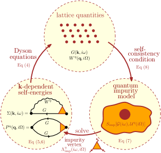
Figure 1: (color online) Description of the TRILEX method

We focus on the Hubbard model defined by the following Hamiltonian:

$$H=\sum_{ij}t_{ij}c_{i}^{\dagger}c_{j}+U\sum_{i}n_{i\uparrow}n_{i\downarrow}$$ (1)

The indices $i,j$ denote lattice sites, $\sigma=\uparrow,\downarrow$, $c_{i\sigma}^{\dagger}$ and $c_{i\sigma}$ are fermionic creation and annihilation operators, and $n_{i\sigma}\equiv c_{i\sigma}^{\dagger}c_{i\sigma}$. $t_{ij}$ is the tight-binding hopping matrix $(t_{ij}=t(t^{\prime})$ for (next-)nearest-neighbors), while $U$ is the on-site Coulomb interaction. We rewrite the operators of the interaction term as:

$$Un_{i\uparrow}n_{i\downarrow}=\frac{1}{2}\sum_{I}U^{I}n_{i}^{I}n_{i}^{I}$$ (2)

where $U^{I}$ is the bare interaction in channel $I$, and $n_{i}^{I}\equiv\sum_{\sigma\sigma^{\prime}}c_{i\sigma}^{*}\sigma_{\sigma\sigma^{\prime}}^{I}c_{i\sigma^{\prime}}$ where $\sigma^{0}=\mathbf{1}$ and $\sigma^{x,y,z}$ are the Pauli matrices. In this paper, we consider two decouplings: (a) in the charge and vector spin channel ($I=0,x,y,z$) (“$xyz$-decoupling”), $U^{x}=U^{y}=U^{z}\equiv U^{\mathrm{sp}}$ and $U^{0}\equiv U^{\mathrm{ch}}$, $U^{\mathrm{sp}}$ and $U^{\mathrm{ch}}$ satisfy: $U=U^{\mathrm{ch}}-3U^{\mathrm{sp}}$; (b) in the charge and longitudinal spin channel only ($I=0,z$) (“$z$-decoupling”), $U=U^{\mathrm{ch}}-U^{\mathrm{sp}}$. In both cases, we have two channels, denoted as $\eta=\mathrm{ch},\mathrm{sp}$. In this paper, we fix the ratio to $U^{\mathrm{ch}}=U/2$ and $U^{\mathrm{sp}}=-U/6$ ($xyz$ decoupling) and $U^{\mathrm{ch}}=U/2$ and $U^{\mathrm{sp}}=-U/2$ ($z$ decoupling). We now decouple (2) using real bosonic Hubbard-Stratonovich fields $\phi_{i}^{I}(\tau)$ in each channel and at each lattice site, so that the action becomes:

$$S_{\mathrm{latt}} = \int_{0}^{\beta}d\tau\sum_{ij}c_{i\sigma\tau}^{*}\left\{\partial_{\tau}+t_{ij}\right\}c_{j\sigma\tau}$$ (3)

$$+\sum_{i,I}\left[\frac{1}{2}(U^{I})^{-1}\phi_{i\tau}^{I}\phi_{i\tau}^{I}+\lambda^{I}\phi_{i\tau}^{I}n_{i\tau}^{I}\right]$$

$c_{i\sigma\tau}^{*}$ and $c_{i\sigma\tau}$ are conjugate $\beta$-antiperiodic Grassmann fields, and $\lambda^{I}=1$. We are now dealing with an interacting lattice problem with a local electron-boson coupling. The lattice Green’s functions $G(\mathbf{k},i\omega)$ and $W^{\eta}(\mathbf{q},i\Omega)$ (the Fourier transforms of $-\langle c_{i\sigma\tau}c_{j\sigma 0}^{*}\rangle$ and $-\langle\phi_{i\sigma\tau}^{\eta}\phi_{j\sigma 0}^{\eta}\rangle$, respectively) are given by Dyson equations:

$$G(\mathbf{k},i\omega) = \left[i\omega+\mu-\epsilon(\mathbf{k})-\Sigma(\mathbf{k},i\omega)\right]^{-1}$$ (4a)

$$W^{\eta}(\mathbf{q},i\Omega) = U^{\eta}\left[1-U^{\eta}P^{\eta}(\mathbf{q},i\Omega)\right]^{-1}$$ (4b)

$\mathbf{k}$ and $\mathbf{q}$ are momentum variables, $i\omega$($i\Omega$) stands for a fermionic (bosonic) Matsubara frequency, $\epsilon(\mathbf{k})$ is the Fourier transform of $t_{ij}$, and $\mu$ is the chemical potential. The fermionic and bosonic self-energies $\Sigma$ and $P^{\eta}$ are given by the exact expressions (written here for the paramagnetic normal phase) (see e.g Aryasetiawan and Biermann (2008)):

$$\Sigma(\mathbf{k},i\omega) = -\sum_{\begin{subarray}{c}\mathbf{q},i\Omega,\\ \eta=\mathrm{ch},\mathrm{sp}\end{subarray}}m_{\eta}\lambda^{\eta}G_{\begin{subarray}{c}\mathbf{q+k},\\ i\omega+i\Omega\end{subarray}}W_{\mathbf{q},i\Omega}^{\eta}\Lambda_{\begin{subarray}{c}\mathbf{k},\mathbf{q},\\ i\omega,i\Omega\end{subarray}}^{\eta}$$ (5a)

$$P^{\eta}(\mathbf{q},i\Omega) = 2\sum_{\mathbf{k},i\omega}\lambda^{\eta}G_{\begin{subarray}{c}\mathbf{q+k},\\ i\omega+i\Omega\end{subarray}}G_{\mathbf{k},i\omega}\Lambda_{\begin{subarray}{c}\mathbf{k},\mathbf{q},\\ i\omega,i\Omega\end{subarray}}^{\eta}$$ (5b)

Here, $m_{\mathrm{ch}}=1$, $m_{\mathrm{sp}}=3$ ($xyz$ decoupling) or $m_{\mathrm{sp}}=1$ ($z$ decoupling). $\Lambda^{\eta}(\mathbf{q},\mathbf{k},i\omega,i\Omega)$ is the exact one-particle irreducible electron-boson coupling (or Hedin) vertex, namely the effective interaction between electrons and bosons renormalized by electronic interactions.

The main point of this paper consists in approximating the vertex $\Lambda^{\eta}(\mathbf{q},\mathbf{k},i\omega,i\Omega)$ by the local, but two-frequency-dependent $\Lambda_{\mathrm{imp}}^{\eta}(i\omega,i\Omega)$ computed from a self-consistent quantum impurity problem:

$$\Lambda^{\eta}(\mathbf{q},\mathbf{k},i\omega,i\Omega)\approx\Lambda_{\mathrm{imp}}^{\eta}(i\omega,i\Omega)$$ (6)

This strategy radically differs from DMFT, EDMFT and GW+DMFT which approximate the self-energy $\Sigma$ (and $P$), not $\Lambda$. It implies that our $\Sigma$ and $P$ (computed from (5a-5b)) are, in some parameter regimes, strongly momentum-dependent while containing local vertex corrections which will be essential to capture Mott physics (see also Ayral et al. (2012)). Formally, DMFT is a local approximation of the two-particle irreducible Luttinger-Ward functional $\Phi_{\mathrm{LW}}[G]$ Georges and Kotliar (1992); Georges et al. (1996). In contrast, our approximation can be defined as a local approximation of the three-particle irreducible functional $\mathcal{K}[G,W,\Lambda]$ introduced in Dominicis and Martin (1964a, b) as a generalization of $\Phi_{\mathrm{LW}}$ to higher degrees of irreducibility. We therefore denote it as TRILEX, triply-irreducible local expansion. It makes it exact in the limit of infinite dimensions. The formal derivation of the method will be provided elsewhere Ayral and Parcollet .

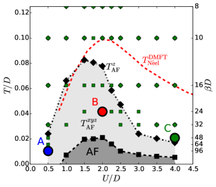
Figure 2: (color online) $(T,U$) Phase diagram (half-filling, $t^{\prime}=0$). The black diamonds (resp. squares) denote $T_{\mathrm{AF}}^{z}$ (resp. $T_{\mathrm{AF}}^{xyz}$); the dashed lines are guides to the eye. The green diamonds (resp. squares) denote converged TRILEX solutions in the $z$ (resp. $x,y,z$) decoupling. A, B, and C are defined as A: $\beta D=96$, $U/D=0.5$, B: $\beta D=24$, $U/D=2$, C: $\beta D=48$, $U/D=4$. The red dotted line denotes $T_{\mathrm{N\acute{e}el}}^{DMFT}$ for the square lattice (from Kuneš (2011)).

The action of the impurity model reads:

$$S_{\mathrm{imp}} = -\iint_{0}^{\beta}d\tau d\tau^{\prime}\sum_{\sigma}c_{\sigma\tau}^{*}\mathcal{G}(\tau-\tau^{\prime})c_{\sigma\tau^{\prime}}$$ (7)

$$+\frac{1}{2}\sum_{I}\iint_{0}^{\beta}d\tau d\tau^{\prime}n_{\tau}^{I}\mathcal{U}^{I}(\tau-\tau^{\prime})n_{\tau^{\prime}}^{I}$$

This is an Anderson quantum impurity with retarded charge-charge ($I=0$) and spin-spin ($I=x,y,z$ in the $xyz$-decoupling, $I=z$ in the $z$-decoupling) interactions. The bosonic fields $\phi^{I}$ have been integrated out to obtain a fermionic action with retarded interactions amenable to numerical computations. We compute the fermionic three-point correlation functions to reconstruct the electron-boson vertex $\Lambda_{\mathrm{imp}}$ (as shown in the Suppl. Mat., section B). Finally, $\mathcal{G}$ and $\mathcal{U}^{\eta}$ derive from the self-consistency conditions as follows:

$$\mathcal{G}^{-1}(i\omega) = G_{\mathrm{loc}}^{-1}(i\omega)+\Sigma_{\mathrm{loc}}(i\omega)$$ (8a)

$$\left[\mathcal{U}^{\eta}\right]^{-1}(i\omega) = \left[W_{\mathrm{loc}}^{\eta}\right]^{-1}(i\omega)+P_{\mathrm{loc}}^{\eta}(i\omega)$$ (8b)

where, for any $X$, $X_{\mathrm{loc}}(i\omega)\equiv\sum_{\mathbf{k}}X(\mathbf{k},i\omega)$. At convergence, this ensures that $G_{\mathrm{loc}}=G_{\mathrm{imp}}$ and $W_{\mathrm{loc}}^{\eta}=W_{\mathrm{imp}}^{\eta}$. $W^{\eta}$ and the susceptibility $\chi^{\eta}$ are related by:

$$W^{\eta}(\mathbf{q},i\Omega)=U^{\eta}-U^{\eta}\chi^{\eta}(\mathbf{q},i\Omega)U^{\eta}$$ (9)

The computational scheme is illustrated in Fig. 1. From the impurity electron-boson vertex $\Lambda_{\mathrm{imp}}$, we compute $\Sigma(\mathbf{k},i\omega)$ and $P^{\eta}(\mathbf{q},i\Omega)$, which are then used to compute $\mathcal{G}$ and $\mathcal{U}^{\eta}$ for (7). We solve the quantum impurity model exactly by a continuous-time quantum Monte-Carlo algorithm Rubtsov et al. (2005) in the hybridization expansion Werner et al. (2006) with retarded density-density Werner and Millis (2007) and vector spin-spin interactions Otsuki (2013). The computation of the three-point functions are implemented as described in Hafermann (2014). We iterate until convergence is reached. Our implementation is based on the TRIQS library Parcollet et al. .

TRILEX provides a unified framework for spin-fluctuation approaches and Mott physics. Indeed, (i) at small interaction strengths, the local vertex reduces to the bare, frequency-independent vertex $\lambda^{\eta}$ so that $\Sigma$ is given by one-loop self-consistent diagrams, as in spin fluctuation theory in its simplest form (spin channel only), the GW approximation (charge channel only), or in FLEX limited to particle-hole diagrams; similarly, $P^{\eta}$ becomes equal to the “bubble” diagram; (ii) it is exact in the atomic limit ($t=0$): the effective local action turns into an atomic problem, $\Lambda$ into the atomic vertex $\Lambda_{\mathrm{at}}$ (Eq.10), and $\Sigma$ and $P$ become local, atomic self-energies.

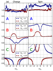
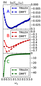
Figure 3: (color online) Left: Evolution of the local vertex $\mathrm{Re}\Lambda^{\eta}(i\omega_{n},i\Omega_{m})$ (half-filling, $t^{\prime}=0$). A, B and C are defined in Fig. 2. The dashed lines denote the atomic vertex $\Lambda_{\mathrm{at}}^{\eta}$ (Eq. (10)). Right: $\mathrm{Im}\Sigma_{\mathrm{loc}}(i\omega_{n})$ for TRILEX and DMFT (paramagnetic phase).

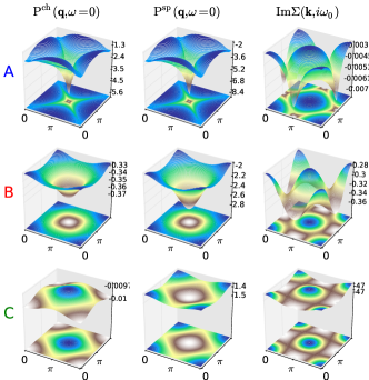
Figure 4: (color online) Momentum-dependence of the self-energy and polarization (half-filling, $t^{\prime}=0$). A, B and C are defined in Fig. 2. Left: $\mathrm{Re}P^{\mathrm{ch}}(\mathbf{q},\omega=0)$. Middle: $\mathrm{Re}P^{\mathrm{sp}}(\mathbf{q},\omega=0)$. Right: $\mathrm{Im}\Sigma(\mathbf{k},i\omega_{0})$.

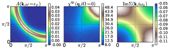
Figure 5: (color online) From left to right: $A(\mathbf{k},\omega=0)$, $\chi(\mathbf{q},i\Omega=0)$ and $\mathrm{Im}\Sigma(\mathbf{k},i\omega_{0})$ in the doped case: $U/D=1.8$, $t^{\prime}=-0.4t$, $\beta D=96$, $\delta=10\%$. ($xyz$-decoupling)

Let us now apply the TRILEX method to the Hubbard model on a square lattice. All energies are given in units of the half-bandwidth $D=4|t|$. The Brillouin zone is discretized on a $64\times 64$ momentum mesh. We restrict ourselves to the paramagnetic normal phase.

In Fig. 2, we present the phase diagram in the $(T,U)$ plane at half-filling. We obtain converged solutions of the TRILEX scheme above a temperature denoted $T_{\mathrm{AF}}^{xyz}$ (resp. $T_{\mathrm{AF}}^{z}$) for the $xyz$-decoupling (resp. $z$-decoupling). The evolution of the local vertex and self-energy (resp. lattice self-energy and polarizations) is presented in Fig.3 (resp. Fig. 4) for the points A, B and C of Fig. 2, in the $xyz$-decoupling. At weak coupling (point A), the local vertex $\Lambda$ reduces to the bare vertex $\lambda=1$ at large frequencies, up to numerical noise (Fig. 3a, upper panels). The spin polarization (hence the spin susceptibility, see Eq.(9)) becomes sharply peaked at the AF wavevector $\mathbf{Q}=(\pi,\pi)$ (Fig. 4, upper panels), reflecting the nesting features of the Fermi surface. As a result, the self-energy acquires a strong $\mathbf{k}$-dependence at $(\pi,0)$(Fig. 4), but its local part is the same as the DMFT self-energy (Fig.3b). At strong coupling (point C), the vertex becomes similar to the atomic vertex (Fig. 3a, lower panels). Furthermore, the self-energy and polarization are weakly momentum-dependent (Fig. 4, lower panels), in agreement with cluster DMFT calculations; the self-energy of TRILEX is very close to the DMFT self-energy (Fig. 3b). Finally, at intermediate coupling (point B), $\Lambda_{\mathrm{imp}}$ acquires frequency structures which interpolate between A and C (Fig. 3a, middle panels), while $\Sigma$ is strongly momentum-dependent and its local part departs from the DMFT self-energy (Fig. 3b, middle panels).

The temperature $T_{\mathrm{AF}}^{xyz/z}$ is determined by extrapolating the inverse static AF susceptibility (Fig.A.1 in Suppl. Mat.). It is reduced with respect to the Néel temperature computed in DMFT Kuneš (2011) as a result of nonlocal fluctuations beyond DMFT. Furthermore, $T_{\mathrm{AF}}^{xyz}\ll T_{\mathrm{AF}}^{z}$. As a consequence of the apparent divergence in the spin susceptibility at low temperatures (Fig. A.1), caused by a vanishing denominator of $W^{\eta}$ (Eq. 4b), we cannot obtain converged results in the close vicinity of and below $T_{\mathrm{AF}}$. Whether we have an actual AF transition or finite but very large correlation lengths (as seen e.g in Schäfer et al. (2015)), could be decided by generalizing the present formalism to the symmetry-broken phase. Contrary to cluster DMFT, the susceptibilities are not by-products of the calculation, but directly enter the self-consistency loop through $W^{\eta}$ (see Eq.(9)). We thus cannot converge paramagnetic solutions below an AF phase transition.

Let us now turn to the effect of doping. In Fig. 5, we present results for $t^{\prime}=-0.4t$, $\beta D=96$ and an intermediate interaction strength ($U=1.8$, close to point B). The spectral function displays Fermi arcs (Fig. 5, left panel), as observed in experiments Damascelli et al. (2003) and in cluster DMFT Jarrell et al. (2001); Kyung et al. (2004); Civelli et al. (2005); Kyung and Kotliar (2008); Kyung et al. (2006); Ferrero et al. (2008, 2009). Let us emphasize that this is obtained by solving a single-site quantum impurity problem, a far easier task than solving cluster impurities. The Fermi arc is a consequence of the large static spin susceptibility at the AF wavevector (Fig. 5, middle panel), which translates into a large imaginary part of the self-energy (Fig. 5, right panel). The corresponding variation of the spectral weight on the Fermi surface is rather mild due to the moderate correlation length ($\xi_{\mathrm{AF}}\sim 2$ unit spacings) for these parameters.

Alternative self-consistency conditions are possible, e.g $\chi_{\mathrm{loc}}^{\eta}=\chi_{\mathrm{imp}}^{\eta}$ instead of $W_{\mathrm{loc}}^{\eta}=W_{\mathrm{imp}}^{\eta}$ would enforce sum rules on two-particle quantities that are key to preserving the Mermin-Wagner theorem in Vilk et al. (1994); Katanin et al. (2009). However, this leads to a positive $\mathcal{U}^{\mathrm{sp}}(\tau)$ and hence to a severe sign problem in the quantum Monte-Carlo at low temperatures.

In conclusion, we have presented the TRILEX formalism, which encompasses long-range spin fluctuation effects and Mott physics in a unified way. Like DMFT, it can be systematically controlled by extending it to cluster schemes that interpolate between the single-site approximation studied in this paper, and the exact solution of the model. We expect that the convergence of the method as a function of the cluster size will strongly depend on the decoupling channel and, when done in the physically relevant channel, will be faster than cluster DMFT methods. Furthermore, because the competition between spin fluctuations and Mott physics can be described already at the single-site level, the method may be a good starting point for correlated multiorbital systems where spin fluctuations play an important role, like pnictides superconductors.

Supplementary Materials

Appendix A Atomic Vertex

In the atomic limit (single atomic site), one can compute the three-point vertex exactly by writing its Lehmann representation. One gets the following expression Ayral and Parcollet :

$$\Lambda_{\mathrm{at}}^{\eta=\mathrm{ch/sp}}(i\omega_{n},i\Omega_{m}) = \frac{1}{1-U^{\eta}\chi_{\mathrm{at}}^{\eta}\delta_{m}}\Bigg{(}\frac{U^{2}/4}{i\omega_{n}\left(i\omega_{n}+i\Omega_{m}\right)}+1$$ (10)

$$+\frac{U\beta\langle n_{\sigma}\rangle}{2}\left\{1-\frac{U^{2}}{4\left(i\omega_{n}\right)^{2}}\right\}\left\{\tanh\left(\frac{\beta U}{4}\right)\mp 1\right\}\delta_{m}\Bigg{)}$$

where $\chi_{\mathrm{\mathrm{at}}}^{\eta=\mathrm{ch/sp}}\equiv\frac{\beta}{2}\frac{e^{\mp\beta U/4}}{\cosh(\beta U/4)}$ and at half-filling, $\langle n_{\sigma}\rangle=1/2$.

Appendix B Computation of the three-leg vertex

$\Lambda_{imp}$ is computed from the fermionic three-point correlation function through the relation:

$$\Lambda_{\mathrm{imp}}^{\eta}(i\omega,i\Omega)=\frac{\tilde{\chi}_{\mathrm{imp,c}}^{\eta}(i\omega,i\Omega)}{G_{\mathrm{imp}}(i\omega)G_{\mathrm{imp}}(i\omega+i\Omega)\left(1-\mathcal{U}^{\eta}(i\Omega)\chi_{\mathrm{imp,c}}^{\eta}(i\Omega)\right)}$$ (11)

Here, the suffix “c” stands for “connected”, namely:

$$\tilde{\chi}_{\mathrm{imp,c}}^{\eta}(i\omega,i\Omega)\equiv\tilde{\chi}_{\mathrm{imp}}^{\eta}(i\omega,i\Omega)-\beta G_{\mathrm{imp}}(i\omega)\langle n_{\mathrm{imp}}^{\eta}\rangle\delta_{i\Omega}$$ (12)

while $\tilde{\chi}_{\mathrm{imp}}^{\eta}(i\omega,i\Omega)$ is defined as $\tilde{\chi}_{\mathrm{imp}}^{\mathrm{ch}/\mathrm{sp}}(i\omega,i\Omega)=\tilde{\chi}_{\mathrm{imp}}^{\uparrow\uparrow}(i\omega,i\Omega)\pm\tilde{\chi}_{\mathrm{imp}}^{\uparrow\downarrow}(i\omega,i\Omega)$, with:

$$\tilde{\chi}_{\mathrm{imp}}^{\sigma\sigma^{\prime}}(i\omega,i\Omega)\equiv\iint_{0}^{\beta}d\tau d\tau^{\prime}e^{i\omega\tau+i\Omega\tau^{\prime}}\langle Tc_{\sigma}(\tau)c_{\sigma}^{\dagger}(0)n_{\sigma^{\prime}}(\tau^{\prime})\rangle$$ (13)

$\chi_{\mathrm{imp}}^{\eta}(i\Omega)$ is the Fourier transform of $\chi_{\mathrm{imp}}^{\eta}(\tau)\equiv\langle Tn^{\eta}(\tau)n^{\eta}(0)\rangle_{\mathrm{c}}$.

Appendix C Inverse spin susceptibility: Temperature evolution

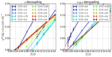
Figure A.1: (color online) Evolution of the inverse susceptibility with temperature (half-filling, $t^{\prime}=0$). The circles denote TRILEX computations, while the crosses on the $x$-axis are the extrapolated points. The dashed portion is the extrapolated line. Left: $z$-decoupling. Right: $xyz$-decoupling.

The inverse static AF spin susceptibility ($\chi^{\mathrm{sp}}(\mathbf{Q},i\Omega=0)^{-1}$, obtained from $W^{\mathrm{sp}}(\mathbf{q},i\Omega)$ by Eq. (9)) decreases linearly with temperature, as shown in Fig. A.1. This allows to determine $T_{\mathrm{AF}}$ by extrapolation. The resulting phase diagram is shown in Fig. 2.