ASPeRiX, a First Order Forward Chaining Approach for Answer Set Computing 111This work was supported by ANR (National Research Agency), project ASPIQ under the reference ANR-12-BS02-0003.
Abstract
The natural way to use Answer Set Programming (ASP) to represent knowledge in Artificial Intelligence or to solve a combinatorial problem is to elaborate a first order logic program with default negation. In a preliminary step this program with variables is translated in an equivalent propositional one by a first tool: the grounder. Then, the propositional program is given to a second tool: the solver. This last one computes (if they exist) one or many answer sets (stable models) of the program, each answer set encoding one solution of the initial problem. Until today, almost all ASP systems apply this two steps computation.
In this article, the project ASPeRiX is presented as a first order forward chaining approach for Answer Set Computing. This project was amongst the first to introduce an approach of answer set computing that escapes the preliminary phase of rule instantiation by integrating it in the search process. The methodology applies a forward chaining of first order rules that are grounded on the fly by means of previously produced atoms. Theoretical foundations of the approach are presented, the main algorithms of the ASP solver ASPeRiX are detailed and some experiments and comparisons with existing systems are provided.
KEYWORDS: Answer Set Programming, solver implementation, grounding on the fly, first order, forward chaining.
1 Introduction
Answer Set Programming (ASP) is a very convenient paradigm to represent knowledge in Artificial Intelligence (AI) and to encode combinatorial problems [Baral (2003), Niemelä (1999)]. It has its roots in nonmonotonic reasoning and logic programming and has led to a lot of works since the seminal paper [Gelfond and Lifschitz (1988)]. Beyond its ability to formalize various problems from AI or to encode combinatorial problems, ASP provides also an interesting way to practically solve such problems since some efficient solvers are available. In few words, if someone wants to use ASP to solve a problem, he has to write a logic program in term of rules in a purely declarative manner in such a way that the answer sets (initially called stable models in [Gelfond and Lifschitz (1988)]) of the program represent the solutions of his original problem.
Illustration of ASP formalism
Let us take two typical examples for which ASP is suitable: the first example is devoted to knowledge representation in Artificial Intelligence and the second one is a combinatorial problem.
KR problem
This first example deals with default reasoning on incomplete information. It consists in describing knowledge about birds.
The meaning of the two first rules is that we have two objects: titi which is a bird and lola which is an ostrich. The meaning of the other rules is that an ostrich is a bird, a bird which is not an ostrich flies and an ostrich does not fly. Here, we are interested in deducing some properties about titi and lola. Intuitively, we want that titi flies, lola is a bird and lola does not fly. Concerning the information that lola does not fly, let us notice that it is obtained by applying the last rule since lola is an ostrich and, then, the next to last rule cannot be applied in presence of ostrich lola due to the part not of this rule, called default negation. Here, there is only one answer set which contains all the deduced pieces of information: .
CSP problem
The second example deals with the representation of a combinatorial problem: possibles worlds are represented by nonmonotonic “guess” rules and choice between these worlds is expressed by constraints. The problem is then to find (at least) one solution corresponding to a world verifying the constraints. This example is about graph 2-coloring.
This represents a graph with two vertices and an edge between them (three first rules). The two following rules are guess rules. The fourth (resp. fifth) rule means that a vertex which is not colored in blue (resp. red) has to be colored in red (resp. blue). The two last rules are constraints. They mean that two adjacent vertices can not have the same color. Here, we want to find how the two vertices should be colored (knowing that two colors are available). Intuitively, we have two solutions: one with vertex 1 colored in blue and vertex 2 colored in red and the other one with vertex 1 colored in red and vertex 2 colored in blue. This corresponds to the two answer sets of the program: and . However, let us note that, in this kind of problem, we are often interested in finding one solution rather than finding all the possible solutions (and the determination of only one answer set is enough).
As regards the form of the rules, we can notice that a program usually contains different kind of rules. The simplest ones are facts as or representing data of the particular problem. Some ones are about background knowledge as . Some others can be nonmonotonic as for reasoning with incomplete knowledge. In other cases, especially for combinatorial problems, nonmonotonic rules can be used to encode alternative potential solutions of a problem as and expressing the two exclusive possibilities to color a vertex in a graph. Last, special headless rules are used to represent constraints of the problem to solve as , here, in order to not color with red two vertices linked by an edge.
With the examples above we can point out that knowledge representation in ASP is done by means of first order rules. But, from a theoretical point of view, answer set definition is given for propositional programs and the answer sets of a first order program are those of its ground instantiation with respect to its Herbrand universe (i.e. without variables). The first order program has to be seen as an intensional version of the grounded propositional corresponding program.
ASP systems
Concerning the ASP sytems, their main goal is how to compute answer sets in an efficient way. Let us recall some of their main features. Until today, almost all systems available to compute the answer sets of a program follow the architecture described in Fig. 1.
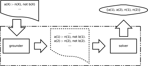
An ASP system begins its work by an instantiation phase in order to obtain a propositional program (and, as said above, the answer sets of the first order program will be those of its ground instantiation). After this first grounding phase realized by a grounder the solver starts the real phase of answer set computation by dealing with a finite, but sometimes huge, propositional program. The main goal of each grounding system is to generate all propositional rules that can be relevant for a solver and only these ones, while preserving answer sets of the original program. Current intelligent grounders simplify rules as much as possible. Simplifications can lead to compute the unique answer set of some programs (for instance, programs that does not contain default negation) but it is no longer possible once the problem is combinatorial. Anyway, the grounding phase is firstly and fully processed before calling the solver.
For the grounder box we can cite Lparse [Syrjänen (1998)] and Gringo [Gebser et al. (2011)], and for the solver box Smodels [Simons et al. (2002)] and Clasp [Gebser et al. (2012)]. A particular family of solvers are Assat [Lin and Zhao (2004)], Cmodels [Giunchiglia et al. (2006)] and Pbmodels [Liu and Truszczynski (2005)], since they transform the answer set computation problem into a (pseudo) boolean model computation problem and use a (pseudo) SAT solver as an internal black box. In the system DLV [Leone et al. (2006)], symbolized in Fig. 1 by the dash-line rectangle, the grounder ([Calimeri et al. (2008)] describes a parallel version) is incorporated as an internal function. In the same way, WASP [Alviano et al. (2013)] uses the DLV grounder [Faber et al. (2012)].
Grounding
The main drawback of the preliminary grounding phase is that it may lead to a lot of useless work as illustrated in the following examples.
The first examples illustrate the fact that the separation between the instantiation phase and the computation phase can prevent the (efficient) use of information relevant to the computation.
Example 1.
Let be the following ASP program:
Grounding of is infinite (if an upper bound for integers is not fixed) while it has a unique (and finite) answer set .
Let be the following ASP program:
From the program , current grounders generate roughly rules.
In both programs, because of the constraint that eliminates from the possible solutions every atom set containing , it is easy to see that rules for and for are useless since they can never contribute to generate an answer set of the corresponding program. In these useless rules are infinite while they are “only” large in : rules with positive body containing , like , and then, the rules with in their positive body are useless too. In defense of the actual grounders, their inability to eliminate these particular rules is not surprising since the reason justifying this elimination is the consequence of a reasoning taking into account the semantics of ASP. Thus, if we want to limit as much as possible the number of rules and atoms to deal with, we have not to separate grounding and answer set computing.
Example is a typical situation for planning problems where step must be generated only if the goal is not reached at step . Such situations are not tractable by grounders. That is the reason why the number of steps needed to reach the goal (or at least the maximum number of allowed steps) is given as input of planning problems (in ASP competition for example). Yet it is rather counterintuitive having to know the step number to solve the problem before solving.
The next example illustrates that the grounding phase generates too much information regarding the computation of one answer set.
Example 2.
Let be the program, as given in [Niemelä (1999)], encoding a 3-coloring problem on a vertices graph organized as a bicycle wheel (see below). stands for vertex, for edge, for color, for colored by, for not colored by.
![]() .
.
From , current grounders generate about rules. If is even then has no answer set and if is odd then it has 6 answer sets.
Suppose that has an answer set in which there is . Obviously, all the constraints like for all are necessary because they have to be checked. But, all the other constraints like , and for all can be considered as useless since vertex 1 is not colored by or . However, all these constraints have been generated. So, the time consumed by this task is clearly a lost time and the memory space used by these data could have been saved. Thus, if we are searching for a single answer set, a lot of work would be done for nothing since the grounded program contains the enumeration of all solutions when only one is searched.
The last exemple shows that when the number of solutions is very important ASP solvers have more difficulty to find one solution due to the grounding phase generating a lot of information concerning all the solutions.
Example 3.
Let be the program, inspired from one given in [Niemelä (1999)], encoding the Hamiltonian cycle problem in a vertices complete oriented graph. stands for vertex, for arc, for in Hamiltonian cycle, for not in Hamiltonian cycle, for start and for reached.
This program has answer sets. Whatever the number of desired solutions, current grounders generate about rules with predicate as head and about rules with predicate as head. Thus, even if we restrict our attention to the computation of one answer set, all the ASP solvers preceded by a grounding phase consume a huge amount of time when the graph has a few hundred vertices.
This previous example illustrates another strange phenomenon. Sometimes, solving a trivial problem, as finding one Hamiltonian cycle in a complete graph, is impossible for ASP systems. This is very counterintuitive since, in whole generality, in combinatorial problem solving the more solutions the problem has, the easier it is to find one of them. Again, the bottleneck for ASP systems seems to come from the huge number of rules and atoms that are generated in first, delaying and making the resolution more difficult than it should be.
Beyond these particular examples, the point to stress is that grounders generate in extension all the search space (for all potential solutions) that they give then to the solver. But, this is clearly not the approach of usual search algorithms. A classical coloring algorithm does not firstly enumerate, in extension, all possible colorations for every vertex in the graph. A finite domain solver makes choices by instantiating some variables, propagates the consequences of these choices, checks the constraints and by backtracking explores its search space. Following this strategy it instantiates and desinstantiates variables describing the problem to solve all along its search process. But, it does not build, a priori and explicitly, all the possible tuples of variables and constraints representing the problem to solve. That is why we think that if we want to use ASP to solve very large problems we have to realize the grounding process during the search process and not before it.
Is is important to notice that few works advocate the grounding of the program during the search of an answer set and not by a preprocessing. Some aim at solving the grounding bottleneck by combining ASP to constraint programming: [Baselice et al. (2005)] proposes to reduce the memory requirements for a very specific class of programs, i.e. multi-sorted logic programs with cardinality constraints, [Balduccini (2009)] proposes an algorithm to make cooperate an ASP solver and a Constraint Logic Programming solver in such a way that ASP is viewed as a specification language for constraint satisfaction problems and [Ostrowski and Schaub (2012)] describes the Clingcon system which is a tight cooperation between the ASP solver Clasp and the Constraint Programming solver GeCode. The theory solvers (mainly arithmetic solvers) forbid instances that are in conflict with the constraints reducing by this way the size of the grounding image. Some others works use a forward chaining of rules that are instantiated as and when required: GASP [Dal Palù et al. (2009)] and ASPeRiX [Lefèvre and Nicolas (2009a), Lefèvre and Nicolas (2009b)]) developed at the same time, and more recently OMiGA [Dao-Tran et al. (2012)]. They are all based on the notion of computation given in [Liu et al. (2010)]. GASP is implemented in Prolog and Constraint Logic Programming over finite domains. Each rule instantiation and propagation is realized by building and solving a CSP. OMiGA is implemented in Java and uses an underlying Rete network for instantiation and propagation. ASPeRiX, which is the one presented in this article, is implemented in C++. Instantiation and propagation are inspired by previous work realized on the DLV grounder which is based on the semi-naive evaluation technique of [Ullman (1989)].
Last, concerning a direct handling of first order programs, let us note that there exists some works [Gottlob et al. (1996), Eiter et al. (1997), Ferraris et al. (2007), Lin and Zhou (2007), Truszczynski (2012)] dealing with first order nonmonotonic logic programs. These works establish some relations between stable model semantics and constraints systems or second order logic or circumscription but they are not really concerned by the explicit computation of answer sets.
The present paper is an extended version of [Lefèvre and Nicolas (2009a), Lefèvre and Nicolas (2009b)]. It details our approach of answer set computation that escapes the preliminary grounding phase by integrating it in the search process and includes:
-
•
theoretical foundations of the approach, “mbt ASPeRiX computation”, with complete proofs; these computations are based on those of [Liu et al. (2010)] and include use of constraints and must-be-true propagation in order to guide the search;
-
•
a detailed description of the main algorithms;
-
•
experimentations of the resulting system, ASPeRiX, and comparisons with other similar systems and other “classical” ASP systems. Our methodology is particularly well suited for:
-
–
solving easy problems with a large grounding,
-
–
finding only one answer set for a program whose search space is large and proportional to the desired number of solutions,
-
–
solving problems for which pre-grounding is impossible because domains are infinite or open, or because some pieces of knowledge come from outside (distributed systems for example).
-
–
The paper is organized as follows. In Section 2 we recall the theoretical backgrounds about ASP necessary to the understanding of our work. In Section 3 we present our first order rule oriented approach of answer set computation and its implementation in the solver ASPeRiX. In Section 4 experimental results are presented. We conclude in Section 5 by citing some new perspectives for ASP as a result of our innovative approach. Proofs of theorems are reported in B.
2 Theoretical Background
In this section, we give the main backgrounds of ASP framework useful to the understanding of this article.
Set denotes the infinite countable set of variables, set denotes the set of function symbols, set denotes the set of constant symbols and set denotes the set of predicate symbols. It is assumed that the sets , , and are disjoint and that the set is not empty. Function denotes the arity function from to and from to which associates to each function or predicate symbol its arity. Set denotes the set of terms defined by induction as follows:
-
•
if then ,
-
•
if then ,
-
•
if with and then .
A ground term is a term built over only the two last items of the previous definition. The Herbrand universe is the set of all ground terms. Set denotes the set of atoms defined as follows:
-
•
if with then ,
-
•
if with and then .
A ground atom is an atom built over only ground terms. The Herbrand base denoted is the set of all ground atoms.
A normal logic program (or simply program) is a set of rules like
| (1) |
where are atoms.
The intuitive meaning of such a rule is: ”if all the ’s are true and it may be assumed that all the ’s are false then one can conclude that is true”. Symbol denotes the default negation. A rule with no default negation is a definite rule otherwise its is a nonmonotonic rule. A program with only definite rules is a definite logic program. A program is a propositional program if all the predicate symbols are of arity 0.
For each program , we consider that the set (resp. and ) consists of all constant (resp. function and predicate) symbols appearing in . These sets determine the set of ground terms and the set of ground atoms of the program. A substitution for a rule is a mapping from the set of variables from to the set of ground terms of . A ground rule is a ground instance of a rule if there is a substitution for such that , the rule obtained by substituting every variable in by the corresponding ground term in . The program (with variables) has to be seen as an intensional version of the program defined as follows: given a rule , is the set of all ground instances of and then, . Program may be considered as a propositional program. Let us note that the use of function symbols leads to an infinite Herbrand universe, this point will be discussed in Section 3.5.
Example 4.
The program
is a shorthand for the program
For a rule (or by extension for a rule set), we define:
-
•
its head,
-
•
its positive body and
-
•
its negative body.
The immediate consequence operator for a definite logic program is such that . The least Herbrand model of , denoted , is the smallest set of atoms closed under , i.e., the smallest set such that . It can be computed as the least fix-point of the consequence operator .
The reduct of a normal logic program w.r.t. an atom set is the definite logic program defined by:
and it is the core of the definition of an answer set.
Definition 1.
[Gelfond and Lifschitz (1988)] Let be a normal logic program and an atom set. is an answer set of if and only if .
For instance, the propositional program has two answer sets and .
Example 5.
Taking again the program , has four answer sets:
that are thus the answer sets of .
There is another definition of an anwer set for a normal logic program based on the notion of generating rules which are the rules participating to the construction of the answer set. These rules are important in our approach because they are exactly the rules fired in the ASPeRiX computation presented in the next section.
Definition 2.
[Konczak et al. (2006)] Let be a normal logic program and be an atom set. , the set of generating rules of , is defined as .
Definition 3.
[Konczak et al. (2006)] Let be a set of rules. is if there exists an enumeration of the rules of such that .
The next theorem is inspired by [Konczak et al. (2006)]. In [Konczak et al. (2006)], X is an answer set of a program if and only if . It can be reformulated by:
Theorem 1.
[Konczak et al. (2006)] Let be a normal logic program and be an atom set. Then, is an answer set of if and only if and is grounded.
Special headless rules, called constraints, are admitted and considered equivalent to rules like where is a new symbol appearing nowhere else. For instance, the program has one, and only one, answer set because constraint prevents to be in an answer set.
When dealing with default negation, we call a literal an atom, , or the negation of an atom, . A literal is said to be positive, and is said to be negative. The corresponding atom of a literal is denoted by . For a literal where , let us denote the function such that with the predicate symbol of the atom .
For purposes of knowledge representation, one may have to use conjointly strong negation (like ) and default negation (like ) inside a same program. This is possible in ASP by means of an extended logic program [Gelfond and Lifschitz (1991)] in which rules are built with classical literals (i.e. an atom or its strong negation ) instead of atoms only. Semantics of extended logic programs distinguishes inconsistent answer sets from absence of answer set. But, if we are not interested in inconsistent answer sets, the semantics associated to an extended logic program is reducible to answer set semantics for a normal logic program using constraints by taking into account the following conventions:
-
•
every classical literal is encoded by the atom ,
-
•
for every atom , the constraint is added.
By this way, only consistent answer sets are kept. In this article, we do not focus on strong negation and literal will never stand for classical literal.
Let us note that one can also use some particular atoms for (in)equalities and simple arithmetic calculus on (positive and negative) integers. Arithmetic operations are treated as a functional arithmetic and comparison relations are treated as built-in predicates.
Finally, a program is said to be stratified iff there is a mapping from to such that, for each ground rule like (1), the two following conditions hold:
-
•
for all
-
•
for all
3 A First Order Forward Chaining Approach for Answer Set Computing
3.1 ASPeRiX Computation
In this section, a characterization of answer sets for first-order normal logic programs, based on a concept of ASPeRiX computation, is presented. This concept is itself based on an abstract notion of computation for ground programs proposed in [Liu et al. (2010)]. This computation fundamentally uses a forward chaining of rules. It builds incrementally the answer set of the program and does not require the whole set of ground atoms from the beginning of the process. So, it is well suited to deal directly with first order rules by instantiating them during the computation.
The only syntactic restriction required by this methodology is that every rule of a program must be safe. That is, all variables occurring in the head and all variables occurring in the negative body of a rule occur also in its positive body. Note that this condition is already required by all standard evaluation procedures. Moreover, every constraint (i.e. headless rule) is considered given with the particular head and is also safe. For the moment we do not consider function symbols but their use will be discussed in Section 3.5.
An ASPeRiX computation is defined as a process on a computation state based on a partial interpretation which is defined as follows.
Definition 4.
A partial interpretation for a program is a pair of disjoint atom sets included in the Herbrand base of .
Intuitively, all atoms in belong to a search answer set and all atoms in do not.
The notion of partial interpretation defines different status for rules.
Definition 5.
Let be a ground rule and be a partial interpretation.
-
•
is supported w.r.t. when ,
-
•
is blocked w.r.t. when ,
-
•
is unblocked w.r.t. when ,
-
•
is applicable w.r.t. when is supported and not blocked.222The negation of blocked, not blocked, is different from unblocked.
An ASPeRiX computation is a forward chaining process that instantiates and fires one unique rule at each iteration according to two kinds of inference: a monotonic step of propagation and a nonmonotonic step of choice. To fire a rule means to add the head of the rule in the set .
Definition 6.
Let be a set of first order rules, be a partial interpretation and be a set of ground rules.
-
•
is the set of all supported definite rules and supported unblocked nonmonotonic rules from .
-
•
is the set of all applicable nonmonotonic rules from .
It is important to notice that the two sets defined above, like the set , do not need to be explicitly computed. It is in accordance with the principal aim of this work that is to avoid their extensive construction. When necessary, a first-order rule of can be selected and grounded with propositional atoms occurring in and in order to define a new (not already occurring in ) fully ground rule member of or . Because of the safety constraint on rules this full grounding is always possible. These mechanisms are specified in more details in Subsection 3.3. The sets and are used in the following definition of an ASPeRiX computation. Specific case of constraints (rules with as head) is treated by adding into set. By this way, if a constraint is fired (violated), should be added into and thus, would not be a partial interpretation.
Definition 7.
Let be a first order normal logic program. An ASPeRiX computation for is a sequence of ground rule sets and partial interpretations that satisfies the following conditions:
-
•
and ,
-
•
(Revision) ,
-
(Propagation) with
and -
or
(Rule choice) ,
with
and -
or
(Stability) and ,
-
-
•
(Convergence) .
The computation is said to converge to the set .
Example 6.
Let be the following program:
The following sequence is an ASPeRiX computation for :
The previous ASPeRiX computation converges to the set
which is an answer set for .
The following theorem establishes a connection between the results of any ASPeRiX computation and the answer sets of a normal logic program.
Theorem 2.
Let be a normal logic program and be an atom set. Then, is an answer set of if and only if there is an ASPeRiX computation , , for such that .
Let us note that in order to respect the revision principle of an ASPeRiX computation each sequence of partial interpretations must be generated by using the propagation inference based on rules from as long as possible before using the choice based on in order to fire a nonmonotonic rule. Then, because of the non determinism of the selection of rules from , the natural implementation of this approach leads to a usual search tree where, at each node, one has to decide whether or not to fire a rule chosen in . Persistence of applicability of the nonmonotonic rule chosen to be fired is ensured by adding to all ground atoms from its negative body. On the other branch, where the rule is not fired, the translation of its negative body into a new constraint ensures that it becomes impossible to find later an answer set in which this rule is not blocked.
Propagation can be improved by using “must-be-true”333The term “must be true” is first used in [Faber et al. (1999)]. atoms: atoms which have to be in the answer set to avoid a contradiction or, in other words, atoms already determined to be in but which are not yet be proved to be in.
Example 7.
Let be a constraint whose body contains only one literal with . In order to have an answer set, must be in so that the constraint is not applicable but is not yet proved (it is not the head of a fired rule). Thus, one can only conclude that must be true.
Must-be-true atoms can be used during the propagation step in order to reduce the search space.
Example 8.
Let be a rule with and but has been determined to be a must-be-true atom. The rule may be fired during the propagation step but one can only conclude that the rule head must be true (because is not yet proved).
Must-be-true atoms can also be used to reduce the size of , the set of nommonotonic rules that can be chosen to be fired.
Example 9.
Let be a rule with and but has been determined to be a must-be-true atom. The rule may already be considered to be blocked, even if is not yet proved, and thus may be excluded from .
Note that must-be-true atoms are first used to improve propagation and choice but have to be proved later, otherwise the computation can not lead to an answer set.
Notions of partial interpretation, rule status and ASPeRiX computation can be modified in order to consider these new elements.
Definition 8.
Let be a logic program. A mbt partial interpretation for is a triplet of disjoint atom sets included in the Herbrand base of .
Definition 9.
Let be a ground rule and be a mbt partial interpretation.
-
•
is supported w.r.t. when ,
-
•
is weakly supported w.r.t. when
-
•
is blocked w.r.t. when ,
-
•
is unblocked w.r.t. when ,
-
•
is applicable w.r.t. when is supported and not blocked.
Propagation is extended by Mbt-propagation: if some rule is weakly supported and unblocked w.r.t. mbt partial interpretation (but is not supported, i.e., does not belong to ), then the head of the rule can be added in set. And , the set of rules that can be chosen, is restricted to the rules that are not blocked w.r.t. mbt partial interpretation.
Definition 10.
Let be a set of first order rules, be a mbt partial interpretation and be a set of ground rules.
-
•
-
•
-
•
A mbt ASPeRiX computation is an ASPeRiX computation with this additional kind of propagation and with the possibility to block a rule from instead of firing it (“Rule exclusion”). To block a rule is to add a constraint with the negative literals of the rule body. If there is only one literal in the negative body, this constraint can be expressed by adding an atom in MBT set (see Example 7). These possibilities restrict rule choice in and thus forbid some computations: if a rule is blocked, computation can only converge to an answer set whose generating rules do not contain . Note that Convergence principle impose that, at the end of a computation, no constraint is applicable and each atom from MBT set has been proved (i.e., was moved from MBT to IN set).
Definition 11.
Let be a first order normal logic program. A mbt ASPeRiX computation for is a sequence of ground rule sets and and mbt partial interpretations that satisfies the following conditions:
-
•
, and ,
-
•
(Revision) ,
-
(Propagation) ,
with
and -
or
(Mbt-propagation) , ,
and
with -
or
(Rule choice) ,
,
,
with
and -
or
(Rule exclusion) ,
,-
,
and
with and -
or
, and
with and
-
-
or
(Stability) , and ,
-
-
•
(Convergence) .
Mbt ASPeRiX computations characterize answer sets of a normal logic program. Completeness and correctness are established by the following theorem.
Theorem 3.
Let be a normal logic program and be an atom set. Then, is an answer set of if and only if there is a mbt ASPeRiX computation , , for such that .
Note that computations model only successfull branches of a search tree. On the other hand, must-be-true atoms and rules blocking enable to prune failed branches of the tree and to reduce non determinism of the search by restricting the possible choices for the oracle (because some rules are explicitly excluded, and others are blocked by must-be-true atoms). So, these new elements do not improve the number of steps of a computation but they improve the number of steps needed to find a computation when there is no oracle to guide the search and, then, they make easier the search of answer sets.
3.2 ASPeRiX Main Algorithm
Now, we are interested in the practical computation of an answer set. The ASPeRiX algorithm, following the principle of mbt ASPeRiX computation seen in section 3.1, is based on the construction of three disjoint atom sets , and during the search for an answer set. It alternates two steps. On the one hand, a propagation step which instantiates all supported and unblocked rules which may be built from , and and fires them, i.e. adds their head in (or ). On the other hand, a choice step which forces or prohibits a nonmonotonic instantiated applicable rule to be fired during the next propagation step.
In order to treat the information more efficiently, the rules of a program are ordered following the strongly connected components () of the dependency graph of : the nodes of the dependency graph of a program are its predicate symbols and the arcs are defined by . The strongly connected components are ordered in such a way that if then no node (i.e. predicate symbol) of depends of a node of . A rule is said to belong to a SCC if the predicate symbol of its head is in the component . Note that constraints are not really concerned by ordering of rules but, for standardizing notations, constraints are considered to belong to a unique component whose number is greater than that of the last SCC, i.e., if is the last SCC then constraints are considered to belong to .
Example 10.
(Example 6 continued)
The strongly connected components (SCC) of the graph of the program are , and (Figure 2).
The ASPeRiX algorithm solves one by one the SCC of a program by starting by . When no propagation nor choice can no longer be done on the current SCC, the predicate symbols of the SCC are said to be solved and the SCC too. It means that nothing can be deduced anymore for those predicate symbols. The atoms which are instances of the predicate symbols of the current SCC and which are not in are implicitly added to . Note that they are not explicitly added to because ground instances of a predicate are not known (not computed): they could be infinite and, even if finite, to compute and store them is useless.
Rules of the program are instantiated on the fly during the propagation phase and the choice step. Hence the propositional program which contains all the instantiated rules of the program is never really computed. The propagation step and the choice step are realized in the ASPeRiX algorithm thanks to the functions and (which are selection functions in and sets used in the mbt ASPeRiX computation of Subsection 3.1). The function searches for a weakly supported unblocked rule amongst the current and next non-solved SCC. So propagation operates on several components: each rule is fired as soon as possible to quickly detect a possible conflict. Rules instantiated by are stored in a set during the answer set search to mark the substitution of rules that have already been used. For each first-order rule , denotes the set of all substitutions such that has already been fired. And is the set of instantiated rules obtained thanks to substitutions . The notation is extended to a set of first-order rules: . The function chooses an applicable rule in the current SCC when nothing can no longer be propagated. So choice, unlike propagation, operates only on the current component. This strategy, consisting of solving the SCC one after another, makes it possible to solve efficiently stratified programs (or some stratified parts of programs).
Functions and are specified in more details in Subsection 3.3 and are defined informally as follows:
-
•
: nondeterministic function which selects a rule (or a constraint) belonging to a SCC greater or equal to the current SCC in the dependency graph of a program such that , and or returns NULL if no such a rule exists.
-
•
: nondeterministic function which selects a rule belonging to the current SCC in the dependency graph of a program such that , and or returns NULL if no such a rule exists.
The function of Algorithm 1 specifies the algorithm of the search of one answer set for a program . The set is the set of constraints (rules with the symbol at their heads) of and the other rules. By default, is into the set . Then, if a constraint is fired, a contradiction is immediately detected since is added into the set and the sets and are no longer disjoint. The algorithm of the function computes one answer set (or none if the program is incoherent) thanks to the variable which stops the search once an answer set has been found. This algorithm may be easily extended to compute an arbitrary number of answer sets. Let us note that, for sake of simplicity, the function will return either a set (when there is an answer set) or the constant if there is no answer set.
The main parts of the function are now described. Initially, , , , is the index of the first SCC and .
The propagation phase successively fires each weakly supported and unblocked instantiated rule . At each step, the call selects and instantiates a unique unblocked rule such that (line 1). If such a rule exists, its head atom must belong to the answer set. This head atom is added into the set (line 1) if the positive body of the rule is included in the set or added into the set (line 1) otherwise since at least one atom of the positive body of the rule has not yet proved its membership to the set ( but ). Moreover, a head atom which is added into must be deleted from since a proof of its membership to the answer set has been found (line 1). When there is no more unblocked rule such that , is checked in order to detect a contradiction (line 1). If no contradiction is detected, the algorithm begins the choice step.
The choice point forces or forbids a nonmonotonic applicable rule to be fired. The call selects and instantiates a unique applicable rule of whose head belongs to the current SCC (line 1). If such a rule exists, is forced to be unblocked and then will be fired during the next propagation phase: its negative body is added to the set and function is recursively called with its new parameters (line 1). If a recursive call to the function detects a contradiction, the algorithm backtracks on the last choice point on the rule which has been forced to be fired and blocks it (lines 1-1): if is the only atom of the negative body of then is added to the set (line 1) else a constraint including all the atoms of the negative body of is added to the program (line 1). More precisely, the only atoms of the negative body that are considered are those with a predicate symbol belonging to the current SCC because atoms from a lower SCC are already solved, i.e. they are in or . When there is no more choice point, the current SCC is solved (line 1) but it must be checked that no atom of the set has a predicate symbol in the current SCC (line 1). If such an atom exists, and sets are not disjoint. Indeed, if a SCC is solved, atoms which are instances of predicate symbols of the SCC and which are not in are implicitly added to . Then if a atom is an instance of a predicate symbol of the current SCC, a failure is observed and the backtrack process continues (line 1). If the last SCC is solved, the set represents an answer set of if no constraint is applicable. This test is realized thanks to the nondeterministic function (line 1) which is specified in more details in Subsection 3.3 and is defined informally as follows:
: function which checks if there is any constraint such that , and .
Example 11.

The execution of the ASPeRiX algorithm for program of Example 6 is represented by a tree in Figure 3. At the beginning , , and the current SCC is the component . After the first propagation, and are in thanks to the two rules and . No choice point exists and the first SCC is solved since the set is empty. The component becomes the current SCC.
The first choice is realized on the current SCC (choice point ): the rule becomes unblocked by adding and into the set (left branch after choice point ). A new propagation phase shows that and are in since and can be fired. Then, a new choice is realized (choice point ) and the rule is forced to be unblocked (left branch after choice point ). The atom is added into the set . A new propagation phase shows that and are in since and can be fired. The second SCC is solved since no other rule is applicable and the set is still empty. In the same way, no propagation nor choice point is possible in the SCC . Since no constraint is applicable, a first answer set is obtained: .
If another answer set is wished, the algorithm backtracks to the last choice point on of the component and blocks the rule (right branch after choice point ) by adding a constraint into . A new choice is realized (choice point ) and the rule is forced to be unblocked (left branch after choice point ) by adding into the set. During the propagation step, is added into the set since is fired. The atom is then simultaneously in the sets and which leads to a contradiction.
The algorithm backtracks to the choice point of the component (choice point ) and the rule is blocked by adding the atom into the set (right branch after choice point ). Since there is no more possible choice and the set contains an atom whose predicate symbol is in the current SCC, this atom cannot be proved and this leads to a failure. The algorithm backtracks to the first choice point on of the component (choice point ) and blocks the rule and searches for a new possible answer set (right branch after choice point ). The process keeps going until the whole tree is computed when all the answer sets are required. Let us note that when dealing with the computation of one answer set like explained in the algorithm, only the first branch is considered.
3.3 Functions
Functions have a crucial role in two important steps of the search of an answer set. The function is called during the propagation step in order to choose the rules to fire and then to add their heads into (or ). The function is called during the choice step in order to force or to forbid a rule to be fired during the next propagation step. The function is called during the verification step in order to verify that no constraint is applicable. Since the principle of the solver ASPeRiX is to instantiate the rules on the fly during the search of an answer set, functions need to call a function which searches for a substitution for the atoms of a rule. This function is detailed in its own Subsection 3.4.
Function .
The function searches for a rule to fire w.r.t. , and sets. This function computes a complete instantiation of a rule such that the positive body is in and the negative body is in . The rule to instantiate is chosen amongst a set of rules consisting of rules that could lead to new, unprocessed instances. These rules are those whose body contains some predicate symbol of what we call an atom to propagate. Atoms to propagate are atoms recently added into , and sets, and not yet used for propagation phase. Thereby, when an atom is added into or (resp. ) set, the rules containing in their positive body (resp. negative body) will be in the set for the next call to in order to propagate this atom, i.e. to use its presence in or (resp. ) for building new instances of rules to be fired. During the first call of the function , atoms to propagate are the facts of the program, and the set contains all the rules which have some predicate symbols of the facts in their positive body. During a call after a choice point, atoms to propagate are those added into during this choice point, and the set contains all the rules which have some predicate symbols of these atoms in their negative body. During a call after the access to the next SCC, the predicate symbols of the current SCC are solved and then all instances of these predicate symbols that are not in are implicitly added into . Atoms to propagate are all these instances determined to be false, and then the set contains all the rules which have in their negative body some of these solved predicate symbols.
The Algorithm 2 of the function chooses a first-order rule amongst the set (the first one, line 2) and tries to find a weakly supported unblocked instantiation of the rule. It calls the function which returns this next instantiation if any (line 2). If there is no more weakly supported unblocked instantiated rule which may be extracted from (line 2), deletes from the rule and treats the next rule. This process is repeated until a weakly supported unblocked rule is found or there is no more rule in . When a rule allows a substitution (line 2), the latter is stored in in order to find some others at the next call to .
Example 12.
Example 11 is taken again. An answer set is searched after the choice point on the rule (choice point ): the atoms and are added into the set in order to force the rule to be fired (left branch after choice point ). During the propagation step, many calls to the function are executed. During the first call the set consists of all the rules containing in their negative body the predicate symbol of the atoms and that must be propagated. This set then contains the rules and Arbitrarily, the rule of the set is chosen and a supported unblocked instantiation is found. The function returns the instantiation of the rule and the function adds into . During the next call to , the set must contain, in addition to the previous rules, any rule containing in its positive body the predicate symbol of the atom to be propagated (since has been added into ). Since no rule respects this condition, the set still contains only the two previously added rules. The function searches for a new weakly supported unblocked instantiation of the rule . No such instantiation is found and the rule is deleted from the set . The function searches for a new weakly supported unblocked instantiation of the rule . The instantiation is then returned to the function which adds into . Then during the next call to the function , the set must be updated with the rules containing in their positive body the predicate symbol of the atom to propagate . As previously, no rule respects this condition and the set still contains the only rule . A new weakly supported unblocked instantiation is sought but this rule leads to a failure. The rule is then deleted from the set which becomes empty. Then the function returns the value NULL and the propagation step of the function stops.
Function .
The function is executed when no rule can be fired anymore and there is some SCC to be solved. This function searches an applicable instantiated rule belonging to the current SCC. The Algorithm 3 of function is similar to the algorithm of the function . The function searches for an applicable instantiated rule amongst a set of rules which have in their negative body at least one predicate symbol from the current SCC (otherwise, if all predicate symbols from negative body belong to previous SCC, they are already solved and then the rule can be considered as a monotonic one and is only used for propagation). The function chooses a rule in this set before calling the function searching for the next applicable instantiation for the considered rule. In a similar way as the function , the process is repeated until an applicable instantiated rule is found for a rule of or there is no more rule in .
Example 13.
Example 12 is taken again. After the first SCC has been solved, a first choice is realized on the current SCC, , by the function . The rules of this component which contains in their negative body at least one predicate symbol or of are added into the set of the rules that may be chosen. Then, the rules and are in . Arbitrarily, the function searches for an applicable instantiation of the first rule of this set and a choice point on is returned to the calling function (choice point ). After the propagation step, searches for a new applicable instantiation of the rule and a choice point on is returned to the calling function (choice point ). After a new propagation step, searches in vain a new applicable instantiation of the rule This last rule is then deleted from the set and searches for an applicable instantiation of the rule which leads to a failure. The set is now empty and the function returns NULL to the calling function to mean that no other choice may be realized on the current SCC.
Function .
The function is executed when no more choice point is possible for the last SCC. This function verifies that no constraint containing at least one predicate symbol of the last SCC is applicable in order to determine if the set is an answer set. The Algorithm 4 of the function is similar to the algorithm of the function . The function searches for an applicable instantiated constraint amongst a set of constraints whose negative body contains at least a not-solved predicate symbol of the last SCC. The function chooses a constraint in the set and calls the function which searches for an applicable instantiated constraint. If no instantiated constraint is applicable, the algorithm returns false and the set is an answer set of the program. If a constraint is applicable, the algorithm returns true which means there is a failure on the branch (the search of answer sets keeps going on other branches if any).
3.4 Rule Instantiation
In this section is described the process of instantiation of a rule. This process is a lazy one only called when needed. Since we only consider safe rules, the instantiation of a rule is in fact the instantiation of its positive body. In a forward chaining approach, the only rule instantiations of interest are those that lead to a not blocked supported rule or an unblocked weakly supported rule. Hence, the rule instantiation is mainly directed by the instantiated atoms already present in the sets and .
The algorithm used in the ASPeRiX solver and described below is inspired by the previous work realized on the DLV grounder [Faber et al. (2012), Perri et al. (2007)] which is based on the semi-naive evaluation technique of [Ullman (1989)]. The goal is to find a substitution for all the literals of the body of a rule thanks to the atoms already in , or . To do this, a partial substitution is built as possible values are found for the variables of the literals of the body of the rule . It is assumed that the literals , , …, of the body of the rule are ordered following a list : (resp. ) corresponds to (resp. ) and (resp. ) corresponds to the literal which precedes (resp. follows) the literal under consideration in the list. The substitution calculus for a literal of a rule is realized thanks to the functions and . These functions look for a substitution which has not already been computed, i.e. not leading to a substitution for present in the set of all substitutions such that has already been fired. If the literal is positive, a substitution such that the substituted atom is in the set (or ) is searched. If the literal is negative, (a) a substitution such that the substituted corresponding atom is in the set is searched if the goal is an unblocked rule or (b) the non membership of the substituted atom to the set is checked if the goal is a not blocked rule444In this case, the body of the rule is ordered in such a way that negative literals appear after the positive literals containing their variables..
In the functions and which follow, the parameter shows if an unblocked weakly supported or not blocked supported rule is looked for.
-
•
is a function which searches for the first possible substitution for a literal w.r.t. the sets , and , selection criterion (unblocked weakly supported or applicable rule) and the current partial substitution . returns true and updates the partial substitution in case of success. Otherwise, the function returns false.
-
•
is a function which searches for the next possible substitution for literal given the already realized substitutions.
For a rule , a free variable of a literal is an occurrence of a variable such that it is its first occurrence in the body of when starting traversing the literal . In other words, no other literal which precedes in the body of contains an occurrence of the variable . During the instantiation of a rule, a possible substitution is sought for all the free variables of every traversed literal and the substitutions of the previously calculated variables are kept. If a literal has no free variable, the validity of the substitution w.r.t. the selection criterion is checked (i.e. the substituted corresponding atom is in or if and is in or is not in if ).
Example 14.
Let be a rule. The ordered list of the body of the rule is with:
-
•
-
•
-
•
.
Function of Algorithm 5 specifies the instantiation principles of a rule for constant sets , and . This function is initialized with the partial substitution which is the last found substitution (thanks to the function ) for the rule if any (line 5). If it is the first attempt for the instantiation of this rule, is empty (line 5) and the function searches a first substitution for the first literal of the body of the rule using the function . Otherwise, a substitution for has already been computed (line 5), the function searches a new possible substitution for the rule. For this, the function searches the next possible instance of the last literal of the rule by deleting from the substitutions of the free variables of this literal (thanks to the function ) and by calling the function . During the execution of the main loop, the function first checks if a substitution has been found for the current literal (line 5). If it is the case, it searches a first substitution for the next literal of the rule body respecting the partial substitution . When all the atoms have been considered, a complete substitution is found (line 5). The function returns this substitution. When the instantiation of a literal fails (i.e. there is no possible substitution for it), the function backtracks on the previous literal (line 5) and updates by deleting the substitutions of the free variables of this literal. Hence the function calls the function which searches the next possible instantiation for this literal. The instantiation of a rule fails when no more substitution is possible for the first literal (line 5).
Actually, the instantiation algorithm of a rule is slightly more complicated than the Algorithm 5 since the atoms dynamically added into , and sets during the answer set computation, called atoms to propagate, have to be taken into account: if possible, each substitution has to be computed once and only once. Hence ASPeRiX uses a queue called (resp. and ) which contains the atoms to be added into the set (resp. and ). When all the instances of a rule , for given sets , and , have been generated, an atom to propagate whose predicate symbol appears in the body of the rule is extracted. Now denotes the mbt partial interpretation obtained by adding into . The body of the rule is ordered in such a way that the first literals are those whose predicate symbol is the one of the atom to propagate (they are the literals that might unify with ). Then these literals whose predicate symbol is are successively marked and placed at the beginning of the rule. The marked literal might only take the value of the atom to propagate whereas the following (non marked) literals might take any values in . Then, if the instantiation of the first literal fails, it is unmarked, the next literal of predicate becomes the first literal of the rule body and is marked in turn, and the instantiation of the rule is started again. The unmarked literals might then take any values in (which excludes the values of already used) while the marked literal can only take the value of the atom to propagate, and the non marked literals always take their values in . If the instantiation of the first literal fails and there is no other literal to be marked, the instantiation of the rule fails.
Example 15.
Let be a rule and , and be sets of atoms defined as follow:
| *** first call to *** | |||||
| (1.1) | - | - | ( marked) | ||
| (1.2) | - | ||||
| (1.3) | complete instantiation | ||||
| *** second call to *** | |||||
| (2.1) | NO | ||||
| (2.2) | NO | - | |||
| (2.3) | NO | - | - | failure | |
| (2.4) | - | - | ( marked) | ||
| (2.5) | NO | - | failure | ||
The atom has to be propagated by instantiating the rule . Table 1 shows the different steps of the instantiation. The literals to be marked (whose predicate symbol is ) of the body of the rule are and . These literals are placed at the beginning of the body of like this: . In Table 1, for clarity, the sequence of literals of the rule body is not changed when the marked literal changes. But the marked literal (shown in bold) is processed first, which is the same. The first attempt for an instantiation begins and for the first time with atom to propagate . The literal is then marked and takes as unique value that of the atom to propagate ((1.1) Table 1). Hence, value is substituted to the variable in . Then, the following literal in the body of the rule, , becomes the current literal and takes as value the first amongst those into which is also . Hence, value is substituted to the variable in ((1.2) Table 1). Then the last literal, , is reached. This literal has no free variable and the membership into is simply checked for which is obtained from by substituting and by the values in ((1.3) Table 1). There is no more literal to consider then a complete substitution has been found. The atom of the head takes the values of the substitution . Hence, the forward chaining algorithm can add into the queue.
Now, during a new instantiation attempt of the rule for the atom to propagate , the function restarts with the last substitution of the rule in order to find a new substitution for the literal . The second attempt for an instantiation begins with atom to propagate for the second time. Since has no free variable, there can be no other substitution than the current one ((2.1) Table 1). The process then backtracks to the literal which has no other substitution in ( has been inferred after and is not into the current set ) ((2.2) Table 1). Since literal can only take the value , it also fails ((2.3) Table 1). Since the last literal has failed, the literal is now marked instead of , and is instantiated with the atom to propagate . Hence, value is substituted to the variable in ((2.4) Table 1). Literal is unmarked and can only take the values of the atoms of , thus no substitution is possible. Hence the algorithm fails on the first literal ((2.5) Table 1). Since there is no more literal to be marked, the rule instantiation ends by a failure for the atom to propagate . The sets becomes as follow:
| *** third call to *** | |||||
| (1.1) | - | - | ( marked) | ||
| (1.2) | - | ||||
| (1.3) | NO | ||||
| (1.4) | - | ||||
| (1.5) | NO | ||||
| (1.6) | NO | - | |||
| (1.7) | NO | - | - | failure | |
| (1.8) | - | - | ( marked) | ||
| (1.9) | - | ||||
| (1.10) | complete instantiation | ||||
| *** fourth call to *** | |||||
| (2.1) | NO | ||||
| (2.2) | NO | - | |||
| (2.3) | - | NO | - | failure | |
The next atom is extracted from the queue to propagate. The third attempt for an instantiation of begins with atom to propagate for the first time. Table 2 shows the different steps of the instantiation. The literals and are again to be marked. The rule instantiation is restarted with the literal which is the marked literal. The variable is substituted by the value since the only allowed value is that of the atom to propagate ((1.1) Table 2). The current literal is now where is substituted by the value since is into ((1.2) Table 2). The literal has no free variable and since the atom which respects the substitution is not in , the literal has no possible substitution ((1.3) Table 2). Then a new instantiation for is sought: its next possible value is (since is in ) ((1.4) Table 2). Again, since the atom which respects the substitution is not in , the literal has no possible substitution ((1.5) Table 2). The process backtracks to the literal which has no possible value ((1.6) Table 2). Hence, the process backtracks to the literal which has no possible value since the only possible value was that of the atom to propagate ((1.7) Table 2). Since the first literal has failed, the process restarts by marking the second literal (and unmarking the first ). The marked literal is processed first, it substitutes by the value of the atom to propagate ((1.8) Table 2). The unmarked literal may only take its values into . The variable is then substituted by the value ((1.9) Table 2). The literal has no free variable and since which respects the substitution is in a complete substitution is found ((1.10) Table 2). The atom of the head takes then the value of the substitution . Hence, the forward chaining algorithm can add into and into .
Then, during a new instantiation attempt of the rule , the atom to propagate is still . The process restarts from the last substitution and search for a new substitution for the literal . A fourth attempt for an instantiation begins with atom to propagate for the second time. Since has no free variable, there can be no other substitution than the current one ((2.1) Table 2). The process then backtracks to the literal that has no other substitution since the only possible values are those from (then neither the atom to propagate nor appeared after are possible) ((2.2) Table 2). The literal also fails since the marked literal only accepts the value of the atom to propagate ((2.3) Table 2). Since there is no more literal to be marked, the instantiation of the failing rule ends for this atom to propagate. The process continues with the atom which also leads to a failure.
3.5 ASPeRiX language
The core language of ASPeRiX is that of normal logic programs [Gelfond and Lifschitz (1988)] with function symbols and true (or strong) negation without inconsistent answer set. ASPeRiX also provides dedicated treatment of lists with built-in predicates, as in DLV-complex [Calimeri et al. (2008)], an extension of DLV with lists and sets. On the other side, ASPeRiX does not provide aggregate atoms and optimization statements [Buccafurri et al. (2000)] which are accepted by the main current systems.
One of the important issues in ASP is the treatment of function symbols. Uninterpreted function symbols are important because they enable representation of recursive structures such as lists and trees. But reasoning becomes undecidable if no restriction is enforced. A lot of work has been made for identifying program classes for which reasoning is decidable [Alviano et al. (2011), Alviano et al. (2010), Calimeri et al. (2011), Lierler and Lifschitz (2009), Baselice and Bonatti (2010), Greco et al. (2013)].
The inherent difficulty with functions in general (and arithmetic in particular) in the framework of ASP is that it makes the Herbrand universe infinite in whole generality. ASP grounders Lparse [Syrjänen (1998)] and versions up to 3.0 of Gringo [Gebser et al. (2007)] accept programs respecting some syntactic domain restrictions and are able to deal with some restricted versions of functions.
DLV grounder [Faber et al. (2012)] and Gringo (since version 3.0) [Gebser et al. (2011)] only require programs to be safe and can deal with all programs having a finite instantiation. DLV guarantees finite instantiation for finitely ground programs but membership in this class is not decidable. It integrates a Finite Checker module which can check if a program belongs to a sub-class of finitely ground programs (argument-restricted programs). For programs that are not member of this sub-class, answer sets can be computed without preliminary check but ending is not guaranteed.
ASPeRiX can deal with these programs and with some other programs whose instantiation is infinite but whose answer sets are finite. For example, the program from Section 1 is not finitely ground: intelligent instantiation of the program must be finite to be finitely ground. The key points of intelligent instantiation are that rules are instantiated with atoms appearing in head of rules of the program, and simplifications are performed relatively to facts and rule heads of preceding components of the dependency graph. In example , choice between and makes both possible for the grounder, and constraint has no effect on intelligent instantiation of the program. Thus, the grounding of rules from will be the same with or without the constraint : infinite in both cases. ASPeRiX halts on and is thus able to halt on non finitely ground programs but it is not able to verify in advance if answer sets are finite or not, and thus if computation will end or not. Nevertheless, ending can be guaranteed by means of command-line options specifying the maximum allowed nesting level for functional terms and the biggest admissible integer (DLV grounder provides similar possibilities). These restrictions ensure that our computations always converge to an answer set if it exists. Formalizing the class of programs for which ASPeRiX halts will be the subject of a forthcoming work.
4 Experimental results
Following Algorithm 1 of Section 3.2, the solver called ASPeRiX has been implemented in C++ and is available at http://www.info.univ-angers.fr/pub/claire/asperix.
There are two other ASP systems, GASP [Dal Palù et al. (2009)] and OMiGA [Dao-Tran et al. (2012)], that realize the grounding of the program during the search of an answer set.
GASP is an implementation in Prolog and Constraint Logic Programming over finite domains of the notion of computation (see Section 3.1). The main ideas are the same as those of ASPeRiX. Notable differences are the following. Well founded consequences of the program are computed first. Then propagation is close to ours. GASP does not deal with must-be-true atoms but two special cases of propagation, not treated by ASPeRiX, are implemented: (a) if the head of a rule is known to be in OUT set and the body of the rule is satisfied except for one positive literal, then this literal must be false (added to OUT) and (b) if, for some undefined atom , there is no applicable rule whose head is , then can be added to OUT. For each rule, instantiation and propagation are realized by building and solving a CSP that determines atoms derivable from the rule. Representation of interpretations uses Finite Domain Sets, such a data structure is efficient to represent compactly intervals but it need to code tuples (instances of predicates) by integers (very big integers if domain is large and arity of predicate too). This representation impose the set of ground terms of the program to be finite and thus function symbols are excluded. On the other hand, GASP supports some cardinality constraints. To our knowledge, GASP remained at the prototype stage and is no longer developed.
OMiGA is implemented in Java. Functional symbols (of non-zero arity) are not supported. Principles of propagation and choice are the same as those of ASPeRiX but implementation uses Rete algorithm for improving the speed of propagation. First order rules are represented by a Rete network. Each node represents a literal (or a set of literals) from the body of a rule or the atom of the head of a rule. It stores all instances of the node that are true w.r.t. current partial interpretation. Thereby all partial instantiations of rules are stored in the network. This lead to an efficient propagation regarding computation time, but memory space is sacrified. Dependency graph and solved predicates seems to be treated in a similar manner to that of ASPeRiX. Current version [Weinzierl (2013)] uses must-be-true propagation and tries to introduce methods for conflict-driven learning of non-ground rules: when a constraint is violated, a new constraint is built by unfolding of rules whose firing contributes to the conflict. This learned constraint is then transformed into special rules so as to be used for propagation.
In the following we give some results of evaluation of ASPeRiX 0.2.5 highlighting its adequacy to some particular problems. It is compared with Clingo (composed by Gringo 3.0.5 and Clasp 1.3.10) [Gebser et al. (2011), Gebser et al. (2012)], DLV Dec 16 2012 [Leone et al. (2006)], GASP (june 2009) [Dal Palù et al. (2009)] and OMiGA Dec 3 2012 [Dao-Tran et al. (2012)]. Version without learning is used for OMiGA because learning lowers its performances. All the systems have been run on an Intel Core i7-3520M PC with 4 cores at 2.90GHz and about 4GB RAM, running Linux Ubuntu 12.04 64 bits. For each instance of a problem, the memory usage is limited to 3.000MB and computation time to 600 seconds. RunLim1.7 is used for these limitations tasks. Tables of results use (resp. ) to indicate Out of Memory (resp. Out of Time). Results for GASP are only given for the first two examples, because it does not accept other tested programs.
Schur problem
The Schur number problem is to partition numbers into sets such that all of the sets satisfy: if and are assigned to the same set, then is not in the set. The following program [Dal Palù et al. (2009)] is for sets and numbers.
The results are shown in Table 3 for . reports the number of answer sets which are all computed. For all , Schur- has no answer set.
The program is a typical “guess and check” program. The seach space is expressed by the three rules with as head predicate, and constraint eliminates “bad choices”. The grounding of the program is rather small but the search space is large. The problem is very easy for Clingo and DLV but very hard for ASPeRiX and GASP. Systems using grounding on the fly have to repeat instantiation of the same rules in each branch of the search tree. Moreover, constraints are not efficiently managed by systems like ASPeRiX: it does not use constraints for propagation but only checks if a constraint is violated. Compared to ASPeRiX, OMiGA performs well for computation time, certainly because Rete network improve speed of instantiation (partial instantiations are stored in the network) and the network remains relatively small in such an example. This example illustrates a large class of programs that ASPeRiX mismanage: programs with many choices and little propagation by forward chaining.
| ASPeRiX | Clingo | DLV | OMiGA | GASP | |||
| time in sec | 0.1 | 0.1 | 0.1 | 0.1 | 0.1 | ||
| memory in MB | 2.0 | 2.0 | 2.0 | 20.0 | 4.4 | ||
| time in sec | 0.1 | 0.1 | 0.1 | 0.1 | 0.1 | ||
| memory in MB | 2.0 | 2.0 | 2.0 | 20.0 | 5.2 | ||
| time in sec | 0.1 | 0.1 | 0.1 | 0.1 | 0.3 | ||
| memory in MB | 2.0 | 2.0 | 2.0 | 20.0 | 6.3 | ||
| time in sec | 0.1 | 0.1 | 0.1 | 0.2 | 1.0 | ||
| memory in MB | 2.0 | 2.0 | 2.0 | 24.0 | 8.3 | ||
| time in sec | 0.1 | 0.1 | 0.1 | 0.3 | 3.6 | ||
| memory in MB | 2.0 | 2.0 | 2.0 | 50.0 | 8.3 | ||
| time in sec | 0.1 | 0.1 | 0.1 | 0.4 | 11.0 | ||
| memory in MB | 2.0 | 2.0 | 2.0 | 63.0 | 8.3 | ||
| time in sec | 0.3 | 0.1 | 0.1 | 0.6 | 41.0 | ||
| memory in MB | 2.0 | 2.0 | 2.0 | 99.0 | 7.5 | ||
| time in sec | 1.0 | 0.1 | 0.1 | 0.8 | 113.0 | ||
| memory in MB | 2.0 | 2.0 | 2.0 | 100.0 | 5.7 | ||
| time in sec | 3.6 | 0.1 | 0.1 | 1.3 | 370.0 | ||
| memory in MB | 2.0 | 2.0 | 2.0 | 165.0 | 7.5 | ||
| time in sec | 11.1 | 0.1 | 0.1 | 1.9 | OoT | ||
| memory in MB | 2.0 | 2.0 | 2.0 | 220.0 | - | ||
| time in sec | 39.7 | 0.1 | 0.1 | 2.8 | OoT | ||
| memory in MB | 2.2 | 2.0 | 2.0 | 290.0 | - | ||
| time in sec | 131.0 | 0.1 | 0.1 | 4.1 | OoT | ||
| memory in MB | 2.2 | 2.0 | 2.0 | 290.0 | - | ||
| time in sec | 448.0 | 0.1 | 0.1 | 6.5 | OoT | ||
| memory in MB | 2.2 | 2.0 | 2.0 | 285.0 | - | ||
| time in sec | OoT | 0.1 | 0.1 | 11.0 | OoT | ||
| memory in MB | - | 2.0 | 2.0 | 287.0 | - | ||
Conversely, the following examples illustrate problems for which grounding on the fly is well adapted.
Birds problem
Problem birds is a stratified program encoding a taxonomy about flying and non flying birds. stands for , for , for , for , for , and for .
We add to this program the atoms encoding birds with of ostriches, of penguins whose half of them are super penguins.


The unique answer set of such a program can be computed polynomially. ASPeRiX uses only propagation step, without choice point, and grounders completely evaluate the program so that the solver has nothing to do. Experimental results for birds are comparable for ASPeRiX, Clingo, GASP and DLV. ASPeRiX has the best results for CPU time, and DLV for memory usage (Figure 4 and 5). For such a problem, the number of instantiated rules must be nearly the same for all systems. On the other side, OMiGA system uses a very large amount of memory space, certainly due to the Rete network which is designed to sacrifice memory for increased speed. Unfortunately, memory gains expected by the first order approach are lost.
Cutedge problem
cutedge program is proposed in [Dao-Tran et al. (2012)]: given a random graph with 100 vertices and edges, each answer set is obtained by deleting an edge and compute some transitive closure on the remaining edges.
| ASPeRiX | Clingo | DLV | OMiGA | |||
| time in sec | 0.1 | 21 | 115 | 0.6 | ||
| memory in MB | 14.8 | 345 | 103 | 85 | ||
| time in sec | 0.2 | 21 | 226 | 1.8 | ||
| memory in MB | 14.8 | 345 | 103 | 200 | ||
| time in sec | 2.7 | 32 | OoT | 11.4 | ||
| memory in MB | 15.1 | 345 | - | 1042 | ||
| time in sec | 16 | 78 | OoT | 48 | ||
| memory in MB | 16.4 | 345 | - | 1050 | ||
| time in sec | 36 | 123 | OoT | 84 | ||
| memory in MB | 18.0 | 345 | - | 1050 | ||
| time in sec | 167 | 189 | OoT | 165 | ||
| memory in MB | 24.1 | 345 | - | 1050 | ||
| time in sec | 0.1 | 60 | 325 | 1 | ||
| memory in MB | 23.7 | 881 | 144 | 177 | ||
| time in sec | 0.5 | 63 | OoT | 3.7 | ||
| memory in MB | 23.8 | 881 | - | 425 | ||
| time in sec | 5.8 | 94 | OoT | 29 | ||
| memory in MB | 24.0 | 881 | - | 1100 | ||
| time in sec | 30.7 | 228 | OoT | 125 | ||
| memory in MB | 25.3 | 881 | - | 1150 | ||
| time in sec | 67 | 373 | OoT | 245 | ||
| memory in MB | 27 | 881 | - | 1190 | ||
| time in sec | 0.1 | 94 | 465 | 1 | ||
| memory in MB | 28.5 | 1167 | 202 | 132 | ||
| time in sec | 0.8 | 94 | OoT | 5 | ||
| memory in MB | 28.6 | 1168 | - | 680 | ||
| time in sec | 7.6 | 114 | OoT | 41 | ||
| memory in MB | 29.1 | 1168 | - | 1135 | ||
| time in sec | 42 | 210 | OoT | 192 | ||
| memory in MB | 31.3 | 1168 | - | 1125 | ||
| time in sec | 92 | 316 | OoT | 352 | ||
| memory in MB | 34.1 | 1168 | - | 1132 | ||
Computing each answer set is only based on propagation, and the number of answer sets equals the number of edges. The number of rules needed to compute all answer sets is proportional to while the rule number needed to compute one is proportional to . But systems with pregrounding phase must generate all ground instances of rules even if only one answer set is required. The results are shown in Table 4. ASPeRiX has the best results for this program both for CPU time and memory usage. OMiGA and Clingo use much more memory and are much slower than ASPeRiX. As expected, memory usage of Clingo is independent of the number of answer sets required and is close to the square of that used by ASPeRiX. For its part, DLV quickly exceeds the time limit imposed.
Hamiltonian cycle problem
The program (see Example 3), Hamiltonian cycle in a complete graph, is another easy problem with a lot of answer sets. Each answer set is easy to compute but the whole instantiation is huge. Experiments for the computation of one answer set in a graph with vertices are represented in Figures 6 and 7. ASPeRiX performs well on this example whereas OMiGA has time and memory problems similar to that of Clingo and DLV. One more time, a simple problem becomes intractable by systems with pregrounding phase because they drown it in a lot of useless information so that memory used quickly becomes prohibitive.


Hanoi problem
Hanoi example illustrates a planning problem where the maximum number of allowed steps is given as input. is the number of disks in the problem and is the maximum number of moves that are allowed to move all disks from the first rod to the third. The least value of is the minimum required to achieve the goal, then its value is gradually increased to evaluate its impact. The complete program is given in A and experimental results are shown in Table 5. ASPeRiX performances are (almost) independent of the given number of moves: search, and therefore grounding, are stopped when a solution is found. Conversely, grounders are quickly overwhelmed as they are obliged to fully instantiate the program with all hypothetical (and unnecessary in this case) calculation steps555 iClingo [Gebser et al. (2008)] was created to address this specific problem. Some directives are added to the program in order to incrementally instantiate some predicates of the program. But it does not escape the grounding/solving separation, it only introduces some tools to control the process. . This example cannot be computed by OMiGA due to restrictions on the input language it accepts (function symbols are not supported).
| ASPeRiX | Clingo | DLV | |||
| time in sec | 0.1 | 0.1 | 0.1 | ||
| memory in MB | - | - | - | ||
| time in sec | 0.1 | 0.7 | 0.8 | ||
| memory in MB | - | 27 | 22 | ||
| time in sec | 0.1 | 1.5 | 3.6 | ||
| memory in MB | - | 54 | 51 | ||
| time in sec | 0.1 | 11.6 | - | ||
| memory in MB | - | 327 | OoM | ||
| time in sec | 0.1 | 27 | - | ||
| memory in MB | - | 693 | OoM | ||
| time in sec | 0.1 | 66 | - | ||
| memory in MB | - | 1523 | OoM | ||
| time in sec | 0.1 | - | - | ||
| memory in MB | - | OoM | OoM | ||
| time in sec | 0.1 | - | - | ||
| memory in MB | - | OoM | OoM | ||
| time in sec | 0.1 | - | - | ||
| memory in MB | 12.9 | OoM | OoM | ||
| time in sec | 0.3 | - | - | ||
| memory in MB | 23.9 | OoM | OoM | ||
| time in sec | 0.2 | 0.1 | 0.1 | ||
| memory in MB | 3.7 | 6.4 | 4 | ||
| time in sec | 0.2 | 0.7 | 0.9 | ||
| memory in MB | 3.7 | 28 | 31 | ||
| time in sec | 0.2 | 8.2 | 9.4 | ||
| memory in MB | 3.8 | 245 | 270 | ||
| time in sec | 0.2 | 91 | - | ||
| memory in MB | 3.8 | 2055 | OoM | ||
| time in sec | 0.2 | - | - | ||
| memory in MB | 3.8 | OoM | OoM | ||
| time in sec | 0.2 | - | - | ||
| memory in MB | 4.8 | OoM | OoM | ||
| time in sec | 0.2 | - | - | ||
| memory in MB | 5.8 | OoM | OoM | ||
| time in sec | 0.4 | - | - | ||
| memory in MB | 14.4 | OoM | OoM | ||
| time in sec | 0.7 | - | - | ||
| memory in MB | 25 | OoM | OoM | ||
| time in sec | 4.7 | 0.6 | 1.1 | ||
| memory in MB | 10.3 | 24 | 29 | ||
| time in sec | 4.7 | 9 | - | ||
| memory in MB | 10.3 | 272 | OoM | ||
| time in sec | 4.7 | 83 | - | ||
| memory in MB | 10.3 | 1863 | OoM | ||
| time in sec | 4.7 | - | - | ||
| memory in MB | 10.3 | OoM | OoM | ||
| time in sec | 4.7 | - | - | ||
| memory in MB | 10.4 | OoM | OoM | ||
| time in sec | 4.7 | - | - | ||
| memory in MB | 10.5 | OoM | OoM | ||
| time in sec | 4.7 | - | - | ||
| memory in MB | 11.3 | OoM | OoM | ||
| time in sec | 4.8 | - | - | ||
| memory in MB | 12.4 | OoM | OoM | ||
| time in sec | 5 | - | - | ||
| memory in MB | 21 | OoM | OoM | ||
| time in sec | 5.6 | - | - | ||
| memory in MB | 31.7 | OoM | OoM | ||
Three coloring problem
The program (see Example 2), 3-coloring problem on a graph organized as a bicycle wheel, poses no problem for Clingo and DLV (cf. Table 6). But ASPeRiX and OMiGA have bad results on this example because they are mismanaging constraints. Once a vertex is colored, say , constraint prohibits coloring adjacent vertices of the same color. In propositional systems, unit propagation (or equivalent) works well and allows to infer that adjacent vertices are not colored red. But first-order approach does not allow, in general case, to use unit propagation and thus, constraints are mainly used for verification and not for propagation. A lot of work remains on these points. First-order constraints could instead allow more powerful propagation. Suppose for example a constraint and is added in set then, for all , can be excluded at once from current solution, even if values are potentially infinite. But these opportunities are not exploited yet.
| ASPeRiX | Clingo | DLV | OMiGA | |||
| time in sec | 0.1 | 0.1 | 0.1 | 0.3 | ||
| memory in MB | 2 | 1 | 1 | 45 | ||
| time in sec | 3.4 | 0.1 | 0.1 | 7.7 | ||
| memory in MB | 1.8 | 1 | 1 | 132 | ||
| time in sec | 0.1 | 0.1 | 0.1 | OoT | ||
| memory in MB | 3 | 1.5 | 1.1 | - | ||
| time in sec | OoT | 0.1 | 0.1 | OoT | ||
| memory in MB | - | 1.8 | 1.4 | - | ||
| time in sec | 1.6 | 0.1 | 0.1 | OoT | ||
| memory in MB | 8.8 | 3.3 | 3.3 | - | ||
| time in sec | OoT | 0.1 | 0.3 | OoT | ||
| memory in MB | - | 3.3 | 3.3 | - | ||
| time in sec | 13.3 | 0.1 | 0.1 | OoT | ||
| memory in MB | 15.9 | 5.5 | 5.5 | - | ||
| time in sec | OoT | 0.1 | 1.4 | OoT | ||
| memory in MB | - | 5.5 | 5.5 | - | ||
To sum up, ASPeRiX is efficient to deal with stratified programs or simple problems whose instantiation is infinite or huge but much of which is useless to compute one specific answer set. On the other hand, the system is not competitive for more combinatorial problems, with a large search space and few solutions, because propositional methods for propagation, heuristics, learning lemmas did not apply to the first order case.
5 Conclusion
In this paper, we have presented the ASPeRiX approach to answer set computation. Our methodology deals with first order rules following a forward chaining with grounding process realized on the fly and has been implemented in the ASP solver ASPeRiX. This paper is the first comprehensive document in which a survey of the important techniques relevant to our approach is presented.
Starting from a short description of state-of-the-art ASP working principle, we have presented by many examples the main motivation of our approach: escaping the bottleneck of the preliminary phase of grounding in which many state-of-the-art systems fall. After a presentation of the theoretical foundations of ASP, we have described by an ASPeRiX computation our first order forward chaining approach for answer set computing and have established the soundness and completeness of this calculus w.r.t. the semantics of ASP (Proofs are reported in B). We have then described in details the main algorithms of ASPeRiX and particularly those which realize the selection of the first order rules to be instantiated and applied according to the current answer set in construction.
Our methodology allows very good performances for definite and stratified programs. It outperforms systems with a pregrounding phase for programs with large grounding but much of it is unnecessary to solve the problem. On the other side, performances quickly degrade for combinatorial problems with large search spaces, especially if forward chaining propagation can not be exploited.
We have shown that our approach escapes the bottleneck of the preliminary phase of grounding that is the only difficulty for some classes of programs. A direct consequence of our new approach is that the use of symbolic functions in general and arithmetic calculus in particular inside ASP is greatly facilitated.
The forward chaining with the grounding process realized on the fly as an operational semantics emphasizes the programming aspect of ASP in which the answer set is not only the result of a black box but the result of a process that may be followed. This is interesting when dealing with knowledge coming from the web and expressed in description logic since the structure of information uses rules that are chained ones with the others (whereas this is not always the case for a program encoding a combinatorial problem). Moreover, when dealing with knowledge expressed in description logic, one important issue is the ability to query the knowledge base. The grounding process realized on the fly will then allow to focus only on the rules useful to find an answer to the query. For this category of programs, we think that our approach may be of great interest.
Furthermore, computing the answer sets of a program is a fundamental goal but not an exclusive one. Debugging a program, controlling its behavior, introducing in it some features coming from other programming languages may be of great interest for ASP. We think that our methodology of answer set computing, guided by the rules of the program, is the good starting point towards these new goals.
The ASPeRiX project is still in progress. Improvements at the algorithmic level are underway by the development and implementation of backjumping and clause learning techniques. On the other hand, we plan to fully respect the core language ASP [Calimeri et al. (2014)] by introducing, among others, minimization / maximization and aggregates and extend it by introducing existentially quantified variables in multi-head rules to encode fragments of Description Logics which are logical formalisms for ontologies and the Semantic Web.
Tribute
In memory of the late Pascal Nicolas who was at the origin of this work. He sadly passed away in 2010 but his enthusiasm, his passion for research and his great humanity are still with us.
References
- Alviano et al. (2011) Alviano, M., Calimeri, F., Faber, W., Ianni, G., and Leone, N. 2011. Function Symbols in ASP: Overview and Perspectives. In Nonmonotonic Reasoning, Essays Celebrating its 30th Anniversary, G. Brewka, V. Marek, and M. Truszczynski, Eds. Studies in Logic, vol. 31. College Publications, 1–24.
- Alviano et al. (2013) Alviano, M., Dodaro, C., Faber, W., Leone, N., and Ricca, F. 2013. WASP: A native ASP solver based on constraint learning. In Proceedings of the 12th International Conference on Logic Programming and Nonmonotonic Reasoning (LPNMR’13), P. Cabalar and T. C. Son, Eds. LNCS, vol. 8148. Springer, 55–67.
- Alviano et al. (2010) Alviano, M., Faber, W., and Leone, N. 2010. Disjuntive ASP with functions: Decidable queries and effective computation. Theory and Practice of Logic Programming 10, 4-6, 497–512.
- Balduccini (2009) Balduccini, M. 2009. Representing constraint satisfaction problems in answer set programming. In Proceedings of the Workshop on Answer Set Programming and Other Computing Paradigms (ASPOCP’09). 16–30.
- Baral (2003) Baral, C. 2003. Knowledge Representation, Reasoning and Declarative Problem Solving. Cambridge University Press.
- Baselice et al. (2005) Baselice, S., Bonatti, P., and Gelfond, M. 2005. Towards an integration of answer set and constraint solving. In Proceedings of the 21st International Conference on Logic Programming (ICLP’05). LNCS, vol. 3668. Springer, 52–66.
- Baselice and Bonatti (2010) Baselice, S. and Bonatti, P. A. 2010. A decidable subclass of finitary programs. Theory and Practice of Logic Programming 10, 4-6, 481–496.
- Buccafurri et al. (2000) Buccafurri, F., Leone, N., and Rullo, P. 2000. Enhancing disjunctive datalog by constraints. IEEE Transactions on Knowledge and Data Engineering 12, 5, 845–860.
- Calimeri et al. (2008) Calimeri, F., Cozza, S., Ianni, G., and Leone, N. 2008. Computable functions in ASP: Theory and implementation. In Proceedings of the 24th International Conference on Logic Programming (ICLP’08), M. G. de la Banda and E. Pontelli, Eds. LNCS, vol. 5366. Springer, 407–424.
- Calimeri et al. (2011) Calimeri, F., Cozza, S., Ianni, G., and Leone, N. 2011. Finitely recursive programs: Decidability and bottom-up computation. AI Communications 24, 4 (Dec.), 311–334.
- Calimeri et al. (2014) Calimeri, F., Ianni, G., and Ricca, F. 2014. The third open answer set programming competition. Theory and Practice of Logic Programming 14, 1, 117–135.
- Calimeri et al. (2008) Calimeri, F., Perri, S., and Ricca, F. 2008. Experimenting with parallelism for the instantiation of ASP programs. Journal of Algorithms 63, 1-3, 34–54.
- Dal Palù et al. (2009) Dal Palù, A., Dovier, A., Pontelli, E., and Rossi, G. 2009. Gasp: Answer set programming with lazy grounding. Fundamenta Informaticae 96, 3 (Aug.), 297–322.
- Dao-Tran et al. (2012) Dao-Tran, M., Eiter, T., Fink, M., Weidinger, G., and Weinzierl, A. 2012. OMiGA: An open minded grounding on-the-fly answer set solver. In Proceedings of the 13th European Conference on Logics in Artificial Intelligence (JELIA’12). LNAI, vol. 7519. Springer, 480–483.
- Eiter et al. (1997) Eiter, T., Lu, J. J., and Subrahmanian, V. S. 1997. Computing non-ground representations of stable models. In Proceedings of the 4th International Conference on Logic Programming and Nonmonotonic Reasoning (LPNMR’97), J. Dix, U. Furbach, and A. Nerode, Eds. LNCS, vol. 1265. Springer, 198–217.
- Faber et al. (2012) Faber, W., Leone, N., and Perri, S. 2012. The intelligent grounder of DLV. In Correct Reasoning - Essays on Logic-Based AI in Honour of Vladimir Lifschitz, E. Erdem, J. Lee, Y. Lierler, and D. Pearce, Eds. LNCS, vol. 7265. Springer, 247–264.
- Faber et al. (1999) Faber, W., Leone, N., and Pfeifer, G. 1999. Pushing goal derivation in dlp computations. In Proceedings of the 5th International Conference on Logic Programming and Nonmonotonic Reasoning (LPNMR’99), M. Gelfond, N. Leone, and G. Pfeifer, Eds. LNCS, vol. 1730. Springer, 177–191.
- Ferraris et al. (2007) Ferraris, P., Lee, J., and Lifschitz, V. 2007. A new perspective on stable models. In Proceedings of the 20th International Joint Conference on Artificial Intelligence (IJCAI’07). 372–379.
- Gebser et al. (2008) Gebser, M., Kaminski, R., Kaufmann, B., Ostrowski, M., Schaub, T., and Thiele, S. 2008. Engineering an incremental ASP solver. In Proceedings of the 24th International Conference on Logic Programming (ICLP’08), M. Garcia de la Banda and E. Pontelli, Eds. LNCS, vol. 5366. Springer, 190–205.
- Gebser et al. (2011) Gebser, M., Kaminski, R., König, A., and Schaub, T. 2011. Advances in gringo Series 3. In Proceedings of 11th International Conference on Logic Programming and Nonmonotonic Reasoning (LPNMR’11), J. P. Delgrande and W. Faber, Eds. LNCS, vol. 6645. Springer, 345–351.
- Gebser et al. (2012) Gebser, M., Kaufmann, B., and Schaub, T. 2012. Conflict-driven answer set solving: From theory to practice. Artificial Intelligence 187, 52–89.
- Gebser et al. (2007) Gebser, M., Schaub, T., and Thiele, S. 2007. GrinGo : A New Grounder for Answer Set Programming. In Proceedings of the 9th International Conference on Logic Programming and Nonmonotonic Reasoning (LPNMR’07). LNCS, vol. 4483. Springer, 266–271.
- Gelfond and Lifschitz (1988) Gelfond, M. and Lifschitz, V. 1988. The stable model semantics for logic programming. In Proceedings of the Fifth International Conference and Symposium on Logic Programming (ICLP’88), R. A. Kowalski and K. Bowen, Eds. The MIT Press, Cambridge, Massachusetts, 1070–1080.
- Gelfond and Lifschitz (1991) Gelfond, M. and Lifschitz, V. 1991. Classical negation in logic programs and disjunctive databases. New Generation Computing 9, 3/4, 365–386.
- Giunchiglia et al. (2006) Giunchiglia, E., Lierler, Y., and Maratea, M. 2006. Answer set programming based on propositional satisfiability. Journal of Automated Reasoning 36, 4, 345–377.
- Gottlob et al. (1996) Gottlob, G., Marcus, S., Nerode, A., Salzer, G., and Subrahmanian, V. S. 1996. A non-ground realization of the stable and well-founded semantics. Theoretical Computer Science 166, 1-2, 221–262.
- Greco et al. (2013) Greco, S., Molinaro, C., and Trubitsyna, I. 2013. Logic programming with function symbols: Checking termination of bottom-up evaluation through program adornments. Theory and Practice of Logic Programming 13, 4-5, 737–752.
- Konczak et al. (2006) Konczak, K., Linke, T., and Schaub, T. 2006. Graphs and colorings for answer set programming. Theory and Practice of Logic Programming 6, 61–106.
- Lefèvre and Nicolas (2009a) Lefèvre, C. and Nicolas, P. 2009a. A first order forward chaining approach for answer set computing. In Proceedings of the 12th International Conference on Logic Programming and Nonmonotonic Reasoning (LPNMR’09). LNCS, vol. 5753. Springer, 196–208.
- Lefèvre and Nicolas (2009b) Lefèvre, C. and Nicolas, P. 2009b. The first version of a new ASP solver : ASPeRiX. In Proceedings of the 12th International Conference on Logic Programming and Nonmonotonic Reasoning (LPNMR’09). LNCS, vol. 5753. Springer, 522–527.
- Leone et al. (2006) Leone, N., Pfeifer, G., Faber, W., Eiter, T., Gottlob, G., Perri, S., and Scarcello, F. 2006. The DLV system for knowledge representation and reasoning. ACM Transactions on Computational Logic 7, 3, 499–562.
- Lierler and Lifschitz (2009) Lierler, Y. and Lifschitz, V. 2009. One more decidable class of finitely ground programs. In Proceedings of the 25th International Conference on Logic Programming (ICLP’09). LNCS, vol. 5649. Springer, 489–493.
- Lin and Zhao (2004) Lin, F. and Zhao, Y. 2004. ASSAT: computing answer sets of a logic program by SAT solvers. Artificial Intelligence 157, 1-2, 115–137.
- Lin and Zhou (2007) Lin, F. and Zhou, Y. 2007. From answer set logic programming to circumscription via logic of GK. In Proceedings of the 20th International Joint Conference on Artificial Intelligence (IJCAI’07). 441–446.
- Liu et al. (2010) Liu, L., Pontelli, E., Son, T. C., and Truszczynski, M. 2010. Logic programs with abstract constraint atoms: The role of computations. Artificial Intelligence 174, 3-4, 295–315.
- Liu and Truszczynski (2005) Liu, L. and Truszczynski, M. 2005. Pbmodels - software to compute stable models by pseudoboolean solvers. In Proceedings of the 8th International Conference on Logic Programming and Nonmonotonic Reasoning (LPNMR’05), C. Baral, G. Greco, N. Leone, and G. Terracina, Eds. LNCS, vol. 3662. Springer, 410–415.
- Niemelä (1999) Niemelä, I. 1999. Logic programs with stable model semantics as a constraint programming paradigm. Annals of Mathematics and Artificial Intelligence 25, 3-4, 241–273.
- Ostrowski and Schaub (2012) Ostrowski, M. and Schaub, T. 2012. ASP modulo CSP: the clingcon system. Theory and Practice of Logic Programming 12, 4-5, 485–503.
- Perri et al. (2007) Perri, S., Scarcello, F., Catalano, G., and Leone, N. 2007. Enhancing DLV instantiator by backjumping techniques. Annals of Mathematics and Artificial Intelligence 51, 2-4, 195–228.
- Simons et al. (2002) Simons, P., Niemelä, I., and Soininen, T. 2002. Extending and implementing the stable model semantics. Artificial Intelligence 138, 1-2, 181–234.
- Syrjänen (1998) Syrjänen, T. 1998. Implementation of local grounding for logic programs for stable model semantics. Tech. rep., Helsinki University of Technology.
- Truszczynski (2012) Truszczynski, M. 2012. Connecting first-order ASP and the logic FO(ID) through reducts. In Correct Reasoning - Essays on Logic-Based AI in Honour of Vladimir Lifschitz. LNCS, vol. 7265. Springer, 543–559.
- Ullman (1989) Ullman, J. D. 1989. Principles of Database and Knowledge-Base Systems, Volume II. Computer Science Press.
- Weinzierl (2013) Weinzierl, A. 2013. Learning non-ground rules for answer-set solving. In 2nd Workshop on Grounding and Transformations for Theories With Variables (GTTV’13).
Appendix A Hanoi example
The following ASP program is the example with 4 discs.
%------ Initial settings
number_of_moves(10000).
largest_disc(4).
%------ Initial state
initial_state(towers(l(4,l(3,l(2,l(1,nil)))),nil,nil)).
% ------ Goal state
goal(towers(nil, nil, l(4,l(3,l(2,l(1,nil)))))).
% ------ all discs involved ------
disc(1..4).
% ------ legal stacks ------
legalStack(nil).
legalStack(l(T,nil)) :- disc(T).
legalStack(l(T,l(T1,S))) :- legalStack(l(T1,S)), disc(T), T > T1.
% ------ possible moves ------
possible_state(0,towers(S1,S2,S3))
:- initial_state(towers(S1,S2,S3)),
legalStack(S1), legalStack(S2), legalStack(S3).
possible_state(I,towers(S1,S2,S3))
:- possible_move(I,T,towers(S1,S2,S3)).
% From stack one to stack two.
possible_move(J,towers(l(X,S1),S2,S3),towers(S1,l(X,S2),S3))
:- possible_state(I,towers(l(X,S1),S2,S3)),
number_of_moves(N), I<=N, legalStack(l(X,S2)), J=I+1, not ok(I).
% From stack one to stack three.
possible_move(J,towers(l(X,S1),S2,S3),towers(S1,S2,l(X,S3)))
:- possible_state(I,towers(l(X,S1),S2,S3)),
number_of_moves(N), I<=N, legalStack(l(X,S3)), J=I+1, not ok(I).
% From stack two to stack one.
possible_move(J,towers(S1,l(X,S2),S3),towers(l(X,S1),S2,S3))
:- possible_state(I,towers(S1,l(X,S2),S3)),
number_of_moves(N), I<=N, legalStack(l(X,S1)), J=I+1, not ok(I).
% From stack two to stack three.
possible_move(J,towers(S1,l(X,S2),S3),towers(S1,S2,l(X,S3)))
:- possible_state(I,towers(S1,l(X,S2),S3)),
number_of_moves(N), I<=N, legalStack(l(X,S3)), J=I+1, not ok(I).
% From stack three to stack one.
possible_move(J,towers(S1,S2,l(X,S3)),towers(l(X,S1),S2,S3))
:- possible_state(I,towers(S1,S2,l(X,S3))),
number_of_moves(N), I<=N, legalStack(l(X,S1)), J=I+1, not ok(I).
% From stack three to stack two.
possible_move(J,towers(S1,S2,l(X,S3)),towers(S1,l(X,S2),S3))
:- possible_state(I,towers(S1,S2,l(X,S3))),
number_of_moves(N), I<=N, legalStack(l(X,S2)), J=I+1, not ok(I).
%------ actual moves ------
% a solution exists if and only if there is a "possible_move"
% leading to the goal.
% in this case, starting from the goal, we proceed backward
% to the initial state to single out the full set of moves.
% Choose from the possible moves.
move(I,towers(S1,S2,S3))
:- goal(towers(S1,S2,S3)), possible_state(I,towers(S1,S2,S3)).
ok(I) :- move(I,towers(S1,S2,S3)), goal(towers(S1,S2,S3)).
win :- ok(I).
:- not win.
move(J,towers(S1,S2,S3))
:- move(I,towers(A1,A2,A3)),
possible_move(I,towers(S1,S2,S3),towers(A1,A2,A3)), J=I-1,
not nomove(J,towers(S1,S2,S3)).
nomove(J,towers(S1,S2,S3))
:- move(I,towers(A1,A2,A3)),
possible_move(I,towers(S1,S2,S3),towers(A1,A2,A3)), J=I-1,
not move(J,towers(S1,S2,S3)).
%------ precisely one move at each step ------
moveStepI(I) :- move(I,T).
:- legalMoveNumber(I), ok(J), I<J, not moveStepI(I).
:- legalMoveNumber(I), move(I,T1), move(I,T2), T1!=T2.
legalMoveNumber(0).
legalMoveNumber(K)
:- legalMoveNumber(I), number_of_moves(J), I < J, K=I+1.
#hide.
#show move/2.
Appendix B Proofs
B.1 Proof of Theorem 1
Proof.
(of Theorem 1) Let be a normal logic program and . Let us note first that if is grounded then .
If is an answer set of then, by a theorem from (Konczak et al. 2006), is grounded and, also according to (Konczak et al. 2006), . Since , we can conclude .
Let us now suppose that and is grounded. We have , then and, according to (Konczak et al. 2006), is an answer set of .
∎
B.2 Proof of Theorem 2
We first give some material needed in the proof. Auxiliary Lemma 1 is used in the proof of Lemma 2. Lemmas 2 and 3 establish completeness and correctness.
Lemma 1 shows that the generating rules of a program can be ordered so as to correspond to the order of application of rules in an ASPeRiX computation. Condition (1) says that a rule used at step is supported at this step. Condition (2) says that if a rule is a member of at step but is used at a later stage , then all rules used at steps between and are members of at step . In other words, condition (2) says that propagation is entirely completed before making a choice.
Lemma 1.
Let be a normal logic program and be an answer set of . Then, there exists an enumeration of , the set of generating rules of , such that for all the following two conditions are satisfied:
-
(1)
-
(2)
for all , if and then .
Proof.
(of Lemma 1) Let be a normal logic program and be an answer set of . By Theorem 1, there exists an enumeration of such that , , i.e. such that condition (1) is satisfied. This enumeration can be recursively modified in the following way in order to verify condition (2). For each , if satisfies (2) then remains at rank , else there exists with that falsifies condition (2). In this last case, it suffices to swap the two rules in the enumeration to satisfy condition (2) at rank . ∎
Notation. If is a normal logic program and is a sequence of ground rule sets and partial interpretations , then denotes and denotes .
Lemma 2.
Let be a normal logic program and be an answer set of . Then there exists an ASPeRiX computation that converges to .
Proof.
(of Lemma 2) Let be a normal logic program and be an answer set of . Then, there exists an enumeration of that satisfies conditions (1) and (2) from Lemma 1.
Let be the sequence defined as follows.
-
•
, and
-
•
, , and
-
•
, , and
For all , we have:
-
(enumi1)
(by Theorem 1)
-
(enumi2)
and (by (*1))
-
(enumi3)
and therefore (by Definition 2 of )
-
(enumi4)
Property (*4) can be proved as follows. By definition 6, . And by (*2) and (*3), and . Thus .
We are now able to prove that the sequence is an ASPeRiX computation.
Let us first note that is a partial interpretation since (by (*2) and (*3)).
Now we prove that Revision principle holds for each . Let such that , then is such that . Two cases are possible. First, if , then and Revision principle holds at rank . Second, if then, by definition of enumeration , there is no rule with such that and . So . And as (by (*4)), . Moreover, is a generating rule, thus and (since ). Thereby and Revision principle holds. If , Revision principle trivially holds (Stability).
At step , we have and . . Thus . Convergence principle holds and . ∎
Lemma 3.
Let be a normal logic program and be an ASPeRiX computation for . Then, is an answer set of .
Proof.
(of Lemma 3) Let be an ASPeRiX computation for .
We first prove that . For each rule , and set increases monotonically, thus . If , then and . Since and sets grow monotonically with an empty intersection, . If , then . And, since , we have , and thus, with the same reasonning as above (), .
and, since , . Thus .
By Convergence principle we have , then . Since , . And (by definition of an ASPeRiX computation), thus .
Moreover, for all , , thus is grounded and, since , is grounded. Finally, by Theorem 1, is an answer set of P.
∎
B.3 Proof of Theorem 3
Lemma 4.
Let be a normal logic program and be an answer set for . Then there exists a mbt ASPeRiX computation for that converges to X.
Proof.
Lemma 5.
Let be a normal logic program and be a mbt ASPeRiX computation for . Then is an answer set of .