Application of the Hamiltonian formulation to nonlinear light-envelope propagations

Abstract

A new approach, which is based on the new canonical equations of Hamilton found by us recently, is presented to analytically obtain the approximate solution of the nonlocal nonlinear Schrödinger equation (NNLSE). The approximate analytical soliton solution of the NNLSE can be obtained, and the stability of the soliton can be analytically analysed in the simple way as well, all of which are consistent with the results published earlier. For the single light-envelope propagated in nonlocal nonlinear media modeled by the NNLSE, the Hamiltonian of the system can be constructed, which is the sum of the generalized kinetic energy and the generalized potential. The extreme point of the generalized potential corresponds to the soliton solution of the NNLSE. The soliton is stable when the generalized potential has the minimum, and unstable otherwise. In addition, the rigorous proof of the equivalency between the NNLSE and the Euler-Lagrange equation is given on the premise of the response function with even symmetry.

.

I Introduction

The propagations of the (1+D)-dimensional light-envelopes in nonlinear media have been studied extensively for a few decades Agrawal-book-01 ; Assanto-book-2012 ; Trillo-book-ss ; Kivshar-book-os ; Stegeman-science-1999 ; Chen-rpp-2012 ; Malomed-job-2005 , which are governed by the following dimensionless model Guo-book-2015 :

$$i\frac{\partial\varphi}{\partial z}+\nabla_{\bot}^{2}\varphi+\Delta n\varphi=0,$$ (1)

where $\varphi(\mathbf{r},z)$ is the complex amplitude envelop, $\Delta n(\mathbf{r},z)$ is the light-induced nonlinear refractive index, $z$ is the longitudinal coordinate, $\mathbf{r}$ is the $D$-dimensional transverse coordinate vector with $D$ being the positive integer, and $\nabla_{\bot}$ is the $D$-dimensional differential operator vector of the transverse coordinates. Generally, $\Delta n(\mathbf{r},z)$ can be phenomenologically expressed as the convolution between the response function $R(\mathbf{r})$ of the media and the modulus square of the light-envelope $\varphi(\mathbf{r},z)$ for the bulk media with the nonlocal nonlinearity Guo-book-2015 ; Guo-book-2012 ; Snyder-science-97 ; Krolikowski-pre-01

$$\Delta n(\mathbf{r},z)=\int_{-\infty}^{\infty}R(\mathbf{r}-\mathbf{r}^{\prime})|\varphi(\mathbf{r}^{\prime},z)|^{2}\mathrm{d}^{D}\mathbf{r}^{\prime}.$$ (2)

According to the relative scale of the characteristic length of the response function R and the scale in the transverse dimension occupied by the light-envelope $\varphi$, the degree of nonlocality can be divided into four categoriesGuo-book-2015 ; Krolikowski-pre-01 ; Guo-book-2012 : local, weakly nonlocal, generally nonlocal, and strongly nonlocal, and locality is the case when the response function R is the Dirac delta function. In the local case, Eq.(1) is reduced to

$$i\frac{\partial\varphi}{\partial z}+\nabla_{\bot}^{2}\varphi+|\varphi|^{2}\varphi=0.$$ (3)

Eq. (1) together with the nonlocal nonlinearity (2) is called as the nonlocal nonlinear Schrödinger equation (NNLSE) Guo-book-2015 ; Guo-book-2012 ; Krolikowski-pre-01 , while its special case, Eq. (3), is the well-known nonlinear Schrödinger equation (NLSE) Kivshar-book-os ; Agrawal-book-01 ; Trillo-book-ss .

The NNLSE (with its special case NLSE) can describe the nonlinear propagations of the optical beams Assanto-book-2012 ; Trillo-book-ss ; Stegeman-science-1999 ; Chen-rpp-2012 ; Kivshar-book-os , the optical pulses Agrawal-book-01 ; Kivshar-book-os and the optical pulsed beams Kivshar-book-os ; Malomed-job-2005 . The second term of the NNLSE accounts for the diffraction for the first case where $\mathbf{r}$ is the spatial transverse coordinate, the group velocity dispersion (GVD) for the second case where $\mathbf{r}$ is the time coordinate, and both the diffraction and the GVD for the last case where $\mathbf{r}$ is both the spatial transverse coordinate and the time coordinate, while the third term (the nonlinear term) describes the compression of the light-envelopes for all cases. Specifically, when $D=1$, the NNLSE can model the propagation of the optical beam Snyder-science-97 ; Krolikowski-pre-01 in the self-focusing nonlinear planar waveguide, and can also model the propagation of the optical pulse Agrawal-book-01 in the self-focusing nonlinear waveguide if the carrier frequency is in the anomalous GVD regime or in the self-defocusing nonlinear waveguide when its carrier frequency is in the normal GVD regime. The (1+1)-dimensional NNLSE has the spatial (or temporal) bright optical soliton solution Kivshar-book-os . When $D=2$, the NNLSE can only describe the propagation of the optical beam in the nonlinear bulk media. The bright spatial optical soliton can exist stably for the nonlocal case Guo-book-2012 , but for the local case the strong self-focusing of a two dimensional beam will lead to the catastrophic phenomenon Kivshar-pr-2000 . When $D=3$, the NNLSE can describe the propagation of the optical pulsed beams. Like the case of $D=2$, the self trapped optical pulsed beam propagating in the local nonlinear media will lead to the spatiotemporal collapse Silberberg-ol-90 , which can be arrested by the nonlocal nonlinearity Malomed-job-2005 . But when $D>3$, the NNLSE is just a phenomenological model, the counterpart of which can not be found in physics. It’s important to note thatGuo-book-2015 the response function $R$ is symmetric for the spatial nonlocality, but is asymmetric for the temporal nonlocality due to the causality Hong-pra-2015 .

As the special case of the NNLSE, the NLSE (3) can be solved exactly using inverse-scattering technique zakharov-zetf-1971 ; zakharov-zetf-1973 when $D=1$. But for the general case, a closed-form solution of NNLSE (1) cannot been found except for the strongly nonlocal limit, where the NNLSE can be simplified to the (linear) Snyder-Mitchell model for the spatial nonlocality and an exact Gaussian-shaped stationary solution known as accessible soliton was found Snyder-science-97 . Approximately analytical solutions can be obtained by various of perturbation methods, such as the perturbation approach based on the inverse scattering transform Karpman-spj-1977 , the adiabatic perturbation approach Kivshar-rmp-1989 , the method of moments Maimistov-jetp-1993 , and the most widely used one is variational method Anderson-pra-83 ; Malomed-progress in optics-2002 ; Guo-oc-06 ; chen-ol-2013 . It was claimed without proof that the variational method can only be applied in nonlocal cases where the response function is symmetric Steffensen-josab-2012 . But the equivalency between the NNLSE (1) and the Euler-Lagrange equation is not proved rigorously until the mathematical proof given in the paper on the premise of the response function with even symmetry. And for the case of the response function without even symmetry, the method of moments can work well. Another new approach is presented here, and we apply the canonical equations of Hamilton to study the nonlinear light-envelope propagations. By taking this approach, the approximate analytical soliton solution of the NNLSE is obtained. Furthermore, the stability of solutions can be analysed analytically in a simple way as well, but it can not be done by the variational approach.

The paper is organized as follows. We firstly give the rigorous proof of the equivalency between the NNLSE and the Euler-Lagrange equation in Sec. II, which is the basis of the variational approach applied in the NNLSE. The canonical equations of Hamilton (CEH) is a parallel method to the Euler-Lagrange equation in classical mechanics. But we find that the conventional CEH can not restate the NNLSE, and present a new CEH to restate the NNLSE, which is outlined in Sec. III. Based on the new CEH, we introduce a new approach in Sec. IV to deal with the nonlinear light-envelope propagations. In Sec. V two remarks on the new approach are made. Firstly, we show that the conventional CEH will yield contradictory and inconsistent results. Secondly, we discuss the differences between our approach and the variational approach. Sec. VI gives the summary.

II proof of the equivalency between the nonlocal nonlinear Schrödinger equation and the Euler-Lagrange equation

The variational approach is a widely used method to obtain the approximately analytical solution of the NLSE Anderson-pra-83 ; Malomed-progress in optics-2002 . The reason why the variational approach can be used is that the NLSE can be restated by the Euler-Lagrange equation, which reads (for the sake of simpleness, only the case that D = 1 is taken consideration here)

$$\frac{\partial}{\partial z}\frac{\partial l}{\partial\left(\frac{\partial\varphi^{*}}{\partial z}\right)}+\frac{\partial}{\partial x}\frac{\partial l}{\partial\left(\frac{\partial\varphi^{*}}{\partial x}\right)}-\frac{\partial l}{\partial\varphi^{*}}=0,$$ (4)

if the Lagrangian density $l$ is given by Anderson-pra-83

$$l=\frac{i}{2}\left(\varphi^{*}\frac{\partial\varphi}{\partial z}-\varphi\frac{\partial\varphi^{*}}{\partial z}\right)-\left|\frac{\partial\varphi}{\partial x}\right|^{2}+\frac{1}{2}\left|\varphi\right|^{4}.$$ (5)

Replacing $\varphi^{*}$ with $\varphi$, the complex-conjugate equation of the NLSE can be obtained from the Euler-Lagrange equation (4) consistently. Although the variational approach has been applied to the problems associated with the NNLSE (1), in which the Lagrangian density is expressed as Guo-oc-06 ; chen-ol-2013

$$l=\frac{i}{2}\left(\varphi^{*}\frac{\partial\varphi}{\partial z}-\varphi\frac{\partial\varphi^{*}}{\partial z}\right)-\left|\nabla_{\bot}\varphi\right|^{2}+l_{nl}$$ (6)

with $l_{nl}\equiv\frac{1}{2}|\varphi(\mathbf{r},z)|^{2}\Delta n(\mathbf{r},z)$, the equivalency between the NNLSE (1) and the Euler-Lagrange equation has not been proved rigorously. Without loss of generality, here we only give the proof of the equivalency in the case that $D=1$, and the extension to the general case of $D$ will be easy in a similar way.

Comparing the two expressions of the Lagrangian density for the NLSE and the NNLSE, i.e., Eqs. (5) and (6), we can observe that the Lagrangian density for the NNLSE contains a convolution between the response function $R$ and the modulus square of the light-envelope $\varphi$. Therefore, it has been somewhat confused how to calculate such terms as $\partial l_{nl}/\partial\varphi^{*}$ and $\partial l_{nl}/\partial\varphi$ for the NNLSE since $l_{nl}$ is not the function of $\varphi$ and $\varphi^{*}$ but the functional of them. To this end, we first construct a functional as

$$F(\varphi,\varphi^{*}) \equiv \int_{-\infty}^{\infty}\int_{-\infty}^{\infty}l_{nl}dxdz$$ (7)

$$= \frac{1}{2}\int_{-\infty}^{\infty}\int_{-\infty}^{\infty}\int_{-\infty}^{\infty}R(x-x^{\prime})|\varphi(x^{\prime},z)|^{2}|\varphi(x,z)|^{2}dx^{\prime}dxdz.$$

The variation of the functional $F(\varphi,\varphi^{*})$ is defined as Brizard-book-2008-1

$$\delta F(\varphi,\varphi^{*}) = \frac{\partial}{\partial\varepsilon}F(\varphi+\varepsilon\delta\varphi,\varphi^{*}+\varepsilon\delta\varphi^{*})|_{\varepsilon\rightarrow 0}$$ (8)

$$= \frac{1}{2}\int_{-\infty}^{\infty}\int_{-\infty}^{\infty}\int_{-\infty}^{\infty}R(x-x^{\prime})|\varphi(x,z)|^{2}\left[\varphi(x^{\prime},z)\delta\varphi^{*}(x^{\prime},z)+\varphi^{*}(x^{\prime},z)\delta\varphi(x^{\prime},z)\right]dx^{\prime}dxdz$$

$$+\frac{1}{2}\int_{-\infty}^{\infty}\int_{-\infty}^{\infty}\Delta n\left[\varphi(x,z)\delta\varphi^{*}(x,z)+\varphi^{*}(x,z)\delta\varphi(x,z)\right]dxdz.$$

If the response function is symmetric, i.e., $R(x)=R(-x)$, then we can obtain that

$$\int_{-\infty}^{\infty}\int_{-\infty}^{\infty}R(x-x^{\prime})|\varphi(x,z)|^{2}\left[\varphi(x^{\prime},z)\delta\varphi^{*}(x^{\prime},z)+\varphi^{*}(x^{\prime},z)\delta\varphi(x^{\prime},z)\right]dx^{\prime}dx$$

$$=\int_{-\infty}^{\infty}\Delta n\left[\varphi(x,z)\delta\varphi^{*}(x,z)+\varphi^{*}(x,z)\delta\varphi(x,z)\right]dx.$$ (9)

Then the variation of the functional $F(\varphi,\varphi^{*})$ is simplified to

$$\delta F(\varphi,\varphi^{*})=\int_{-\infty}^{\infty}\Delta n\varphi^{*}(x,z)\delta\varphi(x,z)dxdz+\int_{-\infty}^{\infty}\int_{-\infty}^{\infty}\Delta n\varphi(x,z)\delta\varphi^{*}(x,z)dxdz.$$ (10)

On the other hand, the variation of the functional $F(\varphi,\varphi^{*})$ can be also expressed as Brizard-book-2008-2

$$\delta F(\varphi,\varphi^{*}) = \delta\int_{-\infty}^{\infty}\int_{-\infty}^{\infty}l_{nl}(\varphi,\varphi^{*})dxdz$$ (11)

$$= \int_{-\infty}^{\infty}\int_{-\infty}^{\infty}\left[\frac{\partial l_{nl}}{\partial\varphi}-\frac{\partial}{\partial z}\frac{\partial l_{nl}}{\partial\left(\frac{\partial\varphi}{\partial z}\right)}-\frac{\partial}{\partial x}\frac{\partial l_{nl}}{\partial\left(\frac{\partial\varphi}{\partial x}\right)}\right]\delta\varphi dxdz$$

$$+\int_{-\infty}^{\infty}\int_{-\infty}^{\infty}\left[\frac{\partial l_{nl}}{\partial\varphi^{*}}-\frac{\partial}{\partial z}\frac{\partial l_{nl}}{\partial\left(\frac{\partial\varphi^{*}}{\partial z}\right)}-\frac{\partial}{\partial x}\frac{\partial l_{nl}}{\partial\left(\frac{\partial\varphi^{*}}{\partial x}\right)}\right]\delta\varphi^{*}dxdz$$

$$= \int_{-\infty}^{\infty}\int_{-\infty}^{\infty}\frac{\partial l_{nl}}{\partial\varphi}\delta\varphi dxdz+\int_{-\infty}^{\infty}\int_{-\infty}^{\infty}\frac{\partial l_{nl}}{\partial\varphi^{*}}\delta\varphi^{*}dxdz.$$

Comparing Eqs.(10) and (11), we obtain

$$\frac{\partial l_{nl}}{\partial\varphi^{*}} = \Delta n\varphi(x,z),$$ (12)

$$\frac{\partial l_{nl}}{\partial\varphi} = \Delta n\varphi^{*}(x,z).$$ (13)

Inserting the Lagrangian density (6) for the case of $D=1$ into the Euler-Lagrange equation (4), the first two terms of (4) can be easily obtained as

$$\frac{\partial}{\partial x}\frac{\partial l}{\partial\left(\frac{\partial\varphi^{*}}{\partial x}\right)}+\frac{\partial}{\partial z}\frac{\partial l}{\partial\left(\frac{\partial\varphi^{*}}{\partial z}\right)}=i\frac{\partial\varphi}{\partial z}+\frac{\partial^{2}\varphi}{\partial x^{2}}.$$ (14)

Then the NNLSE (1) can be obtained from the Euler-Lagrange equation (4) by using Eqs. (12) and (14) respectively, and its complex-conjugate equation can also be obtained consistently in a similar way.

Consequently, the NNLSE (1) is equivalent to the Euler-Lagrange equation (4) if the response function is symmetric. But for the asymmetric response function, for example, the response function for the temporal nonlocality Hong-pra-2015 , we can not show the equivalency between the NNLSE (1) and the Euler-Lagrange equation (4) anymore. In our points of view, the conclusion obtained here is equivalent to that given in Ref. Steffensen-josab-2012 , where the authors claimed that the equation (1) in Ref. Steffensen-josab-2012 (similar to the NNLSE) does not have a Lagrangian when the temporally asymmetric nonlocal term is included and that “Had the nonlocality been symmetric, then variational techniques could have been applied”, although no any proof was given in Ref. Steffensen-josab-2012 .

III Canonical equations of Hamilton for the NNLSE

As discussed in the section above, the variational approach to find the approximately analytical solution of the NNLSE is based on the Euler-Lagrange equations. In the classical mechanics, however, there exist two theory frameworks: the Lagrangian formulation (the Euler-Lagrange equations) and the Hamiltonian formulation (canonical equations of Hamilton). The two methods are parallel, and no one is particularly superior to the another for the direct solution of mechanical problems Goldstein-book-05 . The new approach presented in this paper to analytically obtain the approximate solution of the NNLSE is based on the new canonical equations of Hamilton (CEH) found by us recently liang-arxiv-2013 . For the sake of the systematicness and the readability of this paper, the key points about the new CEH are outlined here in this section, although the detail can be found in Ref liang-arxiv-2013 .

We firstly define two different systems of mathematical physics: the second-order differential system (SODS) and the first-order differential system (FODS). The SODS is defined as the system described by the second-order partial differential equation about the evolution coordinate, while the FODS is defined as the system described by the first-order partial differential equation about the evolution coordinate. The Newton’s second law of motion and the NNLSE are the exemplary SODS and FODS, where the evolution coordinates are the time coordinate $t$ and the propagation coordinate $z$, respectively. The conventional CEH Goldstein-book-05

$$\dot{q_{i}} = \frac{\partial H}{\partial p_{i}},$$ (15)

$$-\dot{p_{i}} = \frac{\partial H}{\partial q_{i}},$$ (16)

is established on the basis of the Newton’s second law of motion. The dot above the variable in Eqs. (15) and (16) ($\dot{q_{i}}$ and $\dot{p_{i}}$) indicates the derivative with respect to the evolution coordinate (here the evolution coordinate is the time $t$), $q_{i}$ and $p_{i}$ are said to be the generalized coordinate and the generalized momentum, and $H$ is the Hamiltonian. The CEH (15) and (16) can be extended to the continuous system as Goldstein-book-05

$$\dot{q}_{s} = \frac{\delta h}{\delta p_{s}},$$ (17)

$$-\dot{p}_{s} = \frac{\delta h}{\delta q_{s}},$$ (18)

with $s=1,\cdots,N$ representing the components of the quantity of the continuous system Goldstein-book-05 , $\frac{\delta h}{\delta q_{s}}=\frac{\partial h}{\partial q_{s}}-\frac{\partial}{\partial x}\frac{\partial h}{\partial q_{s,x}}$ and $\frac{\delta h}{\delta p_{s}}=\frac{\partial h}{\partial p_{s}}-\frac{\partial}{\partial x}\frac{\partial h}{\partial p_{s,x}}$ denote the functional derivatives of $h$ with respect to $q_{s}$ and $p_{s}$ with $q_{s,x}=\frac{\partial q_{s}}{\partial x}$ and $p_{s,x}=\frac{\partial p_{s}}{\partial x}$, and $h$ is the Hamiltonian density of the continuous system.

We have shown that the FODS can not be expressed by the conventional CEH, and we have re-constructed a set of new CEH through the following procedure.

For the first-order differential system of the continuous systems, the Lagrangian density must be the linear function of the generalized velocities, and expressed as

$$l=\sum_{s=1}^{N}R_{s}(q_{s})\dot{q}_{s}+Q(q_{s},q_{s,x}),$$ (19)

where $R_{s}$ is not the function of a set of $q_{s,x}$ with $q_{s,x}=\partial q_{s}/\partial x$. Consequently, the generalized momentum $p_{s}$, which is obtained by the definition $p_{s}=\partial l/\partial\dot{q}_{s}$ as

$$p_{s}=R_{s}(q_{s}),(s=1,\cdots,N),$$ (20)

is only a function of $q_{s}$. There are $2N$ variables, $q_{s}$ and $p_{s}$, in Eqs. (20). The number of Eqs. (20) is $N$, which also means there exist $N$ constraints between $q_{s}$ and $p_{s}$. So the degree of freedom of the system given by Eqs. (20) is $N$. Without loss of generality, we take $q_{1},\cdots,q_{\nu}$ and $p_{1},\cdots,p_{\mu}$ as the independent variables, where $\nu+\mu=N$. The remaining generalized coordinates and generalized momenta can be expressed with these independent variables as $q_{\alpha}=q_{\alpha}(q_{1},\cdots,q_{\nu},p_{1},\cdots,p_{\mu})(\alpha=\nu+1,\cdots,N),$ and $p_{\beta}=p_{\beta}(q_{1},\cdots,q_{\nu},p_{1},\cdots,p_{\mu})(\beta=\mu+1,\cdots,N).$ The Hamiltonian density $h$ for the continuous system is obtained by the Legendre transformation as $h=\sum_{s=1}^{N}\dot{q}_{s}p_{s}-l$, where the Hamiltonian density $h$ is a function of $\nu$ generalized coordinates, $q_{1},\cdots,q_{\nu}$, and $\mu$ generalized momenta, $p_{1},\cdots,p_{\mu}$. We can obtain the new CEH consisting of N equations as

$$\frac{\delta h}{\delta q_{\lambda}} = \sum_{s=1}^{N}\left(\dot{q}_{s}\frac{\partial p_{s}}{\partial q_{\lambda}}-\dot{p}_{s}\frac{\partial q_{s}}{\partial q_{\lambda}}\right)+\sum_{\alpha=\nu+1}^{N}\frac{\partial}{\partial x}\frac{\partial h}{\partial q_{\alpha,x}}\frac{\partial q_{\alpha}}{\partial q_{\lambda}},$$ (21)

$$\frac{\delta h}{\delta p_{\eta}} = \sum_{s=1}^{N}\left(\dot{q}_{s}\frac{\partial p_{s}}{\partial p_{\eta}}-\dot{p}_{s}\frac{\partial q_{s}}{\partial p_{\eta}}\right)+\sum_{\alpha=\nu+1}^{N}\frac{\partial}{\partial x}\frac{\partial h}{\partial q_{\alpha,x}}\frac{\partial q_{\alpha}}{\partial p_{\eta}},$$ (22)

where $\lambda=1,\cdots,\nu$, $\eta=1,\cdots,\mu$, and $\nu+\mu=N$. The CEH (21) and (22) can be easily extended to the discrete system, which can be expressed as

$$\frac{\partial H}{\partial q_{\lambda}} = \sum_{s=1}^{N}\left(\dot{q}_{s}\frac{\partial p_{s}}{\partial q_{\lambda}}-\dot{p}_{s}\frac{\partial q_{s}}{\partial q_{\lambda}}\right),$$ (23)

$$\frac{\partial H}{\partial p_{\eta}} = \sum_{s=1}^{N}\left(\dot{q}_{s}\frac{\partial p_{s}}{\partial p_{\eta}}-\dot{p}_{s}\frac{\partial q_{s}}{\partial p_{\eta}}\right),$$ (24)

where $\lambda=1,\cdots,\nu$, $\eta=1,\cdots,\mu$, $\nu+\mu=N$, the generalized momenta are defined as

$$p_{i}=\frac{\partial L}{\partial\dot{q}_{i}},$$ (25)

with $L=\int_{-\infty}^{\infty}ld^{D}\textbf{r}$ being the Lagrangian, and the Hamiltonian is obtained by Legendre transformation as

$$H=\sum_{i=1}^{n}\dot{q}_{i}p_{i}-L.$$ (26)

For the SODS, all the generalized coordinates and the generalized momenta are independent, the new CEH (23) and (24) are automatically reduced to the conventional CEH (15) and (16).

We have shown that the FODS can only be expressed by the new CEH, but do not by the conventional CEH, while the SODS can be done by both the new and the conventional CEHs. We have also shown that the NLSE can be expressed by the new CEH in a consistent way if the propagation coordinate $z$ in the NLSE is considered to be the evolution coordinate.

IV Application of The new CEH to light-envelope propagations

Different from the case of the NLSE, the Hamiltonian density of the NNLSE contains the convolution between the response function $R(\mathbf{r})$ and the modulus square of the light-envelope $\varphi(\mathbf{r},z)$. Following the procedure in Sec. II, it can be easily proved that the NNLSE can also be expressed with the new CEH in a consistent way if the propagation coordinate $z$ in the model is considered to be the evolution coordinate. Based on the new CEH, we now introduce a new approach to deal with the nonlinear light-envelope propagations.

We assume the trial solution of the form as

$$\varphi(r,z)=q_{A}(z)\exp\left[-\frac{r^{2}}{q_{w}^{2}(z)}\right]\exp\left[iq_{c}(z)r^{2}+iq_{\theta}(z)\right],$$ (27)

where $q_{A},q_{\theta}$ are the amplitude and phase of the complex amplitude of the light-envelope, respectively, $q_{w}$ is the width of the light-envelope, $q_{c}$ is the phase-front curvature, and they all vary with the propagation distance (the evolution coordinate) $z$. The response function of materials is assumed as

$$R(\textbf{r})=\frac{1}{(\sqrt{\pi}w_{m})^{D}}\exp\left(-\frac{r^{2}}{w_{m}^{2}}\right).$$ (28)

Inserting the trial solution (27) and the response function (28) into the Lagrangian density (6), and performing the integration $L=\int_{-\infty}^{\infty}ld^{D}\textbf{r}$ we obtain

$$L = -2^{-2-D}\pi^{D/2}q_{A}^{2}q_{w}^{-2+D}(w_{m}^{2}+q_{w}^{2})^{-D/2}[-2q_{A}^{2}q_{w}^{2+D}+2^{D/2}(w_{m}^{2}+q_{w}^{2})^{D/2}(4D$$ (29)

$$+4Dq_{c}^{2}q_{w}^{4}+Dq_{w}^{4}\dot{q}_{c}+4q_{w}^{2}\dot{q}_{\theta})],$$

which is a function of generalized coordinates, $q_{A},q_{w},q_{c}$ and generalized velocities, $\dot{q}_{c},\dot{q}_{\theta}$ (The dot above the variable indicates the derivative with respect to the evolution coordinate $z$), but not an explicit function of the evolution coordinate $z$. Eq. (27) can be understood as a “coordinate transformation”. Through such a transformation (of course, this is not a real coordinate transformation in the rigorous sense in mathematics), the coordinate system consist of a set of generalized coordinates $\varphi$ and $\varphi*$ is transformed to that consist of another set of generalized coordinates $q_{A},~{}q_{w},~{}q_{c},$ and $q_{\theta}$, and the Lagrangian density expressed by Eq. (6) in the continuous system is transferred to the Lagrangian expressed by Eq. (29) in the discrete system at the same time via the integration $L=\int_{-\infty}^{\infty}ld^{D}\textbf{r}$.

Then the generalized momenta can be obtained by definition (25) as follows

$$p_{A} = p_{w}=0,$$ (30)

$$p_{c} = -2^{-2-\frac{D}{2}}D\pi^{D/2}q_{A}^{2}q_{w}^{2+D},$$ (31)

$$p_{\theta} = -\left(\frac{\pi}{2}\right)^{D/2}q_{A}^{2}q_{w}^{D}.$$ (32)

The Hamiltonian of the system then can be determined by Legendre transformation (26)

$$H = 2^{-1-D}\pi^{D/2}q_{A}^{2}q_{w}^{-2+D}(w_{m}^{2}+q_{w}^{2})^{-D/2}[-q_{A}^{2}q_{w}^{2+D}$$ (33)

$$+2^{1+\frac{D}{2}}D(w_{m}^{2}+q_{w}^{2})^{D/2}(1+q_{c}^{2}q_{w}^{4})],$$

and can be proved to be a constant, i.e. $\dot{H}=0.$

There are four generalized coordinates and four generalized momenta in the four equations (30), (31) and (32). So the degree of freedom of the set of equations (30), (31) and (32) is four. Without loss of generality, we take $q_{c},q_{\theta},p_{c}$ and $p_{\theta}$ as the independent variables. By solving Eqs.(31) and (32), the generalized coordinates $q_{A}$ and $q_{w}$ can be expressed by generalized momenta $p_{c}$ and $p_{\theta}$ as $q_{A}=(-p_{\theta})^{1/2}[Dp_{\theta}/(2\pi p_{c})]^{D/4}$ and $q_{w}=[4p_{c}/(Dp_{\theta})]^{1/2},$ and inserting this result into the Hamiltonian (33) yields

$$H=-\frac{D^{2}p_{\theta}^{2}+16p_{c}^{2}q_{c}^{2}}{4p_{c}}-\frac{1}{2}\pi^{-D/2}(\frac{4p_{c}}{Dp_{\theta}}+w_{m}^{2})^{-D/2}.$$ (34)

By use of the canonical equations of Hamilton (23) and (24) in the case that $\mu=\nu=2$ and $n=4$ because there are only two independent generalized coordinates and two independent generalized momenta, we can obtain the following four equations

$$\dot{q}_{c} = \frac{D^{2}p_{\theta}^{2}}{4p_{c}^{2}}-4q_{c}^{2}+\frac{D\pi^{-D/2}p_{\theta}^{2}(\frac{4p_{c}}{Dp_{\theta}}+w_{m}^{2})^{-D/2}}{4p_{c}+Dp_{\theta}w_{m}^{2}},$$ (35)

$$\dot{q}_{\theta} = -\frac{(4+D)\pi^{-D/2}p_{c}p_{\theta}(\frac{4p_{c}}{Dp_{\theta}}+w_{m}^{2}){}^{-D/2}}{4p_{c}+Dp_{\theta}w_{m}^{2}}$$ (36)

$$-\frac{D^{2}p_{\theta}}{2p_{c}}-\frac{D\pi^{-D/2}p_{\theta}^{2}w_{m}^{2}(\frac{4p_{c}}{Dp_{\theta}}+w_{m}^{2}){}^{-D/2}}{4p_{c}+Dp_{\theta}w_{m}^{2}},$$

$$\dot{p}_{c} = 8p_{c}q_{c},$$ (37)

$$\dot{p}_{\theta} = 0.$$ (38)

It can be found that the generalized coordinate $q_{\theta}$ is not contained in the Hamiltonian (34), then $q_{\theta}$ is a cyclic coordinate. It is known that the generalized momentum conjugate to a cyclic coordinate is conserved Goldstein-book-05 . Therefore, the generalized momentum $p_{\theta}$ conjugate to the generalized coordinate $q_{\theta}$ is a constant, which can be confirmed by Eq.(38). In fact, this represents that the power of the light-envelope,

$$P_{0}=\int_{-\infty}^{\infty}\left|\varphi\right|^{2}d^{D}\textbf{r}=q_{A}^{2}(\sqrt{\pi/2}q_{w})^{D},$$ (39)

is conservative. Then we can obtain

$$q_{A}^{2}=P_{0}(\sqrt{\pi/2}q_{w})^{-D}.$$ (40)

Taking the derivative with respect to $z$ on both sides of Eq.(31), then comparing it with Eq.(37), we can obtain with the aid of Eq.(40)

$$q_{c}=\frac{\dot{q}_{w}}{4q_{w}}.$$ (41)

Then by substituting Eq.(41) into the Hamiltonian (33) with the aid of Eq.(40), we have $H=T+V,$ where

$$T = \frac{1}{16}DP_{0}\dot{q}_{w}^{2},$$ (42)

$$V = \frac{DP_{0}}{q_{w}{}^{2}}-\frac{1}{2}\pi^{-D/2}P_{0}^{2}\left(w_{m}^{2}+q_{w}^{2}\right){}^{-D/2}$$ (43)

are the generalized kinetic energy and the generalized potential of the Hamiltonian system, respectively.

Now we can observe that the dynamics of the light-envelopes in nonlinear media can be treated as problems of small oscillations of a Hamiltonian system about positions of equilibrium from the Hamiltonian point of view. The equilibrium state of the system described by the Hamiltonian given together by Eqs. (42) and (43) corresponds to the soliton solutions of the NNLSE, and can be obtained as the extremum points of the generalized potential of the Hamiltonian system. An equilibrium position is classified as stable if a small disturbance of the system from equilibrium results in small bounded motion about the rest position. The equilibrium is unstable if an infinitesimal disturbance eventually produces unbounded motion Goldstein-book-05 . It can be readily seen that when the extremum of the generalized potential is a minimum the equilibrium must be stable, otherwise, the equilibrium must be unstable. In this sense, therefore, the viewpoint in some literatures Seghete-pra-2007 ; Picozzi-prl-2011 ; Lashkin-pla-2007 ; Petroski-oc-2007 , where solitons were regarded as the extremum of the Hamiltonian itself rather than the generalized potential of the Hamiltonian system, would be some ambiguous. Because in those literatures Seghete-pra-2007 ; Picozzi-prl-2011 ; Lashkin-pla-2007 ; Petroski-oc-2007 the trial solution has a changeless profile (solitonic profile), the state expressed with the solitonic profile is the static state. The kinetic energy of the static state is zero, and the Hamiltonian is equal to the potential of the static state. In this connection, the extremum of the Hamiltonian equals to the extremum of the generalized potential of the static system only in value. Although the soliton solutions obtained in such literatures Seghete-pra-2007 ; Picozzi-prl-2011 ; Lashkin-pla-2007 ; Petroski-oc-2007 are correct, it is more reasonable to consider the soliton solutions of the NNLSE as the extremum points of the generalized potential of the Hamiltonian system.

In order to find the equilibrium position (the soliton solution), letting $\partial V/\partial q_{w}=0$, we have

$$-\frac{32}{q_{w}^{3}}+8\pi^{-D/2}P_{0}q_{w}\left(w_{m}^{2}+q_{w}^{2}\right)^{-1-\frac{D}{2}}=0.$$ (44)

We can easily obtain the critical power

$$P_{c}=\frac{4\pi^{D/2}\left(w_{m}^{2}+q_{w}^{2}\right)^{1+\frac{D}{2}}}{q_{w}^{4}},$$ (45)

with which the light-envelope will propagate with a changeless shape. In addition, when $P_{0}=P_{c}$, it can be easily obtained that $\dot{q}_{c}=q_{c}=0,$ which implies that the wavefront of the soliton solution is a plane.

Then we elucidate the stability characteristics of the soliton by analysing the properties of the generalized potential $V$. Performing the second-order derivative of the generalized potential $V$ with respect to $q_{w}$, then inserting the critical power into it, we obtain

$$\Upsilon\equiv\left.\frac{\partial^{2}V}{\partial q_{w}^{2}}\right|_{P_{0}=P_{c}}=\frac{64}{q_{w}^{4}}\left[2-\frac{2+D}{2\left(1+\sigma^{2}\right)}\right],$$ (46)

where $\sigma=w_{m}/q_{w}$ is the degree of nonlocality. The larger is $\sigma$, the stronger is the degree of nonlocality. When $\Upsilon>0$, the generalized potential has a minimum, and the soliton is stable. From Eq.(46) we can obtain the criterion for the stability of solitons, that is

$$\sigma^{2}>\frac{1}{4}(D-2),$$ (47)

which is, in fact, consistent with the Vakhitov-Kolokolov (VK) criterion Vakhitov-qe-75 (for detail, see the footnote prove ).

IV.1 The local case

When $w_{m}\rightarrow 0$, the response function $R(\textbf{r})\rightarrow\delta(\textbf{r})$, then the NNLSE will be reduced to the NLSE (3). In this case, Eqs. (45) and (46) are reduced to

$$P_{c}=4\pi^{D/2}q_{w}^{D-2},\Upsilon=\frac{32}{q_{w}^{4}}(2-D).$$ (48)

When $D=1$, the critical power is deduced to $P_{c}=4\sqrt{\pi}/q_{w}$, which is consistent with Eq.(42) of Ref. Anderson-pra-83 . When $D=2$, the critical power is deduced to $P_{c}=4\pi$, which is the same as Eq.(16a) of Ref. Desaix-josab-91 . We can obtain $\Upsilon>0$ when $D<2$, $\Upsilon<0$ when $D>2$, and $\Upsilon=0$ when $D=2$. So for the local case, the soliton is stable for (1+1)-dimensional case, but unstable when $D>2$. It needs the further analysis for the case of $D=2$ because $\Upsilon=0.$ When $D=2$, the generalized potential (43) from the Hamiltonian point of view is deduced to

$$V=\frac{\left(4\pi-P_{0}\right)P_{0}}{2\pi q_{w}^{2}},$$ (49)

which has no extreme when $P_{0}\neq 4\pi$. When $P_{0}=P_{c}=4\pi$, it can be obtained that $V=0$, which is the extreme but not the minimum. So the (1+2)-dimensional local solitons are unstable. The relation between the potential $V$ and the width $q_{w}$ of the light-envelope is shown in Fig.1. If the power of the light-envelope equals to the critical power, the potential will be a constant, as can be seen by dash curve of Fig.(1). Without the external disturbance, the light-envelope will stay in its initial state, and keep its width changeless. But the ideal condition without external disturbances can not exist in fact. If the external disturbance makes the power larger than the critical power, then the system will evolve towards the lower potential, the beam width will become more and more smaller, and the optical beam will collapse at last, as can be confirmed by the dash-dot curve of Fig.1. If the external disturbance makes the power smaller than the critical power, then the system will also evolve towards the lower potential, the beam width will become more and more larger, and the optical beam will diffract at last, as can be confirmed by the solid curve of Fig.1. These conclusions are consist with those of Refs. Berge-PR-98 ; Moll-prl-03 ; sun-oe-08 .

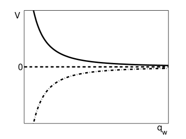
Figure 1: Qualitative plot of the potential $V$ as a function of $q_{w}$ for three cases, $P_{0}<P_{c}$ (solid curve), $P_{0}=P_{c}$ (dashed curve), and $P_{0}>P_{c}$ (dash-dot curve) when $D=2$.

IV.2 The nonlocal case

For the nonlocal case, when $D\leq 2$, the condition (47) can be satisfied automatically. That is to say the (1+1)-dimensional and the (1+2)-dimensional nonlocal solitons are always stable when the response function of the material is a Gaussian function. It is consistent with the conclusion of Ref. Bang-pre-02 . When $D>2$ the solitons can be stable only if the the degree of nonlocality is strong enough that can satisfy the criterion (47), which is also the same as the result of Ref.Bang-pre-02 .

V two remarks

At the end, we make two remarks on the new approach in dealing with the nonlinear light-envelope propagations presented in the paper. Firstly, the new approach is based on the new CEH (23) and (24), and we will show that the conventional CEH (15) and (16) will yield contradictory and inconsistent results. Secondly, we will compare our approach with the variational approach, and discuss the differences between them.

V.1 Contradictory results coming from the conventional CEH

Here we use the conventional CEH (15) and (16) to deal with the light-envelope propagated in nonlinear media, following the same procedure in Sec. IV, and show that the conventional CEH (15) and (16) will give the contradictory and inconsistent results.

Without loss of generality, we only take the NLSE (3) with $D=1$ as an example. The NLSE is a special case of the NNLSE when $w_{m}$ approaches to zero. Then letting $w_{m}=0$ and $D=1$ makes Hamiltonian (33) reduced into

$$H=\frac{\sqrt{\pi}q_{A}^{2}\left[2\sqrt{2}-q_{w}^{2}\left(q_{A}^{2}-2\sqrt{2}q_{w}^{2}q_{c}^{2}\right)\right]}{4q_{w}}.$$ (50)

Because the Hamiltonian is only the function of the generalized coordinates, the CEH (15), the right hand side of which is the derivative of the Hamiltonian with respect to the generalized momentum, can yield nothing unless $\dot{q}_{c}=\dot{q}_{\theta}=\dot{q}_{A}=\dot{q}_{w}=0$. It means the four quantities are all the conserved quantities. This result coming from the CEH (15) is obviously wrong because such quantities as the amplitude $q_{A},$ the width $q_{w}$ and the phase-front curvature $q_{c}$ all generally vary with the evolution coordinate $z$ except for the soliton state, and $q_{\theta}$, the phase of the complex amplitude of the light-envelope, must be the function of $z$ even for the soliton state.

From the other CEH (16), four equations can be obtained as

$$\dot{p}_{c} = -\frac{\partial H}{\partial q_{c}}=-\sqrt{2\pi}q_{A}^{2}q_{c}q_{w}^{3},$$ (51)

$$\dot{p}_{\theta} = -\frac{\partial H}{\partial q_{\theta}}=0,$$ (52)

$$\dot{p}_{A} = -\frac{\partial H}{\partial q_{A}}=\frac{\sqrt{\pi}q_{A}\left(-\sqrt{2}+q_{A}^{2}q_{w}^{2}-\sqrt{2}q_{c}^{2}q_{w}^{4}\right)}{q_{w}},$$ (53)

$$\dot{p}_{w} = -\frac{\partial H}{\partial q_{w}}=\frac{\sqrt{\pi}q_{A}^{2}\left(2\sqrt{2}+q_{A}^{2}q_{w}^{2}-6\sqrt{2}q_{c}^{2}q_{w}^{4}\right)}{4q_{w}^{2}}.$$ (54)

Substitution of the generalized momenta $p_{c}$ given by Eq. (31) into Eq. (51) yields the same result as Eq. (41). Then inserting Eq. (41) into the Hamiltonian (50) gives out $H=\frac{P_{0}}{16}\left(\dot{q}_{w}^{2}+\frac{16}{q_{w}^{2}}-\frac{8P_{0}}{\sqrt{\pi}q_{w}}\right).$ The Hamiltonian is the sum of the generalized kinetic energy and the generalized potential $V(q_{w})=\frac{P_{0}}{2}\left(\frac{2}{q_{w}^{2}}-\frac{P_{0}}{\sqrt{\pi}q_{w}}\right)$, which is also the same as Eq. (43) when $D=1$ and $w_{m}=0$. Therefore, the critical power, corresponding to the extremum point of the generalized potential, $P_{c}=\frac{4\sqrt{\pi}}{q_{w}}$ is the same as Eq. (45) when $D=1$ and $w_{m}=0$. It can also be found that Eq. (52) is the same as Eq. (38), which means that the power of the light-envelope is conservative. Although the first two equations, Eqs. (51) and (52), of a set of equations resulting from CEH (16) can give out the correct results, the other two equations, Eqs. (53) and (54), will yield the contradictory and inconsistent results. Let us show as follows. Inserting Eq. (30) into Eqs.(53) and (54) yields

$$P_{0} = \frac{8\sqrt{\pi}}{5q_{w}},$$ (55)

$$q_{c} = \sqrt{\frac{3}{5}}\frac{1}{q_{w}^{2}}.$$ (56)

Obviously, the two results given by Eqs. (55) and (56) are both wrong. Under the assumption of the light-envelope with the form of Gaussian-shape given by Eq. (27), the power carried by the light-envelope should be $P_{0}=\sqrt{\pi/2}q_{A}^{2}q_{w}$ given by Eq. (39), with which Eq. (55) is contradictory and inconsistent. Eq. (56) gives the fixed relation between $q_{c}$ and $q_{w}$. But the phase-front curvature, $q_{c}$, should be changed depending upon the state of the light-envelope, especially $q_{c}$ should be zero for the soliton state, with which Eq. (56) is inconsistent.

It is no surprise to obtain such contradictory and inconsistent results from the canonical equations of Hamilton (15) and (16), since both the NNLSE (1) and its complex conjugation can not be derived from the canonical equations of Hamilton (17) and (18) as stated in Sec. III.

V.2 Our approach vs the variational approach: same and different

As mentioned above, our approach presented in this paper is based on the canonical equations of Hamilton (the Hamiltonian formulation), while the variational approach Anderson-pra-83 is based on the Euler-Lagrange equations (the Lagrangian formulation). Although the same point of the two approaches is to first compute the Lagrangian of the system by using a suitably chosen trial function, they are in essence two parallel methods because the Hamiltonian formulation and the Lagrangian formulation are two parallel theory frameworks in the classical mechanics.

The most important concept in our approach is the “potential”. The potential given by Eq. (43) is the real “potential” of the system that a single light-envelope propagates in nonlocal nonlinear media modeled by the NNLSE. It is not, of course, the potential of the narrow-sense mechanical system, but does be the potential in the frame of the Hamiltonian theory, that is, the potential of the Hamiltonian system. In other word, it is the potential from the Hamiltonian point of view. Looking back to the variational approach, we can observe that although the “potential” was also introduced [see, Eqs. (28) and (29) in Ref. Anderson-pra-83 ], it is just a mathematically equivalent potential in the sence that the evolution of the width of the light-envelope can be analogous to that of a particle in a potential well, rather than the real “potential” of the system.

VI Conclusion

We introduce a new approach, based on the new canonical equations of Hamilton found by us recently, to analytically obtain the approximate solution of the nonlocal nonlinear Schrödinger equation and to analytically discuss the stability of the soliton. For the single light-envelope propagated in nonlocal nonlinear media modeled by the NNLSE, the Hamiltonian of the system can be constructed as the sum of the generalized kinetic energy and the generalized potential. The extreme point of the generalized potential corresponds to the soliton solution of the NNLSE. The soliton is stable when the generalized potential has the minimum, and unstable otherwise. In addition, we give the rigorous proof of the equivalency between the NNLSE and the Euler-Lagrange equation on the premise of the response function with even symmetry.

References

- (1) G.P. Agrawal, Nonlinear Fiber Optics, 3rd ed. (Acadamic, San Diego, CA, 2001).
- (2) S. Trillo and W. Torruellas, Spatial solitons. (Berlin:Springer-Verlag, 2001).
- (3) Y. S. Kivshar and G. P. Agrawal, Optical Solitons: From Fibers to Photonic Crystals. (New York:Elsevier, 2003).
- (4) G. Assanto, Nematicons: Spatial Optical Solitons in Nematic Liquid Crystals. (New York:John Wiley & Sons, 2012).
- (5) G. I. Stegeman and M. Segev, Science 286, 1518 (1999).
- (6) Z. Chen, M. Segev, and D. N. Christodoulides, Rep. Prog. Phys., 75, 086401 (2012).
- (7) B. A. Malomed et al., J. Opt. B: Quantum Semiclass. Opt., 7, R53 (2005).
- (8) X. Chen, Q. Guo, W. She, H. Zeng, and G. Zhang, Advances in Nonlinear Optics, Chapter 4 (Nonlocal spatial optical solitons), (De Gruyter, Berlin, 2015), p.p.277-306.
- (9) A.W. Snyder and D.J. Mitchell, Science 276, 1538 (1997).
- (10) W. Krolikowski et al., Phys. Rev. E 64, 016612 (2001).
- (11) Q. Guo, W. Hu, D. Deng, et al. Features of strongly nonlocal spatial solitons, Chapter 2 in Nematicons: Spatial Optical Solitons in Nematic Liquid Crystals, edited by G. Assanto. (New York:John Wiley & Sons, 2012).
- (12) Y.S. Kivshar and D.E. Pelinovsky, Phys. Rep. 331, 117 (2000).
- (13) Y. Silberberg, Opt. Lett. , 15, 1282 (1990).
- (14) C. Conti et. al., Phys. Rev. Lett. 105, 263902 (2005); W. Y. Hong, Q. Guo, and L. Li, Phys. Rev. A, submitted for publication.
- (15) V. E. Zakharov and A. B. Shabat, Zh. Eksp. Teor. Fiz. 61, 118 (1971) [Sov. Phys. JETP 34, 62 (1972)].
- (16) V. E. Zakharov and A. B. Shabat, Zh. Eksp. Teor. Fiz. 64, 1627 (1973) [Sov. Phys. JETP 37, 823 (1973)].
- (17) V. I. Karpman and E. M. Maslov, Zh. Eksp. Teor. Fiz. 73, 537 (1977) [Sov. Phys. JETP 46, 281 (1977)].
- (18) Yu. Kivshar and B. A. Malomed, Rev. Mod. Phys. 61, 763 (1989).
- (19) A. I. Maimistov, J. Exp. Theor. Phys. 77, 727 (1993) [Zh. Eksp. Teor. Fiz. 104, 3620 (1993)].
- (20) D. Anderson, Phys. Rev. A27, 3135 (1983).
- (21) B.A. Malomed, in Progress in optics, edited by E. Wolf (North-Holland, 2002), vol.43, pp.71-193.
- (22) Q. Guo, B. Luo, and S. Chi, Opt. Commun. 259, 336 (2006).
- (23) L. Chen, Q. Wang, M. Shen, H. Zhao, Y. Y. Lin, C. C. Jeng, R. K. Lee, and W. Krolikowski, Opt. Lett. 38, 13 (2013).
- (24) H. Steffensen, C. Agger, and O. Bang, J. Opt. Soc. Am. B 29, 484 (2012).
- (25) A. J. Brizard, An Introduction to Lagrangian Mechanics (World Scientific, 2008), formula (1.3), p.3.
- (26) A. J. Brizard, An Introduction to Lagrangian Mechanics (World Scientific, 2008), formula (1.4), p.4.
- (27) H. Goldstein, C. Poole and J. Safko, Classical Mechanics(3rd ed, Addison-Wesley, 2001).
- (28) G. Liang, Z. M. Ren, and Q. Guo, http://arxiv.org/abs/1311.0115, also see, the proceedings of 4th International Conference on Mathematical Modeling in Physical Sciences, June 5-8, 2015, Mykonos, Greece.
- (29) V. Seghete, C.R. Menyuk and B.S. Marks, Phys. Rev. A 76, 043803 (2007).
- (30) A. Picozzi and J. Garnier, Phys. Rev. Lett. 107, 233901 (2011).
- (31) V.M. Lashkin, A.I. Yakimenkoa, and O.O. Prikhodko, Phys. Lett. A 366, 422 (2007).
- (32) M.M. Petroski, M.S. Petrović, M.R. Belić, Opt.Commun. 279,196 (2007).
- (33) N. G. Vakhitov and A. A. Kolokolov, Radiophys. Quantum Electron. 16, 783 (1975).
- (34) To avoid confusion, we make the notations used in Ref.Bang-pre-02 consistent with those in the paper, where we use and to represent the width of the response function and the light-envelope instead of , respectively. In Ref.Bang-pre-02 , , with and , where is the soliton power, and is the propagation constant of solitons. According to the VK criterion, when the soliton become linearly stable. We can derive from the VK criterion , where represents the degree of nonlocality.
- (35) O. Bang, W. Krolikowski, J. Wyller, and J. J. Rasmussen, Phys. Rev. E 66, 046619 (2002).
- (36) M. Desaix, D. Anderson, and M. Lisak, J. Opt. Soc. Am. B8, 2082 (1991).
- (37) L. Berge. Phys. Rep. 303, 259 (1998).
- (38) K. D. Moll, A. L. Gaeta, and G. Fibich, Phys. Rev. Lett. 90 203902 (2003)
- (39) C. Sun, C. Barsi, and J. W. Fleischer, Opt. Express 16 20676 (2008)