Sparse inversion of Stokes profiles

Abstract

Context. Inversion codes are numerical tools used for the inference of physical properties from the observations. Despite their success, the quality of current spectropolarimetric observations and those expected in the near future presents a challenge to current inversion codes.

Aims. The pixel-by-pixel strategy of inverting spectropolarimetric data that we currently utilize needs to be surpassed and improved. The inverted physical parameters have to take into account the spatial correlation that is present in the data and that contains valuable physical information.

Methods. We utilize the concept of sparsity or compressibility to develop an new generation of inversion codes for the Stokes parameters. The inversion code uses numerical optimization techniques based on the idea of proximal algorithms to impose sparsity. In so doing, we allow for the first time to exploit the presence of spatial correlation on the maps of physical parameters. Sparsity also regularizes the solution by reducing the number of unknowns.

Results. We compare the results of the new inversion code with pixel-by-pixel inversions, demonstrating the increase in robustness of the solution. We also show how the method can easily compensate for the effect of the telescope point spread function, producing solutions with an enhanced contrast.

1 Introduction

An inversion code is a computer program based on algorithms that allows the user to extract information about the parameters of a physical system from the interpretation of observables. In solar physics, nonlinear inversion codes are routinely applied after their development in the ’70s to get the thermodynamical and magnetic properties of different regions of the solar atmosphere from the interpretation of the Stokes parameters (Harvey et al. 1972; Auer et al. 1977; Skumanich & Lites 1987).

One of the fundamental problems in general, and specifically for spectropolarimetric inversions, is that the relation between the observables and the physical parameters of interest is very convoluted. Despite the strong nonlinearity and nonlocality inherent to the radiative transfer, it has been possible to develop some simple diagnostics during the past years: the line ratio technique (Stenflo 1973, 2010, 2011), the center-of-gravity method (Semel 1970; Rees & Semel 1979) and calibration curves between spectral line summaries and certain magnetic field properties (e.g., Lites et al. 2008; Martínez Pillet et al. 2011, for recent applications).

The appearance of the first powerful computers allowed researchers to apply optimization techniques for nonlinear functions and use more elaborate models. A $\chi^{2}$ merit function is minimized with respect to the physical parameters defining the specific model. The first efforts (with the application of the computers available at that time) made use of the Milne-Eddington (ME) approximation to analytically solve the radiative transfer equation (e.g., Harvey et al. 1972; Auer et al. 1977; Landi Degl’Innocenti & Landolfi 2004). Although the simplifying assumptions that one needs to use when using the ME approximation may not be fully fulfilled in real solar plasmas, it is still one of the most widely used models, in part because of its simplicity. This simplicity leads to very fast inversion codes that can be applied to the large number of observations that we currently obtain. State-of-the-art inversion codes such as VFISV (Borrero et al. 2007, 2010), used for inferring magnetic field vectors from the Helioseismic and Magnetic Imager (HMI; onboard the Solar Dynamics Observatory) data, MILOS (Orozco Suárez et al. 2007) and MERLIN (Skumanich & Lites 1987; Lites et al. 2007), currently applied to data from the Hinode spacecraft, or the codes based on look-up tables and the principal component analysis (PCA) decomposition (Rees et al. 2000; Socas-Navarro et al. 2001) used for the inversion of THEMIS (Télescope héliographique pour l’étude du magnétisme et des instabilités solaires) data, are based on the ME approximation.

The availability of more powerful computers in recent years allowed us to use more complex and more realistic models. One of the essential ingredients of this revolution was the application of the idea of response functions (Landi Degl’Innocenti & Landi Degl’Innocenti 1977) to the inversion of Stokes profiles with non-trivial depth stratifications of the physical quantities. The first representative of this family of codes was SIR (Stokes Inversion based on Response functions; Ruiz Cobo & del Toro Iniesta 1992). Such evolution occured naturally at that time because observations were showing strong asymmetries in the Stokes profiles in magnetized regions. The explanation of such asymmetries requires the presence of gradients along the line-of-sight (LOS) of the physical properties (Solanki & Pahlke 1988; Grossmann-Doerth et al. 1988; Solanki & Montavon 1993; Sigwarth et al. 1999; López Ariste 2002; Khomenko et al. 2003; Martínez González et al. 2008; Viticchié & Sánchez Almeida 2011). Another representative of these inversions code is SPINOR (Frutiger et al. 2000). Based on the same strategy, Socas-Navarro et al. (2000) developed the NICOLE code (Socas-Navarro et al. 2014), capable of dealing with lines in NLTE (non-local thermodynamical equilibrium). This model has been mainly applied for the inversion of Ca ii infrared triplet lines, which are formed under strong NLTE conditions (e.g., Socas-Navarro et al. 2000; de la Cruz Rodríguez et al. 2012).

Another step forward in the field of inversion codes was carried out by Asensio Ramos et al. (2007) and Asensio Ramos (2009), who introduced Bayesian inference for spectropolarimetric observations. This allows the user to obtain posterior probability distributions for any model parameter and their correlation with the remaining ones. This probabilistic inference is extremely powerful but requires a huge effort in terms of computational power.

Arguably, the latest step in the field of inversion codes has been to compensate the effect of the telescope point spread function (PSF) that is present in the observed data. van Noort (2012) implemented a forward approach, where synthetic spectra from the inversion are convolved spatially with the telescope PSF before comparison with the observations. Ruiz Cobo & Asensio Ramos (2013) used a regularized deconvolution to compensate the observations before the inversions were performed.

The former solves the full problem in which the spatial convolution and the inversion are coupled in the same operator $\mathbf{O}$, resulting in a very large-scale classical inversion code. The use of a Levenberg-Marquardt (LM) scheme (Levenberg 1944; Marquardt 1963) with a compact PSF leads to a sparse Hessian matrix that largely facilitates the inversion by spatially coupling the convergence of adjacent pixels. On the contrary, the latter decouples the inversion. First the observations are deconvolved by applying a PCA regularization in the spectral domain and the application of a standard Richardson-Lucy (Richardson 1972; Lucy 1974) maximum likelihood deconvolution for each eigenimage. Then, the resulting denoised and deconvolved data are inverted using any classical inversion code. Both approaches introduce different regularizations in the inversion problem and can lead to potentially different results.

Also, in the former approach there is no need to consider a low-pass filtering or a regularization of the deconvolution, but the author reports cases of oscillatory patterns in the inferred model that need to be damped during the inversion. In practice, the implementation of the second approach is easier, cleaner and less prone to the aforementioned oscillatory artifacts, but the PCA regularization can filter out features with low statistical weight in the dataset. These methods rely upon accurate knowledge of the PSF used in the inversion, which may not be always available or applicable.

We note that Scharmer et al. (2013) also combined data inversions with a regularized deconvolution to compensate ground-based observations for straylight, believed to originate from small-scale aberrations (Löfdahl & Scharmer 2012).

To take a new step forward in the field of inversion codes, in this paper we propose a new technique to spatially couple the parameters of the model, inspired on the idea of sparsity or compressibility of data. This method allows to use a PSF in the same way as van Noort (2012) but it is not strictly needed for the spatial coupling.

2 Sparsity regularization

With the use of fast slit spectropolarimeters and also two-dimensional filterpolarimeters, we routinely have 2D maps of regions in the solar atmosphere with the four Stokes parameters observed at several points along one or several spectral lines. This rate of new high-quality 2D observations will increase in the future with the advent of bi-dimensional spectropolarimeters based on image slicers or optical fibers. The interpretation of these observations have been done in the past by assuming that all pixels are completely unrelated and applying the inversion codes in a pixel-by-pixel basis. After this pixel-by-pixel inversion, the spatial smoothness of the derived quantities is taken as an indication of the success of the inversions. Salt-and-pepper noise present in the inverted maps of physical parameters is an indication of problems: either the required information cannot be extracted from the Stokes profiles, or the inversions failed to converge to a good solution.

It has become more and more evident that two-dimensional observations and the ensuing inversions are needed to fully understand the physical processes in the solar atmosphere. This is the case even when one assumes local thermodynamical equilibrium (LTE), which relates radiation to the local properties of the plasma. The first representatives of such approach are the already described codes of van Noort (2012) and Ruiz Cobo & Asensio Ramos (2013), where the PSF of the telescope couples the observed Stokes profiles of nearby pixels.

2.1 The general idea

Here we develop the general idea of regularized inversion codes, with the regularization being based on the idea of sparsity. Sparsity or compressibility idealizes the concept that the data can be projected to a parameter space where a reduced set of variables can be used to fully describe that dataset. The motivation for this regularization resides on a very simple observation. When one saves a continuum image as a raw file (for instance, a standard 512$\times$512 pixel image), the size of the file is roughly 1 MB (using 4 bytes per pixel). The same image compressed using a lossless file format reduces the size by a factor 3-4, while a lossy format can go further and increase the compression ratio to a factor $\sim 10$. The compression is possible, fundamentally, due to the existence of spatial correlation (properties like smoothness, structures in the image, …) on the image. If appropriately exploited, it is possible to predict the value of a certain pixel from the values of other pixels thus making it unnecessary to store the value of all pixels.

Let us assume that we have observed the Stokes parameters on a 2D grid of $N_{\mathrm{pix}}=N_{x}\times N_{y}$ pixels for a set of $N_{\lambda}$ wavelength points that sample one or several spectral lines. We propose a model atmosphere for every pixel to explain the observations, each model atmosphere being defined with a set of $N_{\mathrm{par}}$ parameters, so that each pixel $k$ is described with the vector of parameters $\mathbf{\hat{p}}_{k}=(p_{1k},p_{2k},\ldots,p_{N_{\mathrm{par}}k})$. We can build the vector of parameters $\mathbf{p}$ that encode all the model parameters for all the pixels in the field-of-view, such that $\mathbf{\hat{p}}=(\mathbf{\hat{p}}_{1},\mathbf{\hat{p}}_{2},\ldots,\mathbf{\hat{p}}_{N_{\mathrm{pix}}})$. It is possible to reorder this vector so that it is built by stacking the value of each physical parameter for all the pixels, so that $\mathbf{p}=\{\mathbf{p}_{1},\mathbf{p}_{2},\ldots\,\mathbf{p}_{N_{\mathrm{par}}}\}$, where $\mathbf{p}_{i}$ encodes the value of a certain parameter (i.e., magnetic field inclination, Doppler velocity, etc.) as a 2D map. Note that the vectors $\mathbf{p}$ and $\mathbf{\hat{p}}$ are equivalent except for the ordering. The aim of any inversion code is, then, to infer the full vector $\mathbf{p}$ from the observed Stokes profiles. As explained in the introduction, classical inversion codes deal with this problem by inverting the observed Stokes profiles pixel by pixel.

In our approach, instead of working directly on the real space of parameters, we use a linear transformation so that the $i$-th parameter is given by:

$$\mathbf{q}_{i}=\mathbf{W}[\mathbf{p}_{i}].$$ (1)

In the previous equation, $\mathbf{W}$ is a linear operator that transforms from the real space to the transformed space. Among many potential transformations, the most interesting in our context are the Fourier, wavelet or discrete cosine transforms. It is clear that by working on the transformed space and using an inversion code to infer the transformed parameters we have gained nothing. However, here we can impose a fundamental key ingredient: the assumption that the transformed image is sparse in the transformed domain. In other words, if the appropriate transformation $\mathbf{W}$ is used, many elements of the transformed image (that we term modes in the following for simplicity) are zero or very close to zero in absolute value. Sparsity, that is usually fulfilled in nature, has been shown to be an extremely powerful assumption. Techniques like compressed sensing (Candès et al. 2006; Donoho 2006) or exact matrix completion from partial measurements (Candés & Recht 2009) strongly rely on the sparsity assumption.

2.2 Testing for sparsity in physical parameters

For the inversion that we describe in the following to work properly, it is crucial to test for the sparsity of the maps of model parameters. To this end, we do ME pixel-by-pixel inversions of two maps observed with the Solar Optical Telescope/Spectro-Polarimeter SOT/SP (Lites et al. 2001) aboard Hinode (Kosugi et al. 2007). We choose to only invert the Fe i line at 6302.5 Å. The first map is a quiet Sun map extracted from the observations analyzed by Lites et al. (2008), which were obtained at disk center on 2007 March 10. The second map is a sunspot of the active region NOAA 10953, that was mapped at an average heliocentric angle of $\theta=12.8^{\circ}$ on 2007 April 30. This inversion is carried out with a classical inversion code using the LM algorithm and no regularization whatsoever, but the inversion is repeated 10 times for each pixel using different initial values of the model parameters (which are randomized). The ME model depends on a set of assumptions: i) the atmosphere is plane-parallel, semi-infinite, and in local thermodynamic equilibrium, ii) the line opacity, Doppler width, and all line properties are constant with depth on the atmosphere, iii) the magnetic field vector is constant with depth in the atmosphere, and iv) the Planck function is a linear function of the continuum optical depth $\tau_{c}$, so that $B_{T}=B_{0}+B_{1}\tau_{c}$, where $\mathrm{d}\tau_{c}=-\kappa_{c}\mathrm{d}s$, where $\kappa_{c}$ is the continuum opacity. The ME model parameters of our code are: Doppler width of the line in wavelength units ($\Delta\lambda$), macroscopic bulk velocity ($v_{\mathrm{mac}}$), the slope $B_{1}$ and intercept $B_{0}$ of the source function, the ratio between the line and continuum absorption coefficients ($\eta$), the line damping parameter ($a$) and the magnetic field vector parameterized by its modulus, inclination and azimuth with respect to a given reference direction ($B$, $\theta_{B}$ and $\phi_{B}$, respectively).

Figures 1 and 2 display the effect of compressing some parameters in the quiet Sun and the sunspot maps. Both maps contain 256$\times$256 pixels and the selected parameters are the magnetic field strength, Doppler velocity and width of the line. Each panel shows the reconstruction of the original image (the rightmost image in each panel) when the image is transformed using a linear transform, thresholded leaving only a certain percentage of the largest coefficients and transformed back. The percentage of non-zero coefficients is shown as a label in each column. In this example, we use the Daubechies-8 (db8) orthogonal wavelet (Jensen & la Cour-Harbo 2001) as a sparsity enhancing transform, which is appropriate for smooth maps, although the results are similar if other transforms are used. The figure demonstrates that one gets a very well reproduction of the original maps when the number of non-zero coefficients is slightly larger than 15%. This compression can be obtained because the linear transformations capture part of the spatial correlation in the image. As a consequence, the value of $\sim$85% of the pixels can be predicted from the value of just 15% of the image plus the presence of spatial correlation. To help in this comparison, Fig. 3 displays the histogram of the difference between the original magnetic field strength, Doppler velocity and width of the line and the compressed one for different levels of compression. In this case, apart from the Daubechies-8 orthogonal wavelet transform, we also introduce the Haar (db1) orthonormal wavelet (equivalent to the Daubechies-1 wavelet; Jensen & la Cour-Harbo 2001), that is a discontinuous wavelet appropriate for representing efficiently maps with spatial discontinuities and the discrete cosine transform (DCT), appropriate for periodic signals. At the light of these results, keeping 10-15% of the coefficients seems to reproduce very well the original maps of parameters. When the fraction of remaining coefficients is made too small, more artifacts appear and the difference between the original maps and the compressed ones are too large.

Figure 1: Test for the compressibility of the parameters inferred in a quiet Sun map. Each column indicates the number of non-zero coefficients of the original map that are retained.

Figure 2: Same as Fig. 1 but for the sunspot data. We note that these images correspond to the solution of the pixel-by-pixel inversion and contain some artifacts.

Figure 3: Histograms of the difference between the original parameters and the compressed ones at different levels (indicated in each column). The upper panels show the results for the quiet Sun map, while the lower panels refer to the sunspot data. Each histogram refers to a different linear transformation.

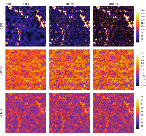
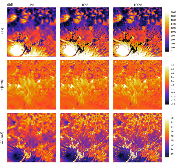
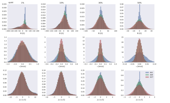
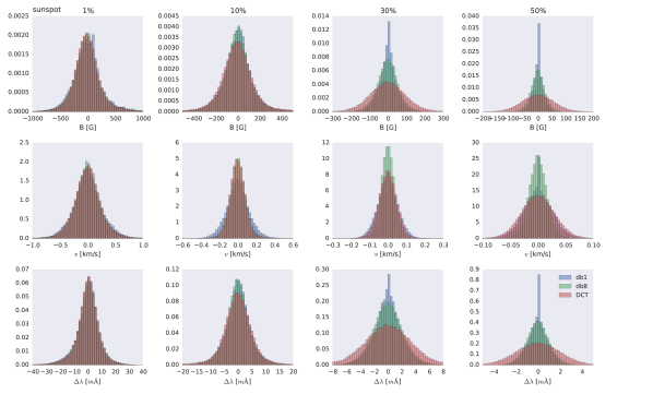
One of the consequences of keeping only a certain percentage of the coefficients in the transformed domain is that we loose some information (lossy compression). It is important that the user of the inversion code described in this paper selects appropriate threshold limits so that no important information is lost in the final maps. Although we recognize the presence of these additional parameters to tweak, standard inversion codes are not easy to use and are also full of parameters to tweak. At the end, all these parameters can be tuned during an initial trial-and-error phase and fixed afterwards.

2.3 Advantages and disadvantages

The inversion code that we describe in the following (together with the numerical techniques needed to enforce sparsity) infers the physical parameters in the transformed space. At the end, the physical parameter of interest is obtained by just a final application of the inverse transform.

Working on the transformed domain and applying a sparsity regularization leads to the following obvious advantages:

• Imposing that the solution to the inversion has to be sparse introduces a strong regularization because the number of unknowns is heavily reduced. From the potential $N_{\mathrm{par}}N_{x}N_{y}$ to only $sN_{\mathrm{par}}N_{x}N_{y}$, with $s\ll 1$. We have found that typical values of the sparsity $s$ will be around 20-30%. Given that a large fraction of the coefficients can be set to zero without degrading the solution, the number of free variables that we are currently using in pixel-by-pixel inversions is highly overestimated. An overly large number of degrees of freedom can produce nonphysical fluctuations of the physical parameters.

• The inverse linear transformation gives the value of a physical parameters at a specific observed pixel as a linear combination of all modes in the map. This global character induces changes in all the pixels of the original space simultaneously when perturbing the value of a single mode. Reversing the argument, the observed Stokes profiles of a single pixel provide a little amount of information to all modes simultaneously. This large redundancy is a very interesting advantage of our approach and introduces a strong regularization of the solution. This global character also introduces strong regularization due to the presence of spatial correlation in the observables and the physical parameters.

The main problem of the method that we present here is that a suitable linear transform has to be chosen a-priori. The wavelet transform is sufficiently versatile so that it can highly compress the 2D maps of many of the physical parameters needed for the synthesis of spectral lines. For this reason, our suggestion is to use the same transform $\mathbf{W}$ for all the parameters. However, the method explained in the following allows the user to choose a different linear operator $\mathbf{W}$ for every parameter $\mathbf{p}_{i}$. This way, it is possible to design a set of linear transforms that leads to a very sparse representation of all the needed physical parameters. This additional step that we need to give as compared with standard pixel-by-pixel inversions is the one that introduces the spatial regularization, though.

2.4 Merit function

All standard inversion codes work by optimizing a merit function that measures the $\ell_{2}$-norm of the residuals with respect to the vector $\mathbf{p}$ of physical parameters. If the observed Stokes parameters are corrupted with Gaussian noise with diagonal covariance matrix, the merit function for the whole map is:

$$\chi^{2}_{\mathbf{p}}=\frac{1}{4N_{\lambda}N_{\mathrm{pix}}}\sum_{k=1}^{N_{\mathrm{pix}}}\sum_{i=1}^{4}\sum_{j=1}^{N_{\lambda}}w_{i}\frac{\left[S_{i}(\lambda_{j},\mathbf{\hat{p}}_{k})-O_{i}(\lambda_{j},k)\right]^{2}}{\sigma_{ijk}^{2}}$$ (2)

where $\mathbf{S}(\lambda_{j},\mathbf{\hat{p}}_{k})=(I(\lambda_{j},\mathbf{\hat{p}}_{k}),Q(\lambda_{j},\mathbf{\hat{p}}_{k}),U(\lambda_{j},\mathbf{\hat{p}}_{k}),V(\lambda_{j},\mathbf{\hat{p}}_{k}))$ refers to the synthetic Stokes vector at wavelength position $j$ and position $k$. Likewise, $\mathbf{O}(\lambda_{j},k)$ is the observed Stokes vector at this very same wavelength and for pixel $k$. The symbol $\sigma_{ijk}$ stands for the standard deviation of the noise at wavelength position $i$, for the Stokes parameter $j$ and pixel $k$, while $w_{i}$ is the weight associated to each Stokes parameter (that we assume, for simplicity, the same for all wavelengths and pixels). This weight is introduced for technical reasons to help improve the convergence during the optimization. Classically, it is customary to solve the problem

$$\operatorname*{arg\,min}_{\mathbf{p}}\,\chi^{2}_{\mathbf{p}},$$ (3)

by direct application of the Levenberg-Marquardt algorithm, which is specially suited to the optimization of such $\ell_{2}$-norms. This involves an optimization for all parameters of all pixels simultaneously. Note that one can indistinguishably use $\mathbf{\hat{p}}$ or $\mathbf{p}$ because the optimization has to be done for all parameters of all pixels.

In a complete parallel formulation, one can work on the transformed domain and write the merit function as:

$$\chi^{2}_{\mathbf{q}}=\frac{1}{4N_{\lambda}N_{\mathrm{pix}}}\sum_{k=1}^{N_{\mathrm{pix}}}\sum_{i=1}^{4}\sum_{j=1}^{N_{\lambda}}w_{i}\frac{\left[S_{i}(\lambda_{j},\left[\mathbf{W}^{-1}[\mathbf{q}]\right]_{k})-O_{i}(\lambda_{j},k)\right]^{2}}{\sigma_{ijk}^{2}}.$$ (4)

The previous expression takes into account that the synthetic Stokes profiles at pixel $k$ depend now on the full vector $\mathbf{q}$ through the linear transformation. Therefore, the inversion problem is solved by computing

$$\operatorname*{arg\,min}_{\mathbf{q}}\,\chi^{2}_{\mathbf{q}}.$$ (5)

The solutions to Eqs. (3) and (5) are strictly equivalent, with the difference that the former is solved in the physical parameters, while the latter in the transformed domain. However, at the light of the results of Figs. 1, 2 and 3, Eq. (5) allows us to impose the sparsity constrain, so that the regularized solution is obtained by computing:

$$\operatorname*{arg\,min}_{\mathbf{q}}\chi^{2}_{\mathbf{q}},\,\,\mathrm{subject\,to\,}\|\mathbf{q}\|_{0}\leq s,$$ (6)

where $\|\mathbf{q}\|_{0}$ is the $\ell_{0}$-norm of $\mathbf{q}$, equivalent to counting the number of non-zero elements. The desired sparsity level is set by the upper limit $s\ll N_{\mathrm{par}}N_{x}N_{y}$. In other words, we minimize the merit function $\chi^{2}$ with respect to the modes $\mathbf{q}$ but using only a very small number of non-zero elements in $\mathbf{q}$. Equivalently, the sparsity constrain can be incorporated in the function through a Lagrange multiplier, so that Eq. (6) can be rewritten as:

$$\operatorname*{arg\,min}_{\mathbf{q}}\chi^{2}_{\mathbf{q}}+\lambda\|\mathbf{q}\|_{0}.$$ (7)

with $\lambda$ a parameter that controls the strength of the constraint.

2.5 Proximal algorithms

As a consequence of the recent huge increase on the interest of compressed sensing, matrix completion, big data and related techniques based on the idea of sparsity, several algorithms have been developed to optimize the addition of convex functions including non-convex constraints ($\ell_{0}$ or $\ell_{1}$ norms, for instance). The objective is to solve the following problem:

$$\operatorname*{arg\,min}_{\mathbf{q}}f(\mathbf{q})+g(\mathbf{q}),$$ (8)

where $f(\mathbf{q})$ is a convex and differentiable function, while $g(\mathbf{q})$ is another convex function, possible non-smooth. This is exactly the type of problem that we have to solve in Eq. (7), in our case with $f(\mathbf{q})=\chi^{2}_{\mathbf{q}}$ and $g(\mathbf{q})=\lambda\|\mathbf{q}\|_{0}$.

One of the most successful algorithms developed recently belong to the class of methods termed proximal algorithms (e.g., Parikh & Boyd 2014). They can be viewed as the equivalent of the Newton method for non-smooth, constrained, and large-scale optimization problems. In this case, the solution to the general problem (8) is given by the following iteration (e.g., Starck et al. 2010):

$$\mathbf{q}_{i+1}=\mathrm{prox}_{g}\left[\mathbf{q}_{i}-\mathbf{h}\nabla_{\mathbf{q}}f(\mathbf{q}_{i})\right],$$ (9)

where one carries out a step along the gradient of $f(\mathbf{q})$ and then applies the so-called proximity operator, defined in the following. Note that, since $f(\mathbf{q})=\chi^{2}_{\mathbf{q}}$ is differentiable, the term inside parenthesis is the standard gradient descent method that are typically used in many inversion codes for the Stokes parameters.

It is clear from Eq. (9) that the key ingredient of these proximal algorithms is the application of the proximity operator of the regularization function $g(\mathbf{x})$, defined as (Parikh & Boyd 2014):

$$\mathrm{prox}_{g}(\mathbf{x})=\operatorname*{arg\,min}_{\mathbf{v}}\left[\frac{1}{2}\|\mathbf{v}-\mathbf{x}\|_{2}^{2}+\lambda g(\mathbf{v})\right].$$ (10)

In general, this proximal operator has to be computed numerically, but exact solutions exist for many interesting regularization terms (Parikh & Boyd 2014). In fact, in our case that we use the $\ell_{0}$-norm as regularization, the proximity operator is simply given by:

$$\mathrm{prox}_{\ell_{0}}(\mathbf{x})=H_{s}(\mathbf{x}),$$ (11)

where $H_{s}(\mathbf{x})$ is the nonlinear hard thresholding operator. This operator keeps the $s$ elements of $\mathbf{x}$ with largest absolute value untouched and sets to zero the remaining elements. Although all the results presented in this paper use the $\ell_{0}$-norm as regularization, sometimes it is interesting to use the $\ell_{1}$-norm. In this case, the proximal operator is the smooth thresholding operator, which is given by:

$$\mathrm{prox}_{\ell_{1}}(\mathbf{x})=\mathrm{sign}(\mathbf{x})(|\mathbf{x}|-\lambda)_{+},$$ (12)

where $(\cdot)_{+}$ denotes the positive part.

Data: Stokes profiles and model atmosphere

Result: $\ell_{0}$-regularized solution

Initialization: $t_{0}=1$ and $\mathbf{y}_{1}=\mathbf{q}_{0}$, with $\mathbf{q}_{0}$ a first estimation of the modes;

while not converged do

       $\mathbf{q}_{k}=H_{s}\left[\mathbf{y}_{k}-\mathbf{h}\nabla_{\mathbf{q}}\chi^{2}(\mathbf{y}_{k})\right]$;

       $t_{k+1}=\frac{1+\sqrt{1+4t_{k}^{2}}}{2}$;

       $\mathbf{y}_{k+1}=\mathbf{q}_{k}+\left(\frac{t_{k}-1}{t_{k+1}}\right)(\mathbf{q}_{k}-\mathbf{q}_{k-1})$;

       if $\nabla_{\mathbf{q}}\chi^{2}(\mathbf{y}_{k})(\mathbf{q}_{k}-\mathbf{q}_{k-1})>0$ then

             $\mathbf{q}_{0}=\mathbf{y}_{0}=\mathbf{x}_{k}$, $t_{k}=1$ and $k=0$;

            

       end if

      

end while

return $\mathbf{q}_{k}$

Algorithm 1 FISTA algorithm with restarting strategy.

Putting together Eqs. (9) and (11), the simplest proximal algorithm that uses the gradient descent method to solve Eq. (7) is given by (e.g., Parikh & Boyd 2014):

$$\mathbf{q}_{k+1}=H_{s}\left[\mathbf{q}_{k}-\mathbf{h}\nabla_{\mathbf{q}}\chi^{2}(\mathbf{q}_{k})\right].$$ (13)

This iteration is just a plain gradient descent algorithm (which only makes use of first order derivatives) which is augmented by using a hard thresholding projection operator in each iteration. In other words, after moving the solution on the direction of the negative gradient (controlled by the step-size $\mathbf{h}$), one sets to zero all elements that do not fulfill the sparsity constraint. This simple iterative scheme displays a sublinear convergence rate $O(1/k)$. Recently, a trivial improvement of the gradient descent method known as Fast Iterative Shrinkage-Thresholding Algorithm (FISTA) has been developed by Beck & Teboulle (2009) showing a quadratic convergence rate $O(1/k^{2})$. Algorithm 1, a combination of FISTA and the restarting scheme developed by O’Donoghue & Candès (2012), is our method of choice in this paper. We leave for the future the analysis of algorithms that smartly introduce some second-order information without ever constructing the Hessian matrix (e.g., Becker & Fadili 2012).

Eq. (13) shows that the optimization method relies on the computation of the gradient of the merit function with respect to the modes $\mathbf{q}$, that we have made explicity by using the subindex $\mathbf{q}$ on $\nabla_{\mathbf{q}}\chi^{2}$. Given the linear character of the transformation of Eq. (1), this gradient can be trivially related to the gradient with respect to the physical parameters (the response functions), that can be analitically written as:

$$\nabla_{\mathbf{q}_{i}}\chi^{2}=\mathbf{W}^{-1}\nabla_{\mathbf{p}_{i}}\chi^{2},\qquad i=1,\ldots,N_{\mathrm{par}}.$$ (14)

The method described in this section is independent of the specific details of the transform $\mathbf{W}$. The only condition is that it has to be linear and invertible. Apart from that, it is also desirable from the computational point of view that the linear transform has a fast algorithm available. This is the case both for the orthogonal wavelet and DCT transforms.

2.6 Possible improvements

Even though gradient descent methods are known to be fast when approaching the minimum, they become slower in the refinement phase of the solution (that is precisely the reason why the Levenberg-Marquardt method is a combination of a gradient descent method and a Newton method, controlled by the Hessian). However, the non-convex optimization of large-scale problems has to rely on first-order derivatives because the calculation and storage of the Hessian is impractical. In our experience and that of many others in the literature, the FISTA algorithm is a competitive optimization technique. To achieve a good convergence speed, the vector of step-sizes $\mathbf{h}$ has to be smartly chosen. Extensive experiments have convinced us that these steps can be kept fixed and used in different data sets without any special impact on the convergence speed. However, we are currently investigating the possibility of improving the convergence speed along two lines. First, using approximations to the diagonal Hessian matrix that can be efficiently computed using quasi-Newton methods. Quasi-Newton methods update the Hessian matrix by analyzing successive gradient vectors using a generalization of the secant method. We anticipate that the methods developed by Becker & Fadili (2012) or Marjugi & Leong (2013) can be of help. Second, using conjugate gradient methods.

We have noticed that convergence is greatly improved if the inversion is started forcing a very sparse solution, which in practice is similar to reducing the number of parameters in the first steps (Ruiz Cobo & del Toro Iniesta 1992). Once the model cannot be further improved, the inversion can be re-started assuming the final target sparsity, and therefore, giving more freedom to the inversion in the final steps. In fact, we have noticed that in cases where the sparsity is assumed to be low, the inversion can get stuck when $\chi^{2}$ is still very high. We blame the FISTA algorithm with fixed $\mathbf{h}$ for this behaviour. We expect to ameliorate this behaviour with the future improvements that are described above.

Figure 4: Inverted maps for some of the most relevant physical parameters of the model for a quiet Sun observation. The map is 512$\times$512 pixels. The left column shows the pixel-by-pixel results, while the central panels display the results of the sparsity regularized inversion, using a Daubechies-8 orthogonal wavelet and a thresholding value of 50%. The third column corresponds to a sparsity regularized inversion compensating for the Hinode telescope PSF.

2.7 Summary

The inversion scheme that we propose in this paper works as follows. A linear transform is chosen so that the transformed 2D maps of model parameters are as sparse as possible. We have tested that DCT and wavelet transforms seem to be appropriate. At the beginning of the iterative process, all the model parameters are initialized using any appropriate initialization like any standard inversion code. The initial solution is transformed to obtain the first estimation of the modes. At each iteration, the value of the merit function and of its gradient with respect to the model parameters taking into account all observed pixels are computed. To this end, the inverse transform of the current solution has to be computed. The gradients, reordered as 2D maps, are transformed using Eq. (14). Once the gradient descent step is applied, the sparsity constrain is applied by hard thresholding the resulting new modes. In this somehow trivial step is where the sparsity condition is applied. Finally, algorithm 1 is repeated until convergence.

3 The computer code

We have developed a computer code using the ideas presented in the previous section. The code is written in C++ using the Message Passing Interface (MPI) standard for parallelization using a master-slave strategy. One node works as a master, sending calculations to the slaves and receiving the results. Although the architecture of the code is very general, the current version of the code only works with the ME model atmosphere. It can be used to carry out pixel-by-pixel inversions (using the LM algorithm) and also sparsity regularized two-dimensional inversions (using the FISTA algorithm). We will provide extensive details on the implementation in a near future, once the code is expanded to use more realistic cases than the ME included in this paper (de la Cruz Rodríguez et al. in prep.). Additionally, we will make the code freely available.

Figure 5: Value of the $\chi^{2}$ for each Stokes parameter for the pixel-by-pixel inversion (left panels) and the sparsity regularized inversion (right panels).

The code starts by using an initial estimation of the transformed coefficients for the maps of parameters. With this initialization, the computationally heavy part of the calculation of the $\chi^{2}$ and the gradient term $\nabla_{\mathbf{p}}\chi^{2}$ is fully parallelized, with each slave working on a piece of the map. When all the information is gathered by the master node, it computes the gradient term in the transformed domain by direct application of Eq. (14). This are the needed quantities to evaluate one iteration of the FISTA algorithm and produce a correction of the transformed coefficients of the maps of physical quantities. This very same procedure is iterated until convergence.

The code also allows the user to specify a PSF that is used for degrading the synthetic profiles and carry out the spatial deconvolution and the regularized inversion simultaneously, similar to the approach followed by van Noort (2012). The inclusion of the deconvolution is straightforward in our first-order approach. The convolution operator is linear so that, apart from convolving the Stokes profiles with the PSF, we only need to convolve the response functions with the PSF, so that Eq. (14) becomes

$$\nabla_{\mathbf{q}_{i}}\chi^{2}=\mathbf{P}\ast\left[\mathbf{W}^{-1}\nabla_{\mathbf{p}_{i}}\chi^{2}\right],\qquad i=1,\ldots,N_{\mathrm{par}}$$ (15)

where $\ast$ is the convolution operator.

Figure 6: Same as Fig. 4 but for the sunspot data.

4 Illustrative examples

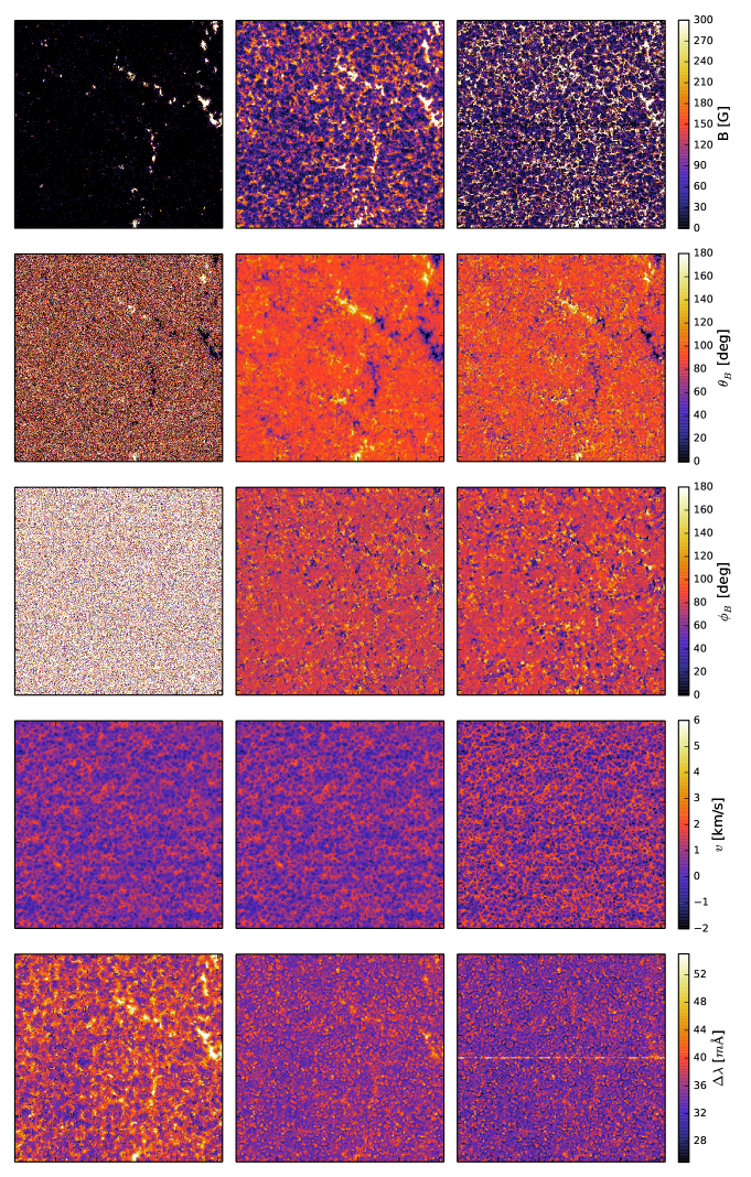
As a demonstration of our approach, we present in Fig. 4 the inverted maps for some physical parameters of the ME model in the quiet Sun map. Since the inversion is carried out with a very simple model with only one component that is not able to capture the behavior of unresolved fields, we cannot infer much from the magnetic properties on the map. However, a few things need to be commented:

1. The pixel-to-pixel inversion has been carried out in a multistep process to improve the quality of the fit. First, we obtained a result from 50 randomizations of the initial parameters, keeping only the best solution for each pixel. Then we smooth the map with a Gaussian kernel. Finally, we re-run the inversion with another 50 randomizations, starting from the smoothed maps. We keep the solution that produces the best fit.

2. The general appearance of the maps is much cleaner for the sparsity regularized maps, a consequence of the thresholding. This avoids arbitrary pixel-to-pixel variations because some spatial coherence is forced.

3. The map of Doppler velocities are indistinguishable for the two inversions, meaning that this quantity is very easy to find in a pixel-by-pixel inversion.

4. The spatially regularized inversion returns lots of fields inclined by $\sim$90^∘. This is a direct consequence of the fact that many pixels have very low signal-to-noise ratio (SNR). The bias produced by the noise on the transversal component of the magnetic field (Martínez González et al. 2012) makes that the fields systematically appear very inclined.

5. We also find that the Doppler width of the line is larger in the granules than in the intergranules on the sparsity regularized solution. The opposite is found in the pixel-by-pixel inversion. This behavior is compensated in the sparsity regularized solution by an small increase of the magnetic field.

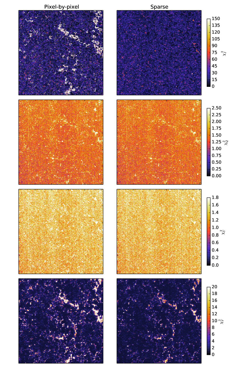
6. The maps in the third column of Fig. 4 show the effect of compensating for the telescope PSF. Features become more conspicuous and compact, as demonstrated by van Noort (2012) and Ruiz Cobo & Asensio Ramos (2013).

The quality of the fits is assessed by computing the associated $\chi^{2}$ for each Stokes parameter and shown in Fig. 5. Curiously, the sparsity regularized inversion is comparable for Stokes $Q$, $U$ and $V$ and much better for Stokes $I$, because the sparse solution does not show all the structuring visible in the pixel-by-pixel one. This demonstrates that our inversion code finds a much simpler model (in terms of the number of free parameters) that explains the data better.

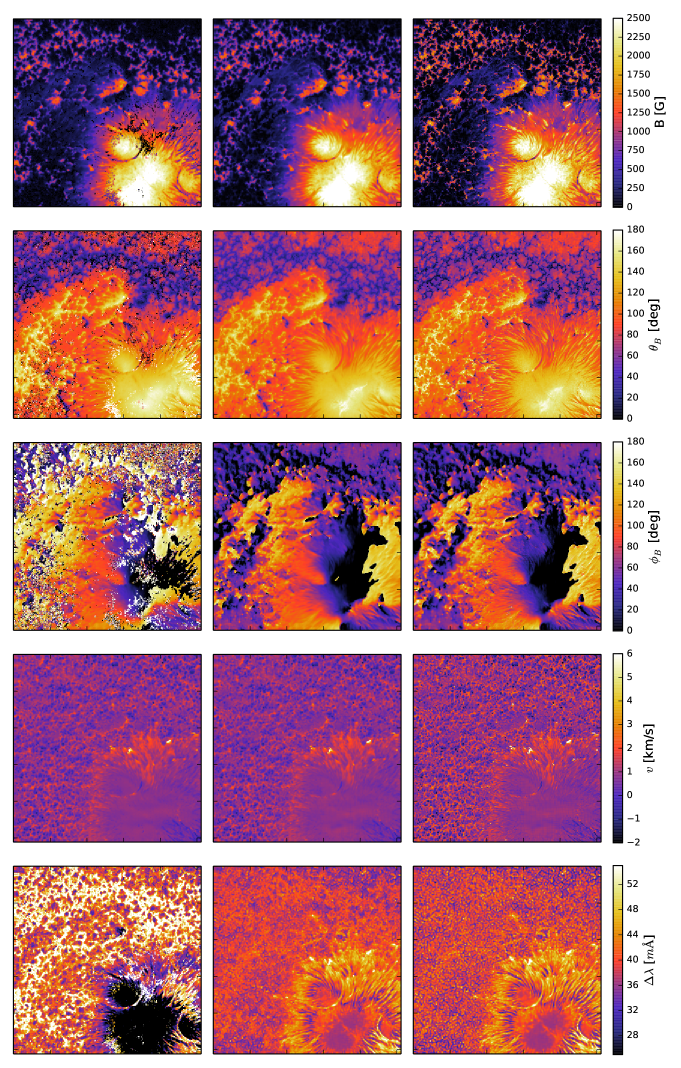
Figure 6 shows the results for the sunspot data. Again, the inferred Doppler velocities are very similar in the two approaches, giving robustness to this quantity. The same behavior is also seen in the Doppler width of the line, with granules presenting spectral lines with an enhanced broadening as compared with the intergranular lanes. The same applies to the penumbra, where we find dark filaments to have a smaller Doppler width. Concerning the magnetic field vector, we find smoother smoother and much less noisy results.

Figure 7: Convergence of $\chi^{2}$ as a function of iteration number for the two data sets.

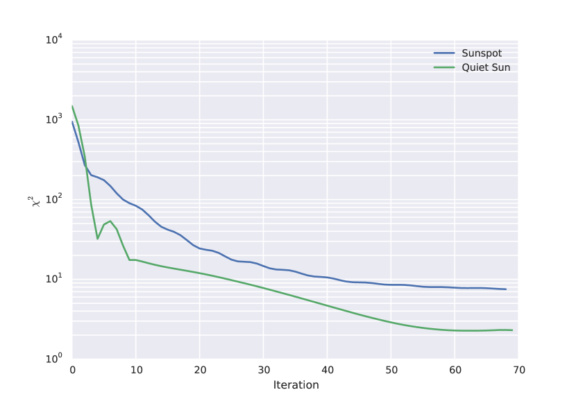
Concerning the convergence speed, Fig. 7 displays the value of the reduced $\chi^{2}$ in the whole map and taking into account all Stokes parameters for the two datasets. As usual in first-order, the initial convergence is very fast, while the refinement of the solution is slower. We note that artifacts can appear in the sparse inversion when the solution is not fully converged. Unlike the pixel-by-pixel case, these artifacts appear as spatially coherent patches in the solution, that deviate from the surroundings. When the solution is converged, these patches disappear. Therefore, a different intuition is needed to assess whether the solution is physically meaningful or not.

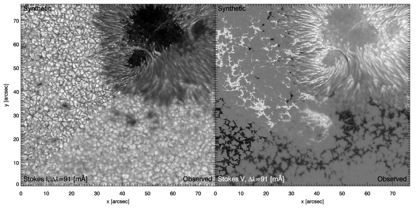
Finally, Fig. 8 illustrates the smearing effect of the PSF in the observed data. We have not noticed the oscillatory behavior that was reported by van Noort (2012). We speculate that the regularization present in our sparse inversion naturally damps that behavior, but to be fair a ME model is simpler than the depth-dependent case consider by van Noort (2012) and this issue should be addressed under the same conditions.

5 Conclusion and outlook for the future

This paper presents the first full 2D regularized inversion code for Stokes profiles based on the idea of sparsity. Although the atmosphere model that we use is very simple, it represents the first step toward a full suite of inversion codes. The strong spatial regularization that we introduce thanks to the sparsity constrain allows us to obtain very reliable results.

Figure 8: Illustration of the effect of the telescope PSF in the data. The FOV is divided in two halfs for a monochromatic image at $\Delta\lambda=91$ mÅ from line center in Stokes $I$ (left) and $V$ (right). The lower half shows the observations, without applying the PSF compensation. The upper half shows the synthetic image from the inversion, including the PSF compensation. This inversion has been performed assuming $50\%$ sparsity.

Our method is built upon some of the ideas presented by van Noort (2012) and Ruiz Cobo & Asensio Ramos (2013): the model is spatially coupled and regularized. Furthermore, given that we do not use a Hessian based inversion method, compensating the data for telescope or stray-light PSF is trivial, as it does not add extra complexity to the code, beyond the actual computation of convolutions. However, if the telescope PSF is not known, the sparse regularization will also couple the parameters from neighboring pixels. The intrinsic nature of the wavelet transform allows to reproduce small-scale and localized features, as well as the large scales and therefore, reducing the number of free parameters does not necessarily preclude the code from reproducing gradients and sharp features if the correct sparsity level is chosen.

In this study we have used the first-order accelerated FISTA optimization algorithm to perform the 2D sparse inversion. We emphasize that we are exploring alternative methods to further improve the convergence of the inversion.

A fast and parallel inversion code implementing everything that is presented in this work and some extensions as described in the following will be freely available for the community soon. The code will be extensible if the user provides the emergent Stokes profiles from a given parameterized atmosphere and the response function of the Stokes parameters to all parameters. This response function can be computed analytically or, in general, numerically.

The concept of sparse regularization can be extended to many other problems that we plan to analyze in this series of papers, not necessarily maintaining the order. In a first step, we plan to extend the sparse regularization to atmospheres with gradients in the vertical direction. This will be done by fixing a set of heights in a common optical depth scale (for instance, the optical depth scale at 500 nm) that will play the role of nodes, in parallel to which is currently done in standard inversion codes like SIR, Nicole or SPINOR. The physical parameters (temperature, velocity, magnetic field, etc.) at each node will be assumed to be sparse in a wavelet basis and the strategy used in this paper will be applied to fit the emergent Stokes profiles.

In a second step, the concept of nodes will be surpassed. Each physical parameter will be determined by a 3D cube that will be assumed to be sparse in a three-dimensional basis (DCT and orthogonal wavelets are trivially extended to the three dimensional case). Therefore, the inversion will proceed by inferring a reduced number of wavelet modes for each physical parameter. The regularization imposed in this 3D inversion is very strong because the observation of a single pixel provides (probably little) information for constraining the depth stratification of all the pixels in the cube.

In a third step, standard pixel-by-pixel inversions can be carried out using a sparse regularization in height. The concept of nodes, that have been present in all inversion codes with depth stratification looses its meaning again. The depth stratification of the physical parameters of interest will be expanded in a suitable dictionary of depth-dependent functions (we use the term dictionary because the functions do not need, in principle, to be orthogonal) and the optimization will select the smallest number of functions needed to reproduce the Stokes profiles.

Finally, we note that our strategy could potentially be extended to do regularized superresolution. We leave this analysis for the future because it needs to be studied in detail.