1 Introduction
Suppose that we have independent observations x β ( 1 ) , x β ( 2 ) , β¦ , x β ( N ) π₯ 1 π₯ 2 β¦ π₯ π
x(1),x(2),\ldots,x(N) from
a probability density p β ( x β£ ΞΈ ) π conditional π₯ π p(x\mid\theta) that belongs to a parametric model { p β ( x β£ ΞΈ ) β£ ΞΈ β Ξ } conditional π conditional π₯ π π Ξ \{p(x\mid\theta)\mid\theta\in\Theta\} ,
where ΞΈ = ( ΞΈ 1 , ΞΈ 2 , β¦ , ΞΈ d ) π superscript π 1 superscript π 2 β¦ superscript π π \theta=(\theta^{1},\theta^{2},\ldots,\theta^{d}) is an unknown d π d -dimensional parameter and Ξ Ξ \Theta is the parameter space.
The random variable y π¦ y to be predicted is independently distributed according to
a density p ~ β ( y β£ ΞΈ ) ~ π conditional π¦ π \displaystyle\tilde{p}(y\mid\theta) in a parametric model { p ~ β ( y β£ ΞΈ ) β£ ΞΈ β Ξ } conditional ~ π conditional π¦ π π Ξ \{\displaystyle\tilde{p}(y\mid\theta)\mid\theta\in\Theta\} ,
possibly different from { p β ( x β£ ΞΈ ) β£ ΞΈ β Ξ } conditional π conditional π₯ π π Ξ \{p(x\mid\theta)\mid\theta\in\Theta\} ,
with the same parameter ΞΈ π \theta .
The objective is to construct a predictive density p ^ β ( y ; x N ) ^ π π¦ superscript π₯ π
\hat{p}(y;x^{N}) for y π¦ y by using x N := ( x β ( 1 ) , β¦ , x β ( N ) ) assign superscript π₯ π π₯ 1 β¦ π₯ π x^{N}:=(x(1),\ldots,x(N)) .
The performance of p ^ β ( y ; x ) ^ π π¦ π₯
\hat{p}(y;x) is evaluated by the KullbackβLeibler divergence
D β ( p ~ β ( y β£ ΞΈ ) , p ^ β ( y ; x N ) ) := β« p ~ β ( y β£ ΞΈ ) β log β‘ p ~ β ( y β£ ΞΈ ) p ^ β ( y ; x N ) β d β y assign π· ~ π conditional π¦ π ^ π π¦ superscript π₯ π
~ π conditional π¦ π ~ π conditional π¦ π ^ π π¦ superscript π₯ π
d π¦ D(\displaystyle\tilde{p}(y\mid\theta),\hat{p}(y;x^{N})):=\int\displaystyle\tilde{p}(y\mid\theta)\log\frac{\displaystyle\tilde{p}(y\mid\theta)}{\hat{p}(y;x^{N})}\mbox{d}y\
from the true density p ~ β ( y β£ ΞΈ ) ~ π conditional π¦ π \displaystyle\tilde{p}(y\mid\theta) to the predictive density p ^ β ( y ; x N ) ^ π π¦ superscript π₯ π
\hat{p}(y;x^{N}) .
The risk function is given by
E β [ D β ( p ~ β ( y β£ ΞΈ ) , p ^ β ( y ; x N ) ) | ΞΈ ] = β¬ p β ( x N β£ ΞΈ ) β p ~ β ( y β£ ΞΈ ) β log β‘ p ~ β ( y β£ ΞΈ ) p ^ β ( y ; x N ) β d β y β d β x N . E delimited-[] conditional π· ~ π conditional π¦ π ^ π π¦ superscript π₯ π
π double-integral π conditional superscript π₯ π π ~ π conditional π¦ π ~ π conditional π¦ π ^ π π¦ superscript π₯ π
d π¦ d superscript π₯ π {\rm E}\Bigl{[}D(\displaystyle\tilde{p}(y\mid\theta),\hat{p}(y;x^{N}))\,\Big{|}\,\theta\Bigr{]}=\iint p(x^{N}\mid\theta)\displaystyle\tilde{p}(y\mid\theta)\log\frac{\displaystyle\tilde{p}(y\mid\theta)}{\hat{p}(y;x^{N})}\mbox{d}y\mbox{d}x^{N}.
It is widely recognized that
plug-in densities p ~ β ( y β£ ΞΈ ^ ) ~ π conditional π¦ ^ π \displaystyle\tilde{p}(y\mid\hat{\theta}) constructed by replacing the unknown parameter ΞΈ π \theta
by an estimate ΞΈ ^ β ( x N ) ^ π superscript π₯ π \hat{\theta}(x^{N})
may not perform very well
and that Bayesian predictive densities
p ~ Ο β ( y β£ x N ) := β« p ~ β ( y β£ ΞΈ ) β p β ( x N β£ ΞΈ ) β Ο β ( ΞΈ ) β d β ΞΈ β« p β ( x N β£ ΞΈ ) β Ο β ( ΞΈ ) β d β ΞΈ assign subscript ~ π π conditional π¦ superscript π₯ π ~ π conditional π¦ π π conditional superscript π₯ π π π π d π π conditional superscript π₯ π π π π d π \displaystyle\tilde{p}_{\pi}(y\mid x^{N}):=\frac{\int\displaystyle\tilde{p}(y\mid\theta)p(x^{N}\mid\theta)\pi(\theta)\mbox{d}\theta}{\int p(x^{N}\mid\theta)\pi(\theta)\mbox{d}\theta}
constructed by using a prior Ο π \pi perform better than plug-in densities.
If the value of ΞΈ π \theta is given, there is no specific meaning of considering the conditional
density of y π¦ y given x N superscript π₯ π x^{N} since the obvious relation
p β ( y β£ x , ΞΈ ) = p β ( y β£ ΞΈ ) π conditional π¦ π₯ π
π conditional π¦ π p(y\mid x,\theta)=p(y\mid\theta) holds.
However, if ΞΈ π \theta is unknown, Bayesian predictive densities p Ο β ( y β£ x N ) subscript π π conditional π¦ superscript π₯ π p_{\pi}(y\mid x^{N})
constructed by introducing a prior density Ο β ( ΞΈ ) π π \pi(\theta) on the parameter space are useful
to approximate the true density p β ( y β£ ΞΈ ) π conditional π¦ π p(y\mid\theta) as discussed in Aitchison and Dunsmore (1975 ) and Geisser (1993 ) .
In fact, there exists a predictive density whose asymptotic risk is smaller than
that of a plug-in density unless the mean mixture curvature of the model
manifold vanishes, see Komaki (1996 ) and Hartigan (1998 ) for details.
The choice of Ο π \pi becomes important especially when the sample size N π N is not very large.
Although the Jeffreys prior is a widely known default prior,
it does not perform satisfactorily especially when the unknown parameter is multidimensional as Jeffreys himself
pointed out.
Komaki (2001 ) constructed a Bayesian predictive density incorporating the advantage of
shrinkage methods for the multivariate normal model.
See also George etΒ al. (2006 ) for useful results for the normal model.
In the conventional setting in which the distributions of x β ( i ) π₯ π x(i) , i = 1 , β¦ , N π 1 β¦ π
i=1,\ldots,N , and y π¦ y are the same,
asymptotic theory of prediction based on general parametric models has been studied
by using the framework of information geometry, see Komaki (1996 ) .
In information geometry, a parametric statistical model is regarded as a differentiable manifold,
which we call the model manifold, and the parameter space
is regarded as a coordinate system of the manifold, see Amari (1985 ) .
The FisherβRao metric is
a Riemannian metric based on the Fisher information matrix on the model manifold.
The Jeffreys prior Ο J β ( ΞΈ ) subscript π J π \pi_{\mathrm{J}}(\theta) corresponds to the volume element of the model manifold associated with the FisherβRao metric.
When the distributions of x β ( i ) π₯ π x(i) , i = 1 , β¦ , N π 1 β¦ π
i=1,\ldots,N , and y π¦ y are the same,
the asymptotic difference between the risks of p ~ Ο β ( y β£ x N ) subscript ~ π π conditional π¦ superscript π₯ π \displaystyle\tilde{p}_{\pi}(y\mid x^{N}) and p ~ J β ( y β£ x N ) subscript ~ π J conditional π¦ superscript π₯ π \displaystyle\tilde{p}_{\mathrm{J}}(y\mid x^{N}) is given by
N 2 [ E { \displaystyle N^{2}\biggl{[}{\rm E}\big{\{}
D ( p ~ ( y β£ ΞΈ ) , p ~ Ο ( y β£ x N ) | ΞΈ } β E { D ( p ~ ( y β£ ΞΈ ) , p ~ J ( y β£ x N ) | ΞΈ } ] \displaystyle D(\displaystyle\tilde{p}(y\mid\theta),\displaystyle\tilde{p}_{\pi}(y\mid x^{N})\,\big{|}\,\theta\big{\}}-{\rm E}\big{\{}D(\displaystyle\tilde{p}(y\mid\theta),\displaystyle\tilde{p}_{\mathrm{J}}(y\mid x^{N})\,\big{|}\,\theta\big{\}}\biggr{]}
= \displaystyle=
Ξ β ( Ο Ο J ) ( Ο Ο J ) β 1 2 β β i = 1 d β j = 1 d g i β j β β i ( Ο Ο J ) β β j ( Ο Ο J ) ( Ο Ο J ) 2 + o β ( 1 ) = 2 β Ξ β ( Ο Ο J ) 1 2 ( Ο Ο J ) 1 2 + o β ( 1 ) , Ξ π subscript π J π subscript π J 1 2 superscript subscript π 1 π superscript subscript π 1 π superscript π π π subscript π π subscript π J subscript π π subscript π J superscript π subscript π J 2 o 1 2 Ξ superscript π subscript π J 1 2 superscript π subscript π J 1 2 o 1 \displaystyle\frac{\displaystyle\Delta\left(\frac{\pi}{\pi_{\mathrm{J}}}\right)}{\displaystyle\left(\frac{\pi}{\pi_{\mathrm{J}}}\right)}-\frac{1}{2}\sum_{i=1}^{d}\sum_{j=1}^{d}g^{ij}\frac{\displaystyle\partial_{i}\left(\frac{\pi}{\pi_{\mathrm{J}}}\right)\partial_{j}\left(\frac{\pi}{\pi_{\mathrm{J}}}\right)}{\displaystyle\left(\frac{\pi}{\pi_{\mathrm{J}}}\right)^{2}}+\mathrm{o}(1)=2\frac{\displaystyle\Delta\left(\frac{\pi}{\pi_{\mathrm{J}}}\right)^{\frac{1}{2}}}{\displaystyle\left(\frac{\pi}{\pi_{\mathrm{J}}}\right)^{\frac{1}{2}}}+\mathrm{o}(1),
(1)
where
β i subscript π \partial_{i} denotes β / β ΞΈ i superscript π π \partial/\partial\theta^{i} ,
g i β j := E β { β i log β‘ p β ( x β£ ΞΈ ) β β j log β‘ p β ( x β£ ΞΈ ) β£ ΞΈ } assign subscript π π π E conditional subscript π π conditional π₯ π subscript π π conditional π₯ π π g_{ij}:={\rm E}\{\partial_{i}\log p(x\mid\theta)\partial_{j}\log p(x\mid\theta)\mid\theta\} ,
g i β j superscript π π π g^{ij} denotes the ( i , j ) π π (i,j) -element of the inverse of the d Γ d π π d\times d matrix ( g i β j ) subscript π π π (g_{ij}) ,
and Ξ Ξ \Delta is the Laplacian, see Komaki (2006 ) .
The Laplacian Ξ Ξ \Delta on a Riemannian manifold endowed with a metric g i β j subscript π π π g_{ij} is defined by
Ξ β f = | g | β 1 / 2 β β i β j β i ( | g | 1 / 2 β g i β j β β j f ) = β i β j β i ( 0 ) ( g i β j β β j f ) , Ξ π superscript π 1 2 subscript π subscript π subscript π superscript π 1 2 superscript π π π subscript π π subscript π subscript π superscript subscript β π 0 superscript π π π subscript π π \displaystyle\Delta f=|g|^{-1/2}\sum_{i}\sum_{j}\partial_{i}(|g|^{1/2}g^{ij}\partial_{j}f)=\sum_{i}\sum_{j}\nabla_{i}^{(0)}(g^{ij}\partial_{j}f),
(2)
where | g | π |g| is the determinant of the d Γ d π π d\times d matrix ( g i β j ) subscript π π π (g_{ij}) ,
f π f is a smooth real function on Ξ Ξ \Theta , and β i ( 0 ) superscript subscript β π 0 \nabla_{i}^{(0)} denotes
the covariant derivative, defined in the next section.
The indices i , j , k β β¦ π π π β¦
i,j,k\ldots run from 1 1 1 to d π d .
Note that both the definition (2 ) of the Laplacian
and the definition Ξ β f = β | g | β 1 / 2 β β i β j β i ( | g | 1 / 2 β g i β j β β j f ) Ξ π superscript π 1 2 subscript π subscript π subscript π superscript π 1 2 superscript π π π subscript π π \Delta f=-|g|^{-1/2}\sum_{i}\sum_{j}\partial_{i}(|g|^{1/2}g^{ij}\partial_{j}f) that differs in sign
are widely adopted in the mathematics literature,
although it is confusing.
Because of (1 ), if there exists a non-constant positive superharmonic function f π f ,
i.e.Β a non-constant positive function satisfying Ξ β f β€ 0 Ξ π 0 \Delta f\leq 0 for every ΞΈ π \theta , on the model manifold, then
the Bayesian predictive density based on the prior density defined by Ο = f β Ο J π π subscript π J \pi=f\pi_{\mathrm{J}}
asymptotically dominates that based on the Jeffreys prior.
Here, the Riemannian geometric structure of the model manifold based on the FisherβRao metric
plays a fundamental role.
In practical applications, it often occurs that observed data x β ( i ) π₯ π x(i) , i = 1 , β¦ , N π 1 β¦ π
i=1,\ldots,N , and the target variable y π¦ y to be predicted
have different distributions.
Regression models are a typical example.
Suppose that we observe
x = W β ΞΈ + Ξ΅ π₯ π π π x=W\theta+\varepsilon , where W π W is a given n Γ d π π n\times d matrix ( n β₯ d ) π π (n\geq d) ,
and predict y = Z β ΞΈ + Ξ΅ π¦ π π π y=Z\theta+\varepsilon ,
where Z π Z is a given m Γ d π π m\times d matrix
and ΞΈ = ( ΞΈ 1 , β― , ΞΈ d ) π superscript π 1 β― superscript π π \theta=(\theta^{1},\dotsb,\theta^{d}) is an unknown parameter.
Then, the Fisher information matrices for the same parameter ΞΈ π \theta
based on p β ( x β£ ΞΈ ) π conditional π₯ π p(x\mid\theta) and p ~ β ( y β£ ΞΈ ) ~ π conditional π¦ π \tilde{p}(y\mid\theta) are different.
Similar situations also occur in nonlinear regression problems.
Kobayashi and Komaki (2008 ) and George and Xu (2008 ) showed that shrinkage priors are useful for constructing
Bayesian predictive densities for
linear regression models when the observations are normally distributed with known variance.
However, it has been difficult to construct useful priors for general models other than the normal models
when x π₯ x and y π¦ y have different distributions.
In the present paper, we study asymptotic theory for the setting in which x β ( i ) π₯ π x(i) , i = 1 , β¦ , N π 1 β¦ π
i=1,\ldots,N , and y π¦ y
have different distributions.
Although several asymptotic properties of predictive distributions for such a setting are studied by Fushiki etΒ al. (2004 ) ,
the result corresponding to (1 ) has not been explored.
The generalization is not straightforward because
two different differential geometric structures,
one for p β ( x β£ ΞΈ ) π conditional π₯ π p(x\mid\theta) and the other for p ~ β ( y β£ ΞΈ ) ~ π conditional π¦ π \displaystyle\tilde{p}(y\mid\theta) ,
such as the FisherβRao metrics exist in the present setting.
We introduce a new metric g Μ i β j subscript Μ π π π \mathring{g}_{ij} , which we call the predictive metric,
depending on both p β ( x β£ ΞΈ ) π conditional π₯ π p(x\mid\theta) and p ~ β ( y β£ ΞΈ ) ~ π conditional π¦ π \displaystyle\tilde{p}(y\mid\theta) .
The predictive metric g Μ i β j subscript Μ π π π \mathring{g}_{ij} and the volume element | g Μ | 1 / 2 β d β ΞΈ 1 β β― β d β ΞΈ d superscript Μ π 1 2 d superscript π 1 β― d superscript π π |\mathring{g}|^{1/2}\mbox{d}\theta^{1}\cdots\mbox{d}\theta^{d}
of it correspond to the FisherβRao metric
and the Jeffreys prior in the conventional setting.
In Section 2,
we obtain an expansion of the difference of the risk functions of Bayesian predictive densities.
Each term in the expansion is represented by using geometrical quantities and is invariant with respect to parameter transformations.
In Section 3, we introduce the predictive metric g Μ i β j subscript Μ π π π \mathring{g}_{ij} and evaluate
the asymptotic risk difference between a Bayesian predictive density
based on a prior Ο π \pi and that based on the volume element prior | g Μ | 1 / 2 β d β ΞΈ 1 β β― β d β ΞΈ d superscript Μ π 1 2 d superscript π 1 β― d superscript π π |\mathring{g}|^{1/2}\mbox{d}\theta^{1}\cdots\mbox{d}\theta^{d} of the predictive metric
g Μ i β j subscript Μ π π π \mathring{g}_{ij} .
The asymptotic risk difference is represented by using the Laplacian associated with the predictive metric g Μ i β j subscript Μ π π π \mathring{g}_{ij} .
In Section 4, we consider three examples and construct superior priors by using
the formula obtained in Section 3.
3 Prior construction based on the predictive metric
In this section, we introduce a new metric defined by
g Μ i β j := β k = 1 d β l = 1 d g i β k β g ~ k β l β g j β l , assign subscript Μ π π π superscript subscript π 1 π superscript subscript π 1 π subscript π π π superscript ~ π π π subscript π π π \mathring{g}_{ij}:=\sum_{k=1}^{d}\sum_{l=1}^{d}g_{ik}\tilde{g}^{kl}g_{jl},
(5)
which we call the predictive metric.
Since g Μ i β j subscript Μ π π π \mathring{g}_{ij} is positive definite, it can be adopted as a Riemannian metric on Ξ Ξ \Theta .
It will be shown that the predictive metric g Μ i β j subscript Μ π π π \mathring{g}_{ij} , the corresponding volume element
Ο P β ( ΞΈ ) β d β ΞΈ := | g Μ i β j | 1 2 β d β ΞΈ = | β k = 1 d β l = 1 d g i β k β g ~ k β l β g l β j | 1 2 β d β ΞΈ = | g i β j | β | g ~ i β j | β 1 2 β d β ΞΈ , assign subscript π P π d π superscript subscript Μ π π π 1 2 d π superscript superscript subscript π 1 π superscript subscript π 1 π subscript π π π superscript ~ π π π subscript π π π 1 2 d π subscript π π π superscript subscript ~ π π π 1 2 d π \displaystyle\pi_{\mathrm{P}}(\theta)\mbox{d}\theta:=|\mathring{g}_{ij}|^{\frac{1}{2}}\mbox{d}\theta=\bigl{|}\sum_{k=1}^{d}\sum_{l=1}^{d}g_{ik}\tilde{g}^{kl}g_{lj}\bigr{|}^{\frac{1}{2}}\mbox{d}\theta=|g_{ij}||\tilde{g}_{ij}|^{-\frac{1}{2}}\mbox{d}\theta,
(6)
and the Laplacian Ξ Μ Μ Ξ \mathring{\Delta} based on g Μ i β j subscript Μ π π π \mathring{g}_{ij}
play essential roles corresponding to those played by
the FisherβRao metric g i β j subscript π π π g_{ij} , the Jeffreys prior | g i β j | 1 / 2 β d β ΞΈ superscript subscript π π π 1 2 d π |g_{ij}|^{1/2}\mbox{d}\theta ,
and the Laplacian Ξ Ξ \Delta based on g i β j subscript π π π g_{ij}
in the conventional setting where g i β j = g ~ i β j subscript π π π subscript ~ π π π g_{ij}=\tilde{g}_{ij} .
Here, | g Μ i β j | subscript Μ π π π |\mathring{g}_{ij}| , | g i β j | subscript π π π |g_{ij}| , and | g ~ i β j | subscript ~ π π π |\tilde{g}_{ij}| denote determinants of d Γ d π π d\times d matrices
( g Μ i β j ) subscript Μ π π π (\mathring{g}_{ij}) , ( g i β j ) subscript π π π (g_{ij}) , and ( g ~ i β j ) subscript ~ π π π (\tilde{g}_{ij}) , respectively.
The ( i , j ) π π (i,j) -element of the inverse of the d Γ d π π d\times d matrix ( g Μ i β j ) subscript Μ π π π (\mathring{g}_{ij}) is given by
g Μ i β j := β k , l g ~ k β l β g i β k β g j β l assign superscript Μ π π π subscript π π
subscript ~ π π π superscript π π π superscript π π π \mathring{g}^{ij}:=\sum_{k,l}\tilde{g}_{kl}g^{ik}g^{jl} .
Here, we give an intuitive meaning of the predictive metric g Μ i β j subscript Μ π π π \mathring{g}_{ij} by a nonrigorous argument.
In the standard estimation theory,
the Fisher-Rao metric g i β j subscript π π π g_{ij} , which is the Fisher information matrix,
corresponds to the inverse
of the asymptotic variance of the maximum likelihood estimator.
In the setting we consider,
the asymptotic variance of the maximum likelihood estimator based on x N superscript π₯ π x^{N}
is ( N β g ) β 1 superscript π π 1 (Ng)^{-1} , where g π g is the d Γ d π π d\times d matrix ( g i β j ) subscript π π π (g_{ij}) ,
and the asymptotic variance of the maximum likelihood estimator
based on both of x N superscript π₯ π x^{N} and y π¦ y is ( N β g + g ~ ) β 1 superscript π π ~ π 1 (Ng+\tilde{g})^{-1} ,
where g ~ ~ π \tilde{g} is the d Γ d π π d\times d matrix ( g ~ i β j ) subscript ~ π π π (\tilde{g}_{ij}) .
The inverse of the reduction of the asymptotic variance by observing y π¦ y in addition to x β ( i ) π₯ π x(i) ( i = 1 , β¦ , N ) π 1 β¦ π
(i=1,\ldots,N)
are given by
{ ( N β g ) β 1 β ( N β g + g ~ ) β 1 } β 1 = N 2 β g Μ + O β ( N ) superscript superscript π π 1 superscript π π ~ π 1 1 superscript π 2 Μ π O π \{(Ng)^{-1}-(Ng+\tilde{g})^{-1}\}^{-1}=N^{2}\mathring{g}+\mathrm{O}(N) ,
as we see in Example 1 in Section 4,
corresponding to the predictive metric g Μ Μ π \mathring{g} .
The Riemannian connection coefficients with respect to the predictive metric g Μ i β j subscript Μ π π π \mathring{g}_{ij} are given by
Ξ Μ i β j β k ( 0 ) = 1 2 β ( β i g Μ j β k + β j g Μ k β i β β k g Μ i β j ) , superscript subscript Μ Ξ π π π 0 1 2 subscript π subscript Μ π π π subscript π subscript Μ π π π subscript π subscript Μ π π π \mathring{\Gamma}_{ijk}^{{\,(0)}}=\frac{1}{2}\left(\partial_{i}\mathring{g}_{jk}+\partial_{j}\mathring{g}_{ki}-\partial_{k}\mathring{g}_{ij}\right),
and we put Ξ Μ i β k ( 0 ) β j = β l Ξ Μ i β k β l ( 0 ) β g Μ j β l superscript subscript Μ Ξ π π 0 π subscript π superscript subscript Μ Ξ π π π 0 superscript Μ π π π \mathring{\Gamma}_{ik}^{(0)j}=\sum_{l}\mathring{\Gamma}_{ikl}^{(0)}\mathring{g}^{jl} .
Then,
β k log β‘ | g Μ i β j | 1 2 = subscript π superscript subscript Μ π π π 1 2 absent \displaystyle\partial_{k}\log|\mathring{g}_{ij}|^{\frac{1}{2}}=
1 2 β β k log β‘ | g Μ i β j | = β i , j 1 2 β ( β k g Μ i β j ) β g Μ i β j = β i Ξ Μ k β i ( 0 ) β i . 1 2 subscript π subscript Μ π π π subscript π π
1 2 subscript π subscript Μ π π π superscript Μ π π π subscript π superscript subscript Μ Ξ π π 0 π \displaystyle\frac{1}{2}\partial_{k}\log|\mathring{g}_{ij}|=\sum_{i,j}\frac{1}{2}(\partial_{k}\mathring{g}_{ij})\mathring{g}^{ij}=\sum_{i}\mathring{\Gamma}_{ki}^{{\,(0)}i}.
(7)
In the same way, we have
β k log β‘ | g i β j | 1 2 = β i Ξ k β i ( 0 ) β i , and β k log β‘ | g ~ i β j | 1 2 = β i Ξ ~ k β i ( 0 ) β i . formulae-sequence subscript π superscript subscript π π π 1 2 subscript π superscript subscript Ξ π π 0 π and
subscript π superscript subscript ~ π π π 1 2 subscript π superscript subscript ~ Ξ π π 0 π \displaystyle\partial_{k}\log|g_{ij}|^{\frac{1}{2}}=\sum_{i}\Gamma_{ki}^{(0)i},~{}~{}\mbox{and}~{}~{}~{}~{}\partial_{k}\log|\tilde{g}_{ij}|^{\frac{1}{2}}=\sum_{i}\tilde{\Gamma}_{ki}^{(0)i}.
(8)
Thus,
β i Ξ Μ k β i ( 0 ) β i = subscript π superscript subscript Μ Ξ π π 0 π absent \displaystyle\sum_{i}\mathring{\Gamma}_{ki}^{{\,(0)}i}=
β k log β‘ | g Μ i β j | 1 2 = β k log β‘ | g i β j | β 1 2 β β k log β‘ | g ~ i β j | = 2 β β i Ξ k β i ( 0 ) β i β β i Ξ ~ k β i ( 0 ) β i . subscript π superscript subscript Μ π π π 1 2 subscript π subscript π π π 1 2 subscript π subscript ~ π π π 2 subscript π superscript subscript Ξ π π 0 π subscript π superscript subscript ~ Ξ π π 0 π \displaystyle\partial_{k}\log|\mathring{g}_{ij}|^{\frac{1}{2}}=\partial_{k}\log|g_{ij}|-\frac{1}{2}\partial_{k}\log|\tilde{g}_{ij}|=2\sum_{i}\Gamma_{ki}^{(0)i}-\sum_{i}\tilde{\Gamma}_{ki}^{(0)i}.
(9)
The Laplacian Ξ Μ Μ Ξ \mathring{\Delta} with respect to the predictive metric g Μ i β j subscript Μ π π π \mathring{g}_{ij} is defined by
Ξ Μ β f = β i , j β Μ i ( 0 ) β ( g Μ i β j β β j f ) = Μ Ξ π subscript π π
superscript subscript Μ β π 0 superscript Μ π π π subscript π π absent \displaystyle\mathring{\Delta}f=\sum_{i,j}\mathring{\nabla}_{i}^{(0)}(\mathring{g}^{ij}\partial_{j}f)=
β i , j β i ( g Μ i β j β β j f ) + β i , j , k Ξ Μ i β k ( 0 ) β i β g Μ k β j β β j f subscript π π
subscript π superscript Μ π π π subscript π π subscript π π π
superscript subscript Μ Ξ π π 0 π superscript Μ π π π subscript π π \displaystyle\sum_{i,j}\partial_{i}(\mathring{g}^{ij}\partial_{j}f)+\sum_{i,j,k}\mathring{\Gamma}_{ik}^{{\,(0)}i}\mathring{g}^{kj}\partial_{j}f
= \displaystyle=
β i , j g Μ i β j β ( β i β j f β β k Ξ Μ i β j ( 0 ) β k β β k f ) , subscript π π
superscript Μ π π π subscript π subscript π π subscript π superscript subscript Μ Ξ π π 0 π subscript π π \displaystyle\sum_{i,j}\mathring{g}^{ij}(\partial_{i}\partial_{j}f-\sum_{k}\mathring{\Gamma}_{ij}^{{\,(0)}k}\partial_{k}f),
where β Μ i ( 0 ) β u j = β i u j + β k Ξ Μ i β k ( 0 ) β j β u k superscript subscript Μ β π 0 superscript π’ π subscript π superscript π’ π subscript π superscript subscript Μ Ξ π π 0 π superscript π’ π \mathring{\nabla}_{i}^{(0)}u^{j}=\partial_{i}u^{j}+\sum_{k}\mathring{\Gamma}_{ik}^{(0)j}u^{k} ,
and
f π f is a real smooth function on Ξ Ξ \Theta .
By using these quantities, we obtain the following theorem corresponding to (1 )
in the conventional setting.
Theorem 2 .
The difference between the risk functions of Bayesian predictive densities p ~ Ο β ( y β£ x N ) subscript ~ π π conditional π¦ superscript π₯ π \displaystyle\tilde{p}_{\pi}(y\mid x^{N}) based on
a Ο β ( ΞΈ ) β d β ΞΈ π π d π \pi(\theta)\mbox{d}\theta and p ~ P β ( y β£ x N ) subscript ~ π P conditional π¦ superscript π₯ π \displaystyle\tilde{p}_{\mathrm{P}}(y\mid x^{N}) based on
Ο P β ( ΞΈ ) β d β ΞΈ subscript π P π d π \pi_{\mathrm{P}}(\theta)\mbox{d}\theta
is given by
N 2 [ E { \displaystyle N^{2}\biggl{[}{\rm E}\big{\{}
D ( p ~ ( y β£ ΞΈ ) , p ~ Ο ( y β£ x N ) | ΞΈ } β E { D ( p ~ ( y β£ ΞΈ ) , p ~ P ( y β£ x N ) | ΞΈ } ] \displaystyle D(\displaystyle\tilde{p}(y\mid\theta),\displaystyle\tilde{p}_{\pi}(y\mid x^{N})\,\big{|}\,\theta\big{\}}-{\rm E}\big{\{}D(\displaystyle\tilde{p}(y\mid\theta),\displaystyle\tilde{p}_{\mathrm{P}}(y\mid x^{N})\,\big{|}\,\theta\big{\}}\biggr{]}
= \displaystyle=
Ξ Μ β ( Ο Ο P ) ( Ο Ο P ) β 1 2 β β i , j g Μ i β j β β i ( Ο Ο P ) β β j ( Ο Ο P ) ( Ο Ο P ) 2 + o β ( 1 ) = 2 β Ξ Μ β ( Ο Ο P ) 1 2 ( Ο Ο P ) 1 2 + o β ( 1 ) . Μ Ξ π subscript π P π subscript π P 1 2 subscript π π
superscript Μ π π π subscript π π subscript π P subscript π π subscript π P superscript π subscript π P 2 o 1 2 Μ Ξ superscript π subscript π P 1 2 superscript π subscript π P 1 2 o 1 \displaystyle\frac{\displaystyle\mathring{\Delta}\left(\frac{\pi}{\pi_{\mathrm{P}}}\right)}{\displaystyle\left(\frac{\pi}{\pi_{\mathrm{P}}}\right)}-\frac{1}{2}\sum_{i,j}\mathring{g}^{ij}\frac{\displaystyle\partial_{i}\left(\frac{\pi}{\pi_{\mathrm{P}}}\right)\partial_{j}\left(\frac{\pi}{\pi_{\mathrm{P}}}\right)}{\displaystyle\left(\frac{\pi}{\pi_{\mathrm{P}}}\right)^{2}}+\mathrm{o}(1)=2\;\frac{\displaystyle\mathring{\Delta}\left(\frac{\pi}{\pi_{\mathrm{P}}}\right)^{\frac{1}{2}}}{\displaystyle\left(\frac{\pi}{\pi_{\mathrm{P}}}\right)^{\frac{1}{2}}}+\mathrm{o}(1).
(10)
The proof of Theorem 2 is given in the Appendix.
If there exists a positive constant c π c such that Ο β² = c β Ο superscript π β² π π \pi^{\prime}=c\pi ,
we identify the prior Ο β² superscript π β² \pi^{\prime} with Ο π \pi
because the posterior densities based on them are identical.
In fact, the risk difference (10 ) between Ο π \pi and Ο P subscript π P \pi_{\mathrm{P}} coincides with
that between Ο β² superscript π β² \pi^{\prime} and Ο P subscript π P \pi_{\mathrm{P}} .
Corollary 1 .
If a positive function f β ( ΞΈ ) π π f(\theta) is superharmonic
with respect to the predictive metric g Μ Μ π \mathring{g} , i.e.Β Ξ Μ β f β ( ΞΈ ) β€ 0 Μ Ξ π π 0 \mathring{\Delta}f(\theta)\leq 0 for every ΞΈ β Ξ π Ξ \theta\in\Theta ,
and the strict inequality holds at a point in Ξ Ξ \Theta ,
then the Bayesian predictive density based on the prior density { f β ( ΞΈ ) } 2 β Ο P β ( ΞΈ ) superscript π π 2 subscript π P π \{f(\theta)\}^{2}\pi_{\mathrm{P}}(\theta) asymptotically dominates
the Bayesian predictive density p ~ P β ( y β£ x N ) subscript ~ π P conditional π¦ superscript π₯ π \displaystyle\tilde{p}_{\mathrm{P}}(y\mid x^{N}) based on the prior density Ο P β ( ΞΈ ) subscript π P π \pi_{\mathrm{P}}(\theta) .
If there exists a non-constant positive superharmonic function f β ( ΞΈ ) π π f(\theta)
with respect to the predictive metric g Μ Μ π \mathring{g} ,
then the Bayesian predictive density based on the prior density { f β ( ΞΈ ) } 2 β c β Ο P β ( ΞΈ ) superscript π π 2 π subscript π P π \{f(\theta)\}^{2c}\pi_{\mathrm{P}}(\theta)
( 0 < c < 1 ) 0 π 1 (0<c<1)
asymptotically dominates
p ~ P β ( y β£ x N ) subscript ~ π P conditional π¦ superscript π₯ π \displaystyle\tilde{p}_{\mathrm{P}}(y\mid x^{N}) .
Proof.
The first statement
is a straightforward conclusion from Theorem 2 .
We show the second statement.
The function
{ f β ( ΞΈ ) } c β ( 0 < c < 1 ) superscript π π π 0 π 1 \{f(\theta)\}^{c}\,(0<c<1) is superharmonic
because
Ξ β f c = c β f β ( 1 β c ) β { Ξ β f β ( 1 β c ) β f β 1 β g i β j β β i f β β j f } β€ 0 Ξ superscript π π π superscript π 1 π Ξ π 1 π superscript π 1 superscript π π π subscript π π subscript π π 0 \Delta f^{c}=cf^{-(1-c)}\{\Delta f-(1-c)f^{-1}g^{ij}\partial_{i}f\partial_{j}f\}\leq 0
if f β ( ΞΈ ) π π f(\theta) is a positive superharmonic function.
The strict inequality holds at ΞΈ π \theta satisfying β i f β ( ΞΈ ) β 0 subscript π π π 0 \partial_{i}f(\theta)\neq 0 for any i π i .
Such ΞΈ π \theta exists since f β ( ΞΈ ) π π f(\theta) is a non-constant function.
Thus, the second statement follows from the first statement.
β
By setting c = 1 / 2 π 1 2 c=1/2 , it follows from Corollary 1 that
the Bayesian predictive density based on the prior f β ( ΞΈ ) β Ο P β ( ΞΈ ) π π subscript π P π f(\theta)\pi_{\mathrm{P}}(\theta)
asymptotically dominates the Bayesian predictive density based on Ο P subscript π P \pi_{\mathrm{P}}
if f β ( ΞΈ ) π π f(\theta) is a non-constant positive superharmonic function.
Note that Corollary 1 also holds if we replace the predictive metric g Μ Μ π \mathring{g} with another
metric g Μ β² superscript Μ π β² \mathring{g}^{\prime} satisfying g Μ β² = c β g Μ superscript Μ π β² π Μ π \mathring{g}^{\prime}=c\mathring{g} with a positive constant c π c .
This is because the volume element with respect to g Μ β² superscript Μ π β² \mathring{g}^{\prime} is proportional to
that with respect to g Μ Μ π \mathring{g}
and the relation Ξ Μ β² β f = ( 1 / c ) β Ξ Μ β f superscript Μ Ξ β² π 1 π Μ Ξ π \mathring{\Delta}^{\prime}f=(1/c)\mathring{\Delta}f holds,
where Ξ Μ β² superscript Μ Ξ β² \mathring{\Delta}^{\prime} is the Laplacian with respect to
g Μ β² superscript Μ π β² \mathring{g}^{\prime} .
4 Examples
In this section, we see three examples.
We verify that the results in the previous sections are consistent with several known results in Examples 1 and 2
and obtain some new results in Examples 2 and 3.
Suppose that x π₯ x is distributed according to the d π d -dimensional normal distribution N d β ( ΞΌ , Ξ£ ) subscript N π π Ξ£ \mathrm{N}_{d}(\mu,\Sigma)
with mean vector ΞΌ π \mu and covariance matrix Ξ£ = ( Ξ£ i β j ) Ξ£ superscript Ξ£ π π \Sigma=(\Sigma^{ij}) and that y π¦ y is distributedΒ according to
the d π d -dimensional normal distribution N d β ( ΞΌ , Ξ£ ~ ) subscript N π π ~ Ξ£ \mathrm{N}_{d}(\mu,\tilde{\Sigma}) with the same mean vector ΞΌ π \mu and
possibly different covariance matrix Ξ£ ~ = ( Ξ£ ~ i β j ) ~ Ξ£ superscript ~ Ξ£ π π \tilde{\Sigma}=(\tilde{\Sigma}^{ij}) .
Here, ΞΌ π \mu is the unknown parameter and Ξ£ Ξ£ \Sigma and Ξ£ ~ ~ Ξ£ \tilde{\Sigma} are known.
The Fisher information matrix for p β ( x β£ ΞΌ ) π conditional π₯ π p(x\mid\mu)
is ( g i β j ) = ( Ξ£ i β j ) subscript π π π subscript Ξ£ π π (g_{ij})=(\Sigma_{ij})
and that for p β ( x β£ ΞΌ ) π conditional π₯ π p(x\mid\mu) is ( g ~ i β j ) = ( Ξ£ ~ i β j ) subscript ~ π π π subscript ~ Ξ£ π π (\tilde{g}_{ij})=(\tilde{\Sigma}_{ij}) ,
where ( Ξ£ i β j ) subscript Ξ£ π π (\Sigma_{ij}) and ( Ξ£ ~ i β j ) subscript ~ Ξ£ π π (\tilde{\Sigma}_{ij}) are inverse matrices
of ( Ξ£ i β j ) subscript Ξ£ π π (\Sigma_{ij}) and ( Ξ£ ~ i β j ) subscript ~ Ξ£ π π (\tilde{\Sigma}_{ij}) , respectively.
Since the coefficients of the predictive metric
g Μ i β j = β k , l g i β k β g ~ k β l β g j β l subscript Μ π π π subscript π π
subscript π π π superscript ~ π π π subscript π π π \mathring{g}_{ij}=\sum_{k,l}g_{ik}\tilde{g}^{kl}g_{jl}
do not depend on ΞΌ π \mu ,
the volume element with respect to the predictive metric is
Ο P β ( ΞΌ ) β d β ΞΌ = | g Μ i β j | β d β ΞΌ β d β ΞΌ , subscript π P π d π subscript Μ π π π d π proportional-to d π \pi_{\mathrm{P}}(\mu)\mbox{d}\mu=\left|\mathring{g}_{ij}\right|\mbox{d}\mu\propto\mbox{d}\mu,
which is the uniform distribution Ο U β ( ΞΌ ) β 1 proportional-to subscript π U π 1 \pi_{\mathrm{U}}(\mu)\propto 1 .
Kobayashi and Komaki (2008 ) and George and Xu (2008 )
considered shrinkage pri-ors for this model.
The Bayesian predictive density p ~ Ο β ( y β£ x N ) subscript ~ π π conditional π¦ superscript π₯ π \displaystyle\tilde{p}_{\pi}(y\mid x^{N}) dominates
p ~ U β ( y β£ x N ) subscript ~ π U conditional π¦ superscript π₯ π \displaystyle\tilde{p}_{\mathrm{U}}(y\mid x^{N}) based on the uniform measure Ο U β ( ΞΌ ) subscript π U π \pi_{\mathrm{U}}(\mu)
if Ο β ( ΞΌ ) π π \pi(\mu) is a superharmonic function on the Euclidean space β d superscript β π \mathbb{R}^{d}
endowed with the metric ( ( N β g ) β 1 β ( N β g + g ~ ) β 1 ) β 1 superscript superscript π π 1 superscript π π ~ π 1 1 \big{(}(N\,g)^{-1}-(Ng+\tilde{g})^{-1}\big{)}^{-1} ,
see Theorem 3.2 in Kobayashi and Komaki (2008 ) .
This result holds for every positive integer N π N .
Since
( ( N β g ) β 1 β ( N β g + g ~ ) β 1 ) β 1 = superscript superscript π π 1 superscript π π ~ π 1 1 absent \displaystyle\big{(}(Ng)^{-1}-(Ng+\tilde{g})^{-1}\big{)}^{-1}=
( N β g ) 1 2 β [ I β { I + ( N β g ) β 1 2 β g ~ β ( N β g ) β 1 2 } β 1 ] β 1 β ( N β g ) 1 2 superscript π π 1 2 superscript delimited-[] πΌ superscript πΌ superscript π π 1 2 ~ π superscript π π 1 2 1 1 superscript π π 1 2 \displaystyle(Ng)^{\frac{1}{2}}\left[I-\left\{I+(Ng)^{-\frac{1}{2}}\tilde{g}(Ng)^{-\frac{1}{2}}\right\}^{-1}\right]^{-1}(Ng)^{\frac{1}{2}}
= \displaystyle=
( N β g ) 1 2 β [ I β I + ( N β g ) β 1 2 β g ~ β ( N β g ) β 1 2 + O β ( N β 2 ) ] β 1 β ( N β g ) 1 2 superscript π π 1 2 superscript delimited-[] πΌ πΌ superscript π π 1 2 ~ π superscript π π 1 2 O superscript π 2 1 superscript π π 1 2 \displaystyle(Ng)^{\frac{1}{2}}\left[I-I+(Ng)^{-\frac{1}{2}}\tilde{g}(Ng)^{-\frac{1}{2}}+\mathrm{O}(N^{-2})\right]^{-1}(Ng)^{\frac{1}{2}}
= \displaystyle=
N 2 β g β g ~ β 1 β g + O β ( N ) superscript π 2 π superscript ~ π 1 π O π \displaystyle N^{2}\,g\,\tilde{g}^{-1}\,g+\mathrm{O}(N)
corresponds to the predictive metric g Μ Μ π \mathring{g} ,
Theorem 2 is consistent with theoretical and numerical results in Kobayashi and Komaki (2008 ) and George and Xu (2008 ) .
Example 2. Location-scale models
Suppose that Ο β ( x ) italic-Ο π₯ \phi(x) and Ο ~ β ( y ) ~ italic-Ο π¦ \tilde{\phi}(y) are probability densities on β β \mathbb{R} that are symmetric about the origin.
Let
p β ( x β£ ΞΌ , Ο ) β d β x := assign π conditional π₯ π π
d π₯ absent \displaystyle p(x\mid\mu,\sigma)\mbox{d}x:=
1 Ο β Ο β ( x β ΞΌ Ο ) β d β x β and p ~ β ( y β£ ΞΌ , Ο ) β d β y := 1 Ο β Ο ~ β ( y β ΞΌ Ο ) β d β y , assign 1 π italic-Ο π₯ π π d π₯ and ~ π conditional π¦ π π
d π¦
1 π ~ italic-Ο π¦ π π d π¦ \displaystyle\frac{1}{\sigma}\phi\left(\frac{x-\mu}{\sigma}\right)\mbox{d}x~{}~{}~{}\mbox{and}~{}~{}~{}~{}\displaystyle\tilde{p}(y\mid\mu,\sigma)\mbox{d}y:=\frac{1}{\sigma}\tilde{\phi}\left(\frac{y-\mu}{\sigma}\right)\mbox{d}y,
where ΞΌ β β π β \mu\in\mathbb{R} and Ο > 0 π 0 \sigma>0 are unknown parameters.
Suppose that we have a set of N π N independent observations x β ( 1 ) , β¦ , x β ( N ) π₯ 1 β¦ π₯ π
x(1),\ldots,x(N) distributed according to p β ( x β£ ΞΌ , Ο ) π conditional π₯ π π
p(x\mid\mu,\sigma) .
The variable y π¦ y to be predicted is independently distributed according to p ~ β ( y β£ ΞΌ , Ο ) ~ π conditional π¦ π π
\displaystyle\tilde{p}(y\mid\mu,\sigma) .
The objective is to construct a prior Ο π \pi for a Bayesian predictive density p ~ Ο β ( y β£ x ) subscript ~ π π conditional π¦ π₯ \displaystyle\tilde{p}_{\pi}(y\mid x) .
The FisherβRao metrics on the model manifolds { p β ( x β£ ΞΌ , Ο ) } π conditional π₯ π π
\{p(x\mid\mu,\sigma)\} and { p ~ β ( y β£ ΞΌ , Ο ) } ~ π conditional π¦ π π
\{\displaystyle\tilde{p}(y\mid\mu,\sigma)\} are
g ΞΌ β ΞΌ = subscript π π π absent \displaystyle g_{\mu\mu}=
a Ο 2 , g Ο β Ο = b Ο 2 , g ΞΌ β Ο = 0 , formulae-sequence π superscript π 2 subscript π π π
π superscript π 2 subscript π π π 0 \displaystyle\frac{a}{\sigma^{2}},~{}~{}g_{\sigma\sigma}=\frac{b}{\sigma^{2}},~{}~{}g_{\mu\sigma}=0,
g ~ ΞΌ β ΞΌ = subscript ~ π π π absent \displaystyle\tilde{g}_{\mu\mu}=
a ~ Ο 2 , g ~ Ο β Ο = b ~ Ο 2 , and β g ~ ΞΌ β Ο = 0 , formulae-sequence ~ π superscript π 2 subscript ~ π π π
~ π superscript π 2 and subscript ~ π π π 0 \displaystyle\frac{\tilde{a}}{\sigma^{2}},~{}~{}\tilde{g}_{\sigma\sigma}=\frac{\tilde{b}}{\sigma^{2}},~{}\text{and}~{}\tilde{g}_{\mu\sigma}=0,
respectively,
where a π a and b π b are positive constants depending on Ο β ( x ) italic-Ο π₯ \phi(x) ,
and a ~ ~ π \tilde{a} and b ~ ~ π \tilde{b} are positive constants depending on Ο ~ β ( y ) ~ italic-Ο π¦ \tilde{\phi}(y) .
The predictive metric is given by
g Μ ΞΌ β ΞΌ = subscript Μ π π π absent \displaystyle\mathring{g}_{\mu\mu}=
a 2 / a ~ Ο 2 , g Μ Ο β Ο = b 2 / b ~ Ο 2 , and β g Μ ΞΌ β Ο = 0 . formulae-sequence superscript π 2 ~ π superscript π 2 subscript Μ π π π
superscript π 2 ~ π superscript π 2 and subscript Μ π π π 0 \displaystyle\frac{a^{2}/\tilde{a}}{\sigma^{2}},~{}~{}\mathring{g}_{\sigma\sigma}=\frac{b^{2}/\tilde{b}}{\sigma^{2}},~{}~{}\text{and}~{}~{}~{}\mathring{g}_{\mu\sigma}=0.
Define
u := b ~ a ~ β a b β ΞΌ , v := Ο formulae-sequence assign π’ ~ π ~ π π π π assign π£ π \displaystyle u:=\sqrt{\frac{\tilde{b}}{\tilde{a}}}\frac{a}{b}\mu,~{}~{}~{}v:=\sigma
(11)
by rescaling the location parameter ΞΌ π \mu .
We call this coordinate system ( u , v ) π’ π£ (u,v) the upper-half plane coordinates.
Then, the predictive metric is represented by
g Μ u β u subscript Μ π π’ π’ \displaystyle\mathring{g}_{uu}
= b 2 / b ~ v 2 , g Μ v β v = b 2 / b ~ v 2 , and β g Μ u β v = 0 , formulae-sequence absent superscript π 2 ~ π superscript π£ 2 formulae-sequence subscript Μ π π£ π£ superscript π 2 ~ π superscript π£ 2 and subscript Μ π π’ π£ 0 \displaystyle=\frac{b^{2}/\tilde{b}}{v^{2}},~{}~{}~{}\mathring{g}_{vv}=\frac{b^{2}/\tilde{b}}{v^{2}},~{}\mbox{and}~{}~{}\mathring{g}_{uv}=0,
coinciding with the metric on the Hyperbolic plane H 2 β ( β b ~ / b 2 ) superscript π» 2 ~ π superscript π 2 H^{2}(-\tilde{b}/b^{2}) ,
which is a 2-dimensional complete manifold with constant sectional curvature β b ~ / b 2 ~ π superscript π 2 -\tilde{b}/b^{2} .
Thus, the model manifold endowed with the predictive metric g Μ Μ π \mathring{g} is isometric to H 2 β ( β b ~ / b 2 ) superscript π» 2 ~ π superscript π 2 H^{2}(-\tilde{b}/b^{2}) .
The volume element with respect to the predictive metric g Μ Μ π \mathring{g} is given by
Ο P β ( ΞΌ , Ο ) β d β ΞΌ β d β Ο = | g Μ | 1 / 2 β d β ΞΌ β d β Ο β 1 Ο 2 β d β ΞΌ β d β Ο subscript π P π π d π d π superscript Μ π 1 2 d π d π proportional-to 1 superscript π 2 d π d π \pi_{\mathrm{P}}(\mu,\sigma)\mbox{d}\mu\mbox{d}\sigma=|\mathring{g}|^{1/2}\mbox{d}\mu\mbox{d}\sigma\propto\frac{1}{\sigma^{2}}\mbox{d}\mu\mbox{d}\sigma
and coincides with the Jeffreys priors
| g | 1 / 2 β d β ΞΌ β d β Ο β 1 / Ο 2 β d β ΞΌ β d β Ο proportional-to superscript π 1 2 d π d π 1 superscript π 2 d π d π |g|^{1/2}\mbox{d}\mu\mbox{d}\sigma\propto 1/\sigma^{2}\mbox{d}\mu\mbox{d}\sigma
for p β ( x β£ ΞΌ , Ο ) π conditional π₯ π π
p(x\mid\mu,\sigma) and | g ~ | 1 / 2 β d β ΞΌ β d β Ο β 1 / Ο 2 β d β ΞΌ β d β Ο proportional-to superscript ~ π 1 2 d π d π 1 superscript π 2 d π d π |\tilde{g}|^{1/2}\mbox{d}\mu\mbox{d}\sigma\propto 1/\sigma^{2}\mbox{d}\mu\mbox{d}\sigma
for p ~ β ( y β£ ΞΌ , Ο ) ~ π conditional π¦ π π
\displaystyle\tilde{p}(y\mid\mu,\sigma) .
The Laplacian on the model manifold endowed with the predictive metric g Μ Μ π \mathring{g} is given by
Ξ Μ = Ο 2 β ( a ~ a 2 β β 2 β ΞΌ 2 + b ~ b 2 β β 2 β Ο 2 ) . Μ Ξ superscript π 2 ~ π superscript π 2 superscript 2 superscript π 2 ~ π superscript π 2 superscript 2 superscript π 2 \displaystyle\mathring{\Delta}=\sigma^{2}\left(\frac{\tilde{a}}{a^{2}}\frac{\partial^{2}}{\partial\mu^{2}}+\frac{\tilde{b}}{b^{2}}\frac{\partial^{2}}{\partial\sigma^{2}}\right).
(12)
By Corollary 1 ,
the Bayesian predictive density p ~ R β ( y β£ x ) subscript ~ π R conditional π¦ π₯ \displaystyle\tilde{p}_{\mathrm{R}}(y\mid x) based on the prior
Ο R β ( ΞΌ , Ο ) β d β ΞΌ β d β Ο β 1 Ο β d β ΞΌ β d β Ο proportional-to subscript π R π π d π d π 1 π d π d π \pi_{\mathrm{R}}(\mu,\sigma)\mbox{d}\mu\mbox{d}\sigma\propto\frac{1}{\sigma}\mbox{d}\mu\mbox{d}\sigma
asymptotically dominates p ~ P β ( y β£ x ) subscript ~ π P conditional π¦ π₯ \displaystyle\tilde{p}_{\mathrm{P}}(y\mid x) based on Ο P subscript π P \pi_{\mathrm{P}} because
Ξ Μ β Ο R β ( ΞΌ , Ο ) Ο P β ( ΞΌ , Ο ) = Ξ Μ β 1 / Ο 1 / Ο 2 = Ξ Μ β Ο = Ο 2 β ( a ~ a 2 β β 2 β ΞΌ 2 + b ~ b 2 β β 2 β Ο 2 ) β Ο = 0 . Μ Ξ subscript π R π π subscript π P π π Μ Ξ 1 π 1 superscript π 2 Μ Ξ π superscript π 2 ~ π superscript π 2 superscript 2 superscript π 2 ~ π superscript π 2 superscript 2 superscript π 2 π 0 \mathring{\Delta}\frac{\pi_{\mathrm{R}}(\mu,\sigma)}{\pi_{\mathrm{P}}(\mu,\sigma)}=\mathring{\Delta}\frac{1/\sigma}{1/\sigma^{2}}=\mathring{\Delta}\sigma=\sigma^{2}\left(\frac{\tilde{a}}{a^{2}}\frac{\partial^{2}}{\partial\mu^{2}}+\frac{\tilde{b}}{b^{2}}\frac{\partial^{2}}{\partial\sigma^{2}}\right)\sigma=0.
By Theorem 2 , the asymptotic risk difference is
N 2 [ E { \displaystyle N^{2}\biggl{[}{\rm E}\big{\{}
D ( p ~ ( y β£ ΞΈ ) , p ~ R ( y β£ x N ) | ΞΈ } β E { D ( p ~ ( y β£ ΞΈ ) , p ~ P ( y β£ x N ) | ΞΈ } ] \displaystyle D(\displaystyle\tilde{p}(y\mid\theta),\displaystyle\tilde{p}_{\mathrm{R}}(y\mid x^{N})\,\big{|}\,\theta\big{\}}-{\rm E}\big{\{}D(\displaystyle\tilde{p}(y\mid\theta),\displaystyle\tilde{p}_{\mathrm{P}}(y\mid x^{N})\,\big{|}\,\theta\big{\}}\biggr{]}
= \displaystyle=
2 β Ξ Μ β ( Ο R Ο P ) 1 2 ( Ο R Ο P ) 1 2 + o β ( 1 ) = 2 β Ξ Μ β Ο 1 2 Ο 1 2 + o β ( 1 ) = β b ~ 2 β b 2 + o β ( 1 ) . 2 Μ Ξ superscript subscript π R subscript π P 1 2 superscript subscript π R subscript π P 1 2 o 1 2 Μ Ξ superscript π 1 2 superscript π 1 2 o 1 ~ π 2 superscript π 2 o 1 \displaystyle 2\;\frac{\displaystyle\mathring{\Delta}\left(\frac{\pi_{\mathrm{R}}}{\pi_{\mathrm{P}}}\right)^{\frac{1}{2}}}{\displaystyle\left(\frac{\pi_{\mathrm{R}}}{\pi_{\mathrm{P}}}\right)^{\frac{1}{2}}}+\mathrm{o}(1)=2\;\frac{\mathring{\Delta}\sigma^{\frac{1}{2}}}{\sigma^{\frac{1}{2}}}+\mathrm{o}(1)=-\frac{\tilde{b}}{2b^{2}}+\mathrm{o}(1).
(13)
In fact, it can be shown that the Bayesian predictive density p ~ R β ( y β£ x ) subscript ~ π R conditional π¦ π₯ \displaystyle\tilde{p}_{\mathrm{R}}(y\mid x) exactly dominates
p ~ P β ( y β£ x ) subscript ~ π P conditional π¦ π₯ \displaystyle\tilde{p}_{\mathrm{P}}(y\mid x) for finite N π N
because Ο P subscript π P \pi_{\mathrm{P}} is the left invariant prior and Ο R subscript π R \pi_{\mathrm{R}} is the right invariant prior
with respect to the location-scale group.
The Bayesian procedures based on the right invariant prior
dominate those based on the left invariant prior
in many problems associated with group models as shown in Zidek (1969 ) .
The prior Ο R subscript π R \pi_{\mathrm{R}} is also derived as a reference prior, see Berger and Bernardo (1992 ) .
Furthermore, as we see below, the Bayesian predictive density p ~ c , ΞΊ β ( y β£ x ) subscript ~ π π π
conditional π¦ π₯ \displaystyle\tilde{p}_{c,\kappa}(y\mid x) based on the prior Ο c , ΞΊ subscript π π π
\pi_{c,\kappa} defined by
Ο c , ΞΊ Ο P β ( ΞΌ , Ο ) : = : subscript π π π
subscript π P π π \displaystyle\frac{\pi_{c,\kappa}}{\pi_{\mathrm{P}}}(\mu,\sigma):=
2 β ΞΊ β Ο a 2 β b ~ b 2 β a ~ β ΞΌ 2 + c β ( Ο + ΞΊ ) 2 + ( 1 β c ) β ( Ο 2 + ΞΊ 2 ) ( 0 β€ c β€ 1 , 0 < ΞΊ < β ) \displaystyle\frac{2\kappa\sigma}{\displaystyle\frac{a^{2}\tilde{b}}{b^{2}\tilde{a}}\mu^{2}+c(\sigma+\kappa)^{2}+(1-c)(\sigma^{2}+\kappa^{2})}~{}~{}~{}~{}(0\leq c\leq 1,~{}0<\kappa<\infty)
(14)
asymptotically dominates p ~ R β ( y β£ x ) subscript ~ π R conditional π¦ π₯ \displaystyle\tilde{p}_{\mathrm{R}}(y\mid x)
and thus also dominates p ~ P β ( y β£ x ) subscript ~ π P conditional π¦ π₯ \displaystyle\tilde{p}_{\mathrm{P}}(y\mid x) .
To clarify the meaning of the prior Ο c , ΞΊ subscript π π π
\pi_{c,\kappa} ,
we introduce another coordinate system on the model manifold.
Let ( b / b ~ ) β Ο π ~ π π (b/\sqrt{\tilde{b}})\rho be the Riemannian distance based on the predictive metric g Μ Μ π \mathring{g} between
a point P P \mathrm{P} and an arbitrary fixed point O O \mathrm{O} on H 2 β ( β b ~ / b 2 ) superscript π» 2 ~ π superscript π 2 H^{2}(-\tilde{b}/b^{2}) .
The direction of P P \mathrm{P} from O O \mathrm{O} is represented by a point Ο π \tau on the unit circle in the tangent space at O O \mathrm{O} .
Then, the point P P \mathrm{P} is represented by Ο π \rho and Ο π \tau ,
see e.g.Β Helgason (1984 ) p.Β 152.
This coordinate system ( Ο , Ο ) π π (\rho,\tau) is called the geodesic polar coordinates.
Then, the predictive metric is given by
g Μ Ο β Ο = b 2 b ~ , g Μ Ο β Ο = b 2 b ~ β ( sinh β‘ Ο ) 2 , and β g Μ Ο β Ο = 0 . formulae-sequence subscript Μ π π π superscript π 2 ~ π formulae-sequence subscript Μ π π π superscript π 2 ~ π superscript π 2 and subscript Μ π π π 0 \mathring{g}_{\rho\rho}=\frac{b^{2}}{\tilde{b}},~{}~{}~{}\mathring{g}_{\tau\tau}=\frac{b^{2}}{\tilde{b}}(\sinh\rho)^{2},~{}\mbox{and}~{}~{}\mathring{g}_{\rho\tau}=0.
The Laplacian is represented by
Ξ Μ = b ~ b 2 β { β 2 β Ο 2 + cosh β‘ Ο sinh β‘ Ο β β β Ο + ( sinh β‘ Ο ) β 2 β Ξ Μ S } , Μ Ξ ~ π superscript π 2 superscript 2 superscript π 2 π π π superscript π 2 subscript Μ Ξ S \displaystyle\mathring{\Delta}=\frac{\tilde{b}}{b^{2}}\left\{\frac{\partial^{2}}{\partial\rho^{2}}+\frac{\cosh\rho}{\sinh\rho}\frac{\partial}{\partial\rho}+(\sinh\rho)^{-2}\mathring{\Delta}_{\mathrm{S}}\right\},
(15)
where Ξ Μ S subscript Μ Ξ S \mathring{\Delta}_{\mathrm{S}} is the Laplacian on the unit circle in the tangent space at O O \mathrm{O} ,
see e.g. Helgason (1984 ) p.Β 158.
When the upper-half plane coordinate system is adopted,
the Riemannian distance ( b / b ~ ) β Ο π ~ π π (b/\sqrt{\tilde{b}})\rho between ( u , v ) π’ π£ (u,v) and ( u Β― , v Β― ) Β― π’ Β― π£ (\bar{u},\bar{v}) is represented by
cosh β‘ Ο = | u β u Β― | 2 + v 2 + v Β― 2 2 β v β v Β― , π superscript π’ Β― π’ 2 superscript π£ 2 superscript Β― π£ 2 2 π£ Β― π£ \cosh\rho=\frac{|u-\bar{u}|^{2}+v^{2}+\bar{v}^{2}}{2v\bar{v}},
see e.g.Β Davies (1989 ) p. 176.
Thus,
in the original coordinate system ( ΞΌ , Ο ) π π (\mu,\sigma) , theRiemannian distance ( b / b ~ ) β Ο π ~ π π (b/\sqrt{\tilde{b}})\rho between
and ( ΞΌ , Ο ) π π (\mu,\sigma) and ( 0 , ΞΊ ) 0 π
(0,\kappa) is
cosh β‘ Ο = a 2 β b ~ b 2 β a ~ β ΞΌ 2 + Ο 2 + ΞΊ 2 2 β Ο β ΞΊ . π superscript π 2 ~ π superscript π 2 ~ π superscript π 2 superscript π 2 superscript π
2 2 π π
\displaystyle\cosh\rho=\frac{\frac{a^{2}\tilde{b}}{b^{2}\tilde{a}}\mu^{2}+\sigma^{2}+\kappa^{2}}{2\sigma\kappa}.
(16)
Thus, the ratio of prior densities is given by
Ο c , ΞΊ β ( ΞΌ , Ο ) Ο P β ( ΞΌ , Ο ) = subscript π π π
π π subscript π P π π absent \displaystyle\frac{\pi_{c,\kappa}(\mu,\sigma)}{\pi_{\mathrm{P}}(\mu,\sigma)}=
1 a 2 β b ~ b 2 β a ~ β ΞΌ 2 + Ο 2 + ΞΊ 2 2 β Ο β ΞΊ + c 1 superscript π 2 ~ π superscript π 2 ~ π superscript π 2 superscript π 2 superscript π
2 2 π π
π \displaystyle\frac{1}{\displaystyle\frac{\frac{a^{2}\tilde{b}}{b^{2}\tilde{a}}\mu^{2}+\sigma^{2}+\kappa^{2}}{2\sigma\kappa}+c}
(17)
= \displaystyle=
1 cosh β‘ Ο + c . 1 π π \displaystyle\frac{1}{\cosh\rho+c}.
(18)
Note that Ο c , ΞΊ β ( ΞΌ , Ο ) / Ο P β ( ΞΌ , Ο ) subscript π π π
π π subscript π P π π \pi_{c,\kappa}(\mu,\sigma)/\pi_{\mathrm{P}}(\mu,\sigma)
depends on ( ΞΌ , Ο ) π π (\mu,\sigma) only through Ο β ( ΞΌ , Ο ) π π π \rho(\mu,\sigma) defined by (16 ).
Thus, from (15 ), (18 ), and Theorem 2 , we have
N 2 [ E { \displaystyle N^{2}\biggl{[}{\rm E}\big{\{}
D ( p ~ ( y β£ ΞΈ ) , p ~ Ο c , ΞΊ ( y | x ) | ΞΈ } β E { D ( p ~ ( y β£ ΞΈ ) , p ~ P ( y β£ x ) | ΞΈ } ] \displaystyle D(\displaystyle\tilde{p}(y\mid\theta),\displaystyle\tilde{p}_{\pi_{c,\kappa}}(y|x)\,\big{|}\,\theta\big{\}}-{\rm E}\big{\{}D(\displaystyle\tilde{p}(y\mid\theta),\displaystyle\tilde{p}_{\mathrm{P}}(y\mid x)\,\big{|}\,\theta\big{\}}\biggr{]}
= \displaystyle=
2 β Ξ Μ β ( Ο c , ΞΊ Ο P ) 1 2 ( Ο c , ΞΊ Ο P ) 1 2 + o β ( 1 ) = β b ~ b 2 β { 1 2 + c β Ο c , ΞΊ Ο P + 3 2 β ( 1 β c 2 ) β ( Ο c , ΞΊ Ο P ) 2 } + o β ( 1 ) 2 Μ Ξ superscript subscript π π π
subscript π P 1 2 superscript subscript π π π
subscript π P 1 2 o 1 ~ π superscript π 2 1 2 π subscript π π π
subscript π P 3 2 1 superscript π 2 superscript subscript π π π
subscript π P 2 o 1 \displaystyle 2\;\frac{\displaystyle\mathring{\Delta}\left(\frac{\pi_{c,\kappa}}{\pi_{\mathrm{P}}}\right)^{\frac{1}{2}}}{\displaystyle\left(\frac{\pi_{c,\kappa}}{\pi_{\mathrm{P}}}\right)^{\frac{1}{2}}}+\mathrm{o}(1)=-\frac{\tilde{b}}{b^{2}}\left\{\frac{1}{2}+c\frac{\pi_{c,\kappa}}{\pi_{\mathrm{P}}}+\frac{3}{2}(1-c^{2})\left(\frac{\pi_{c,\kappa}}{\pi_{\mathrm{P}}}\right)^{2}\right\}+\mathrm{o}(1)
= \displaystyle=
β b ~ b 2 β { 1 2 + c β 1 cosh β‘ Ο + c + 3 2 β ( 1 β c 2 ) β 1 ( cosh β‘ Ο + c ) 2 } + o β ( 1 ) , ~ π superscript π 2 1 2 π 1 π π 3 2 1 superscript π 2 1 superscript π π 2 o 1 \displaystyle-\frac{\tilde{b}}{b^{2}}\left\{\frac{1}{2}+c\frac{1}{\cosh\rho+c}+\frac{3}{2}(1-c^{2})\frac{1}{(\cosh\rho+c)^{2}}\right\}+\mathrm{o}(1),
(19)
and (19 ) is smaller than (13 )
when 0 β€ c < 1 0 π 1 0\leq c<1 and 0 < ΞΊ < β 0 π
0<\kappa<\infty .
The asymptotic risk difference (19 ) can also be derived from (17 )
and the Laplacian (12 ) in the original coordinate system.
By Corollary 1 ,
the Bayesian predictive density p ~ c , ΞΊ β ( y β£ x N ) subscript ~ π π π
conditional π¦ superscript π₯ π \displaystyle\tilde{p}_{c,\kappa}(y\mid x^{N})
( 0 β€ c < β , 0 < ΞΊ < β ) formulae-sequence 0 π 0 π
(0\leq c<\infty,0<\kappa<\infty)
asymptotically dominates p ~ P β ( y β£ x N ) subscript ~ π P conditional π¦ superscript π₯ π \displaystyle\tilde{p}_{\mathrm{P}}(y\mid x^{N})
since the function (14 ) is superharmonic for 0 β€ c < β 0 π 0\leq c<\infty .
However, p ~ c , ΞΊ β ( y β£ x N ) subscript ~ π π π
conditional π¦ superscript π₯ π \displaystyle\tilde{p}_{c,\kappa}(y\mid x^{N})
asymptotically dominates p ~ R β ( y β£ x N ) subscript ~ π R conditional π¦ superscript π₯ π \displaystyle\tilde{p}_{\mathrm{R}}(y\mid x^{N}) only when 0 β€ c β€ 1 0 π 1 0\leq c\leq 1 .
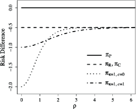
Figure 1: The asymptotic risk difference
N 2 [ E { D ( p ~ ( y β£ ΞΈ ) , p ~ c , ΞΊ ( y β£ x N ) β£ ΞΈ } β E { D ( p ~ ( y β£ ΞΈ ) , p ~ P ( y β£ x N ) β£ ΞΈ } ] + o ( 1 ) = β ( b ~ / b 2 ) { 1 / 2 + c ( Ο / Ο P ) + ( 3 / 2 ) ( 1 β c 2 ) ( Ο / Ο P ) } 2 N^{2}[{\rm E}\{D(\displaystyle\tilde{p}(y\mid\theta),\displaystyle\tilde{p}_{c,\kappa}(y\mid x^{N})\mid\theta\}-{\rm E}\{D(\displaystyle\tilde{p}(y\mid\theta),\displaystyle\tilde{p}_{\mathrm{P}}(y\mid x^{N})\mid\theta\}]+\mathrm{o}(1)=-(\tilde{b}/b^{2})\{1/2+c(\pi/\pi_{\mathrm{P}})+(3/2)(1-c^{2})(\pi/\pi_{\mathrm{P}})\}^{2}
for Bayesian predictive densities based on Ο P subscript π P \pi_{\mathrm{P}} , Ο R subscript π R \pi_{\mathrm{R}} , Ο C subscript π C \pi_{\mathrm{C}} ,
Ο ΞΊ = 1 , c = 0 subscript π formulae-sequence π
1 π 0 \pi_{\kappa=1,c=0} , and Ο ΞΊ = 1 , c = 1 subscript π formulae-sequence π
1 π 1 \pi_{\kappa=1,c=1} .
We put b ~ / b 2 = 1 ~ π superscript π 2 1 \tilde{b}/b^{2}=1 just for simplicity.
Several properties of the function (14 ) are discussed in Komaki (2007 ) .
As ΞΊ β β β π
\kappa\to\infty , the prior Ο c , ΞΊ subscript π π π
\pi_{c,\kappa} converges to the right invariant prior Ο R subscript π R \pi_{\mathrm{R}} ,
because
Ο c , ΞΊ β ( ΞΌ , Ο ) Ο P β ( ΞΌ , Ο ) = 1 a 2 β b ~ b 2 β a ~ β ΞΌ 2 + Ο 2 + ΞΊ 2 2 β Ο β ΞΊ + c β ΞΊ / 2 a 2 β b ~ b 2 β a ~ β ΞΌ 2 + Ο 2 + ΞΊ 2 2 β Ο β ΞΊ + c β Ο subscript π π π
π π subscript π P π π 1 superscript π 2 ~ π superscript π 2 ~ π superscript π 2 superscript π 2 superscript π
2 2 π π
π proportional-to π
2 superscript π 2 ~ π superscript π 2 ~ π superscript π 2 superscript π 2 superscript π
2 2 π π
π β π \displaystyle\frac{\pi_{c,\kappa}(\mu,\sigma)}{\pi_{\mathrm{P}}(\mu,\sigma)}=\frac{1}{\displaystyle\frac{\frac{a^{2}\tilde{b}}{b^{2}\tilde{a}}\mu^{2}+\sigma^{2}+\kappa^{2}}{2\sigma\kappa}+c}\propto\frac{\kappa/2}{\displaystyle\frac{\frac{a^{2}\tilde{b}}{b^{2}\tilde{a}}\mu^{2}+\sigma^{2}+\kappa^{2}}{2\sigma\kappa}+c}\rightarrow\sigma
when ΞΊ β β β π
\kappa\to\infty .
Here, priors are identified up to a positive multiplicative constant.
As ΞΊ β 0 β π
0 \kappa\to 0 , the prior Ο c , ΞΊ subscript π π π
\pi_{c,\kappa} converges to
Ο C β ( ΞΌ , Ο ) β d β ΞΌ β d β Ο subscript π C π π d π d π \displaystyle\pi_{\mathrm{C}}(\mu,\sigma)\mbox{d}\mu\mbox{d}\sigma
:= Ο a 2 β b ~ b 2 β a ~ β ΞΌ 2 + Ο 2 β 1 Ο 2 β d β ΞΌ β d β Ο = Ο β 1 a 2 β b ~ b 2 β a ~ β ( ΞΌ Ο ) 2 + 1 β 1 Ο 2 β d β ΞΌ β d β Ο , assign absent π superscript π 2 ~ π superscript π 2 ~ π superscript π 2 superscript π 2 1 superscript π 2 d π d π superscript π 1 superscript π 2 ~ π superscript π 2 ~ π superscript π π 2 1 1 superscript π 2 d π d π \displaystyle:=\frac{\sigma}{\frac{a^{2}\tilde{b}}{b^{2}\tilde{a}}\mu^{2}+\sigma^{2}}\frac{1}{\sigma^{2}}\mbox{d}\mu\mbox{d}\sigma=\frac{\sigma^{-1}}{\frac{a^{2}\tilde{b}}{b^{2}\tilde{a}}(\frac{\mu}{\sigma})^{2}+1}\frac{1}{\sigma^{2}}\mbox{d}\mu\mbox{d}\sigma,
because
Ο c , ΞΊ β ( ΞΌ , Ο ) Ο P β ( ΞΌ , Ο ) = 1 a 2 β b ~ b 2 β a ~ β ΞΌ 2 + Ο 2 + ΞΊ 2 2 β Ο β ΞΊ + c β 1 / ( 2 β ΞΊ ) a 2 β b ~ b 2 β a ~ β ΞΌ 2 + Ο 2 + ΞΊ 2 2 β Ο β ΞΊ + c β Ο a 2 β b ~ b 2 β a ~ β ΞΌ 2 + Ο 2 subscript π π π
π π subscript π P π π 1 superscript π 2 ~ π superscript π 2 ~ π superscript π 2 superscript π 2 superscript π
2 2 π π
π proportional-to 1 2 π
superscript π 2 ~ π superscript π 2 ~ π superscript π 2 superscript π 2 superscript π
2 2 π π
π β π superscript π 2 ~ π superscript π 2 ~ π superscript π 2 superscript π 2 \displaystyle\frac{\pi_{c,\kappa}(\mu,\sigma)}{\pi_{\mathrm{P}}(\mu,\sigma)}=\frac{1}{\displaystyle\frac{\frac{a^{2}\tilde{b}}{b^{2}\tilde{a}}\mu^{2}+\sigma^{2}+\kappa^{2}}{2\sigma\kappa}+c}\propto\frac{1/(2\kappa)}{\displaystyle\frac{\frac{a^{2}\tilde{b}}{b^{2}\tilde{a}}\mu^{2}+\sigma^{2}+\kappa^{2}}{2\sigma\kappa}+c}\rightarrow\frac{\sigma}{\frac{a^{2}\tilde{b}}{b^{2}\tilde{a}}\mu^{2}+\sigma^{2}}
when ΞΊ β 0 β π
0 \kappa\to 0 .
The prior density with respect to the rescaled parameter ( u , v ) π’ π£ (u,v) defined by (11 ) is given by
Ο C β ( ΞΌ , Ο ) β d β ΞΌ β d β Ο β v β 1 ( u / v ) 2 + 1 β 1 v 2 β d β u β d β v . proportional-to subscript π C π π d π d π superscript π£ 1 superscript π’ π£ 2 1 1 superscript π£ 2 d π’ d π£ \displaystyle\pi_{\mathrm{C}}(\mu,\sigma)\mbox{d}\mu\mbox{d}\sigma\propto\frac{v^{-1}}{(u/v)^{2}+1}\frac{1}{v^{2}}\mbox{d}u\mbox{d}v.
(20)
Note that the Cauchy prior for u π’ u , discussed by Jeffreys and many researchers, appears in (20 ).
Thus, the class Ο c , ΞΊ subscript π π π
\pi_{c,\kappa}
of priors bridges the right invariant prior Ο R subscript π R \pi_{\mathrm{R}} ,
coinciding with the reference prior, and the Cauchy prior Ο C subscript π C \pi_{\mathrm{C}} .
Figure 1 illustrates the difference between the risk functions of Bayesian predictive densities based on
Ο R subscript π R \pi_{\mathrm{R}} , Ο C subscript π C \pi_{\mathrm{C}} , Ο ΞΊ = 1 , c = 0 subscript π formulae-sequence π
1 π 0 \pi_{\kappa=1,c=0} , and Ο ΞΊ = 1 , c = 1 subscript π formulae-sequence π
1 π 1 \pi_{\kappa=1,c=1}
and the risk function of p ~ P β ( y β£ x N ) subscript ~ π P conditional π¦ superscript π₯ π \displaystyle\tilde{p}_{\mathrm{P}}(y\mid x^{N}) .
The risk functions of the right invariant prior Ο R subscript π R \pi_{\mathrm{R}} and the Cauchy prior Ο C subscript π C \pi_{\mathrm{C}}
are uniformly smaller than that of Ο P subscript π P \pi_{\mathrm{P}} .
The asymptotic risk of the Cauchy prior Ο C subscript π C \pi_{\mathrm{C}} coincides with that of Ο R subscript π R \pi_{\mathrm{R}} .
Furthermore, the asymptotic risks of Ο ΞΊ = 1 , c = 0 subscript π formulae-sequence π
1 π 0 \pi_{\kappa=1,c=0} and Ο ΞΊ = 1 , c = 1 subscript π formulae-sequence π
1 π 1 \pi_{\kappa=1,c=1} are smaller than that of
Ο R subscript π R \pi_{\mathrm{R}} for every ( ΞΌ , Ο ) π π (\mu,\sigma) .
Therefore, the use of Ο ΞΊ = 1 , c subscript π π
1 π
\pi_{\kappa=1,c} ( 0 β€ c β€ 1 ) 0 π 1 (0\leq c\leq 1) is recommended.
The risk of Ο ΞΊ = 1 , c = 0 subscript π formulae-sequence π
1 π 0 \pi_{\kappa=1,c=0} is smaller than that of Ο ΞΊ = 1 , c = 1 subscript π formulae-sequence π
1 π 1 \pi_{\kappa=1,c=1} when Ο π \rho is small,
and vice versa.
Thus, there does not exist a unique best value of c π c .
The choice of the value of 0 < ΞΊ < β 0 π
0<\kappa<\infty is arbitrary because it corresponds to the center of shrinkage.
Finite-sample decision theoretic properties such as admissibility of Bayesian predictive densities
p ~ ΞΊ , c β ( y β£ x N ) subscript ~ π π
π
conditional π¦ superscript π₯ π \displaystyle\tilde{p}_{\kappa,c}(y\mid x^{N})
based on proposed priors Ο ΞΊ , c subscript π π
π
\pi_{\kappa,c} ( 0 < ΞΊ < β , 0 β€ c β€ 1 ) formulae-sequence 0 π
0 π 1 (0<\kappa<\infty,~{}0\leq c\leq 1) require further research.
Example 3. Poisson models
Suppose that x i subscript π₯ π x_{i} ( i = 1 , β¦ , d ) π 1 β¦ π
(i=1,\ldots,d) are independently distributed
according to the Poisson distribution Po β ( Ξ» i ) Po subscript π π \mbox{Po}(\lambda_{i}) with mean Ξ» i subscript π π \lambda_{i}
and that y i subscript π¦ π y_{i} ( i = 1 , β¦ , d ) π 1 β¦ π
(i=1,\ldots,d) are independently distributed
according to the Poisson distribution Po β ( s i β Ξ» i ) Po subscript π π subscript π π \mbox{Po}(s_{i}\lambda_{i}) with mean s i β Ξ» i subscript π π subscript π π s_{i}\lambda_{i} .
Here, s i subscript π π s_{i} are known positive constants.
The unknown parameter is ΞΈ = ( ΞΈ 1 , β¦ , ΞΈ d ) := ( Ξ» 1 , β¦ , Ξ» d ) π superscript π 1 β¦ superscript π π assign subscript π 1 β¦ subscript π π \theta=(\theta^{1},\ldots,\theta^{d}):=(\lambda_{1},\ldots,\lambda_{d}) .
The objective is to construct a predictive density for y π¦ y by using x π₯ x .
This problem in the conventional setting, in which s 1 = s 2 = β― = s d subscript π 1 subscript π 2 β― subscript π π s_{1}=s_{2}=\cdots=s_{d} ,
is studied in Komaki (2004 ) .
If s i βͺ 1 much-less-than subscript π π 1 s_{i}\ll 1 for each i π i , then this prediction problem is in the asymptotic setting.
The FisherβRao metrics corresponding to x π₯ x and y π¦ y are given by
g i β j = { 1 Ξ» i ( i = j ) 0 ( i β j ) β and g ~ i β j = { s i Ξ» i ( i = j ) 0 ( i β j ) , formulae-sequence subscript π π π cases 1 subscript π π π π 0 π π and subscript ~ π π π cases subscript π π subscript π π π π 0 π π g_{ij}=\left\{\begin{array}[]{cc}\displaystyle\frac{1}{\lambda_{i}}&(i=j)\\[8.5359pt]
0&(i\neq j)\end{array}\right.~{}~{}~{}\mbox{and}~{}~{}~{}~{}~{}\tilde{g}_{ij}=\left\{\begin{array}[]{cc}\displaystyle\frac{s_{i}}{\lambda_{i}}&(i=j)\\[8.5359pt]
0&(i\neq j)\end{array}\right.,
respectively.
The predictive metric is
g Μ i β j = { 1 s i β Ξ» i ( i = j ) 0 ( i β j ) , subscript Μ π π π cases 1 subscript π π subscript π π π π 0 π π \displaystyle\mathring{g}_{ij}=\left\{\begin{array}[]{cc}\displaystyle\frac{1}{s_{i}\lambda_{i}}&(i=j)\\[8.5359pt]
0&(i\neq j)\end{array}\right.,
(23)
and the corresponding volume element is
Ο P β ( Ξ» ) β d β Ξ» := | g Μ | 1 / 2 β d β Ξ» = { β i = 1 d 1 ( s j β Ξ» j ) 1 / 2 } β d β Ξ» β 1 ( Ξ» 1 β β― β Ξ» d ) 1 / 2 β d β Ξ» assign subscript π P π d π superscript Μ π 1 2 d π superscript subscript product π 1 π 1 superscript subscript π π subscript π π 1 2 d π proportional-to 1 superscript subscript π 1 β― subscript π π 1 2 d π \pi_{\mathrm{P}}(\lambda)\mbox{d}\lambda:=|\mathring{g}|^{1/2}\mbox{d}\lambda=\left\{\prod_{i=1}^{d}\frac{1}{(s_{j}\lambda_{j})^{1/2}}\right\}\mbox{d}\lambda\propto\frac{1}{(\lambda_{1}\cdots\lambda_{d})^{1/2}}\mbox{d}\lambda
coinciding with the Jeffreys priors for p β ( x β£ Ξ» ) π conditional π₯ π p(x\mid\lambda) and p ~ β ( y β£ Ξ» ) ~ π conditional π¦ π \displaystyle\tilde{p}(y\mid\lambda) .
The Laplacian Ξ Μ Μ Ξ \mathring{\Delta}{}{} based on the predictive metric g Μ Μ π \mathring{g} is given by
Ξ Μ β f = ( β k = 1 d Ξ» k 1 / 2 ) β β i = 1 d β β Ξ» i β ( s i β Ξ» i β j = 1 d Ξ» j 1 / 2 β β f β Ξ» i ) = β i s i β ( Ξ» i β β 2 f β Ξ» i 2 + 1 2 β β f β Ξ» i ) , Μ Ξ π superscript subscript product π 1 π superscript subscript π π 1 2 superscript subscript π 1 π subscript π π subscript π π subscript π π superscript subscript product π 1 π superscript subscript π π 1 2 π subscript π π subscript π subscript π π subscript π π superscript 2 π superscript subscript π π 2 1 2 π subscript π π \mathring{\Delta}f=\left(\prod_{k=1}^{d}\lambda_{k}^{1/2}\right)\sum_{i=1}^{d}\frac{\partial}{\partial\lambda_{i}}\left(\frac{s_{i}\lambda_{i}}{\prod_{j=1}^{d}\lambda_{j}^{1/2}}\frac{\partial f}{\partial\lambda_{i}}\right)=\sum_{i}s_{i}\left(\lambda_{i}\frac{\partial^{2}f}{\partial\lambda_{i}^{2}}+\frac{1}{2}\frac{\partial f}{\partial\lambda_{i}}\right),
where f π f is a smooth real function of Ξ» π \lambda .
Define
Ο S β ( Ξ» ) β d β Ξ» := ( Ξ» 1 / s 1 + β― + Ξ» d / s d ) β ( d / 2 β 1 ) β j Ξ» j 1 / 2 β d β Ξ» β ( Ξ» 1 / s 1 + β― + Ξ» d / s d ) β ( d / 2 β 1 ) β | g Μ | 1 / 2 β d β Ξ» . assign subscript π S π d π superscript subscript π 1 subscript π 1 β― subscript π π subscript π π π 2 1 subscript product π superscript subscript π π 1 2 d π proportional-to superscript subscript π 1 subscript π 1 β― subscript π π subscript π π π 2 1 superscript Μ π 1 2 d π \pi_{\mathrm{S}}(\lambda)\mbox{d}\lambda:=\frac{(\lambda_{1}/s_{1}+\cdots+\lambda_{d}/s_{d})^{-(d/2-1)}}{\prod_{j}{\lambda_{j}}^{1/2}}\mbox{d}\lambda\propto(\lambda_{1}/s_{1}+\cdots+\lambda_{d}/s_{d})^{-(d/2-1)}|\mathring{g}|^{1/2}\mbox{d}\lambda.
Then, from
β β Ξ» i β Ο S β ( Ξ» ) Ο P β ( Ξ» ) = ( β d 2 + 1 ) β ( Ξ» 1 s 1 + β― + Ξ» d s d ) β d 2 β 1 s i subscript π π subscript π S π subscript π P π π 2 1 superscript subscript π 1 subscript π 1 β― subscript π π subscript π π π 2 1 subscript π π \displaystyle\frac{\partial}{\partial\lambda_{i}}\frac{\pi_{\mathrm{S}}(\lambda)}{\pi_{\mathrm{P}}(\lambda)}=\left(-\frac{d}{2}+1\right)\left(\frac{\lambda_{1}}{s_{1}}+\dotsb+\frac{\lambda_{d}}{s_{d}}\right)^{-\frac{d}{2}}\frac{1}{s_{i}}
(24)
and
β 2 β Ξ» i 2 β Ο S β ( Ξ» ) Ο P β ( Ξ» ) = ( β d 2 + 1 ) β ( β d 2 ) β ( Ξ» 1 s 1 + β― + Ξ» d s d ) β d 2 β 1 β ( 1 s i ) 2 , superscript 2 subscript superscript π 2 π subscript π S π subscript π P π π 2 1 π 2 superscript subscript π 1 subscript π 1 β― subscript π π subscript π π π 2 1 superscript 1 subscript π π 2 \frac{\partial^{2}}{\partial\lambda^{2}_{i}}\frac{\pi_{\mathrm{S}}(\lambda)}{\pi_{\mathrm{P}}(\lambda)}=\left(-\frac{d}{2}+1\right)\left(-\frac{d}{2}\right)\left(\frac{\lambda_{1}}{s_{1}}+\dotsb+\frac{\lambda_{d}}{s_{d}}\right)^{-\frac{d}{2}-1}\left(\frac{1}{s_{i}}\right)^{2},
we have
Ξ Μ β Ο S β ( Ξ» ) Ο P β ( Ξ» ) = β i s i β ( Ξ» i β β 2 β Ξ» i 2 β Ο S β ( Ξ» ) Ο P β ( Ξ» ) + 1 2 β β β Ξ» i β Ο S β ( Ξ» ) Ο P β ( Ξ» ) ) = 0 . Μ Ξ subscript π S π subscript π P π subscript π subscript π π subscript π π superscript 2 superscript subscript π π 2 subscript π S π subscript π P π 1 2 subscript π π subscript π S π subscript π P π 0 \displaystyle\mathring{\Delta}{}{}\frac{\pi_{\mathrm{S}}(\lambda)}{\pi_{\mathrm{P}}(\lambda)}=\sum_{i}s_{i}\left(\lambda_{i}\frac{\partial^{2}}{\partial\lambda_{i}^{2}}\frac{\pi_{\mathrm{S}}(\lambda)}{\pi_{\mathrm{P}}(\lambda)}+\frac{1}{2}\frac{\partial}{\partial\lambda_{i}}\frac{\pi_{\mathrm{S}}(\lambda)}{\pi_{\mathrm{P}}(\lambda)}\right)=0.
(25)
Since Ο S / Ο P subscript π S subscript π P \pi_{\mathrm{S}}/\pi_{\mathrm{P}} is a non-constant positive superharmonic function of Ξ» π \lambda ,
the Bayesian predictive density p ~ S β ( y β£ x ) subscript ~ π S conditional π¦ π₯ \displaystyle\tilde{p}_{\mathrm{S}}(y\mid x) based on Ο S subscript π S \pi_{\mathrm{S}}
asymptotically dominates p ~ P β ( y β£ x ) subscript ~ π P conditional π¦ π₯ \displaystyle\tilde{p}_{\mathrm{P}}(y\mid x)
by CorollaryΒ 1 .
The model manifold endowed with the predictive metric g Μ i β j subscript Μ π π π \mathring{g}_{ij} is isometric to the first orthant
β + n = { ( x 1 , β― , x n ) : x 1 > 0 , x 2 > 0 , β― , x n > 0 } subscript superscript β π conditional-set superscript π₯ 1 β― superscript π₯ π formulae-sequence superscript π₯ 1 0 formulae-sequence superscript π₯ 2 0 β―
superscript π₯ π 0 \mathbb{R}^{n}_{+}=\{(x^{1},\dotsb,x^{n}):x^{1}>0,x^{2}>0,\dotsb,x^{n}>0\}
of the Euclidean space β n superscript β π \mathbb{R}^{n} , as we see below.
Define
ΞΎ i β² = 2 β ΞΈ i β² s i β² β ( i β² = 1 , β¦ , d ) . superscript π superscript π β² 2 superscript π superscript π β² subscript π superscript π β² superscript π β² 1 β¦ π
\xi^{i^{\prime}}=2\sqrt{\frac{\theta^{i^{\prime}}}{s_{i^{\prime}}}}~{}~{}~{}(i^{\prime}=1,\ldots,d).
Then,
β ΞΈ i β ΞΎ i β² superscript π π superscript π superscript π β² \displaystyle\frac{\partial\theta^{i}}{\partial\xi^{i^{\prime}}}
= { ( s i β² β Ξ» i β² ) 1 2 ( i = i β² ) 0 ( i β i β² ) . absent cases superscript subscript π superscript π β² subscript π superscript π β² 1 2 π superscript π β² 0 π superscript π β² \displaystyle=\begin{cases}(s_{i^{\prime}}\lambda_{i^{\prime}})^{\frac{1}{2}}&(i=i^{\prime})\\
0&(i\neq i^{\prime}).\end{cases}
Thus, from (23 ),
the coefficients of the metric with respect to ( ΞΎ i β² ) superscript π superscript π β² (\xi^{i^{\prime}}) are given by
g Μ i β² β j β² subscript Μ π superscript π β² superscript π β² \displaystyle\mathring{g}_{i^{\prime}j^{\prime}}
= β i , j β ΞΈ i β ΞΎ i β² β g Μ i β j β β ΞΈ j β ΞΎ j β² = { 1 ( i β² = j β² ) 0 ( i β² β j β² ) . absent subscript π π
superscript π π superscript π superscript π β² subscript Μ π π π superscript π π superscript π superscript π β² cases 1 superscript π β² superscript π β² 0 superscript π β² superscript π β² \displaystyle=\sum_{i,j}\frac{\partial\theta^{i}}{\partial\xi^{i^{\prime}}}\mathring{g}_{ij}\frac{\partial\theta^{j}}{\partial\xi^{j^{\prime}}}=\begin{cases}1&(i^{\prime}=j^{\prime})\\
0&(i^{\prime}\neq j^{\prime}).\end{cases}
This coincides with the usual metric on β + n subscript superscript β π \mathbb{R}^{n}_{+} .
Here, the function
β ΞΎ β β d + 2 β Ο S β ( Ξ» ) Ο P β ( Ξ» ) = ( Ξ» 1 s 1 + β― + Ξ» d s d ) β d 2 + 1 proportional-to superscript norm π π 2 subscript π S π subscript π P π superscript subscript π 1 subscript π 1 β― subscript π π subscript π π π 2 1 \|\xi\|^{-d+2}\propto\frac{\pi_{\mathrm{S}}(\lambda)}{\pi_{\mathrm{P}}(\lambda)}=\left(\frac{\lambda_{1}}{s_{1}}+\dotsb+\frac{\lambda_{d}}{s_{d}}\right)^{-\frac{d}{2}+1}
of ΞΎ π \xi
is the Green function of the heat equation on β n superscript β π \mathbb{R}^{n}
and plays an essential role in Bayesian methods for model manifolds isometric to the Euclidean space.
For example, the prior density β ΞΌ β β d + 2 superscript norm π π 2 \|\mu\|^{-d+2} for the d π d -dimensional
Normal model N d β ( ΞΌ , I d ) subscript π π π subscript πΌ π N_{d}(\mu,I_{d}) , where ΞΌ π \mu is the d π d -dimensional unknown mean vector
and I d subscript πΌ π I_{d} is the d Γ d π π d\times d identity matrix, is known as the Stein prior.
The Bayesian predictive density based on Ο P subscript π P \pi_{\mathrm{P}} is
p ~ P β ( y β£ x ) = subscript ~ π P conditional π¦ π₯ absent \displaystyle\displaystyle\tilde{p}_{\mathrm{P}}(y\mid\ x)=
β« β i = 1 d { Ξ» i x i x i ! β e β Ξ» i β ( s i β Ξ» i ) y i y i ! β e β s i β Ξ» i } β β j = 1 d Ξ» j β 1 / 2 β d β Ξ» β« β i = 1 d ( Ξ» i x i x i ! β e β Ξ» i ) β β j = 1 d Ξ» j β 1 / 2 β d β Ξ» superscript subscript product π 1 π superscript subscript π π subscript π₯ π subscript π₯ π superscript e subscript π π superscript subscript π π subscript π π subscript π¦ π subscript π¦ π superscript e subscript π π subscript π π superscript subscript product π 1 π superscript subscript π π 1 2 d π superscript subscript product π 1 π superscript subscript π π subscript π₯ π subscript π₯ π superscript e subscript π π superscript subscript product π 1 π superscript subscript π π 1 2 d π \displaystyle\frac{\displaystyle\int\prod_{i=1}^{d}\left\{\frac{{\lambda_{i}}^{x_{i}}}{x_{i}!}\mbox{e}^{-\lambda_{i}}\frac{(s_{i}\lambda_{i})^{y_{i}}}{y_{i}!}\mbox{e}^{-s_{i}\lambda_{i}}\right\}\prod_{j=1}^{d}{\lambda_{j}}^{-1/2}\mbox{d}\lambda}{\displaystyle\int\prod_{i=1}^{d}\left(\frac{{\lambda_{i}}^{x_{i}}}{x_{i}!}\mbox{e}^{-\lambda_{i}}\right)\prod_{j=1}^{d}{\lambda_{j}}^{-1/2}\mbox{d}\lambda}
= \displaystyle=
β i = 1 d { s i y i ( 1 + s i ) x i + y i + 1 / 2 β Ξ β ( x i + y i + 1 / 2 ) x i ! β y i ! } β i = 1 d Ξ β ( x i + 1 / 2 ) x i ! superscript subscript product π 1 π superscript subscript π π subscript π¦ π superscript 1 subscript π π subscript π₯ π subscript π¦ π 1 2 Ξ subscript π₯ π subscript π¦ π 1 2 subscript π₯ π subscript π¦ π superscript subscript product π 1 π Ξ subscript π₯ π 1 2 subscript π₯ π \displaystyle\frac{\displaystyle\prod_{i=1}^{d}\left\{\frac{s_{i}^{y_{i}}}{(1+s_{i})^{x_{i}+y_{i}+1/2}}\frac{\Gamma(x_{i}+y_{i}+1/2)}{x_{i}!y_{i}!}\right\}}{\displaystyle\prod_{i=1}^{d}\frac{\Gamma(x_{i}+1/2)}{x_{i}!}}
= \displaystyle=
β i = 1 d { s i y i ( 1 + s i ) x i + y i + 1 / 2 β Ξ β ( x i + y i + 1 / 2 ) Ξ β ( x i + 1 / 2 ) β y i ! } , superscript subscript product π 1 π superscript subscript π π subscript π¦ π superscript 1 subscript π π subscript π₯ π subscript π¦ π 1 2 Ξ subscript π₯ π subscript π¦ π 1 2 Ξ subscript π₯ π 1 2 subscript π¦ π \displaystyle\displaystyle\prod_{i=1}^{d}\left\{\frac{s_{i}^{y_{i}}}{(1+s_{i})^{x_{i}+y_{i}+1/2}}\frac{\Gamma(x_{i}+y_{i}+1/2)}{\Gamma(x_{i}+1/2)y_{i}!}\right\},
where d β Ξ» := d β Ξ» 1 β β― β d β Ξ» d assign d π d subscript π 1 β― d subscript π π \mbox{d}\lambda:=\mbox{d}\lambda_{1}\cdots\mbox{d}\lambda_{d} .
The Bayesian predictive density based on Ο S subscript π S \pi_{\mathrm{S}} is
p ~ S β ( y β£ x ) subscript ~ π S conditional π¦ π₯ \displaystyle\displaystyle\tilde{p}_{\mathrm{S}}(y\mid x)
= β« β i = 1 d { Ξ» i x i x i ! β e β Ξ» i β ( s i β Ξ» i ) y i y i ! β e β s i β Ξ» i } β ( β j = 1 d Ξ» j s j ) β ( d / 2 β 1 ) β β k = 1 d Ξ» k β 1 / 2 β d β Ξ» β« β i = 1 d ( Ξ» i x i x i ! β e β Ξ» i ) β ( β j = 1 d Ξ» j s j ) β ( d / 2 β 1 ) β β k = 1 d Ξ» k β 1 / 2 β d β Ξ» absent superscript subscript product π 1 π superscript subscript π π subscript π₯ π subscript π₯ π superscript e subscript π π superscript subscript π π subscript π π subscript π¦ π subscript π¦ π superscript e subscript π π subscript π π superscript superscript subscript π 1 π subscript π π subscript π π π 2 1 superscript subscript product π 1 π superscript subscript π π 1 2 d π superscript subscript product π 1 π superscript subscript π π subscript π₯ π subscript π₯ π superscript e subscript π π superscript superscript subscript π 1 π subscript π π subscript π π π 2 1 superscript subscript product π 1 π superscript subscript π π 1 2 d π \displaystyle=\frac{\displaystyle\int\prod_{i=1}^{d}\left\{\frac{{\lambda_{i}}^{x_{i}}}{x_{i}!}\mbox{e}^{-\lambda_{i}}\frac{(s_{i}\lambda_{i})^{y_{i}}}{y_{i}!}\mbox{e}^{-s_{i}\lambda_{i}}\right\}\biggl{(}\sum_{j=1}^{d}\frac{\lambda_{j}}{s_{j}}\biggr{)}^{-(d/2-1)}\prod_{k=1}^{d}{\lambda_{k}}^{-1/2}\mbox{d}\lambda}{\displaystyle\int\prod_{i=1}^{d}\left(\frac{{\lambda_{i}}^{x_{i}}}{x_{i}!}\mbox{e}^{-\lambda_{i}}\right)\biggl{(}\sum_{j=1}^{d}\frac{\lambda_{j}}{s_{j}}\biggr{)}^{-(d/2-1)}\prod_{k=1}^{d}{\lambda_{k}}^{-1/2}\mbox{d}\lambda}
= β« β i = 1 d { s i y i β Ξ» i x i + y i β 1 / 2 y i ! β e β ( 1 + s i ) β Ξ» i } β { β« 0 β u d 2 β 2 β exp β‘ ( β u β β j Ξ» j s j ) β d β u } β d β Ξ» β« β i = 1 d ( Ξ» i x i β 1 / 2 β e β Ξ» i ) β { β« 0 β u d 2 β 2 β exp β‘ ( β u β β j Ξ» j s j ) β d β u } β d β Ξ» absent superscript subscript product π 1 π superscript subscript π π subscript π¦ π superscript subscript π π subscript π₯ π subscript π¦ π 1 2 subscript π¦ π superscript e 1 subscript π π subscript π π superscript subscript 0 superscript π’ π 2 2 π’ subscript π subscript π π subscript π π d π’ d π superscript subscript product π 1 π superscript subscript π π subscript π₯ π 1 2 superscript e subscript π π superscript subscript 0 superscript π’ π 2 2 π’ subscript π subscript π π subscript π π d π’ d π \displaystyle=\frac{\displaystyle\int\prod_{i=1}^{d}\left\{\frac{s_{i}^{y_{i}}\lambda_{i}^{x_{i}+y_{i}-1/2}}{y_{i}!}\mbox{e}^{-(1+s_{i})\lambda_{i}}\right\}\left\{\int_{0}^{\infty}u^{\frac{d}{2}-2}\exp\Bigl{(}-u\sum_{j}\frac{\lambda_{j}}{s_{j}}\Bigr{)}\mbox{d}u\right\}\mbox{d}\lambda}{\displaystyle\int\prod_{i=1}^{d}\left({\lambda_{i}}^{x_{i}-1/2}\mbox{e}^{-\lambda_{i}}\right)\left\{\int_{0}^{\infty}u^{\frac{d}{2}-2}\exp\Bigl{(}-u\sum_{j}\frac{\lambda_{j}}{s_{j}}\Bigr{)}\mbox{d}u\right\}\mbox{d}\lambda}
= β« 0 β u d 2 β 2 β β i = 1 d ( 1 + s i + u / s i ) β ( x i + y i + 1 / 2 ) β d β u β« 0 β u d 2 β 2 β β i = 1 d ( 1 + u / s i ) β ( x i + 1 / 2 ) β d β u β β i = 1 d s i y i β Ξ β ( x i + y i + 1 / 2 ) y i ! β Ξ β ( x i + 1 / 2 ) . absent superscript subscript 0 superscript π’ π 2 2 superscript subscript product π 1 π superscript 1 subscript π π π’ subscript π π subscript π₯ π subscript π¦ π 1 2 d π’ superscript subscript 0 superscript π’ π 2 2 superscript subscript product π 1 π superscript 1 π’ subscript π π subscript π₯ π 1 2 d π’ superscript subscript product π 1 π superscript subscript π π subscript π¦ π Ξ subscript π₯ π subscript π¦ π 1 2 subscript π¦ π Ξ subscript π₯ π 1 2 \displaystyle=\frac{\displaystyle\int_{0}^{\infty}u^{\frac{d}{2}-2}\prod_{i=1}^{d}(1+s_{i}+u/s_{i})^{-(x_{i}+y_{i}+1/2)}\mbox{d}u}{\displaystyle\int_{0}^{\infty}u^{\frac{d}{2}-2}\prod_{i=1}^{d}(1+u/s_{i})^{-(x_{i}+1/2)}\mbox{d}u}\prod_{i=1}^{d}\frac{s_{i}^{y_{i}}\Gamma(x_{i}+y_{i}+1/2)}{y_{i}!\Gamma(x_{i}+1/2)}.
We have the asymptotic risk difference
N 2 [ E { \displaystyle N^{2}\biggl{[}{\rm E}\big{\{}
D ( p ~ ( y β£ ΞΈ ) , p ~ S ( y β£ x ) | ΞΈ } β E { D ( p ~ ( y β£ ΞΈ ) , p ~ P ( y β£ x ) | ΞΈ } ] \displaystyle D(\displaystyle\tilde{p}(y\mid\theta),\displaystyle\tilde{p}_{\mathrm{S}}(y\mid x)\,\big{|}\,\theta\big{\}}-{\rm E}\big{\{}D(\displaystyle\tilde{p}(y\mid\theta),\displaystyle\tilde{p}_{\mathrm{P}}(y\mid x)\,\big{|}\,\theta\big{\}}\biggr{]}
= \displaystyle=
Ξ Μ β ( Ο S / Ο P ) Ο S / Ο P β 1 2 β β i , j g Μ i β j β β i ( Ο S / Ο P ) β β j ( Ο S / Ο P ) ( Ο S / Ο P ) 2 + o β ( 1 ) Μ Ξ subscript π S subscript π P subscript π S subscript π P 1 2 subscript π π
superscript Μ π π π subscript π subscript π S subscript π P subscript π subscript π S subscript π P superscript subscript π S subscript π P 2 o 1 \displaystyle\frac{\mathring{\Delta}(\pi_{\mathrm{S}}/\pi_{\mathrm{P}})}{\pi_{\mathrm{S}}/\pi_{\mathrm{P}}}-\frac{1}{2}\sum_{i,j}\mathring{g}^{ij}\frac{\partial_{i}(\pi_{\mathrm{S}}/\pi_{\mathrm{P}})\partial_{j}(\pi_{\mathrm{S}}/\pi_{\mathrm{P}})}{(\pi_{\mathrm{S}}/\pi_{\mathrm{P}})^{2}}+\mathrm{o}(1)
= \displaystyle=
β 1 2 β ( d 2 β 1 ) 2 β ( Ξ» 1 s 1 + β― + Ξ» d s d ) β 1 + o β ( 1 ) 1 2 superscript π 2 1 2 superscript subscript π 1 subscript π 1 β― subscript π π subscript π π 1 o 1 \displaystyle-\frac{1}{2}\left(\frac{d}{2}-1\right)^{2}\left(\frac{\lambda_{1}}{s_{1}}+\dotsb+\frac{\lambda_{d}}{s_{d}}\right)^{-1}+\mathrm{o}(1)
(26)
by Theorem 2 , (24 ), (25 ), and
g Μ i β j = { s i β Ξ» i ( i = j ) 0 ( i β j ) . superscript Μ π π π cases subscript π π subscript π π π π 0 π π \mathring{g}^{ij}=\begin{cases}s_{i}\lambda_{i}&(i=j)\\
0&(i\neq j).\end{cases}
The asymptotic risk difference (26 ) depends on Ξ» π \lambda only through Ξ» 1 / s 1 + β― + Ξ» d / s d subscript π 1 subscript π 1 β― subscript π π subscript π π \lambda_{1}/s_{1}+\dotsb+\lambda_{d}/s_{d} .
When Ξ» 1 / s 1 + β― + Ξ» d / s d subscript π 1 subscript π 1 β― subscript π π subscript π π \lambda_{1}/s_{1}+\dotsb+\lambda_{d}/s_{d} is small the improvement is large,
and it converges to zero as Ξ» 1 / s 1 + β― + Ξ» d / s d subscript π 1 subscript π 1 β― subscript π π subscript π π \lambda_{1}/s_{1}+\dotsb+\lambda_{d}/s_{d} goes to infinity.
It can be shown that Ο S subscript π S \pi_{\mathrm{S}} dominates Ο P subscript π P \pi_{\mathrm{P}} in the sense of
infinitesimal prediction, and
we can construct
a Bayesian predictive density
dominating p ~ P β ( y β£ x ) subscript ~ π P conditional π¦ π₯ \tilde{p}_{\mathrm{P}}(y\mid x)
for arbitrary s i > 0 subscript π π 0 s_{i}>0 ( i = 1 , β¦ , d ) π 1 β¦ π
(i=1,\ldots,d)
by modifying the prior Ο S subscript π S \pi_{\mathrm{S}} .
Finite sample properties of this prior will be discussed in a another paper
by using an approach different from the asymptotic methods in the present paper.
In Examples 1, 2, and 3,
the volume element based on the predictive metric g Μ i β j subscript Μ π π π \mathring{g}_{ij}
coincides with the Jeffreys priors based on g i β j subscript π π π g_{ij} and g ~ i β j subscript ~ π π π \tilde{g}_{ij} ,
i.e.
| g Μ i β j β ( ΞΈ ) | 1 / 2 β | g i β j β ( ΞΈ ) | 1 / 2 β | g ~ i β j β ( ΞΈ ) | 1 / 2 proportional-to superscript subscript Μ π π π π 1 2 superscript subscript π π π π 1 2 proportional-to superscript subscript ~ π π π π 1 2 |\mathring{g}_{ij}(\theta)|^{1/2}\propto|g_{ij}(\theta)|^{1/2}\propto|\tilde{g}_{ij}(\theta)|^{1/2} ,
although the three metrics are different.
In general, if two metrics g i β j subscript π π π g_{ij} and g ~ i β j subscript ~ π π π \tilde{g}_{ij} satisfy the relation
g ~ i β j β ( ΞΈ ) = β k , l g k β l β ( ΞΈ ) β A i k β A j l , subscript ~ π π π π subscript π π
subscript π π π π subscript superscript π΄ π π subscript superscript π΄ π π \displaystyle\tilde{g}_{ij}(\theta)=\sum_{k,l}g_{kl}(\theta)A^{k}_{i}A^{l}_{j},
(27)
where ( A j i ) subscript superscript π΄ π π (A^{i}_{j}) is a d Γ d π π d\times d regular matrix not depending on ΞΈ π \theta ,
then
| g ~ i β j | 1 2 = | A k l | β | g i β j | 1 2 , and β | g Μ i β j | 1 2 = | g i β j | β | g ~ i β j | β 1 2 = | A k l | β 1 β | g i β j | 1 2 formulae-sequence superscript subscript ~ π π π 1 2 subscript superscript π΄ π π superscript subscript π π π 1 2 and superscript subscript Μ π π π 1 2 subscript π π π superscript subscript ~ π π π 1 2 superscript subscript superscript π΄ π π 1 superscript subscript π π π 1 2 |\tilde{g}_{ij}|^{\frac{1}{2}}=|A^{l}_{k}||g_{ij}|^{\frac{1}{2}},~{}~{}\mbox{and}~{}~{}|\mathring{g}_{ij}|^{\frac{1}{2}}=|g_{ij}||\tilde{g}_{ij}|^{-\frac{1}{2}}=|A^{l}_{k}|^{-1}|g_{ij}|^{\frac{1}{2}}
and the volume elements based on g i β j subscript π π π g_{ij} , g ~ i β j subscript ~ π π π \tilde{g}_{ij} , and g Μ i β j subscript Μ π π π \mathring{g}_{ij} are proportional to each other.
The relation (27 ) appears in many examples as in Examples 1, 2, and 3.
Appendix. Proofs of Theorems 1 and 2
First, we prepare a preliminary result, Theorem 1 , to prove Theorem 1 .
Asymptotic properties of predictive densities in the conventional setting in which x β ( i ) π₯ π x(i) , i = 1 , β¦ , N π 1 β¦ π
i=1,\ldots,N , and y π¦ y have
the same distribution have been studied, see Komaki (1996 ) , Hartigan (1998 ) , and Sweeting etΒ al. (2006 ) .
Fushiki etΒ al. (2004 ) generalized these results for the setting in which x β ( i ) π₯ π x(i) , i = 1 , β¦ , N π 1 β¦ π
i=1,\ldots,N , and y π¦ y
have different distributions.
The Bayesian predictive density is expanded as
p ~ Ο subscript ~ π π \displaystyle\displaystyle\tilde{p}_{\pi}
( y β£ x N ) = p ~ β ( y β£ ΞΈ ^ mle ) + 1 2 β N β β i , j g i β j β ( ΞΈ ^ mle ) β { β i β j p ~ β ( y β£ ΞΈ ^ mle ) β β k Ξ ~ i β j ( m ) β k β β k p ~ β ( y β£ ΞΈ ^ mle ) } conditional π¦ superscript π₯ π ~ π conditional π¦ subscript ^ π mle 1 2 π subscript π π
superscript π π π subscript ^ π mle subscript π subscript π ~ π conditional π¦ subscript ^ π mle subscript π superscript subscript ~ Ξ π π m π subscript π ~ π conditional π¦ subscript ^ π mle \displaystyle(y\mid x^{N})=\displaystyle\tilde{p}(y\mid\hat{\theta}_{\mathrm{mle}})+\frac{1}{2N}\sum_{i,j}g^{ij}(\hat{\theta}_{\mathrm{mle}})\left\{\partial_{i}\partial_{j}\displaystyle\tilde{p}(y\mid\hat{\theta}_{\mathrm{mle}})-\sum_{k}\tilde{\Gamma}_{ij}^{\,(\mathrm{m})k}\partial_{k}\displaystyle\tilde{p}(y\mid\hat{\theta}_{\mathrm{mle}})\right\}
+ 1 2 β N β k [ β i , j g i β j ( ΞΈ ^ mle ) { Ξ ~ i β j ( m ) β k ( ΞΈ ^ mle ) β Ξ i β j ( m ) β k ( ΞΈ ^ mle ) } \displaystyle+\frac{1}{2N}\sum_{k}\left[\sum_{i,j}g^{ij}(\hat{\theta}_{\mathrm{mle}})\left\{\tilde{\Gamma}_{ij}^{\,(\mathrm{m})k}(\hat{\theta}_{\mathrm{mle}})-\raise 1.5pt\hbox{$\displaystyle\mathop{\Gamma}$}_{ij}^{\,(\mathrm{m})k}(\hat{\theta}_{\mathrm{mle}})\right\}\right.
+ 2 β i g i β k ( ΞΈ ^ mle ) { β i log Ο ( ΞΈ ^ mle ) β β j Ξ i β j ( e ) β j ( ΞΈ ^ mle ) } ] β k p ~ ( y β£ ΞΈ ^ mle ) + o p ( N β 1 ) , \displaystyle~{}~{}~{}~{}~{}~{}\left.+2\sum_{i}g^{ik}(\hat{\theta}_{\mathrm{mle}})\left\{\partial_{i}\log\pi(\hat{\theta}_{\mathrm{mle}})-\sum_{j}\Gamma_{ij}^{(\mathrm{e})j}(\hat{\theta}_{\mathrm{mle}})\right\}\right]\partial_{k}\displaystyle\tilde{p}(y\mid\hat{\theta}_{\mathrm{mle}})+\mathrm{o}_{\mathrm{p}}(N^{-1}),
(28)
where ΞΈ ^ mle subscript ^ π mle \hat{\theta}_{\mathrm{mle}} is the maximum likelihood estimator, and β i := β / β ΞΈ i assign subscript π superscript π π \partial_{i}:=\partial/\partial\theta^{i} .
The estimatorminimizing the Bayes risk
β« E β [ D β { p ~ β ( y β£ ΞΈ ) , p ~ Ο β ( y β£ x ) } | ΞΈ ] β Ο β ( ΞΈ ) β d β ΞΈ E delimited-[] conditional π· ~ π conditional π¦ π subscript ~ π π conditional π¦ π₯ π π π d π \int{\rm E}[D\{\displaystyle\tilde{p}(y\mid\theta),\displaystyle\tilde{p}_{\pi}(y\mid x)\}|\theta]\pi(\theta)\mbox{d}\theta
is given by
ΞΈ ^ Ο i = ΞΈ ^ ππ
πΎ i + 1 N β w Ο i β ( ΞΈ ^ ππ
πΎ ) + o p β ( N β 1 ) , subscript superscript ^ π π π subscript superscript ^ π π ππ
πΎ 1 π subscript superscript π€ π π subscript ^ π ππ
πΎ subscript o p superscript π 1 \hat{\theta}^{i}_{\pi}=\hat{\theta}^{i}_{\sf mle}+\frac{1}{N}w^{i}_{\pi}(\hat{\theta}_{\sf mle})+\mathrm{o}_{\mathrm{p}}(N^{-1}),
(29)
where
w Ο i β ( ΞΈ ) := β k g i β k β ( ΞΈ ) β { β k log β‘ Ο β ( ΞΈ ) β β j Ξ k β j ( e ) β j β ( ΞΈ ) } + 1 2 β β k , l g k β l β ( ΞΈ ) β { Ξ ~ k β l ( m ) β i β ( ΞΈ ) β Ξ k β l ( m ) β i ( ΞΈ ) } , assign subscript superscript π€ π π π subscript π superscript π π π π subscript π π π subscript π superscript subscript Ξ π π e π π 1 2 subscript π π
superscript π π π π superscript subscript ~ Ξ π π m π π superscript subscript Ξ π π m π π w^{i}_{\pi}(\theta):=\sum_{k}g^{ik}(\theta)\Bigl{\{}\partial_{k}\log\pi(\theta)-\sum_{j}\Gamma_{kj}^{(\mathrm{e})j}(\theta)\Bigr{\}}+\frac{1}{2}\sum_{k,l}g^{kl}(\theta)\Bigl{\{}\tilde{\Gamma}_{kl}^{\,(\mathrm{m})i}(\theta)-\raise 1.5pt\hbox{$\displaystyle\mathop{\Gamma}$}_{kl}^{\,(\mathrm{m})i}(\theta)\Bigr{\}},
(30)
which is a covariant vector.
The expansion of the risk function of a Bayesian predictive density p ~ Ο β ( y β£ x N ) subscript ~ π π conditional π¦ superscript π₯ π \displaystyle\tilde{p}_{\pi}(y\mid x^{N}) up to the order N β 2 superscript π 2 N^{-2} is given in
Theorem 1 below.
The expansion is invariant in the sense that
each term is a scalar not depending on parametrization.
In Theorem 1 , we put
v i β j ( e ) β ( x ; ΞΈ ) := assign superscript subscript π£ π π e π₯ π
absent \displaystyle v_{ij}^{\mathrm{(e)}}(x;\theta):=
β i β j log β‘ p β ( x β£ ΞΈ ) + g i β j β ( ΞΈ ) β β k Ξ i β j ( e ) β k β ( ΞΈ ) β β k log β‘ p β ( x β£ ΞΈ ) , subscript π subscript π π conditional π₯ π subscript π π π π subscript π superscript subscript Ξ π π e π π subscript π π conditional π₯ π \displaystyle\partial_{i}\partial_{j}\log p(x\mid\theta)+g_{ij}(\theta)-\sum_{k}\Gamma_{ij}^{(\mathrm{e})k}(\theta)\partial_{k}\log p(x\mid\theta),
v ~ i β j ( m ) β ( y ; ΞΈ ) := assign superscript subscript ~ π£ π π m π¦ π
absent \displaystyle\tilde{v}_{ij}^{\mathrm{(m)}}(y;\theta):=
1 p ~ β ( y β£ ΞΈ ) β { β i β j p ~ β ( y β£ ΞΈ ) β β k Ξ ~ i β j ( m ) β k β β k p ~ β ( y β£ ΞΈ ) } , 1 ~ π conditional π¦ π subscript π subscript π ~ π conditional π¦ π subscript π superscript subscript ~ Ξ π π m π subscript π ~ π conditional π¦ π \displaystyle\frac{1}{\displaystyle\tilde{p}(y\mid\theta)}\Bigl{\{}\partial_{i}\partial_{j}\displaystyle\tilde{p}(y\mid\theta)-\sum_{k}\tilde{\Gamma}_{ij}^{\,(\mathrm{m})k}\partial_{k}\displaystyle\tilde{p}(y\mid\theta)\Bigr{\}},
T i β j β k := assign superscript π π π π absent \displaystyle T^{ijk}:=
β l , m , n T l β m β n β g i β l β g j β m β g k β n , Β andΒ β v ( e ) β i β k := β j , l v j β l ( e ) β g i β j β g k β l . assign subscript π π π
subscript π π π π superscript π π π superscript π π π superscript π π π Β andΒ superscript π£ e π π
subscript π π
superscript subscript π£ π π e superscript π π π superscript π π π \displaystyle\sum_{l,m,n}T_{lmn}g^{il}g^{jm}g^{kn},\mbox{~{}~{}and~{}~{}}v^{\mathrm{(e)}ik}:=\sum_{j,l}v_{jl}^{\mathrm{(e)}}g^{ij}g^{kl}.
Here, v i β j ( e ) superscript subscript π£ π π e v_{ij}^{\mathrm{(e)}} and v ~ i β j ( m ) superscript subscript ~ π£ π π m \tilde{v}_{ij}^{\mathrm{(m)}} are vectors orthogonal to the model manifolds
{ p ( x β£ ΞΈ ) | ΞΈ β Ξ ) } \{p(x\mid\theta)\,|\,\theta\in\Theta)\} and { p ~ ( y β£ ΞΈ ) | ΞΈ β Ξ ) } \{\displaystyle\tilde{p}(y\mid\theta)\,|\,\theta\in\Theta)\} , respectively.
These vectors are closely related to the curvature of the manifolds.
Theorem 1 .
The expected KullbackβLeibler divergence from the true density p ~ β ( y β£ ΞΈ ) ~ π conditional π¦ π \displaystyle\tilde{p}(y\mid\theta)
to the Bayesian predictive density p ~ Ο β ( y β£ x N ) subscript ~ π π conditional π¦ superscript π₯ π \displaystyle\tilde{p}_{\pi}(y\mid x^{N}) based on a prior Ο β ( ΞΈ ) π π \pi(\theta) is expanded as
E { \displaystyle{\rm E}\Bigl{\{}
D ( p ~ ( y β£ ΞΈ ) , p ~ Ο ( y β£ x N ) ) | ΞΈ } \displaystyle D\bigl{(}\displaystyle\tilde{p}(y\mid\theta),\displaystyle\tilde{p}_{\pi}(y\mid x^{N})\bigr{)}\,\Big{|}\,\theta\Bigr{\}}
= \displaystyle=
1 2 β N β β i , j g ~ i β j β g i β j + 1 2 β N 2 β β i , j g ~ i β j β u Ο i β u Ο j + 1 N 2 β β i , j , k g ~ i β j β g j β k β β ~ k ( e ) β u Ο i 1 2 π subscript π π
subscript ~ π π π superscript π π π 1 2 superscript π 2 subscript π π
subscript ~ π π π superscript subscript π’ π π superscript subscript π’ π π 1 superscript π 2 subscript π π π
subscript ~ π π π superscript π π π superscript subscript ~ β π e superscript subscript π’ π π \displaystyle\frac{1}{2N}\sum_{i,j}\tilde{g}_{ij}g^{ij}+\frac{1}{2N^{2}}\sum_{i,j}\tilde{g}_{ij}u_{\pi}^{i}u_{\pi}^{j}+\frac{1}{N^{2}}\sum_{i,j,k}\tilde{g}_{ij}g^{jk}\widetilde{\nabla}_{k}^{(\mathrm{e})}u_{\pi}^{i}
+ 1 2 β N 2 β β i , j , k , l E β ( v ( e ) β i β k β v ( e ) β j β l | ΞΈ ) β g k β l β g ~ i β j 1 2 superscript π 2 subscript π π π π
E conditional superscript π£ e π π superscript π£ e π π π subscript π π π subscript ~ π π π \displaystyle+\frac{1}{2N^{2}}\sum_{i,j,k,l}{\rm E}\left(v^{\mathrm{(e)}ik}v^{\mathrm{(e)}jl}\,\Big{|}\,\theta\right)g_{kl}\tilde{g}_{ij}
β 1 2 β N 2 β β i , j , k , l E β ( v ~ i β j ( m ) β v ~ k β l ( m ) | ΞΈ ) β g i β j β g k β l β 1 3 β N 2 β β i , j , k T ~ i β j β k β T i β j β k 1 2 superscript π 2 subscript π π π π
E conditional superscript subscript ~ π£ π π m superscript subscript ~ π£ π π m π superscript π π π superscript π π π 1 3 superscript π 2 subscript π π π
subscript ~ π π π π superscript π π π π \displaystyle-\frac{1}{2N^{2}}\sum_{i,j,k,l}{\rm E}\left(\tilde{v}_{ij}^{\mathrm{(m)}}\tilde{v}_{kl}^{\mathrm{(m)}}\,\Big{|}\,\theta\right)g^{ij}g^{kl}-\frac{1}{3N^{2}}\sum_{i,j,k}\widetilde{T}_{ijk}T^{ijk}
+ 3 4 β N 2 β β i , j , k , l Q ~ i β j β k β l β g i β j β g k β l β 1 N 2 β β i , j , k , l E β ( β i l ~ β β j l ~ β v ~ k β l ( m ) | ΞΈ ) β g i β k β g j β l 3 4 superscript π 2 subscript π π π π
subscript ~ π π π π π superscript π π π superscript π π π 1 superscript π 2 subscript π π π π
E conditional subscript π ~ π subscript π ~ π superscript subscript ~ π£ π π m π superscript π π π superscript π π π \displaystyle+\frac{3}{4N^{2}}\sum_{i,j,k,l}\tilde{Q}_{ijkl}g^{ij}g^{kl}-\frac{1}{N^{2}}\sum_{i,j,k,l}{\rm E}\left(\partial_{i}\displaystyle\tilde{l}\partial_{j}\displaystyle\tilde{l}\,\tilde{v}_{kl}^{\mathrm{(m)}}\,\Big{|}\,\theta\right)g^{ik}g^{jl}
+ 1 4 β N 2 β β i , j , k , l E β ( v ~ i β j ( m ) β v ~ k β l ( m ) | ΞΈ ) β g i β k β g j β l 1 4 superscript π 2 subscript π π π π
E conditional superscript subscript ~ π£ π π m superscript subscript ~ π£ π π m π superscript π π π superscript π π π \displaystyle+\frac{1}{4N^{2}}\sum_{i,j,k,l}{\rm E}\left(\tilde{v}_{ij}^{\mathrm{(m)}}\tilde{v}_{kl}^{\mathrm{(m)}}\,\Big{|}\,\theta\right)g^{ik}g^{jl}
+ 1 4 β N 2 β β i , j , k , l , m , n g ~ i β j β ( Ξ ~ k β l ( m ) β i β Ξ k β l ( m ) β i ) β ( Ξ ~ m β n ( m ) β j β Ξ m β n ( m ) β j ) β g k β m β g l β n 1 4 superscript π 2 subscript π π π π π π
subscript ~ π π π superscript subscript ~ Ξ π π m π superscript subscript Ξ π π m π superscript subscript ~ Ξ π π m π superscript subscript Ξ π π m π superscript π π π superscript π π π \displaystyle+\frac{1}{4N^{2}}\sum_{i,j,k,l,m,n}\tilde{g}_{ij}(\tilde{\Gamma}_{kl}^{\,(\mathrm{m})i}-\raise 1.5pt\hbox{$\displaystyle\mathop{\Gamma}$}_{kl}^{\,(\mathrm{m})i})(\tilde{\Gamma}_{mn}^{\,(\mathrm{m})j}-\raise 1.5pt\hbox{$\displaystyle\mathop{\Gamma}$}_{mn}^{\,(\mathrm{m})j})g^{km}g^{ln}
β 1 N 2 β β i , j , k , l , m T ~ i β j β k β ( Ξ ~ l β m ( m ) β k β Ξ l β m ( m ) β k ) β g i β l β g j β m + o β ( N β 2 ) , 1 superscript π 2 subscript π π π π π
subscript ~ π π π π superscript subscript ~ Ξ π π m π superscript subscript Ξ π π m π superscript π π π superscript π π π o superscript π 2 \displaystyle-\frac{1}{N^{2}}\sum_{i,j,k,l,m}\widetilde{T}_{ijk}(\tilde{\Gamma}_{lm}^{\,(\mathrm{m})k}-\raise 1.5pt\hbox{$\displaystyle\mathop{\Gamma}$}_{lm}^{\,(\mathrm{m})k})g^{il}g^{jm}+\mathrm{o}(N^{-2}),
(31)
where
u Ο i β ( ΞΈ ) := β k g i β k β ( ΞΈ ) β { β k log β‘ Ο β ( ΞΈ ) β β j Ξ k β j ( e ) β j β ( ΞΈ ) } + β k , l g k β l β ( ΞΈ ) β { Ξ ~ k β l ( m ) β i β ( ΞΈ ) β Ξ k β l ( m ) β i ( ΞΈ ) } . assign subscript superscript π’ π π π subscript π superscript π π π π subscript π π π subscript π superscript subscript Ξ π π e π π subscript π π
superscript π π π π superscript subscript ~ Ξ π π m π π superscript subscript Ξ π π m π π u^{i}_{\pi}(\theta):=\sum_{k}g^{ik}(\theta)\Bigl{\{}\partial_{k}\log\pi(\theta)-\sum_{j}\Gamma_{kj}^{(\mathrm{e})j}(\theta)\Bigr{\}}+\sum_{k,l}g^{kl}(\theta)\Bigl{\{}\tilde{\Gamma}_{kl}^{\,(\mathrm{m})i}(\theta)-\raise 1.5pt\hbox{$\displaystyle\mathop{\Gamma}$}_{kl}^{\,(\mathrm{m})i}(\theta)\Bigr{\}}.
Outline of the Proof.
Expansions of the risk functions corresponding to (31 ) when the distributions of x β ( i ) π₯ π x(i) , i = 1 , β¦ , N π 1 β¦ π
i=1,\ldots,N , and y π¦ y are the same
are obtained by Komaki (1996 ) for curved exponential families by using differential geometrical notions
and by Hartigan (1998 ) for general models under rigorous regularity conditions.
Fushiki etΒ al. (2004 ) obtained several related results when when the distributions of x β ( i ) π₯ π x(i) , i = 1 , β¦ , N π 1 β¦ π
i=1,\ldots,N , and y π¦ y are different.
The expansion (31 ) is shown by lengthy calculations parallel to those in Komaki (1996 ) and Hartigan (1998 )
by using the results such as (28 ), (29 ), and (30 ) obtained by Fushiki etΒ al. (2004 ) .
β
The quantity β i , j , k , l E β ( v ( e ) β i β k β v ( e ) β j β l | ΞΈ ) β g k β l subscript π π π π
E conditional superscript π£ e π π superscript π£ e π π π subscript π π π \sum_{i,j,k,l}{\rm E}\left(v^{\mathrm{(e)}ik}v^{\mathrm{(e)}jl}\,\Big{|}\,\theta\right)g_{kl}
is the Efron curvature (Efron, 1975 ) of the model manifold { p β ( x β£ ΞΈ ) | ΞΈ β Ξ } conditional π conditional π₯ π π Ξ \{p(x\mid\theta)\,|\,\theta\in\Theta\}
at ΞΈ π \theta , and β i , j , k , l E β ( v ~ i β j ( m ) β v ~ k β l ( m ) | ΞΈ ) β g i β j β g k β l subscript π π π π
E conditional superscript subscript ~ π£ π π m superscript subscript ~ π£ π π m π superscript π π π superscript π π π \sum_{i,j,k,l}{\rm E}\left(\tilde{v}_{ij}^{\mathrm{(m)}}\tilde{v}_{kl}^{\mathrm{(m)}}\,\Big{|}\,\theta\right)g^{ij}g^{kl}
is the mixture mean curvature discussed in Komaki (1996 )
of the model manifold { p ~ β ( y β£ ΞΈ ) | ΞΈ β Ξ } conditional ~ π conditional π¦ π π Ξ \{\displaystyle\tilde{p}(y\mid\theta)\,|\,\theta\in\Theta\} atΒ ΞΈ π \theta .
Proof of Theorem 1 .
The desired result is obvious from Theorem 1 because
(31 ) has the form
E E \displaystyle{\rm E}
{ D β ( p ~ β ( y β£ ΞΈ ) , p ~ Ο β ( y β£ x N ) ) | ΞΈ } conditional π· ~ π conditional π¦ π subscript ~ π π conditional π¦ superscript π₯ π π \displaystyle\Bigl{\{}D\bigl{(}\displaystyle\tilde{p}(y\mid\theta),\displaystyle\tilde{p}_{\pi}(y\mid x^{N})\bigr{)}\,\Big{|}\,\theta\Bigr{\}}
= 1 2 β N β β i , j g ~ i β j β g i β j + 1 2 β N 2 β β i , j g ~ i β j β u Ο i β u Ο j + 1 N 2 β β i , j , k g ~ i β j β g j β k β β ~ k ( e ) β u Ο i absent 1 2 π subscript π π
subscript ~ π π π superscript π π π 1 2 superscript π 2 subscript π π
subscript ~ π π π superscript subscript π’ π π superscript subscript π’ π π 1 superscript π 2 subscript π π π
subscript ~ π π π superscript π π π superscript subscript ~ β π e superscript subscript π’ π π \displaystyle=\frac{1}{2N}\sum_{i,j}\tilde{g}_{ij}g^{ij}+\frac{1}{2N^{2}}\sum_{i,j}\tilde{g}_{ij}u_{\pi}^{i}u_{\pi}^{j}+\frac{1}{N^{2}}\sum_{i,j,k}\tilde{g}_{ij}g^{jk}\widetilde{\nabla}_{k}^{(\mathrm{e})}u_{\pi}^{i}
+ terms independent ofΒ Ο + o β ( N β 2 ) . terms independent ofΒ Ο o superscript π 2 \displaystyle~{}~{}~{}+\text{terms independent of $\pi$}+\mathrm{o}(N^{-2}).
(32)
β
To derive Theorem 1 ,
it is sufficient to show (32 ).
Much less calculation is needed to verify (32 ) than to obtain all the explicit
terms in (31 ).
Proof of Theorem 2 .
Let f β ( ΞΈ ) := Ο β ( ΞΈ ) / Ο P β ( ΞΈ ) assign π π π π subscript π P π f(\theta):=\pi(\theta)/\pi_{\mathrm{P}}(\theta) .
Since
1 2 1 2 \displaystyle\frac{1}{2}
β i β j g Μ i β j β β i log β‘ f β β j log β‘ f + Ξ Μ β log β‘ f = Ξ Μ β f f β 1 2 β β i β j g Μ i β j β β i f β β j f f 2 = 2 β Ξ Μ β f 1 2 f 1 2 , subscript π subscript π superscript Μ π π π subscript π π subscript π π Μ Ξ π Μ Ξ π π 1 2 subscript π subscript π superscript Μ π π π subscript π π subscript π π superscript π 2 2 Μ Ξ superscript π 1 2 superscript π 1 2 \displaystyle\sum_{i}\sum_{j}\mathring{g}^{ij}\partial_{i}\log f\partial_{j}\log f+\mathring{\Delta}\log f=\frac{\displaystyle\mathring{\Delta}f}{f}-\frac{1}{2}\sum_{i}\sum_{j}\mathring{g}^{ij}\frac{\partial_{i}f\partial_{j}f}{f^{2}}=2\frac{\mathring{\Delta}f^{\frac{1}{2}}}{f^{\frac{1}{2}}},
(33)
it is sufficient to show that the left-hand side of (10 ) is equal to
( 1 / 2 ) β g Μ i β j β β i log β‘ f β β j log β‘ f + Ξ Μ β log β‘ f 1 2 superscript Μ π π π subscript π π subscript π π Μ Ξ π (1/2)\mathring{g}^{ij}\partial_{i}\log f\partial_{j}\log f+\mathring{\Delta}\log f .
From (6 ) and (7 ), we have
β i log β‘ Ο subscript π π \displaystyle\partial_{i}\log\pi
= β i log β‘ f + β i log β‘ Ο P = β i log β‘ f + β j , k Ξ Μ i β j β k ( 0 ) β g Μ j β k . absent subscript π π subscript π subscript π P subscript π π subscript π π
superscript subscript Μ Ξ π π π 0 superscript Μ π π π \displaystyle=\partial_{i}\log f+\partial_{i}\log\pi_{\mathrm{P}}=\partial_{i}\log f+\sum_{j,k}\mathring{\Gamma}_{ijk}^{{\,(0)}}\mathring{g}^{jk}.
Let r j := β k , l g k β l β ( Ξ ~ k β l ( m ) β j β Ξ k β l ( m ) β j ) assign superscript π π subscript π π
superscript π π π superscript subscript ~ Ξ π π m π superscript subscript Ξ π π m π r^{j}:=\sum_{k,l}g^{kl}\left(\tilde{\Gamma}_{kl}^{\,(\mathrm{m})j}-\raise 1.5pt\hbox{$\displaystyle\mathop{\Gamma}$}_{kl}^{\,(\mathrm{m})j}\right)
and s i := β k , j g i β k β ( Ξ Μ k β j ( 0 ) β j β Ξ k β j ( e ) β j ) assign superscript π π subscript π π
superscript π π π superscript subscript Μ Ξ π π 0 π superscript subscript Ξ π π e π s^{i}:=\sum_{k,j}g^{ik}\bigl{(}\mathring{\Gamma}_{kj}^{{\,(0)}j}-\Gamma_{kj}^{(\mathrm{e})j}\bigr{)} .
Then, from (30 ),
u Ο i = superscript subscript π’ π π absent \displaystyle u_{\pi}^{i}=
β i , k g i β k β ( β k log β‘ Ο β β j Ξ k β j ( e ) β j ) + r i subscript π π
superscript π π π subscript π π subscript π superscript subscript Ξ π π e π superscript π π \displaystyle\sum_{i,k}g^{ik}\left(\partial_{k}\log\pi-\sum_{j}\Gamma_{kj}^{(\mathrm{e})j}\right)+r^{i}
= \displaystyle=
β k g i β k β ( β k log β‘ f + β j Ξ Μ k β j ( 0 ) β j β β j Ξ k β j ( e ) β j ) + r i subscript π superscript π π π subscript π π subscript π superscript subscript Μ Ξ π π 0 π subscript π superscript subscript Ξ π π e π superscript π π \displaystyle\sum_{k}g^{ik}\left(\partial_{k}\log f+\sum_{j}\mathring{\Gamma}_{kj}^{{\,(0)}j}-\sum_{j}\Gamma_{kj}^{(\mathrm{e})j}\right)+r^{i}
= \displaystyle=
β k g i β k β β k log β‘ f + s i + r i . subscript π superscript π π π subscript π π superscript π π superscript π π \displaystyle\sum_{k}g^{ik}\partial_{k}\log f+s^{i}+r^{i}.
(34)
Thus, when Ο = Ο P π subscript π P \pi=\pi_{\mathrm{P}} , u P i = s i + r i superscript subscript π’ P π superscript π π superscript π π u_{\mathrm{P}}^{i}=s^{i}+r^{i} .
From (4 ), we have
N 2 superscript π 2 \displaystyle N^{2}
( E [ D ( p ~ ( y β£ ΞΈ ) , p ~ Ο ( y β£ x N ) ] β E [ D ( p ~ ( y β£ ΞΈ ) , p ~ P ( y β£ x N ) ] ) \displaystyle\biggl{(}{\rm E}\big{[}D(\displaystyle\tilde{p}(y\mid\theta),\displaystyle\tilde{p}_{\pi}(y\mid x^{N})\big{]}-{\rm E}\big{[}D(\displaystyle\tilde{p}(y\mid\theta),\displaystyle\tilde{p}_{\mathrm{P}}(y\mid x^{N})\big{]}\biggr{)}
= \displaystyle=
1 2 β β i , j g ~ i β j β u Ο i β u Ο j + β i , j , k g ~ i β j β g j β k β ( β k u Ο i + β l Ξ ~ k β l ( e ) β i β u Ο l ) 1 2 subscript π π
subscript ~ π π π superscript subscript π’ π π superscript subscript π’ π π subscript π π π
subscript ~ π π π superscript π π π subscript π superscript subscript π’ π π subscript π superscript subscript ~ Ξ π π e π superscript subscript π’ π π \displaystyle\frac{1}{2}\sum_{i,j}\tilde{g}_{ij}u_{\pi}^{i}u_{\pi}^{j}+\sum_{i,j,k}\tilde{g}_{ij}g^{jk}\left(\partial_{k}u_{\pi}^{i}+\sum_{l}\tilde{\Gamma}_{kl}^{\,(\mathrm{e})i}u_{\pi}^{l}\right)
β 1 2 β β i , j g ~ i β j β u P i β u P j β β i , j , k g ~ i β j β g j β k β ( β k u P i + β l Ξ ~ k β l ( e ) β i β u P l ) + o β ( 1 ) 1 2 subscript π π
subscript ~ π π π superscript subscript π’ P π superscript subscript π’ P π subscript π π π
subscript ~ π π π superscript π π π subscript π superscript subscript π’ P π subscript π superscript subscript ~ Ξ π π e π superscript subscript π’ P π o 1 \displaystyle-\frac{1}{2}\sum_{i,j}\tilde{g}_{ij}u_{\mathrm{P}}^{i}u_{\mathrm{P}}^{j}-\sum_{i,j,k}\tilde{g}_{ij}g^{jk}\left(\partial_{k}u_{\mathrm{P}}^{i}+\sum_{l}\tilde{\Gamma}_{kl}^{\,(\mathrm{e})i}u_{\mathrm{P}}^{l}\right)+\mathrm{o}(1)
= \displaystyle=
1 2 β β i , j g ~ i β j β ( β k g i β k β β k log β‘ f + s i + r i ) β ( β l g j β l β β l log β‘ f + s j + r j ) 1 2 subscript π π
subscript ~ π π π subscript π superscript π π π subscript π π superscript π π superscript π π subscript π superscript π π π subscript π π superscript π π superscript π π \displaystyle\frac{1}{2}\sum_{i,j}\tilde{g}_{ij}(\sum_{k}g^{ik}\partial_{k}\log f+s^{i}+r^{i})(\sum_{l}g^{jl}\partial_{l}\log f+s^{j}+r^{j})
β 1 2 β β i , j g ~ i β j β ( s i + r i ) β ( s j + r j ) 1 2 subscript π π
subscript ~ π π π superscript π π superscript π π superscript π π superscript π π \displaystyle-\frac{1}{2}\sum_{i,j}\tilde{g}_{ij}(s^{i}+r^{i})(s^{j}+r^{j})
+ β i , j , k g ~ i β j β g j β k β { β l β k ( g i β l β β l log β‘ f ) + β l , m Ξ ~ k β l ( e ) β i β g l β m β β m log β‘ f } + o β ( 1 ) subscript π π π
subscript ~ π π π superscript π π π subscript π subscript π superscript π π π subscript π π subscript π π
superscript subscript ~ Ξ π π e π superscript π π π subscript π π o 1 \displaystyle+\sum_{i,j,k}\tilde{g}_{ij}g^{jk}\left\{\sum_{l}\partial_{k}(g^{il}\partial_{l}\log f)+\sum_{l,m}\tilde{\Gamma}_{kl}^{\,(\mathrm{e})i}g^{lm}\partial_{m}\log f\right\}+\mathrm{o}(1)
= \displaystyle=
1 2 β β i , j g Μ i β j β β i log β‘ f β β j log β‘ f + β i , j , k g ~ i β j β g i β k β ( β k log β‘ f ) β ( s j + r j ) 1 2 subscript π π
superscript Μ π π π subscript π π subscript π π subscript π π π
subscript ~ π π π superscript π π π subscript π π superscript π π superscript π π \displaystyle\frac{1}{2}\sum_{i,j}\mathring{g}^{ij}\partial_{i}\log f\partial_{j}\log f+\sum_{i,j,k}\tilde{g}_{ij}g^{ik}(\partial_{k}\log f)(s^{j}+r^{j})
+ β i , j , k , l g ~ i β j β g i β k β β k ( g j β l β β l log β‘ f ) + β i , j , k , l , m g ~ i β j β g j β k β Ξ ~ j β k ( e ) β i β g l β m β β m log β‘ f + o β ( 1 ) . subscript π π π π
subscript ~ π π π superscript π π π subscript π superscript π π π subscript π π subscript π π π π π
subscript ~ π π π superscript π π π superscript subscript ~ Ξ π π e π superscript π π π subscript π π o 1 \displaystyle+\sum_{i,j,k,l}\tilde{g}_{ij}g^{ik}\partial_{k}(g^{jl}\partial_{l}\log f)+\sum_{i,j,k,l,m}\tilde{g}_{ij}g^{jk}\tilde{\Gamma}_{jk}^{\,(\mathrm{e})i}g^{lm}\partial_{m}\log f+\mathrm{o}(1).
(35)
Let L i := β i log β‘ f assign subscript πΏ π subscript π π L_{i}:=\partial_{i}\log f .
From (33 ), it is sufficient to show that
β i , j , k g ~ i β j subscript π π π
subscript ~ π π π \displaystyle\sum_{i,j,k}\tilde{g}_{ij}
g i β k β L k β ( s j + r j ) + β i , j , k , l g ~ i β j β g i β k β β k ( g j β l β L l ) + β j , k , l , m g j β k β Ξ ~ k β l β j ( e ) β g l β m β L m superscript π π π subscript πΏ π superscript π π superscript π π subscript π π π π
subscript ~ π π π superscript π π π subscript π superscript π π π subscript πΏ π subscript π π π π
superscript π π π superscript subscript ~ Ξ π π π e superscript π π π subscript πΏ π \displaystyle g^{ik}L_{k}(s^{j}+r^{j})+\sum_{i,j,k,l}\tilde{g}_{ij}g^{ik}\partial_{k}(g^{jl}L_{l})+\sum_{j,k,l,m}g^{jk}\tilde{\Gamma}_{klj}^{\,(\mathrm{e})}g^{lm}L_{m}
(36)
is equal to
Ξ Μ β log β‘ f = β i , j β i ( g Μ i β j β L j ) + β i , j , k Ξ Μ i β j ( 0 ) β i β g Μ j β k β L k Μ Ξ π subscript π π
subscript π superscript Μ π π π subscript πΏ π subscript π π π
superscript subscript Μ Ξ π π 0 π superscript Μ π π π subscript πΏ π \mathring{\Delta}\log f=\sum_{i,j}\partial_{i}(\mathring{g}^{ij}L_{j})+\sum_{i,j,k}\mathring{\Gamma}_{ij}^{{\,(0)}i}\mathring{g}^{jk}L_{k} .
Since
0 = β i Ξ΄ f l = β i ( β m g l β m β g m β n ) = β m ( β i g l β m ) β g m β n + β m g l β m β ( β i g m β n ) , 0 subscript π superscript subscript πΏ π π subscript π subscript π superscript π π π subscript π π π subscript π subscript π superscript π π π subscript π π π subscript π superscript π π π subscript π subscript π π π 0=\partial_{i}\delta_{f}^{l}=\partial_{i}(\sum_{m}g^{lm}g_{mn})=\sum_{m}(\partial_{i}g^{lm})g_{mn}+\sum_{m}g^{lm}(\partial_{i}g_{mn}),
we have
β i g l β m = β β j , k g j β l β g k β m β ( β i g j β k ) . subscript π superscript π π π subscript π π
superscript π π π superscript π π π subscript π subscript π π π \partial_{i}g^{lm}=-\sum_{j,k}g^{jl}g^{km}(\partial_{i}g_{jk}).
Thus, from
β i , j β i ( g Μ i β j β L j ) = subscript π π
subscript π superscript Μ π π π subscript πΏ π absent \displaystyle\sum_{i,j}\partial_{i}(\mathring{g}^{ij}L_{j})=
β i , j , k , l β i ( g i β k β g j β l β g ~ k β l β L j ) subscript π π π π
subscript π superscript π π π superscript π π π subscript ~ π π π subscript πΏ π \displaystyle\sum_{i,j,k,l}\partial_{i}(g^{ik}g^{jl}\tilde{g}_{kl}L_{j})
= \displaystyle=
β i , j , k , l ( β i g i β k ) β g j β l β g ~ k β l β L j + β i , j , k , l ( β i g ~ k β l ) β g i β k β g j β l β L j + β i , j , k , l g i β k β g ~ k β l β β i ( g j β l β L j ) , subscript π π π π
subscript π superscript π π π superscript π π π subscript ~ π π π subscript πΏ π subscript π π π π
subscript π subscript ~ π π π superscript π π π superscript π π π subscript πΏ π subscript π π π π
superscript π π π subscript ~ π π π subscript π superscript π π π subscript πΏ π \displaystyle\sum_{i,j,k,l}(\partial_{i}g^{ik})g^{jl}\tilde{g}_{kl}L_{j}+\sum_{i,j,k,l}(\partial_{i}\tilde{g}_{kl})g^{ik}g^{jl}L_{j}+\sum_{i,j,k,l}g^{ik}\tilde{g}_{kl}\partial_{i}(g^{jl}L_{j}),
we have
β i , j , k , l g ~ k β l β g i β k β β i ( g j β l β L j ) = subscript π π π π
subscript ~ π π π superscript π π π subscript π superscript π π π subscript πΏ π absent \displaystyle\sum_{i,j,k,l}\tilde{g}_{kl}g^{ik}\partial_{i}(g^{jl}L_{j})=
β i , j β i ( g Μ i β j β L j ) β β i , j , k , l ( β i g i β k ) β g j β l β g ~ k β l β L j β β i , j , k , l ( β i g ~ k β l ) β g i β k β g j β l β L j subscript π π
subscript π superscript Μ π π π subscript πΏ π subscript π π π π
subscript π superscript π π π superscript π π π subscript ~ π π π subscript πΏ π subscript π π π π
subscript π subscript ~ π π π superscript π π π superscript π π π subscript πΏ π \displaystyle\sum_{i,j}\partial_{i}(\mathring{g}^{ij}L_{j})-\sum_{i,j,k,l}(\partial_{i}g^{ik})g^{jl}\tilde{g}_{kl}L_{j}-\sum_{i,j,k,l}(\partial_{i}\tilde{g}_{kl})g^{ik}g^{jl}L_{j}
= \displaystyle=
β i , j β i ( g Μ i β j β L j ) + β i , j , m , n ( β i g m β n ) β g i β m β g Μ j β n β L j β β i , j , k , l ( β i g ~ k β l ) β g i β k β g j β l β L j . subscript π π
subscript π superscript Μ π π π subscript πΏ π subscript π π π π
subscript π subscript π π π superscript π π π superscript Μ π π π subscript πΏ π subscript π π π π
subscript π subscript ~ π π π superscript π π π superscript π π π subscript πΏ π \displaystyle\sum_{i,j}\partial_{i}(\mathring{g}^{ij}L_{j})+\sum_{i,j,m,n}(\partial_{i}g_{mn})g^{im}\mathring{g}^{jn}L_{j}-\sum_{i,j,k,l}(\partial_{i}\tilde{g}_{kl})g^{ik}g^{jl}L_{j}.
Hence,
because of the duality (3 ) of the e-connection and the m-connection,
(36 ) is equal to
β i , j , k , l subscript π π π π
\displaystyle\sum_{i,j,k,l}
g ~ i β j β g i β k β L k β g j β l β ( β m Ξ Μ l β m ( 0 ) β m β β m Ξ l β m ( e ) β m ) + β i , j , k , l , m g ~ i β j β g i β k β L k β g l β m β ( Ξ ~ l β m ( m ) β j β Ξ l β m ( m ) β j ) subscript ~ π π π superscript π π π subscript πΏ π superscript π π π subscript π superscript subscript Μ Ξ π π 0 π subscript π superscript subscript Ξ π π e π subscript π π π π π
subscript ~ π π π superscript π π π subscript πΏ π superscript π π π superscript subscript ~ Ξ π π m π superscript subscript Ξ π π m π \displaystyle\tilde{g}_{ij}g^{ik}L_{k}g^{jl}\bigl{(}\sum_{m}\mathring{\Gamma}_{lm}^{{\,(0)}m}-\sum_{m}\Gamma_{lm}^{(\mathrm{e})m}\bigr{)}+\sum_{i,j,k,l,m}\tilde{g}_{ij}g^{ik}L_{k}g^{lm}\bigl{(}\tilde{\Gamma}_{lm}^{\,(\mathrm{m})j}-\raise 1.5pt\hbox{$\displaystyle\mathop{\Gamma}$}_{lm}^{\,(\mathrm{m})j}\bigr{)}
+ β i , j β i ( g Μ i β j β L j ) + β i , j , k , l ( β i g j β l ) β g i β l β g Μ j β k β L k β β i , j , k , l ( β i g ~ j β l ) β g i β l β g j β k β L k + β j , k , l , m g j β k β Ξ ~ k β l β j ( e ) β g l β m β L m subscript π π
subscript π superscript Μ π π π subscript πΏ π subscript π π π π
subscript π subscript π π π superscript π π π superscript Μ π π π subscript πΏ π subscript π π π π
subscript π subscript ~ π π π superscript π π π superscript π π π subscript πΏ π subscript π π π π
superscript π π π superscript subscript ~ Ξ π π π e superscript π π π subscript πΏ π \displaystyle+\sum_{i,j}\partial_{i}(\mathring{g}^{ij}L_{j})+\sum_{i,j,k,l}(\partial_{i}g_{jl})g^{il}\mathring{g}^{jk}L_{k}-\sum_{i,j,k,l}(\partial_{i}\tilde{g}_{jl})g^{il}g^{jk}L_{k}+\sum_{j,k,l,m}g^{jk}\tilde{\Gamma}_{klj}^{\,(\mathrm{e})}g^{lm}L_{m}
= \displaystyle=
β i , j β i ( g Μ i β j β L j ) + β k , l , m g Μ k β l β Ξ Μ l β m ( 0 ) β m β L k subscript π π
subscript π superscript Μ π π π subscript πΏ π subscript π π π
superscript Μ π π π superscript subscript Μ Ξ π π 0 π subscript πΏ π \displaystyle\sum_{i,j}\partial_{i}(\mathring{g}^{ij}L_{j})+\sum_{k,l,m}\mathring{g}^{kl}\mathring{\Gamma}_{lm}^{{\,(0)}m}L_{k}
β β i , j , k , l ( Ξ i β j β l ( e ) + Ξ i β l β j ( m ) β β i g j β l ) β g i β l β g Μ j β k β L k + β i , j , k , l ( Ξ ~ i β j β l ( e ) + Ξ ~ i β l β j ( m ) β β i g ~ j β l ) β g i β l β g j β k β L k subscript π π π π
superscript subscript Ξ π π π e superscript subscript Ξ π π π m subscript π subscript π π π superscript π π π superscript Μ π π π subscript πΏ π subscript π π π π
superscript subscript ~ Ξ π π π e superscript subscript ~ Ξ π π π m subscript π subscript ~ π π π superscript π π π superscript π π π subscript πΏ π \displaystyle-\sum_{i,j,k,l}\left(\Gamma_{ijl}^{(\mathrm{e})}+\raise 1.5pt\hbox{$\displaystyle\mathop{\Gamma}$}_{ilj}^{\,(\mathrm{m})}-\partial_{i}g_{jl}\right)g^{il}\mathring{g}^{jk}L_{k}+\sum_{i,j,k,l}\left(\tilde{\Gamma}_{ijl}^{\,(\mathrm{e})}+\tilde{\Gamma}_{ilj}^{\,(\mathrm{m})}-\partial_{i}\tilde{g}_{jl}\right)g^{il}g^{jk}L_{k}
= \displaystyle=
Ξ Μ log f . β \displaystyle\mathring{\Delta}\log f.\hskip 308.0pt\mbox{\qed}