Well-Conditioned Fractional Collocation Methods Using Fractional Birkhoff Interpolation Basis

Abstract.

The purpose of this paper is twofold. Firstly, we provide explicit and compact formulas for computing both Caputo and (modified) Riemann-Liouville (RL) fractional pseudospectral differentiation matrices (F-PSDMs) of any order at general Jacobi-Gauss-Lobatto (JGL) points. We show that in the Caputo case, it suffices to compute F-PSDM of order $\mu\in(0,1)$ to compute that of any order $k+\mu$ with integer $k\geq 0,$ while in the modified RL case, it is only necessary to evaluate a fractional integral matrix of order $\mu\in(0,1).$ Secondly, we introduce suitable fractional JGL Birkhoff interpolation problems leading to new interpolation polynomial basis functions with remarkable properties: (i) the matrix generated from the new basis yields the exact inverse of F-PSDM at “interior” JGL points; (ii) the matrix of the highest fractional derivative in a collocation scheme under the new basis is diagonal; and (iii) the resulted linear system is well-conditioned in the Caputo case, while in the modified RL case, the eigenvalues of the coefficient matrix are highly concentrated. In both cases, the linear systems of the collocation schemes using the new basis can solved by an iterative solver within a few iterations. Notably, the inverse can be computed in a very stable manner, so this offers optimal preconditioners for usual fractional collocation methods for fractional differential equations (FDEs). It is also noteworthy that the choice of certain special JGL points with parameters related to the order of the equations can ease the implementation. We highlight that the use of the Bateman’s fractional integral formulas and fast transforms between Jacobi polynomials with different parameters, are essential for our algorithm development.

1. Introduction

Fractional differential equations have been found more realistic in modelling a variety of physical phenomena, engineering processes, biological systems and financial products, such as anomalous diffusion and non-exponential relaxation patterns, viscoelastic materials and among others. Typically, such scenarios involve long-range temporal cumulative memory effects and/or long-range spatial interactions that can be more accurately described by fractional-order models (see, e.g., [38, 36, 24, 12, 13] and the references therein).

One challenge in numerical solutions of FDEs resides in that the underlying fractional integral and derivative operators are global in nature. Indeed, it is not surprising to see the finite difference/finite element methods based on “local operations” leads to full and dense matrices (cf. [35, 32, 40, 34, 15, 16, 42, 22] and the references therein), which are expensive to compute and invert. It is therefore of importance to construct fast solvers by carefully analysing the structures of the matrices (see, e.g., [44, 31]). This should be in marked contrast with the situations when they are applied to differential equations of integer order derivatives. In this aspect, the spectral method using global basis functions appears to be well-suited for non-local problems. However, only limited efforts have been devoted to this very promising approach (see, e.g., [29, 30, 28, 49, 48, 9]), when compared with a large volume of literature on finite difference and finite element methods.

Another more distinctive challenge in solving FDEs lies in that the intrinsic singular kernels of the fractional integral and derivative operators induce singular solutions and/or data. Just to mention a simple FDE involving RL fractional derivatives order $\mu\in(0,1)$: $\big{(}~{}\,{{}^{R}}{}_{-1}D_{\!x}^{\mu}\,u\big{)}(x)=1$ for $x\in(-1,1),$ such that $u(-1)=0,$ whose solution behaves like $u(x)\sim(1+x)^{\mu}.$ Accordingly, it only has a limited regularity in a usual Sobolev space, so the naive polynomial approximation has a poor convergence rate. Zayernouri and Karniadakis [49] proposed to approximate such singular solutions by Jacobi poly-fractonomials (JPFs), which were derived from eigenfunctions of a fractional Sturm-Liouville operator. Chen, Shen and Wang [9] modified the generalised Jacobi functions (GJFs) introduced earlier in Guo, Shen and Wang [19], and rigorously derived the approximation results in weighted Sobolev spaces involving fractional derivatives. The JPFs turned out to be special cases of GJFs, and the GJF Petrov-spectral-Galerkin methods could achieve truly spectral convergence for some prototypical FDEs. We also refer to [45] for interesting attempts to characterise the regularity of solutions to some special FDEs by Besov spaces. It is also noteworthy that the analysis of spectral-Galerkin approximation in [29, 30] was under the function spaces and notion in [16], and in [22], the finite-element method was analyzed for the case with smooth source term but singular solution.

It is known that by pre-computing the pseudospectral differentiation matrices (PSDMs), the collocation method enjoys a “plug-and-play” function with simply replacing derivatives by PSDMs, so it has remarkable advantages in dealing with variable coefficients and nonlinear PDEs . However, the practicers are usually plagued with the dense, ill-conditioned linear systems, when compared with properly designed spectral-Galerkin approaches (see, e.g., [8, 39]). The “local” finite-element preconditioners (see, e.g., [25]) and “global” integration preconditioners (see, e.g., [11, 18, 20, 14, 46, 47]) were developed to overcome the ill-conditioning of the linear systems. When it comes to FDEs, it is advantageous to use collocation methods, as the Galerkin approaches usually lead to full dense matrices as well. Recently, the development of collocation methods for FDEs has attracted much attention (see, e.g., [28, 50, 43, 17]). It was numerically testified in [28, 50] that for both Lagrange polynomial-based and JPF-based collocation methods, the condition number of the Caputo F-PSDM of order $\mu$ behaves like $O(N^{2\mu})$ which is consistent with the integer-order case. However, it seems very difficult to construct preconditioners from finite difference and finite elements as they own involve full and dense matrices and suffer from ill-conditioning.

The main purpose of this paper is to construct integration preconditioners and new basis functions for well-conditioned fractional collocation methods from some suitably defined fractional Birkhoff polynomial interpolation problems. In [46], optimal integration preconditioners were devised for PSDMs of integer order, which allows for stable implementation of collocation schemes even for thousands of collocation points. Following the spirit of [46], we introduce suitable fractional Birkhoff interpolation problems at general JGL points with respect to both Caputo and (modified) Riemann-Liouville fractional derivatives (note: the RL fractional derivative is modified by removing the singular factor so that it is well defined at every collocation point). As we will see, the extension is nontrivial and much more involved than the integer-order derivative case. Here, we restrict our attention to the polynomial approximation, though the ideas and techniques can be extended to JPF- and GJF-type basis functions. On the other hand, using a suitable mapping, we can transform the FDE (e.g., the aforementioned example) and approximate the smooth solution of the transformed equation, which is alternative to the direct use of JPF or GJF approximation to achieve spectral accuracy for certain special FDEs.

We highlight the main contributions of this paper in order.

• From the fractional Birkhoff interpolation, we derive new interpolation basis polynomials with remarkable properties:

  • It provides a stable way to compute the exact inverse of Caputo and (modified) Riemann-Liouville fractional PSDMs associated with “interior” JGL points. This offers integral preconditioners for fractional collocation schemes using Lagrange interpolation basis polynomials.

  • Using the new basis, the matrix of the highest fractional derivative in a collocation scheme is identity, and the F-PSDMs are not involved. More importantly, the resulted linear systems can be solved by an iterative method converging within a few iterations even for a very large number of collocation points.

• We propose a compact and systematic way to compute Caputo and (modified) Riemann-Liouville F-PSDMs of any order at JGL points. In fact, we can show that the computation of F-PSDM of order $k+\mu$ with $k\in{\mathbb{N}}$ and $\mu\in(0,1)$ boils down to evaluating (i) F-PSDM of order $\mu$ in the Caputo case, and (ii) a modified fractional integral matrix of order $\mu$ in the Riemann-Liouville case. Using the Bateman’s fractional integral formulas and the connection problem, i.e., the transform between Jacobi polynomials with different parameters, we obtain the explicit formulas of these matrices.

The rest of the paper is organised as follows. The next section is for some preparations. In Section 3, we present algorithms for computing Caputo and (modified) Riemann-Louville F-PSDMs. In Sections 4-5, we introduce fractional Birkhoff polynomial interpolation and compute new basis functions. Then we are able to stably compute the inverse of F-PSDMs at “interior” JGL points and construct well-conditioned collocation schemes. The final section is for numerical results and concluding remarks.

2. Preliminaries

In this section, we make necessary preparations for subsequent discussions. More precisely, we first recall the definitions of fractional integrals and derivatives. We then collect some important properties of Jacobi polynomials and the related Jacobi-Gauss-Lobatto interpolation. We also highlight in this section the transform between Jacobi polynomials with different parameters, which is related to the so-called connection problem.

2.1. Fractional integrals and derivatives

Let $\mathbb{N}$ and $\mathbb{R}$ be the sets of positive integers and real numbers, respectively, and denote by

$${\mathbb{N}}_{0}:=\{0\}\cup{\mathbb{N}},\quad{\mathbb{R}}^{+}:=\big{\{}a\in{\mathbb{R}}:a>0\big{\}},\quad{\mathbb{R}}^{+}_{0}:=\{0\}\cup{\mathbb{R}}^{+}.$$ (2.1)

The definitions of fractional integrals and fractional derivatives in the Caputo and Riemann-Liouville sense can be found from many resources (see, e.g., [38, 12]): For $\rho\in{\mathbb{R}}^{+},$ the left-sided and right-sided fractional integrals of order $\rho$ are defined by

$$\begin{split}&({}_{a}I_{x}^{\rho}u)(x)=\frac{1}{\Gamma(\rho)}\int_{a}^{x}\frac{u(y)}{(x-y)^{1-\rho}}dy,\quad({}_{x}I_{b}^{\rho}u)(x)=\frac{1}{\Gamma(\rho)}\int_{x}^{b}\frac{u(y)}{(y-x)^{1-\rho}}dy,\end{split}$$ (2.2)

for $x\in(a,b),$ respectively, where $\Gamma(\cdot)$ is the Gamma function.

Denote the ordinary derivative by $D^{k}=d^{k}/dx^{k}$ (with $k\in{\mathbb{N}}$). In general, the fractional integral and ordinary derivative operators are not commutable, leading to two types of fractional derivatives: For $\mu\in(k-1,k)$ with $k\in{\mathbb{N}},$ the left-sided Caputo fractional derivative of order $\mu$ is defined by

$$\big{(}{{}^{C}}{}_{a}D_{\!x}^{\mu}\,u\big{)}(x)={}_{a}I_{x}^{k-\mu}\,\big{(}D^{k}u\big{)}(x)=\dfrac{1}{\Gamma(k-\mu)}\displaystyle\int_{a}^{x}\dfrac{u^{(k)}(y)}{(x-y)^{\mu-k+1}}dy,$$ (2.3)

and the left-sided Riemann-Liouville fractional derivative of order $\mu$ defined by

$$\big{(}{{}^{R}}{}_{a}D_{\!x}^{\mu}\,u\big{)}(x)=D^{k}\big{(}{}_{a}I_{x}^{k-\mu}\,u\big{)}(x)=\dfrac{1}{\Gamma(k-\mu)}\dfrac{d^{k}}{dx^{k}}\displaystyle\int_{a}^{x}\dfrac{u(y)}{(x-y)^{\mu-k+1}}dy.$$ (2.4)

Note that if $\mu=k\in{\mathbb{N}},$ we have ${{}^{C}}{}_{a}D_{\!x}^{k}={{}^{R}}{}_{a}D_{\!x}^{k}=D^{k}.$

Remark 2.1.

Similarly, one can define the right-sided Caputo and Riemann-Liouville derivatives:

$$\big{(}{{}^{C}}{}_{x}D_{\!b}^{\mu}u\big{)}(x)=(-1)^{k}{}_{x}I_{b}^{k-\mu}\,\big{(}D^{k}u\big{)}(x),\quad\big{(}{{}^{R}}{}_{x}D_{\!b}^{\mu}u\big{)}(x)=(-1)^{k}\,D^{k}\big{(}{}_{x}I_{b}^{k-\mu}u\big{)}(x).$$ (2.5)

With a change of variables:

$$x=b+a-t,\;\;\;u(x)=v(a+b-x),\quad x,t\in(a,b),$$

one finds

$$\begin{split}&({}_{t}I_{b}^{\rho}v)(t)=({}_{a}I_{x}^{\rho}u)(x),\quad x,t\in(a,b),\end{split}$$ (2.6)

and likewise for the fractional derivatives. In view of this, we restrict our discussions to the left-sided fractional integrals and derivatives. ∎

Recall that for $\mu\in(k-1,k)$ with $k\in{\mathbb{N}},$

$$\big{(}{{}^{R}}{}_{a}D_{\!x}^{\mu}\,u\big{)}(x)=\big{(}{{}^{C}}{}_{a}D_{\!x}^{\mu}\,u\big{)}(x)+\sum_{j=0}^{k-1}\frac{u^{(j)}(a)}{\Gamma(1+j-\mu)}(x-a)^{j-\mu}$$ (2.7)

(see, e.g., [38, 12]), which implies

$$\big{(}{{}^{R}}{}_{a}D_{\!x}^{\mu}\,u\big{)}(x)=\big{(}{{}^{C}}{}_{a}D_{\!x}^{\mu}\,u\big{)}(x),\;\;\;{\rm if}\;\;u^{(j)}(a)=0,\;\;\;j=0,\cdots,k-1.$$ (2.8)

Moreover, there holds (see, e.g., [12, Thm. 2.14]):

$${{}^{R}}{}_{a}D_{x}^{\mu}\,{}_{a}I_{x}^{\mu}\,u(x)=u(x)\quad\text{a.e. in}\;\;(a,b),\;\;\mu\in{\mathbb{R}}^{+}.$$ (2.9)

In addition, we have the explicit formulas (see, e.g., [12, P. 49]): for real $\eta>-1$ and $\mu\in{\mathbb{R}}^{+},$

$${}_{a}I_{x}^{\mu}\,(x-a)^{\eta}=\dfrac{\Gamma(\eta+1)}{\Gamma(\eta+\mu+1)}(x-a)^{\eta+\mu},$$ (2.10)

and for $\mu\in(k-1,k)$ with $k\in{\mathbb{N}},$

$${{}^{C}}{}_{a}D_{\!x}^{\mu}\,(x-a)^{\eta}=\begin{cases}0,\quad&{\rm if}\;\;\eta\in\{0,1,\cdots,k-1\},\\[6.0pt] \dfrac{\Gamma(\eta+1)}{\Gamma(\eta-\mu+1)}(x-a)^{\eta-\mu},\;\;&{\rm if}\;\;\;\eta>k-1,\;\;\eta\in{\mathbb{R}}.\end{cases}$$ (2.11)

Similarly, for $\mu\in(k-1,k)$ with $k\in{\mathbb{N}},$ and real $\eta>-1,$ we have (cf. [38, P. 72])

$${{}^{R}}{}_{a}D_{\!x}^{\mu}\,(x-a)^{\eta}=\frac{\Gamma(\eta+1)}{\Gamma(\eta-\mu+1)}(x-a)^{\eta-\mu}.$$ (2.12)

Hereafter, we restrict our attention to the interval $\Lambda:=(-1,1),$ and simply denote

$$I_{-}^{\mu}:={}_{-1}I_{x}^{\mu},\quad{{}^{C}}D_{-}^{\mu}:={}_{-1}{{}^{C}}D_{\!x}^{\mu},\quad{{}^{R}}D_{-}^{\mu}={}_{-1}{{}^{R}}D_{\!x}^{\mu}\,,\quad x\in\Lambda.$$ (2.13)

Apparently, the formulas and results can be extended to the general interval $(a,b)$ straightforwardly.

2.2. Jacobi polynomials and Jacobi-Gauss-Lobatto interpolation

Throughout this paper, the notation and normalization of Jacobi polynomials are in accordance with Szegö [41].

For $\alpha,\beta\in{\mathbb{R}},$ the Jacobi polynomials are defined by the hypergeometric function (cf. Szegö [41, (4.21.2)]):

$$\begin{split}P_{n}^{(\alpha,\beta)}(x)&=\frac{\Gamma(n+\alpha+1)}{n!\Gamma(\alpha+1)}{}_{2}F_{1}\Big{(}-n,n+\alpha+\beta+1;\alpha+1;\frac{1-x}{2}\Big{)},\;\;\;x\in\Lambda,\;\;n\in{\mathbb{N}},\\ \end{split}$$ (2.14)

and $P_{0}^{(\alpha,\beta)}(x)\equiv 1.$ Note that $P_{n}^{(\alpha,\beta)}(x)$ is always a polynomial in $x$ for all $\alpha,\beta\in{\mathbb{R}},$ but not always of degree $n.$ A reduction of the degree of $P_{n}^{(\alpha,\beta)}(x)$ occurs if and only if

$$m:=-(n+\alpha+\beta)\in{\mathbb{N}}\;\;\;{\rm and}\;\;\;1\leq m\leq n$$ (2.15)

(cf. [41, P. 64] and [7]). Note that for $\alpha,\beta\in{\mathbb{R}},$ there hold

$$P_{n}^{(\alpha,\beta)}(x)=(-1)^{n}P_{n}^{(\beta,\alpha)}(-x);\quad P_{n}^{(\alpha,\beta)}(1)=\frac{\Gamma(n+\alpha+1)}{n!\Gamma(\alpha+1)}.$$ (2.16)

For $\alpha,\beta>-1,$ the classical Jacobi polynomials are orthogonal with respect to the Jacobi weight function: $\omega^{(\alpha,\beta)}(x)=(1-x)^{\alpha}(1+x)^{\beta},$ namely,

$$\int_{-1}^{1}{P}_{n}^{(\alpha,\beta)}(x){P}_{n^{\prime}}^{(\alpha,\beta)}(x)\omega^{(\alpha,\beta)}(x)\,dx=\gamma_{n}^{(\alpha,\beta)}\delta_{nn^{\prime}},$$ (2.17)

where $\delta_{nn^{\prime}}$ is the Dirac Delta symbol, and

$$\gamma_{n}^{(\alpha,\beta)}=\frac{2^{\alpha+\beta+1}\Gamma(n+\alpha+1)\Gamma(n+\beta+1)}{(2n+\alpha+\beta+1)n!\,\Gamma(n+\alpha+\beta+1)}.$$ (2.18)

However, the orthogonality does not carry over to the general case with $\alpha$ or $\beta\leq-1$ (see, e.g., [27] and [26, Ch. 3]).

The following formulas derived from Bateman fractional integral formulas of Jacobi polynomials [4] (also see [2, P. 313], [41, P. 96] and [9]) are dispensable for the algorithm development.

Theorem 2.1.

Let $\rho,s\in{\mathbb{R}}^{+},\;n\in{\mathbb{N}}_{0}$ and $x\in\Lambda.$ Then for $\alpha\in{\mathbb{R}}$ and $\beta>-1,$ we have

$$I_{-}^{\rho}\big{\{}(1+x)^{\beta}P_{n}^{(\alpha,\beta)}(x)\big{\}}=\frac{\Gamma(n+\beta+1)}{\Gamma(n+\beta+\rho+1)}(1+x)^{\beta+\rho}P_{n}^{(\alpha-\rho,\beta+\rho)}(x),$$ (2.19)

and

$${}^{R}D_{-}^{s}\big{\{}(1+x)^{\beta+s}P_{n}^{(\alpha-s,\beta+s)}(x)\big{\}}=\frac{\Gamma(n+\beta+s+1)}{\Gamma(n+\beta+1)}(1+x)^{\beta}P_{n}^{(\alpha,\beta)}(x).$$ (2.20)

As direct consequences of Theorem 2.1, we have the following important special cases.

Corollary 2.1.

For $\alpha\in{\mathbb{R}},\rho\in{\mathbb{R}}^{+},n\in{\mathbb{N}}_{0}$ and $x\in\Lambda,$

$$I_{-}^{\rho}\big{\{}P_{n}^{(\alpha,0)}(x)\big{\}}=\frac{n!}{\Gamma(n+\rho+1)}(1+x)^{\rho}P_{n}^{(\alpha-\rho,\rho)}(x);$$ (2.21)

$${}^{R}D_{-}^{\rho}\big{\{}(1+x)^{\rho}P_{n}^{(\alpha,\rho)}(x)\big{\}}=\frac{\Gamma(n+\rho+1)}{n!}P_{n}^{(\alpha+\rho,0)}(x).$$ (2.22)

In particular, for $\rho\in{\mathbb{R}}^{+},n\in{\mathbb{N}}_{0}$ and $x\in\Lambda,$

$$I_{-}^{\rho}\big{\{}P_{n}(x)\big{\}}=\frac{n!}{\Gamma(n+\rho+1)}(1+x)^{\rho}P_{n}^{(-\rho,\rho)}(x);$$ (2.23)

$${}^{R}D_{-}^{\rho}\big{\{}(1+x)^{\rho}P_{n}^{(-\rho,\rho)}(x)\big{\}}=\frac{\Gamma(n+\rho+1)}{n!}P_{n}(x).$$ (2.24)

Remark 2.2.

Remarkably, the formulas (2.23)-(2.24) link up the Legendre polynomials with the non-polynomials $(1+x)^{\rho}P_{n}^{(-\rho,\rho)}(x).$ They are referred to as the generalised Jacobi functions [19, 9], and as the Jacobi poly-fractonomials [49] when $0<\rho<1$. ∎

For $\alpha,\beta>-1,$ let $\big{\{}x_{j}:=x_{N,j}^{(\alpha,\beta)},\omega_{j}:=\omega_{N,j}^{(\alpha,\beta)}\big{\}}_{j=0}^{N}$ be the set of Jacobi-Gauss-Lobatto (JGL) quadrature nodes and weights, where the nodes are zeros of $(1-x^{2})DP_{N}^{(\alpha,\beta)}(x).$ Hereafter, we assume that $\{x_{j}\}$ are arranged in ascending order so that $x_{0}=-1$ and $x_{N}=1.$ Moreover, to alleviate the burden of heavy notation, we sometimes drop the parameters $\alpha,\beta$ in the notation, whenever it is clear from the context.

The JGL quadrature enjoys the exactness (see, e.g., [39, Ch. 3]):

$$\int_{-1}^{1}\phi(x)\omega^{(\alpha,\beta)}(x)\,dx=\sum_{j=0}^{N}\phi(x_{j})\omega_{j},\quad\forall\,\phi\in{\mathcal{P}}_{2N-1},$$ (2.25)

where ${\mathcal{P}_{N}}$ is the set of all polynomials of degree at most $N.$ Let ${\mathcal{I}}_{N}u$ be the JGL Lagrange polynomial interplant of $u\in C(\bar{\Lambda})$ defined by

$$\big{(}{\mathcal{I}}_{N}u\big{)}(x)=\sum_{j=0}^{N}u(x_{j})h_{j}(x)\in{\mathcal{P}}_{N},$$ (2.26)

where the interpolating basis polynomials $\{h_{j}\}_{j=0}^{N}$ can be expressed by

$$h_{j}(x)=\sum_{n=0}^{N}t_{nj}P_{n}^{(\alpha,\beta)}(x),\quad 0\leq j\leq N,\;\;\;{\rm where}\;\;\;t_{nj}:=\frac{\omega_{j}}{\tilde{\gamma}_{n}^{(\alpha,\beta)}}P_{n}^{(\alpha,\beta)}(x_{j}),$$ (2.27)

with

$$\tilde{\gamma}_{n}^{(\alpha,\beta)}=\gamma_{n}^{(\alpha,\beta)},\;\;0\leq n\leq N-1;\;\;\;\tilde{\gamma}_{N}^{(\alpha,\beta)}=\Big{(}2+\frac{\alpha+\beta+1}{N}\Big{)}\gamma_{N}^{(\alpha,\beta)}.$$ (2.28)

2.3. Transform between Jacobi polynomials with different parameters

Our efficient computation of fractional differentiation matrices and their inverses, relies on the transform between Jacobi expansions with different parameters. It is evident that for $\alpha,\beta,a,b>-1,$

$${\mathcal{P}}_{N}={\rm span}\big{\{}P_{n}^{(\alpha,\beta)}\,:\,0\leq n\leq N\big{\}}={\rm span}\big{\{}P_{l}^{(a,b)}\,:\,0\leq l\leq N\big{\}}.$$

Given the Jacobi expansion coefficients $\{\hat{u}_{n}^{(\alpha,\beta)}\}$ of $u\in{\mathcal{P}}_{N}$, find the coefficients $\{\hat{u}_{l}^{(a,b)}\}$ such that

$$u(x)=\sum_{n=0}^{N}\hat{u}_{n}^{(\alpha,\beta)}P_{n}^{(\alpha,\beta)}(x)=\sum_{l=0}^{N}\hat{u}_{l}^{(a,b)}P_{l}^{(a,b)}(x).$$ (2.29)

This defines a connection problem (cf. [3]) resolved by the transform:

$$\boldsymbol{\hat{u}}^{(a,b)}={}^{(\alpha,\beta)\!}\boldsymbol{C}^{(a,b)}\,\boldsymbol{\hat{u}}^{(\alpha,\beta)},$$ (2.30)

where $\boldsymbol{\hat{u}}^{(\alpha,\beta)}$ and $\boldsymbol{\hat{u}}^{(a,b)}$ are column-$(N+1)$ vectors of the coefficients, and ${}^{(\alpha,\beta)\!}\boldsymbol{C}^{(a,b)}$ is the connection matrix of the transform from $\big{\{}P_{n}^{(\alpha,\beta)}\big{\}}$ to $\big{\{}P_{l}^{(a,b)}\big{\}}.$ One finds from the orthogonality (2.17) and (2.29) that the entries of ${}^{(\alpha,\beta)\!}\boldsymbol{C}^{(a,b)}$, i.e., the connection coefficients, are given by

$${}^{(\alpha,\beta)\!}\boldsymbol{C}_{ln}^{(a,b)}:=\frac{1}{\gamma_{l}^{(a,b)}}\int_{-1}^{1}P_{l}^{(a,b)}(x)P_{n}^{(\alpha,\beta)}(x)\,\omega^{(a,b)}(x)dx.$$ (2.31)

Some remarks are in order.

• By the orthogonality (2.17), we have ${}^{(\alpha,\beta)\!}\boldsymbol{C}_{ln}^{(a,b)}=0$ for $n<l,$ so the connection matrix is an upper triangular matrix. Therefore, (2.30) yields

  $$\hat{u}_{l}^{(a,b)}=\sum_{n=l}^{N}{}^{(\alpha,\beta)\!}\boldsymbol{C}_{ln}^{(a,b)}\,\hat{u}_{n}^{(\alpha,\beta)},\;\;\;\;0\leq l\leq N.$$ (2.32)

• In fact, we have the explicit formula of the connection coefficient (cf. [2, P. 357])

  $$\begin{split}{}^{(\alpha,\beta)\!}\boldsymbol{C}_{ln}^{(a,b)}&=(2l+a+b+1)\frac{\Gamma(n+\alpha+1)}{\Gamma(n+\alpha+\beta+1)}\frac{\Gamma(l+a+b+1)}{\Gamma(l+a+1)}\times\\ &\quad\sum_{m=0}^{n-l}\frac{(-1)^{m}\Gamma(n+l+m+\alpha+\beta+1)\Gamma(m+l+a+1)}{m!(n-l-m)!\Gamma(l+m+\alpha+1)\Gamma(m+2l+a+b+2)}.\end{split}$$ (2.33)

  This exact formula is less useful in computation, as even in the Chebyshev-to-Legendre case, significant effort has to be made to analyze their behaviors and take care of the cancellations, when $N$ is large (cf. [1, 6]). One can actually compute the connection coefficients by using the Jacobi-Gauss quadrature with $(N+1)$ nodes and with respect to the weight function $\omega^{(a,b)}.$

• In general, it requires $O(N^{2})$ operations to carry out the matrix-vector product in (2.30). In practice, several techniques have been proposed to speed up the transforms (see, e.g., [1, 37, 5, 21] and the monograph [23] and the references therein). In particular, through exploiting the remarkable property that the columns of the connection matrix are eigenvectors of a certain structured quasi-separable matrix, fast and stable algorithms can be developed (cf. [23, 5] and the references therein). The interesting work [21] fully used the low-rank property of the connection matrix, and proposed fast algorithms based on rank structured matrix approximation.

3. Fractional pseudospectral differentiation

In this section, we extend the pseudospectral differentiation (PSD) process of integer order derivatives to the fractional context, and present efficient algorithms for computing the fractional pseudospectral differentiation matrix (F-PSDM). We show that

• in the Caputo case, it suffices to evaluate Caputo F-PSDM of order $\mu\in(0,1)$ to compute F-PSDM of any order (see Theorem 3.1);

• in the Riemann-Liouville case, it is necessary to modify the fractional derivative operator in order to absorb the singular fractional factor (see (3.8)), and the computation of the modified F-PSDM of any order boils down to computing a modified fractional integral matrix of order $\mu\in(0,1)$ (see Theorem 3.3).

3.1. Fractional pseudospectral differentiation process

It is known that the pseudospectral differentiation process is the heart of a collocation/pseudospectral method for PDEs (see, e.g., [8, 39]). Typically, for any $u\in{\mathcal{P}}_{N},$ the differentiation $D^{k}u$ is carried out via (2.26) in an exact manner, that is,

$$D^{k}u(x)=\sum_{j=0}^{N}u(x_{j})D^{k}h_{j}(x),\quad k\in{\mathbb{N}}.$$ (3.1)

It is straightforward to extend this to the fractional pseudospectral differentiation. More precisely, for any $u\in{\mathcal{P}_{N}},$

$$(D^{\mu}u)(x)=\sum_{j=0}^{N}u(x_{j})D^{\mu}h_{j}(x),\quad D^{\mu}:={{}^{C}}D_{-}^{\mu},{{}^{R}}D_{-}^{\mu},\;\;\;\mu\in{\mathbb{R}}^{+}.$$ (3.2)

However, in distinct contrast to (3.1), we have $D^{\mu}u,D^{\mu}h_{j}\not\in\mathcal{P}_{N},$ if $\mu\not\in{\mathbb{N}}.$ To provide some insights into this, we introduce the space:

$${\mathcal{F}}_{N}^{(\nu)}:=\big{\{}(1+x)^{\nu}\phi\;:\;\forall\,\phi\in{\mathcal{P}}_{N}\big{\}},\quad\nu\in{\mathbb{R}},$$ (3.3)

and show the following properties.

Lemma 3.1.

For $\mu\in(k-1,k)$ with $k\in{\mathbb{N}},$ and for any $u\in{\mathcal{P}}_{N},$ we have

$${{}^{C}}D_{-}^{\mu}u\in{\mathcal{F}}_{N-k}^{(k-\mu)},\quad{{}^{R}}D_{-}^{\mu}u\in{\mathcal{F}}_{N}^{(-\mu)},$$ (3.4)

and

$${{}^{C}}D_{-}^{\mu}u\to 0,\quad{{}^{R}}D_{-}^{\mu}u\to\infty\quad{\rm as}\;\;x\to-1.$$ (3.5)

Proof.

It is clear that

$$D^{k}u\in{\mathcal{P}}_{N-k}={\rm span}\big{\{}P_{n}\;:\;0\leq n\leq N-k\big{\}}.$$

Thus, we derive from the definition (2.3) and (2.23) with $\rho=k-\mu$ that

$${{}^{C}}D_{-}^{\mu}u=I_{-}^{k-\mu}(D^{k}u)=(1+x)^{k-\mu}\phi,\quad\text{for some}\;\;\phi\in{\mathcal{P}}_{N-k}.$$ (3.6)

Similarly, in the Riemann-Liouville case, we deduce from (2.23) that $I_{-}^{k-\mu}u\in{\mathcal{F}_{N}^{(k-\mu)}}.$ Then by the definition (2.4), we obtain from a direct calculation that

$${{}^{R}}D_{-}^{\mu}u=D^{k}(I_{-}^{k-\mu}u)=(1+x)^{-\mu}\psi,\quad\text{for some}\;\;\psi\in{\mathcal{P}}_{N}.$$ (3.7)

Thus, (3.4) is verified, from which (3.5) follows immediately. ∎

Remark 3.1.

This implication of Lemma 3.1 is that

• if a FDE has a smooth solution, the source term might have a singular behaviour;

• conversely, for a FDE with smooth inputs, the solution might possess singularity.

To achieve spectrally accurate approximation for some prototype FDEs pertaining to the latter case, the recent works [49, 9] proposed to approximate the singular solutions by using Jacobi polyfractonomials and general Jacobi functions, i.e., the basis of ${\mathcal{F}}_{N}^{(\nu)}.$ ∎

Observe from (3.5) that the Riemann-Liouville fractional derivative of any polynomial tends to infinity as $x_{0}\to-1.$ This brings about some inconvenience for the computation of the related F-PSDM and implementation of the collocation scheme. This inspires us to multiply both sides of (3.2) by the singular factor $(1+x)^{\mu},$ leading to the modified Riemann-Liouville fractional pseudospectral differentiation:

$$\big{(}{{}^{R}}{\widehat{D}}^{\mu}_{-}u\big{)}(x)=\sum_{j=0}^{N}u(x_{j})\big{(}{{}^{R}}{\widehat{D}}^{\mu}_{-}h_{j}\big{)}(x)\;\;\;\;{\rm where}\;\;\;{{}^{R}}{\widehat{D}}^{\mu}_{-}:=(1+x)^{\mu}{{}^{R}}{D}^{\mu}.$$ (3.8)

With such a modification, we can recover the Riemann-Liouville fractional derivative values at $x_{i}\not=-1$ by

$$\big{(}{{}^{R}}{D}^{\mu}_{-}u\big{)}(x_{i})=(1+x_{i})^{-\mu}\big{(}{{}^{R}}{\widehat{D}}^{\mu}_{-}u\big{)}(x_{i}),\quad 1\leq i\leq N.$$ (3.9)

Correspondingly, we can define the modified factional integral and state some important properties as follows.

Lemma 3.2.

Let $u\in{\mathcal{P}}_{N}$ and $\{h_{j}\}$ be the Lagrange interpolating basis polynomials at JGL points as before, and define

$$\hat{I}_{-}^{\mu}=(1+x)^{-\mu}I_{-}^{\mu},\quad{{}^{R}}{\widehat{D}}^{\mu}_{-}:=(1+x)^{\mu}\,{{}^{R}}{D}^{\mu}_{-},\quad\forall\,\mu\in{\mathbb{R}}^{+}.$$ (3.10)

Then we have

$$\hat{I}_{-}^{\mu}u,{{}^{R}}{\widehat{D}}^{\mu}_{-}u\in{\mathcal{P}}_{N},\quad{}_{0}{\mathcal{P}}_{N}={\rm span}\big{\{}\hat{I}_{-}^{\mu}h_{j}\,:\,1\leq j\leq N\big{\}},$$ (3.11)

where ${}_{0}{\mathcal{P}}_{N}=\{\phi\in{\mathcal{P}}_{N}\,:\,\phi(-1)=0\}.$

Proof.

It is clear that by (3.7), ${{}^{R}}{\widehat{D}}^{\mu}_{-}u\in{\mathcal{P}_{N}},$ and by (2.23) and (3.10),

$$\hat{I}_{-}^{\mu}\big{\{}P_{n}(x)\big{\}}=\frac{n!}{\Gamma(n+\mu+1)}P_{n}^{(-\mu,\mu)}(x),\quad\mu\in{\mathbb{R}}^{+}.$$ (3.12)

Note that for any real $\mu>0,$ $P_{n}^{(-\mu,\mu)}(x)$ is a polynomial of degree $n$ (cf. [41, P. 64]). Thus, we have

$${\mathcal{P}}_{N}={\rm span}\big{\{}\hat{I}_{-}^{\mu}P_{n}\,:\,0\leq n\leq N\big{\}}={\rm span}\big{\{}\hat{I}_{-}^{\mu}h_{j}\,:\,0\leq j\leq N\big{\}},$$ (3.13)

and $\hat{I}_{-}^{\mu}u\in{\mathcal{P}}_{N}.$

We now show $(\hat{I}_{-}^{\mu}h_{j})(-1)=0$ for $1\leq j\leq N.$ It is clear that $\big{\{}(1+x)P_{n}^{(\mu,1)}\big{\}}_{n=0}^{N-1}$ forms a basis of ${}_{0}{\mathcal{P}}_{N},$ and by (2.19) with $\alpha=\mu$ and $\beta=1,$

$$\hat{I}_{-}^{\mu}\big{\{}(1+x)P_{n}^{(\mu,1)}(x)\big{\}}=\frac{(n+1)!}{\Gamma(n+\mu+2)}(1+x)P_{n}^{(0,1+\mu)}(x).$$ (3.14)

Since $h_{j}\in{}_{0}{\mathcal{P}}_{N},$ the identity (3.14) implies $(\hat{I}_{-}^{\mu}h_{j})(-1)=0$ for $1\leq j\leq N.$ ∎

3.2. Caputo fractional pseudospectral differentiation matrices

As before, we use boldface uppercase (resp. lowercase) letters to denote matrices (resp. vectors), and simply denote the entries of a matrix $\boldsymbol{A}$ by $\boldsymbol{A}_{ij}.$ Introduce the Caputo F-PSDM of order $\mu:$

$${{}^{C}}{\boldsymbol{D}}^{(\mu)}\in{\mathbb{R}}^{(N+1)\times(N+1)},\quad{{}^{C}}{\boldsymbol{D}}^{(\mu)}_{ij}={{}^{C}}D_{-}^{\mu}h_{j}(x_{i}).$$ (3.15)

In particular, for $\mu=k\in{\mathbb{N}},$ we denote $\boldsymbol{D}^{(k)}={{}^{C}}{\boldsymbol{D}}^{(k)}$ and $\boldsymbol{D}={\boldsymbol{D}}^{(1)}.$

Remarkably, the higher order Caputo fractional PSDM at JGL points can be computed by using the following recursive relation.

Theorem 3.1.

Let $\mu\in(0,1).$ Then we have

$${}^{C}{\boldsymbol{D}}^{(k+\mu)}={}^{C}{\boldsymbol{D}}^{(\mu)}{\boldsymbol{D}}^{(k)}={}^{C}\boldsymbol{D}^{(\mu)}{\boldsymbol{D}}^{k},\;\;\;\;k\in{\mathbb{N}},$$ (3.16)

where $\boldsymbol{D}^{k}$ stands for the product of $k$ copies of the first-order PSDM at JGL points.

Proof.

For any $u\in{\mathcal{P}}_{N},$ we have

$$u^{\prime}(x)=\sum_{l=0}^{N}u(x_{l})h_{l}^{\prime}(x).$$ (3.17)

Taking $u=h^{\prime}_{j}$ in (3.17), leads to

$$h_{j}^{\prime\prime}(x)=\sum_{l=0}^{N}h_{j}^{\prime}(x_{l})h_{l}^{\prime}(x),$$ (3.18)

which, together with the definition (2.3), implies

$${}^{C}{D}^{1+\mu}_{-}h_{j}(x)=I_{-}^{1-\mu}h_{j}^{\prime\prime}(x)=\sum_{l=0}^{N}h_{j}^{\prime}(x_{l})I_{-}^{1-\mu}h_{l}^{\prime}(x)=\sum_{l=0}^{N}h_{j}^{\prime}(x_{l}){}^{C}{D}^{\mu}_{-}h_{l}(x).$$ (3.19)

Taking $x=x_{i}$ in the above, we obtain the matrix identity:

$${}^{C}{\boldsymbol{D}}^{(1+\mu)}={}^{C}{\boldsymbol{D}}^{(\mu)}{\boldsymbol{D}},\quad\mu\in(0,1).$$ (3.20)

This leads to (3.16) with $k=1.$ Taking $u=h_{j}^{(k)}(x)$ in (3.17), we can derive the first identity in (3.16) in the same fashion.

Using the property (see [39, Thm. 3.10]):

$${\boldsymbol{D}}^{(k)}=\boldsymbol{D}^{k},\quad k\in{\mathbb{N}},$$ (3.21)

we obtain the second identity in (3.16). ∎

It is seen from Theorem 3.1 that the computation of Caputo F-PSDM of any order at JGL points boils down to computing the first-order usual PSDM ${\boldsymbol{D}}$ (whose explicit formula can be found in e.g., [39]), and the Caputo F-PSDM ${}^{C}{\boldsymbol{D}}^{(\mu)}$ with $\mu\in(0,1).$ We present the formulas below.

Theorem 3.2.

Let $\big{\{}x_{j}=x_{N,j}^{(\alpha,\beta)}\big{\}}_{j=0}^{N}$ with $\alpha,\beta>-1$ and $x_{0}=-1$ be the JGL points, and let $\big{\{}\omega_{j}=\omega_{N,j}^{(\alpha,\beta)}\big{\}}_{j=0}^{N}$ be the corresponding quadrature weights. Then the entries of ${}^{C}{\boldsymbol{D}}^{(\mu)}$ with $\mu\in(0,1)$ can be computed by

$${}^{C}{\boldsymbol{D}}^{(\mu)}_{ij}=(1+x_{i})^{1-\mu}\sum_{l=1}^{N}\frac{(l-1)!}{\Gamma(l+1-\mu)}\,s_{lj}\,P_{l-1}^{(\mu-1,1-\mu)}(x_{i})\,,$$ (3.22)

for $0\leq i,j\leq N,$ where

$$s_{lj}=\frac{1}{2}\sum_{n=l-1}^{N}(n+\alpha+\beta+1){}^{(\alpha+1,\beta+1)\!}\boldsymbol{C}_{l-1,n-1}^{(0,0)}\,t_{nj},\;\;\;t_{nj}:=\frac{\omega_{j}}{\tilde{\gamma}_{n}^{(\alpha,\beta)}}P_{n}^{(\alpha,\beta)}(x_{j}),$$ (3.23)

$\big{\{}{}^{(\alpha+1,\beta+1)\!}\boldsymbol{C}_{l-1,n-1}^{(0,0)}\big{\}}$ are the Jacobi-to-Legendre connection coefficients, and $\{\tilde{\gamma}_{n}^{(\alpha,\beta)}\}$ are defined in (2.28). In particular, for $\alpha=\beta=0,$ we can alternatively compute the coefficients $\{s_{lj}\}$ by

$$s_{lj}=\frac{1}{\gamma_{l-1}}\big{\{}\delta_{jN}+(-1)^{l}\delta_{j0}-\omega_{j}P_{l-1}^{\prime}(x_{j})\big{\}},\quad\gamma_{l-1}=\frac{2}{2l-1}.$$ (3.24)

To avoid the distraction from the main results, we provide the derivation of the formulas in Appendix A.

Remark 3.2.

We see that in the Legendre case, we can bypass the connection problem. It is noteworthy that in [28], the Caputo F-PSDM of order $\mu>0$ was computed largely by the derivative formula of $P_{n}$ and some recurrence relation of $I_{-}^{\rho}P_{n}$ built upon three-term recurrence formula of Legendre polynomials. As shown above, the use of the compact, explicit formula (2.23) leads to much concise representation and stable computation. ∎

3.3. Modified Riemann-Liouville fractional pseudospectral differentiation matrices

Introduce the matrices:

$${{}^{R}}\boldsymbol{\widehat{D}}^{(\mu)},\boldsymbol{\hat{I}}^{(\mu)}\in{\mathbb{R}}^{(N+1)\times(N+1)}\;\;{\rm where}\;\;{{}^{R}}\boldsymbol{\widehat{D}}^{(\mu)}_{ij}=\big{(}{{}^{R}}{\widehat{D}}^{(\mu)}_{-}h_{j}\big{)}(x_{i}),\;\;\boldsymbol{\hat{I}}^{(\mu)}_{ij}=\big{(}\hat{I}^{\mu}_{-}h_{j}\big{)}(x_{i}).$$ (3.25)

We can show the following important property similar to Theorem 3.1.

Theorem 3.3.

Let $\{h_{j}\}$ be the JGL interpolating basis polynomials. Then for $\mu\in(k-1,k)$ with $k\in{\mathbb{N}},$ we have

$${{}^{R}}\boldsymbol{\widehat{D}}^{(\mu)}=\boldsymbol{\breve{D}}^{(k)}\boldsymbol{\hat{I}}^{(k-\mu)},$$ (3.26)

where the entries of $\boldsymbol{\breve{D}}^{(k)}$ are given by

$$\boldsymbol{\breve{D}}^{(k)}_{ij}=(1+x)^{\mu}D^{k}\big{\{}(1+x)^{k-\mu}h_{j}(x)\big{\}}\big{|}_{x=x_{i}},\quad 0\leq i,j\leq N.$$ (3.27)

Proof.

By (3.11), we can write that for any $u\in{\mathcal{P}}_{N},$

$$(\hat{I}^{k-\mu}_{-}u)(x)=\sum_{l=0}^{N}(\hat{I}^{k-\mu}_{-}u)(x_{l})h_{l}(x),$$ (3.28)

Multiplying both sides by $(1+x)^{k-\mu},$ and using (3.10), we find

$$(I^{k-\mu}_{-}u)(x)=\sum_{l=0}^{N}(\hat{I}^{k-\mu}_{-}u)(x_{l})(1+x)^{k-\mu}h_{l}(x),$$ (3.29)

which implies

$$\big{(}{{}^{R}}{D}^{(\mu)}_{-}u\big{)}(x)=D^{k}(I^{k-\mu}_{-}u)(x)=\sum_{l=0}^{N}(\hat{I}^{k-\mu}_{-}u)(x_{l})D^{k}\big{\{}(1+x)^{k-\mu}h_{l}(x)\big{\}},$$ (3.30)

for $x\in(-1,1].$ To remove the singularity at $x=-1,$ we multiply both sides of (3.30) by $(1+x)^{\mu},$ and reformulate the resulted identity by the modified operator in (3.8), leading to

$$\big{(}{{}^{R}}{\widehat{D}}^{(\mu)}_{-}u\big{)}(x)=\sum_{l=0}^{N}(\hat{I}^{k-\mu}_{-}u)(x_{l})\Big{\{}(1+x)^{\mu}D^{k}\big{\{}(1+x)^{k-\mu}h_{l}(x)\big{\}}\Big{\}}.$$ (3.31)

Taking $u=h_{j}$ and $x=x_{i}$ in the above equation yields (3.26). ∎

Observe from (3.26) that it suffices to compute the modified fractional integral matrix $\boldsymbol{\hat{I}}^{(k-\mu)}$ with $k-\mu\in(0,1),$ since $\boldsymbol{\breve{D}}^{(k)}$ can be expressed in terms of the PSDM of integer order, e.g., for $k=1,$

$$\boldsymbol{\breve{D}}^{(1)}=(1-\mu)\boldsymbol{I}_{N+1}+\boldsymbol{\Lambda}\boldsymbol{D},\quad\boldsymbol{\Lambda}={\rm diag}\big{(}(1+x_{0}),\cdots,(1+x_{N})\big{)},$$ (3.32)

where $\boldsymbol{I}_{N+1}$ is an identity matrix.

Theorem 3.4.

Let $\big{\{}x_{j}=x_{N,j}^{(\alpha,\beta)}\big{\}}_{j=0}^{N}$ with $\alpha,\beta>-1$ and $x_{0}=-1$ be the JGL points, and let $\big{\{}\omega_{j}=\omega_{N,j}^{(\alpha,\beta)}\big{\}}_{j=0}^{N}$ be the corresponding quadrature weights. Then the entries of $\boldsymbol{\hat{I}}^{(\mu)}$ with $\mu\in(0,1)$ can be computed by

$$\boldsymbol{\hat{I}}^{(\mu)}_{ij}=\sum_{l=0}^{N}\frac{l!\,}{\Gamma(l+\mu+1)}\,\hat{s}_{lj}P_{l}^{(-\mu,\mu)}(x_{i}),\quad 0\leq i,j\leq N,$$ (3.33)

where

$$\hat{s}_{lj}=\sum_{n=l}^{N}{}^{(\alpha,\beta)\!}C_{ln}^{(0,0)}t_{nj},\quad t_{nj}:=\frac{\omega_{j}}{\tilde{\gamma}_{n}^{(\alpha,\beta)}}P_{n}^{(\alpha,\beta)}(x_{j}),$$ (3.34)

with $\big{\{}{}^{(\alpha,\beta)\!}C_{ln}^{(0,0)}\big{\}}$ being the Jacobi-to-Legendre connection coefficients, and $\tilde{\gamma}_{n}^{(\alpha,\beta)}$ defined in (2.28). In particular, if $\alpha=\beta=0,$ we have $\hat{s}_{lj}=t_{lj}.$

Proof.

It is essential to use the explicit formulas in Corollary 2.1. Accordingly, we expand the JGL Lagrange interpolating basis polynomials $\{h_{j}\}$ in terms of Legendre polynomials, and resort to the connection problem to transform between the bases as before. Equating (2.27) and the new expansion leads to

$$h_{j}(x)=\sum_{n=0}^{N}t_{nj}P_{n}^{(\alpha,\beta)}(x)=\sum_{l=0}^{N}\hat{s}_{lj}P_{l}(x),\quad 0\leq j\leq N,$$ (3.35)

which defines a connection problem. Thus by (2.32),

$$\hat{s}_{lj}=\sum_{n=0}^{N}{}^{(\alpha,\beta)\!}C_{ln}^{(0,0)}t_{nj}=\sum_{n=l}^{N}{}^{(\alpha,\beta)\!}C_{ln}^{(0,0)}t_{nj},$$ (3.36)

where we used the property: ${}^{(\alpha,\beta)\!}C_{ln}^{(0,0)}=0$ if $n<l.$ Then it follows from (3.12) immediately that for $\mu\in(0,1),$

$$\boldsymbol{\hat{I}}^{(\mu)}_{ij}=\big{(}\hat{I}_{-}^{\mu}h_{j}\big{)}(x_{i})=\sum_{l=0}^{N}\frac{l!\,\hat{s}_{lj}}{\Gamma(l+\mu+1)}P_{l}^{(-\mu,\mu)}(x_{i}),\quad 0\leq i,j\leq N.$$ (3.37)

This leads to the desired formulas.

In the Legendre case, it is clear that the expansions in (3.35) are identical, so we have $\hat{s}_{lj}=t_{lj}.$ ∎

We conclude this section by providing some numerical study of (discrete) eigenvalues of F-PSDMs. Observe from (3.5) that the first row of ${{}^{C}}{\boldsymbol{D}}^{(\mu)}$ is entirely zero, so ${{}^{C}}{\boldsymbol{D}}^{(\mu)}$ is always singular. We therefore remove the “boundary” row/column, and define

$${}^{C}{\boldsymbol{D}}_{{\rm in}}^{(\mu)}:=\begin{cases}\big{(}{{}^{C}}{\boldsymbol{D}}^{(\mu)}_{ij}\big{)}_{1\leq i,j\leq N},\quad&{\rm if}\;\;\mu\in(0,1),\\[6.0pt] \big{(}{{}^{C}}{\boldsymbol{D}}^{(\mu)}_{ij}\big{)}_{1\leq i,j\leq N-1},\quad&{\rm if}\;\;\mu\in(1,2),\end{cases}\quad{\rm where}\;\;{{}^{C}}\boldsymbol{D}^{(\mu)}_{ij}=\big{(}{{}^{C}}{D}^{\mu}_{-}h_{j}\big{)}(x_{i}),$$ (3.38)

which is invertible and allows for incorporating boundary condition(s). Similarly, we define

$${}^{R}\widehat{\boldsymbol{D}}_{{\rm in}}^{(\mu)}:=\begin{cases}\big{(}{{}^{R}}\widehat{\boldsymbol{D}}^{(\mu)}_{ij}\big{)}_{1\leq i,j\leq N},\;&{\rm if}\;\mu\in(0,1),\\[6.0pt] \big{(}{{}^{R}}\widehat{\boldsymbol{D}}^{(\mu)}_{ij}\big{)}_{1\leq i,j\leq N-1},\;&{\rm if}\;\mu\in(1,2),\end{cases}\quad\text{where\; ${{}^{R}}\widehat{\boldsymbol{D}}^{(\mu)}_{ij}=\big{(}{{}^{R}}{\widehat{D}}^{\mu}_{-}h_{j}\big{)}(x_{i}).$}$$ (3.39)

In Figure 3.1, we illustrate the smallest and largest eigenvalues (in modulus) of these matrices. Observe that in both cases, the largest eigenvalue grows like $O(N^{2\mu}),$ while the smallest one remains a constant in the Caputo case, and mildly decays with respect to $N$ in the modified RL case.

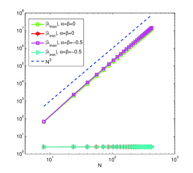
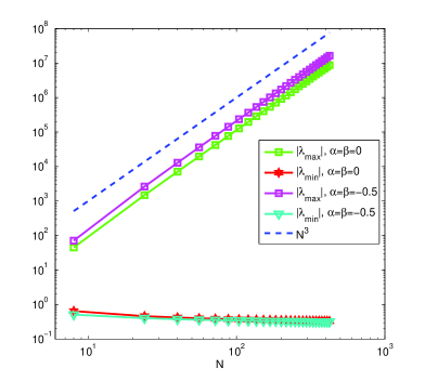
Figure 3.1. Maximum and minimum (in modulus) eigenvalues of F-PSDM with $\mu=1.5$. Left: Caputo. Right: modified Riemann-Liouville.

4. Caputo fractional Birkhoff interpolation and inverse F-PSDM

As already mentioned, the condition number of the collocation system of a FDE of order $\mu$ grows like $O(N^{2\mu}),$ so its solution suffers from severe round-off errors, and it also becomes rather prohibitive to solve the linear system by an iterative method. Following the spirit of [10, 46], we introduce the Caputo fractional Birkhoff interpolation that generates a new interpolating polynomial basis with remarkable properties:

• It provides a stable way to invert the Caputo F-PSDM in (3.38), leading to optimal fractional integration preconditioners for the ill-conditioned collocation schemes.

• It offers a basis for constructing well-conditioned collocation schemes.

4.1. Caputo fractional Birkhoff interpolation

Let $\big{\{}x_{j}=x_{N,j}^{(\alpha,\beta)}\big{\}}_{j=0}^{N}$ (with $x_{0}=-1$ and $x_{N}=1$) be the JGL points as before. Consider the following two interpolating problems:

• For $\mu\in(0,1)$, the Caputo fractional Birkhoff interpolation is to find $p\in{\mathcal{P}}_{N}$ such that

  $${}^{C}{D}^{\mu}_{-}\,p(x_{j})={}^{C}{D}^{\mu}_{-}u(x_{j}),\;\;1\leq j\leq N;\quad p(-1)=u(-1),$$ (4.1)

  for any $u\in C[-1,1]$ satisfying ${}^{C}{D}^{\mu}_{-}u\in C(-1,1].$

• For $\mu\in(1,2)$, the Caputo fractional Birkhoff interpolation is to find $p\in{\mathcal{P}}_{N}$ such that

  $${}^{C}{D}^{\mu}_{-}\,p(x_{j})={}^{C}{D}^{\mu}_{-}u(x_{j}),\;\;1\leq j\leq N-1;\quad p(\pm 1)=u(\pm 1),$$ (4.2)

  for any $u\in C[-1,1]$ satisfying ${}^{C}{D}^{\mu}_{-}u\in C(-1,1).$

Remark 4.1.

The usual Birkhoff interpolation is comprehensively studied in e.g., the monograph [33]. Typically, a polynomial Birkhoff interpolation requires at least one point at which the function and the derivative values are not interpolated consecutively. For example, consider a three-point interpolation problem: find $p\in{\mathcal{P}}_{2}$ such that

$$p(-1)=u(-1),\quad p^{\prime}(0)=u^{\prime}(0),\quad p(1)=u(1).$$

It defines a Birkhoff interpolation problem, since the function value at $x=0$ is not interpolated, as opposite to the Hermite interpolation. Due to the involvement of Caputo fractional derivatives, we call (4.1) and (4.2) the Caputo fractional Birkhoff interpolation problems. ∎

As with the Lagrange interpolation, we search for a nodal basis to represent the interpolating polynomial $p$. More precisely, we look for $Q_{j}^{\mu}\in{\mathcal{P}}_{N}$ such that

• for $\mu\in(0,1),$

  $${}^{C}{D}^{\mu}_{-}\,Q_{j}^{\mu}(x_{i})=\delta_{ij},\;\;\;1\leq i\leq N;\quad Q_{j}^{\mu}(-1)=0,\quad 1\leq j\leq N,$$ (4.3)

  with $Q_{0}^{\mu}=1;$

• for $\mu\in(1,2),$

  $${}^{C}{D}^{\mu}_{-}\,Q_{j}^{\mu}(x_{i})=\delta_{ij},\;\;\;1\leq i\leq N-1;\quad Q_{j}^{\mu}(\pm 1)=0,\quad 1\leq j\leq N-1,$$ (4.4)

  with $Q_{0}^{\mu}(x)=(1-x)/2$ and $Q_{N}^{\mu}(x)=(1+x)/2.$

Then, we can express the Caputo fractional Birkhoff interpolating polynomial $p$ of (4.1) and (4.2), respectively, as

$$p(x)=u(-1)+\sum_{j=1}^{N}{}^{C}{D}^{\mu}_{-}u(x_{j})\,Q_{j}^{\mu}(x),\quad\mu\in(0,1),$$ (4.5)

and

$$p(x)=\frac{1-x}{2}u(-1)+\sum_{j=1}^{N-1}{}^{C}{D}^{\mu}_{-}u(x_{j})\,Q_{j}^{\mu}(x)+\frac{1+x}{2}u(1),\quad\mu\in(1,2).$$ (4.6)

Therefore, $\{Q_{j}^{\mu}\}$ are dubbed as the Caputo fractional Birkhoff interpolating basis polynomials of order $\mu$.

Introduce the matrices

$${\boldsymbol{Q}}^{(\mu)}=\begin{cases}\big{(}{\boldsymbol{Q}}^{(\mu)}_{lj}\big{)}_{1\leq l,j\leq N},\quad&{\rm if}\;\;\mu\in(0,1),\\[4.0pt] \big{(}{\boldsymbol{Q}}^{(\mu)}_{lj}\big{)}_{1\leq l,j\leq N-1},\quad&{\rm if}\;\;\mu\in(1,2),\end{cases}\quad{\rm where}\;\;\;{\boldsymbol{Q}}^{(\mu)}_{lj}=Q_{j}^{\mu}(x_{l}).$$ (4.7)

Remarkably, the matrix ${\boldsymbol{Q}}^{(\mu)}$ is the inverse of ${}^{C}{\boldsymbol{D}}_{\rm in}^{(\mu)}$ defined in (3.38).

Theorem 4.1.

For $\mu\in(k-1,k)$ with $k=1,2,$ we have

$${\boldsymbol{Q}}^{(\mu)}\,{}^{C}{\boldsymbol{D}}_{\rm in}^{(\mu)}={}^{C}{\boldsymbol{D}}_{\rm in}^{(\mu)}\,{\boldsymbol{Q}}^{(\mu)}={\boldsymbol{I}}_{N+1-k},$$ (4.8)

where ${\boldsymbol{I}}_{N+1-k}$ is the identity matrix of order $N+1-k.$

Proof.

We just prove (4.8) with $\mu\in(0,1),$ as the case $\mu\in(1,2)$ can be shown in a similar fashion. Since $Q_{j}^{\mu}\in{\mathcal{P}}_{N}$ and $Q_{j}^{\mu}(-1)=0$ for $1\leq j\leq N,$ we can write

$$Q_{j}^{\mu}(x)=\sum_{l=0}^{N}Q^{\mu}_{j}(x_{l})h_{l}(x)=\sum_{l=1}^{N}Q^{\mu}_{j}(x_{l})h_{l}(x),\;\;\;1\leq j\leq N,$$

where $\{h_{l}\}$ are the Lagrange interpolating basis polynomials associated with JGL points. Thus,

$${}^{C}{D}^{\mu}_{-}\,Q^{\mu}_{j}(x)=\sum_{l=1}^{N}Q^{\mu}_{j}(x_{l}){}^{C}{D}^{\mu}_{-}\,h_{l}(x).$$

Taking $x=x_{i}$ for $1\leq i\leq N$ in the above equation, we obtain (4.8) with $\mu\in(0,1)$ from (4.3) straightforwardly. ∎

4.2. Computing the new basis $\{Q^{\mu}_{j}\}$

The following property plays a crucial role in computing the new basis $\{Q^{\mu}_{j}\},$ which follows from Lemma 3.1.

Lemma 4.1.

Let $\{x_{j}\}_{j=0}^{N}$ be the JGL points with $x_{0}=-1$ and $x_{N}=1$. Then for $\mu\in(k-1,k)$ with $k=1,2,$ we have

$$D^{k}Q^{\mu}_{j}(x)={}^{R}{D}^{k-\mu}_{-}\,\Big{\{}\Big{(}\frac{1+x}{1+x_{j}}\Big{)}^{k-\mu}\hbar_{j}(x)\Big{\}},\;\;\;1\leq j\leq N+1-k,$$ (4.9)

where $\{\hbar_{j}\}_{j=1}^{N+1-k}$ are the Lagrange-Gauss interpolating basis polynomials associated with the JGL points $\{x_{j}\}_{j=1}^{N+1-k},$ that is,

$$\hbar_{j}\in{\mathcal{P}}_{N-k},\quad\hbar_{j}(x_{i})=\delta_{ij}\;\;\;{\rm for}\;\;\;1\leq i,j\leq N+1-k.$$ (4.10)

Proof.

Since $Q_{j}^{\mu}\in{\mathcal{P}}_{N},$ we obtain from Lemma 3.1 that ${}^{C}{D}^{\mu}_{-}\,Q^{\mu}_{j}\in{\mathcal{F}}_{N-k}^{(k-\mu)}.$ Noting that $\{\hbar_{j}\}_{j=1}^{N+1-k}$ forms a basis of ${\mathcal{P}}_{N-k},$ so by (3.3),

$${}^{C}{D}^{\mu}_{-}\,Q^{\mu}_{j}(x)=\sum_{l=1}^{N+1-k}c_{lj}\;(1+x)^{k-\mu}\hbar_{l}(x),\quad 1\leq j\leq N+1-k.$$

Letting $x=x_{i}$ and using the interpolating conditions, we find that $c_{lj}=(1+x_{l})^{\mu-k}\delta_{lj}.$ Thus, we obtain

$${}^{C}{D}^{\mu}_{-}\,Q^{\mu}_{j}(x)=\Big{(}\frac{1+x}{1+x_{j}}\Big{)}^{k-\mu}\hbar_{j}(x),\;\;\;1\leq j\leq N+1-k.$$ (4.11)

By the definition (2.3), we have ${}^{C}{D}^{\mu}_{-}=I_{-}^{k-\mu}D^{k},$ so using (2.9), we obtain (4.9) from (4.11) immediately. ∎

With the aid of (4.9), we are able to derive the explicit formulas for computing the new basis. We provide the derivation in Appendix B.

Theorem 4.2.

Let $\big{\{}x_{j}=x_{N,j}^{(\alpha,\beta)},\omega_{j}=\omega_{N,j}^{(\alpha,\beta)}\big{\}}_{j=0}^{N}$ with ($\alpha,\beta>-1$ and $x_{0}=-x_{N}=-1$) be the JGL quadrature nodes and weights. Then $\{Q_{j}^{\mu}\}$ can be computed by

• For $\mu\in(0,1),$

  $$Q_{j}^{\mu}(x)=\frac{1}{(1+x_{j})^{1-\mu}}\sum_{l=0}^{N-1}\frac{\Gamma(l-\mu+2)}{l!}\,\breve{\xi}_{lj}\,\int_{-1}^{x}P_{l}(x)dx,\quad 1\leq j\leq N,$$ (4.12)

  where

  $$\breve{\xi}_{lj}=\sum_{n=l}^{N-1}{}^{(\alpha,\beta)\!}\boldsymbol{C}_{ln}^{(\mu-1,1-\mu)}\xi_{nj},$$ (4.13)

  $$\xi_{nj}=\frac{1}{\gamma_{n}^{(\alpha,\beta)}}\bigg{\{}-\frac{c_{j}}{\beta+1}\frac{P_{N}^{(\alpha,\beta)}(-1)}{P_{N}^{(\alpha,\beta)}(x_{j})}P_{n}^{(\alpha,\beta)}(-1)\omega_{0}+P_{n}^{(\alpha,\beta)}(x_{j})\omega_{j}\bigg{\}},$$ (4.14)

  with $c_{j}=1$ for $1\leq j\leq N-1,$ and $c_{N}=\alpha+1.$

• For $\mu\in(1,2),$

  $$Q^{\mu}_{j}(x)=\frac{1}{(1+x_{j})^{2-\mu}}\sum^{N-2}_{l=0}\frac{\Gamma(l-\mu+3)}{l!}\;\breve{\xi}_{lj}\,\Phi_{l}(x),\;\;\;1\leq j\leq N-1,$$ (4.15)

  where

  $$\breve{\xi}_{lj}=\sum_{n=l}^{N-2}{}^{(\alpha,\beta)\!}\boldsymbol{C}_{ln}^{(\mu-2,2-\mu)}\xi_{nj},$$ (4.16)

  $$\xi_{nj}=\frac{1}{\gamma_{n}^{(\alpha,\beta)}}\bigg{\{}\frac{(x_{j}-1)P_{N}^{(\alpha,\beta)}(-1)}{2(\beta+1)P_{N}^{(\alpha,\beta)}(x_{j})}P_{n}^{(\alpha,\beta)}(-1)\omega_{0}$$

  $$\qquad\;\;-\frac{(1+x_{j})P_{N}^{(\alpha,\beta)}(1)}{2(\alpha+1)P_{N}^{(\alpha,\beta)}(x_{j})}P_{n}^{(\alpha,\beta)}(1)\omega_{N}+P_{n}^{(\alpha,\beta)}(x_{j})\omega_{j}\bigg{\}},$$ (4.17)

  and

  $$\Phi_{l}(x):=\frac{1+x}{2}\int_{-1}^{1}(t-1)P_{l}(t)\,dt+\int_{-1}^{x}(x-t)P_{l}(t)\,dt.$$ (4.18)

Here, $\big{\{}{}^{(\alpha,\beta)\!}\boldsymbol{C}_{ln}^{(\mu-k,k-\mu)}\big{\}}$ are the connection coefficients as defined in (2.31).

Remark 4.2.

Observe from (4.13) and (4.16) that if we take $(\alpha,\beta)=(\mu-k,k-\mu)$ with $k=1,2,$ we have $\breve{\xi}_{lj}=\xi_{lj},$ so (4.12) and (4.15) have the simplest form. Thus, it is preferable to choose these special parameters. ∎

5. Modifed RL fractional Birkhoff interpolation and inverse F-PSDM

We introduce in this section the fractional Birkhoff interpolation involving modified Riemann-Liouville (RL) fractional derivatives which offers new polynomial bases for well-conditioned collocation methods for solving FDEs with Riemann-Liouville fractional derivatives. Moreover, we are able to stably compute the inverse matrix of ${}^{R}\widehat{\boldsymbol{D}}_{{\rm in}}^{(\mu)}$ defined in (3.39). However, this process appears more involved than the Caputo case in particular for $\mu\in(1,2).$

5.1. Modified Riemann-Liouville fractional Birkhoff interpolation

Like the Caputo case, we consider the modified Riemann-Liouville fractional Birkhoff interpolating problems (i)-(ii) as defined in (4.1)-(4.2) with ${}^{R}\widehat{\boldsymbol{D}}_{-}^{\mu}$ in place of ${}^{C}{\boldsymbol{D}}_{-}^{\mu}.$ Similarly, we look for the interpolating basis polynomials $\{\widehat{Q}_{j}^{\mu}\}_{j=0}^{N}\subseteq{\mathcal{P}}_{N}$ such that

• for $\mu\in(0,1),$

  $$\begin{split}&{}^{R}\widehat{D}_{-}^{\mu}\,\widehat{Q}_{0}^{\mu}(x_{i})=0,\;\;\;\;\;1\leq i\leq N;\quad\widehat{Q}_{0}^{\mu}(-1)=1,\\ &{}^{R}\widehat{D}_{-}^{\mu}\,\widehat{Q}_{j}^{\mu}(x_{i})=\delta_{ij},\;\;\;1\leq i\leq N,\quad\widehat{Q}_{j}^{\mu}(-1)=0,\quad 1\leq j\leq N;\end{split}$$ (5.1)

• for $\mu\in(1,2),$

  $$\begin{split}&{}^{R}\widehat{D}_{-}^{\mu}\,\widehat{Q}_{0}^{\mu}(x_{i})=0,\;\;\;\;\;1\leq i\leq N-1;\quad\widehat{Q}_{0}^{\mu}(-1)=1,\quad\widehat{Q}_{0}^{\mu}(1)=0,\\ &{}^{R}\widehat{D}_{-}^{\mu}\,\widehat{Q}_{j}^{\mu}(x_{i})=\delta_{ij},\;\;\;1\leq i\leq N-1,\quad\widehat{Q}_{j}^{\mu}(\pm 1)=0,\quad 1\leq j\leq N-1,\\ &{}^{R}\widehat{D}_{-}^{\mu}\,\widehat{Q}_{N}^{\mu}(x_{i})=0,\;\;\;\;\;1\leq i\leq N-1;\quad\widehat{Q}_{N}^{\mu}(-1)=0,\quad\widehat{Q}_{N}^{\mu}(1)=1.\end{split}$$ (5.2)

Then for any $u\in{\mathcal{P}}_{N},$ we can write

$$\begin{split}u(x)&=u(-1)\widehat{Q}_{0}^{\mu}(x)+\sum_{j=1}^{N}{}^{R}\widehat{D}_{-}^{\mu}u(x_{j})\,\widehat{Q}_{j}^{\mu}(x)\qquad\text{(for $\mu\in(0,1)$)}\\ &=u(-1)\widehat{Q}_{0}^{\mu}(x)+\sum_{j=1}^{N-1}{}^{R}\widehat{D}_{-}^{\mu}u(x_{j})\,\widehat{Q}_{j}^{\mu}(x)+u(1)\widehat{Q}_{N}^{\mu}(x)\quad\text{(for $\mu\in(1,2)$)}.\end{split}$$ (5.3)

Introduce the matrices generated from the new basis:

$$\widehat{\boldsymbol{Q}}^{(\mu)}=\begin{cases}\big{(}\widehat{\boldsymbol{Q}}^{(\mu)}_{lj}\big{)}_{1\leq l,j\leq N},\quad&{\rm if}\;\;\mu\in(0,1),\\[4.0pt] \big{(}\widehat{\boldsymbol{Q}}^{(\mu)}_{lj}\big{)}_{1\leq l,j\leq N-1},\quad&{\rm if}\;\;\mu\in(1,2),\end{cases}\quad{\rm where}\;\;\;\widehat{\boldsymbol{Q}}^{(\mu)}_{lj}=\widehat{Q}_{j}^{\mu}(x_{l}).$$ (5.4)

Like Theorem 4.1, we can claim that $\widehat{\boldsymbol{Q}}^{(\mu)}$ is the inverse of ${}^{R}\widehat{\boldsymbol{D}}_{{\rm in}}^{(\mu)}.$ As the proof of the theorem below is very similar to that of Theorem 4.1, we omit it.

Theorem 5.1.

For $\mu\in(k-1,k)$ with $k=1,2,$ we have

$$\widehat{\boldsymbol{Q}}^{(\mu)}{}^{R}{\widehat{\boldsymbol{D}}}^{(\mu)}_{\rm in}={}^{R}{\widehat{\boldsymbol{D}}}^{(\mu)}_{\rm in}\,\widehat{\boldsymbol{Q}}^{(\mu)}=\boldsymbol{I}_{N+1-k},$$ (5.5)

where $\boldsymbol{I}_{N+1-k}$ is the identity matrix of order $N+1-k$.

5.2. Computing the new basis $\big{\{}\widehat{Q}^{\mu}_{j}\big{\}}_{j=0}^{N}$

The following lemma is very useful for the computation, whose proof is provided in Appendix C.

Lemma 5.1.

Let $\mu\in(k-1,k)$ with $k=1,2.$ Then for any $f\in{}_{0}{\mathcal{P}}_{N},$ the fractional equation

$${{}^{R}}{\widehat{D}}^{\mu}_{-}u(x)=f(x),\quad u(-1)=0,$$ (5.6)

has a unique solution $u\in{}_{0}{\mathcal{P}}_{N}$ of the form

$$u(x)=I_{-}^{\mu}\big{\{}(1+x)^{-\mu}f(x)\big{\}}.$$ (5.7)

In particular, for any $u\in{\mathcal{P}}_{N},$ we have

$${{}^{R}}{\widehat{D}}^{\mu}_{-}u(-1)=0\;\;\;\text{if and only if}\;\;\;u(-1)=0.$$ (5.8)

For clarity of presentation, we deal with two cases: (i) $\mu\in(0,1)$ and (ii) $\mu\in(1,2),$ separately.

5.2.1. $\big{\{}\widehat{Q}^{\mu}_{j}\big{\}}_{j=0}^{N}$ with $\mu\in(0,1)$

Using the properties (3.11) and (5.8), we obtain from the interpolating conditions in (5.1) that

$$\big{(}{}^{R}\widehat{D}_{-}^{\mu}\,\widehat{Q}_{j}^{\mu}\big{)}(x)=h_{j}(x),\;\;\;1\leq j\leq N;\quad\big{(}{}^{R}\widehat{D}_{-}^{\mu}\,\widehat{Q}_{0}^{\mu}\big{)}(x)=\xi h_{0}(x),$$ (5.9)

where $\{h_{j}\}$ are the JGL interpolating basis polynomials defined in (2.27), and $\xi$ is a constant to be determined by $\widehat{Q}_{0}^{\mu}(-1)=1.$ Note that thanks to (5.8), the condition $\widehat{Q}_{j}^{\mu}(-1)=0$ is built-in, as $h_{j}(-1)=0$ for $1\leq j\leq N.$ We summarise below the explicit representation of the new basis. Once again, we put the proof in Appendix D.

Theorem 5.2.

Let $\big{\{}x_{j}=x_{N,j}^{(\alpha,\beta)},\omega_{j}=\omega_{N,j}^{(\alpha,\beta)}\big{\}}_{j=0}^{N}$ (with $\alpha,\beta>-1$ and $x_{0}=-1$) be the JGL quadrature points and weights. Then $\big{\{}\widehat{Q}_{j}^{\mu}\big{\}}_{j=0}^{N}$ with $\mu\in(0,1)$ can be computed by

$$\widehat{Q}_{j}^{\mu}(x)=\zeta_{j}\sum_{l=0}^{N}\frac{\Gamma(l-\mu+1)}{l!}\,\hat{t}_{lj}\,P_{l}(x)\;\;\;{\rm with}\;\;\;\hat{t}_{lj}=\sum_{n=l}^{N}{}^{(\alpha,\beta)\!}C_{ln}^{(\mu,-\mu)}t_{nj},$$ (5.10)

where $\zeta_{0}=1/\Gamma(1-\mu),$ $\zeta_{j}=1$ for $1\leq j\leq N,$ $\big{\{}{}^{(\alpha,\beta)\!}C_{ln}^{(\mu,-\mu)}\big{\}}$ are the connection coefficients defined in Subsection 2.3, and

$$t_{nj}=\frac{\omega_{j}}{\tilde{\gamma}_{n}^{(\alpha,\beta)}}P_{n}^{(\alpha,\beta)}(x_{j}),$$ (5.11)

with $\tilde{\gamma}_{n}^{(\alpha,\beta)}$ being defined in (2.28).

Remark 5.1.

If $(\alpha,\beta)=(\mu,-\mu)$ with $\mu\in(0,1),$ we have $\hat{t}_{lj}=t_{lj},$ so $\widehat{Q}_{j}^{\mu}$ has the simplest form. ∎

5.2.2. $\big{\{}\widehat{Q}^{\mu}_{j}\big{\}}_{j=0}^{N}$ with $\mu\in(1,2)$

It is essential to derive the identities like (5.9). Indeed, using (3.11) and (5.8), we obtain from the interpolating conditions in (5.2) that

$$\big{(}{}^{R}\widehat{D}_{-}^{\mu}\,\widehat{Q}_{0}^{\mu}\big{)}(x)=(\tau_{0}+\kappa_{0}\,x)\hat{h}_{0}(x),\quad\widehat{Q}_{0}^{\mu}(-1)=1,\quad\widehat{Q}_{0}^{\mu}(1)=0;$$ (5.12)

$$\big{(}{}^{R}\widehat{D}_{-}^{\mu}\,\widehat{Q}_{j}^{\mu}\big{)}(x)=\frac{x+\tau_{j}}{x_{j}+\tau_{j}}\hat{h}_{j}(x),\quad\widehat{Q}_{j}^{\mu}(1)=0,\quad 1\leq j\leq N-1;$$ (5.13)

$$\big{(}{}^{R}\widehat{D}_{-}^{\mu}\,\widehat{Q}_{N}^{\mu}\big{)}(x)=\tau_{N}(1+x)\,\hat{h}_{0}(x),\quad\widehat{Q}_{N}^{\mu}(1)=1,$$ (5.14)

where $\{\hat{h}_{j}\}_{j=0}^{N-1}$ are the Lagrange interpolating basis polynomials at JGL points $\{x_{j}\}_{j=0}^{N-1},$ that is,

$$\hat{h}_{j}(x)\in{\mathcal{P}}_{N-1},\quad\hat{h}_{j}(x_{i})=\delta_{ij},\quad 0\leq i,j\leq N-1.$$ (5.15)

In (5.12)-(5.14), $\{\tau_{j}\}_{j=0}^{N}$ and $\kappa_{0}$ are constants to be determined by the corresponding conditions at $x=\pm 1$, e.g., $\widehat{Q}_{j}^{\mu}(1)=0$ in (5.13). It is noteworthy that thanks to (5.8), the interpolating condition: $\widehat{Q}_{j}^{\mu}(-1)=0$ is built in $\big{(}{}^{R}\widehat{D}_{-}^{\mu}\,\widehat{Q}_{j}^{\mu}\big{)}(-1)=0$ for $1\leq j\leq N.$

In what follows, we shall use the three-term recurrence relation of Jacobi polynomials (cf. [39, (3.110)]):

$$xP^{(\mu,1-\mu)}_{l}(x)=a_{l+1}P^{(\mu,1-\mu)}_{l+1}(x)+b_{l}P^{(\mu,1-\mu)}_{l}(x)+c_{l-1}P^{(\mu,1-\mu)}_{l-1}(x),\quad l\geq 0,$$ (5.16)

where $c_{-1}=0,$ $\mu\in(1,2),$ and

$$a_{l+1}=\displaystyle\frac{l+2}{2l+3},\quad b_{l}=\displaystyle\frac{1-2\mu}{(2l+1)(2l+3)},\quad c_{l-1}=\displaystyle\frac{(l+\mu)(l-\mu+1)}{(l+1)(2l+1)}.$$ (5.17)

As before, it is necessary to expand $\{\hat{h}_{j}\}$ in terms of Jacobi polynomials with different parameters by using the notion of connection problems, so as to use compact and closed-form formulas to compute the new basis. We state below the connections of three expansions, and postpone the derivations in Appendix E.

Lemma 5.2.

Let $\big{\{}x_{j}=x_{N,j}^{(\alpha,\beta)},\omega_{j}=\omega_{N,j}^{(\alpha,\beta)}\big{\}}_{j=0}^{N}$ (with $\alpha,\beta>-1$ and $x_{0}=-x_{N}=-1$) be the JGL quadrature nodes and weights, and let $\{\hat{h}_{j}\}_{j=0}^{N-1}$ be the Lagrange interpolating basis polynomials associated with $\{x_{j}\}_{j=0}^{N-1}$ defined in (5.15). Then for $\mu\in(1,2),$ we have

$$\begin{split}\hat{h}_{j}(x)&=\sum_{n=0}^{N-1}\varrho_{nj}\,P_{n}^{(\alpha,\beta)}(x)=\sum_{l=0}^{N-1}\tilde{\varrho}_{lj}\,P_{l}^{(\mu,1-\mu)}(x)\\ &=\hat{\varrho}_{0j}+\sum_{l=0}^{N-2}\hat{\varrho}_{l+1,j}\,(1+x)P_{l}^{(\mu,1-\mu)}(x),\;\;0\leq j\leq N-1,\end{split}$$ (5.18)

where $\hat{\varrho}_{00}=1$ and $\hat{\varrho}_{0j}=0$ for $1\leq j\leq N-1.$ Moreover, the coefficients can be computed by

$$\varrho_{n0}=\frac{1}{\gamma_{n}^{(\alpha,\beta)}}\Big{\{}P_{n}^{(\alpha,\beta)}(-1)\omega_{0}-\frac{\beta+1}{\alpha+1}\frac{P_{N}^{(\alpha,\beta)}(1)}{P_{N}^{(\alpha,\beta)}(-1)}P_{n}^{(\alpha,\beta)}(1)\omega_{N}\Big{\}},$$ (5.19)

$$\varrho_{nj}=\frac{1}{\gamma_{n}^{(\alpha,\beta)}}\Big{\{}P_{n}^{(\alpha,\beta)}(x_{j})\omega_{j}-\frac{1}{\alpha+1}\frac{P_{N}^{(\alpha,\beta)}(1)}{P_{N}^{(\alpha,\beta)}(x_{j})}P_{n}^{(\alpha,\beta)}(1)\omega_{N}\Big{\}},\;\;\;1\leq j\leq N-1,$$ (5.20)

$$\tilde{\varrho}_{lj}=\sum_{n=l}^{N-1}{}^{(\alpha,\beta)\!}C_{ln}^{(\mu,1-\mu)}\varrho_{nj},\quad 0\leq l,j\leq N-1,$$ (5.21)

and by the backward recurrence relation:

$$\begin{split}&\hat{\varrho}_{ij}=\frac{1}{a_{i}}\tilde{\varrho}_{ij}-\frac{b_{i}+1}{a_{i}}\hat{\varrho}_{i+1,j}-\frac{c_{i}}{a_{i}}\hat{\varrho}_{i+2,j},\quad i=N-3,N-2,\cdots,1,\\ &\hat{\varrho}_{N-1,j}=\frac{1}{a_{N-1}}\tilde{\varrho}_{N-1,j},\quad\hat{\varrho}_{N-2,j}=\frac{1}{a_{N-2}}\tilde{\varrho}_{N-2,j}-\frac{b_{N-2}+1}{a_{N-2}}\hat{\varrho}_{N-1,j},\end{split}$$ (5.22)

where $\{a_{i},b_{i},c_{i}\}$ are given in (5.17).

With the above preparations, we are ready to derive the explicit formulas of the new basis $\big{\{}\widehat{Q}_{j}^{\mu}\big{\}}_{j=0}^{N}$ with $\mu\in(1,2).$ We refer to Appedix F for the derivation.

Theorem 5.3.

Let $\big{\{}\tilde{\varrho}_{lj},\hat{\varrho}_{lj}\big{\}}$ be the coefficients defined in Lemma 5.2, and denote

$$d_{l}^{\mu}:=\frac{\Gamma(l+2-\mu)}{(l+1)!},\quad\varphi_{l}(x):=(1+x)P_{l}^{(0,1)}(x).$$ (5.23)

Then $\big{\{}\widehat{Q}_{j}^{\mu}\big{\}}_{j=0}^{N}$ at JGL points with $\mu\in(1,2)$ can be computed by

• for $j=0,$

  $$\begin{split}\widehat{Q}_{0}^{\mu}(x)=&1+\Big{(}\tau_{0}-\frac{1}{\Gamma(1-\mu)}\Big{)}\sum_{l=0}^{N-1}d_{l}^{\mu}\tilde{\varrho}_{l0}\,\varphi_{l}(x)+\frac{1}{\Gamma(1-\mu)}\sum_{l=0}^{N-2}d_{l}^{\mu}\hat{\varrho}_{l+1,0}\,\varphi_{l}(x),\\ {\rm where}\;\;&\;\;\tau_{0}-\frac{1}{\Gamma(1-\mu)}=-\bigg{\{}\frac{1}{2}+\frac{1}{\Gamma(1-\mu)}\sum_{l=0}^{N-2}d_{l}^{\mu}\hat{\varrho}_{l+1,0}\,\bigg{\}}\bigg{/}\sum_{l=0}^{N-1}d_{l}^{\mu}\tilde{\varrho}_{l0};\end{split}$$ (5.24)

• for $j=N,$

  $$\widehat{Q}_{N}^{\mu}(x)=\frac{1}{2}\sum_{l=0}^{N-1}d_{l}^{\mu}\tilde{\varrho}_{l0}\,\varphi_{l}(x)\bigg{/}\sum_{l=0}^{N-1}d_{l}^{\mu}\tilde{\varrho}_{l0}\,;$$ (5.25)

• for $1\leq j\leq N-1,$

  $$\begin{split}&\widehat{Q}_{j}^{\mu}(x)=\frac{\tau_{j}}{x_{j}+\tau_{j}}\sum_{l=0}^{N-2}d_{l}^{\mu}\hat{\varrho}_{l+1,j}\,\varphi_{l}(x)+\frac{1}{x_{j}+\tau_{j}}\\ &\quad\times\sum_{l=0}^{N-2}d_{l}^{\mu}\hat{\varrho}_{l+1,j}\,\bigg{\{}\frac{l+2-\mu}{l+2}a_{l+1}\varphi_{l+1}(x)+b_{l}\varphi_{l}(x)+\frac{l+1}{l+1-\mu}c_{l-1}\varphi_{l-1}(x)\bigg{\}},\\ \end{split}$$ (5.26)

  where $\{a_{l},b_{l},c_{l}\}$ (with $c_{-1}=0{\rm)}$ are defined in (5.17), and

  $$\tau_{j}=-1+\mu\,\Gamma(2-\mu)\hat{\varrho}_{1j}\bigg{/}{\sum_{l=0}^{N-2}d_{l}^{\mu}\hat{\varrho}_{l+1,j}}.$$ (5.27)

Remark 5.2.

We see from (5.21) that if $(\alpha,\beta)=(\mu,1-\mu)$ with $\mu\in(1,2),$ the connections coefficients are not involved, so $\widehat{Q}_{j}^{\mu}$ has simpler form. ∎

6. Well-conditioned collocation schemes and numerical results

In this section, we apply the tools developed in previous sections to construct well-conditioned collocation schemes for initial-valued or boundary-valued FDEs, and provide ample numerical results to show the accuracy and stability of the methods.

6.1. Initial-valued Caputo FDEs

To fix the idea, we first consider the Caputo FDE of order $\mu\in(0,1):$

$${{}^{C}}D_{-}^{\mu}u(x)+\lambda(x)u(x)=f(x),\quad x\in(-1,1];\quad u(-1)=u_{-},$$ (6.1)

where $\lambda,f$ are given continuous functions, and $u_{-}$ is a given constant. The collocation scheme is to find $u_{N}\in{\mathcal{P}}_{N}$ such that

$${{}^{C}}D_{-}^{\mu}u_{N}(x_{j})+\lambda(x_{j})u_{N}(x_{j})=f(x_{j}),\quad 1\leq j\leq N;\quad u_{N}(-1)=u_{-}.$$ (6.2)

The corresponding linear system under the Lagrange basis polynomials $\{h_{j}\}$ (L-COL) becomes

$$\big{(}{}^{C}{\boldsymbol{D}}_{\rm in}^{(\mu)}+\boldsymbol{\Lambda}\big{)}\boldsymbol{u}=\boldsymbol{f},$$ (6.3)

where ${}^{C}{\boldsymbol{D}}_{\rm in}^{(\mu)}$ is defined as in (3.38), $\boldsymbol{\Lambda}={\rm diag}(\lambda(x_{1}),\cdots,\lambda(x_{N})),$ and

$$\boldsymbol{u}=\big{(}u_{N}(x_{1}),\cdots,u_{N}(x_{N})\big{)}^{t},\;\;\boldsymbol{f}=\big{(}f(x_{1})-u_{-}{{}^{C}}D_{-}^{\mu}h_{0}(x_{1}),\cdots,f(x_{N})-u_{-}{{}^{C}}D_{-}^{\mu}h_{0}(x_{N})\big{)}^{t}.$$ (6.4)

The collocation system under the Birkhoff interpolation basis polynomials $\{Q_{j}^{\mu}\}$ in (4.3) (B-COL) becomes

$$\big{(}\boldsymbol{I}_{N}+\boldsymbol{\Lambda}\boldsymbol{Q}^{(\mu)}\big{)}\boldsymbol{v}=\boldsymbol{g},$$ (6.5)

where

$$u_{N}(x)=u_{-}+\sum_{i=1}^{N}v_{j}Q_{j}^{\mu}(x),\quad\boldsymbol{v}=\big{(}v_{1},\cdots,v_{N}\big{)}^{t},$$ (6.6)

and $\boldsymbol{g}=\big{(}f(x_{1})-u_{-}\lambda(x_{1}),\cdots,f(x_{N})-u_{-}\lambda(x_{N})\big{)}^{t}$. It is noteworthy that different from (6.3), the unknowns of (6.5) are not the approximation of $u$ at the collocation points, but of the Caputo fractional derivative values in view of (4.5).

Thanks to Theorem 4.1, we can precondition (6.3) and obtain the PL-COL system:

$$\big{(}\boldsymbol{I}_{N}+\boldsymbol{Q}^{(\mu)}\boldsymbol{\Lambda}\big{)}\boldsymbol{u}=\boldsymbol{Q}^{(\mu)}\boldsymbol{f}.$$ (6.7)

In the computation, we take $\lambda(x)=2+\sin(25x)$ and $u(x)=E_{\mu,1}(-2(1+x)^{\mu})$ with $\mu=0.8$ in (6.1), where the Mittag-Leffler function is defined by

$$E_{\alpha,\beta}(z)=\sum_{n=0}^{\infty}\frac{z^{n}}{\Gamma(n\alpha+\beta)}.$$ (6.8)

In view of Remark 4.2, we choose the JGL points with $(\alpha,\beta)=(\mu-1,1-\mu)=(-0.2,0.2).$ We compare the condition numbers, number of iterations (using BiCGSTAB in Matlab) and convergence behaviour (in discrete $L^{2}$-norm on fine equally-spaced grids) of three schemes (see Figure 6.1). Observe from Figure 6.1 (left) that the condition number of usual L-COL divided by $N^{2\mu}$ behaves like a constant, while that of PL-COL and B-COL remains a constant even for $N$ up to $2000.$ As a result, the latter two schemes only require about $8$ iterations to converge, while the usual L-COL scheme requires much more iterations with a degradation of accuracy as depicted in Figure 6.1 (middle). We record the convergence history of three methods in Figure 6.1 (right), and observe that two new schemes are stable even for very large $N.$

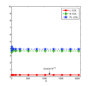
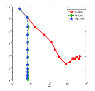
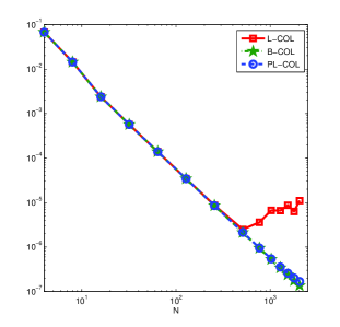
Figure 6.1. Comparison of condition numbers (left), iteration numbers against errors (middle), and errors against $N$ at convergence in log-log scale (right) for (6.1).

6.2. Boundary-valued Caputo FDEs

We now turn to the boundary value problem:

$$\begin{split}&{{}^{C}}D_{-}^{\mu}u(x)+\lambda_{1}(x){{}^{C}}D_{-}^{\nu}u(x)+\lambda_{2}(x)u(x)=f(x),\quad x\in(-1,1);\\ &u(-1)=u_{-},\quad u(1)=u_{+},\quad 0<\nu<\mu,\;\;\;\mu\in(1,2),\end{split}$$ (6.9)

where $\lambda_{1},\lambda_{2}$ and $f$ are given continuous functions, and $u_{\pm}$ are given constants.

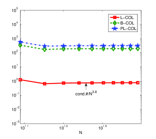
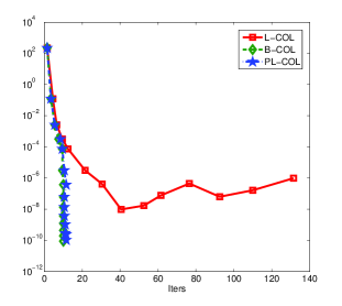
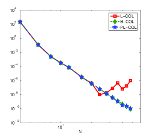
Figure 6.2. Comparison of condition numbers (left), iteration numbers against errors (middle), and errors against $N$ at convergence in log-log scale (right) for (6.9).

With a pre-computation of the Caputo fractional differentiation matrices of order $\mu$ and $\nu$ in Subsection 3.2, we can formulate the L-COL scheme as (6.3) straightforwardly. The counterpart of (6.5) i.e., the B-COL scheme, can be formulated as follows: find (cf. (4.6))

$$u_{N}(x)=u_{N}^{*}(x)+\sum_{j=1}^{N-1}v_{j}\,Q_{j}^{\mu}(x),\quad\mu\in(1,2);\quad u_{N}^{*}(x):=\frac{1-x}{2}u_{-}+\frac{1+x}{2}u_{+},$$ (6.10)

such that

$$\big{(}\boldsymbol{I}_{N-1}+\boldsymbol{\Lambda}_{1}\bar{\boldsymbol{Q}}^{(\nu)}+\boldsymbol{\Lambda}_{2}\boldsymbol{Q}^{(\mu)}\big{)}\boldsymbol{v}=\boldsymbol{g},$$ (6.11)

where $\boldsymbol{\Lambda}_{i}={\rm diag}(\lambda_{i}(x_{1}),\cdots,\lambda_{i}(x_{N-1})),i=1,2,$ $\bar{\boldsymbol{Q}}^{(\nu)}_{ij}={{}^{C}}D_{-}^{\nu}Q_{j}^{\mu}(x_{i}),1\leq i,j\leq N-1,$ and $\boldsymbol{g}=\big{(}f(x_{1})-q_{*}(x_{1}),\cdots,f(x_{N-1})-q_{*}(x_{N-1})\big{)}^{t}$ with $q_{*}=\lambda_{1}{{}^{C}}D_{-}^{\nu}u_{N}^{*}+\lambda_{2}\,u_{N}^{*}.$ Note that the entries of $\bar{\boldsymbol{Q}}^{(\nu)}$ can be evaluated by Theorem 2.1, (2.7) and (4.15)-(4.18). Here, we omit the details.

Remark 6.1.

If $\lambda_{1}=0$ and $\lambda_{2}$ is a constant, we can follow [46, Proposition 3.5] to justify the coefficient matrix of (6.11) is well-conditioned. Indeed, thanks to Theorem 4.1, the eigenvalues $\sigma$ of $\boldsymbol{I}_{N-1}-\lambda_{2}\boldsymbol{Q}^{(\mu)}$ satisfy

$$1+{\lambda_{2}}{\lambda_{\rm max}^{-1}}\leq\sigma\leq 1+{\lambda_{2}}{\lambda_{\rm min}^{-1}},$$

where $\lambda_{\rm max}$ and $\lambda_{\rm min}$ are respectively the largest and smallest eigenvalues of ${}^{C}{\boldsymbol{D}}_{\rm in}^{(\mu)}.$ Since $\lambda_{\rm min}=O(1)$ (see Figure 3.1 (right)), the condition number of $\boldsymbol{I}_{N-1}-\lambda_{2}\boldsymbol{Q}^{(\mu)}$ is independent of $N.$ ∎

Like (6.7), we can precondition the L-COL scheme by ${\boldsymbol{Q}}^{(\mu)}$ which leads to the PL-COL system.

In the following comparison, we set $\mu=1.9,\nu=0.7$ and $(\alpha,\beta)=(-0.1,0.1)$ (cf. Remark 4.2), and take

$$\lambda_{1}(x)=2+\sin(4\pi x),\;\;\;\;\lambda_{2}(x)=2+\cos x,$$ (6.12)

and

$$\;\;u(x)=e^{1+x}+(1+x)^{6+{4}/{7}}-2(1+x)^{5+{4}/{7}},$$ (6.13)

where we can use the formula

$${{}^{C}}D_{-}^{\mu}e^{1+x}=(1+x)^{k-\mu}E_{1,k+1-\mu}(1+x),\quad\mu\in(k-1,k),\;\;k=1,2,$$

to work out $f(x).$

Once again, we observe from Figure 6.2 that the new schemes: B-COL and PL-COL are well-conditioned, attain the expected convergence order about $10$ iterations, and lead to stable computation for large $N.$

6.3. Riemann-Liouville FDEs

Consider the Riemann-Liouville version of (6.9):

$$\begin{split}&{{}^{R}}D_{-}^{\mu}u(x)+\lambda_{1}(x){{}^{R}}D_{-}^{\nu}u(x)+\lambda_{2}(x)u(x)=f(x),\quad x\in(-1,1);\\ &u(-1)=u_{-},\quad u(1)=u_{+},\quad 0<\nu<\mu,\;\;\;\mu\in(1,2),\end{split}$$ (6.14)

where $\lambda_{1},\lambda_{2}$ and $f$ are given continuous functions, and $u_{\pm}$ are given constants.

For a better treatment of the singularity, we consider the modified Riemann-Liouville fractional collocation scheme: find $u_{N}\in{\mathcal{P}}_{N}$ such that

$$\begin{split}&{{}^{R}}\widehat{D}_{-}^{\mu}u_{N}(x_{j})+\hat{\lambda}_{1}(x_{j}){{}^{R}}\widehat{D}_{-}^{\nu}u_{N}(x_{j})+\hat{\lambda}_{2}(x_{j})u_{N}(x_{j})=\hat{f}(x_{j}),\quad 1\leq j\leq N;\\ &u_{N}(-1)=u_{-},\quad u_{N}(1)=u_{+},\quad 0<\nu<\mu,\;\;\mu\in(1,2),\end{split}$$ (6.15)

where $\hat{\lambda}_{1}=(1+x)^{\mu-\nu}\lambda_{1},$ $\hat{\lambda}_{2}=(1+x)^{\mu}\lambda_{2},$ and $\hat{f}=(1+x)^{\mu}f.$

Here, we just focus on the collocation system using the new basis in (5.3), that is,

$$u_{N}(x)=u_{-}\widehat{Q}_{0}^{\mu}(x)+u_{+}\widehat{Q}_{N}^{\mu}(x)+\sum_{j=1}^{N-1}v_{j}\,\widehat{Q}_{j}^{\mu}(x),\quad\mu\in(1,2).$$ (6.16)

Then one can write down the B-COL system in a fashion very similar to (6.11) with only a change of basis. Correspondingly, we denote the matrix of the linear system by $\boldsymbol{A}:=\boldsymbol{I}_{N-1}+\boldsymbol{\Lambda}_{1}\widetilde{\boldsymbol{Q}}^{(\nu)}+\boldsymbol{\Lambda}_{2}\widehat{\boldsymbol{Q}}^{(\mu)}.$

We first show that the B-COL scheme enjoys spectral accuracy (i.e., exponential convergence), when the underlying solution is sufficiently smooth. For this purpose, we take

$$u(x)=e^{-(1+x)}-\frac{1-x}{2}-e^{-2}\frac{1+x}{2},$$ (6.17)

and $\lambda_{1},\lambda_{2}$ to be the same as in (6.12). In Figure 6.3, we plot discrete $L^{2}$-errors for various pairs of $(\mu,\nu)$ of the B-COL schemes for both Caputo and Riemann-Liouville fractional boundary value problems (BVPs) (6.9) and (6.14) under the same setting. We observe the exponential decay (i.e., $O(e^{-cN})$ for some $c>0$) of the errors. Both schemes take about $10$ iterations to converge, while much more iterations are needed and severe round-off errors are induced if one uses the standard L-COL approach.

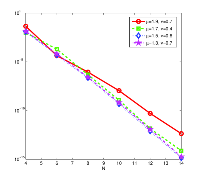
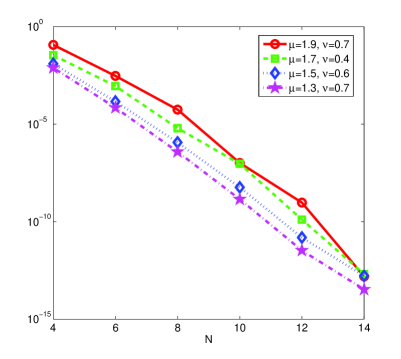
Figure 6.3. Errors against $N$ of the B-COL schemes for Caputo fractional BVP (6.9) (left) and Riemann-Liouville fractional BVP (6.14) (right) with various $\mu,\nu$, where $\lambda_{1},\lambda_{2}$ are given in (6.12), and the exact solution $u$ is given in (6.17).

We further test the new B-COL method on (6.14) with smooth coefficients but large derivative:

$$\lambda_{1}(x)=1+e^{-1000x^{2}},\quad\lambda_{2}(x)=1+e^{-1000(x+0.2)^{2}},$$ (6.18)

and with the exact solution having finite regularity in the usual Sobolev space:

$$u(x)=E_{\mu,1}\big{(}-(1+x)^{\mu}/2\big{)}+\frac{1-E_{\mu,1}(-2^{\mu-1})}{2}(1+x)-1.$$ (6.19)

We tabulate in Table 6.1 the discrete $L^{2}$-errors, number of iterations and the second smallest and largest eigenvalues (in modulus). Once again, the scheme converges within a few iterations even for very large $N.$ In fact, as we observed from Figure 3.1 (right), the smallest eigenvalue of ${}^{R}\widehat{\boldsymbol{D}}_{{\rm in}}^{(\mu)}$ in (3.39) still mildly depends on $N.$ As a result, the condition number of $\boldsymbol{A}$ grows mildly with respect to $N.$ However, it is interesting to find that the eigenvalues in modulus of $\boldsymbol{A}$ (denoted by $\{|\sigma_{j}|\}_{j=1}^{N-1}$ which are arranged in ascending order) are concentrated in the sense that

$$O(1)=|\sigma_{2}|\leq|\sigma_{j}|\leq|\sigma_{N-2}|=O(1),\quad 2\leq j\leq N-2.$$ (6.20)

Thanks to this remarkable property, the iterative solver for the modified Riemann-Liouville system is actually as fast as the previous Caputo system where the coefficient matrix is well-conditioned.

Table 6.1. Errors, number of iterations and concentration of eigenvalues of $\boldsymbol{A}$

$N$	$\mu=1.5,\;\;\nu=0.6$				$\mu=1.9,\;\;\nu=0.7$
	$|\sigma_{2}|$	$|\sigma_{N-2}|$	Iters	Errors	$|\sigma_{2}|$	$|\sigma_{N-2}|$	Iters	Errors
8	0.7	1.0	7	8.58e-03	0.4	1.0	6	2.66e-03
16	0.6	1.1	12	2.03e-03	0.2	1.7	8	3.69e-04
32	0.6	1.2	12	5.39e-04	0.2	3.0	8	5.49e-05
64	0.6	1.3	12	1.31e-04	0.1	5.0	8	7.46e-06
128	0.6	1.5	12	3.24e-05	0.1	7.4	8	1.06e-06
256	0.6	1.6	12	8.08e-06	0.1	9.9	8	1.53e-07
512	0.6	1.7	13	2.02e-06	0.1	12.7	8	2.21e-08
1024	0.6	1.7	13	5.04e-07	0.1	21.1	8	3.69e-09

6.4. Concluding remarks

In this paper, we provided an explicit and compact means for computing Caputo and modified Riemann-Liouville F-PSDMs of any order, and introduced new fractional collocation schemes using fractional Birkhoff interpolation basis functions. We showed that the new approaches significantly outperformed the standard collocation approximation using Lagrange interpolation basis.

As a final remark, we point out two topics worthy of future investigation along this line, which we wish to explore in forthcoming papers. The first is to analyze the fractional Birkhoff interpolation errors and understand the approximability of the new interpolation basis functions from theoretical perspective. The second is to extend the idea and techniques in this paper to study the fractional collocation methods using the nodal basis $\big{\{}(1+x)^{\mu}h_{j}(x)/(1+x_{j})^{\mu}\big{\}}$ (see [50], i.e., the counterpart of Jacobi poly-fractonomials [49] and generalised Jacobi functions [46]).

Appendix A Proof of Theorem 3.2

We expand $\{h_{j}^{\prime}\}$ in terms of Legendre polynomials, and look for $\{s_{lj}\}$ such that

$$h_{j}^{\prime}(x)=\frac{1}{2}\sum_{n=1}^{N}(n+\alpha+\beta+1)t_{nj}P_{n-1}^{(\alpha+1,\beta+1)}(x)=\sum_{l=1}^{N}s_{lj}P_{l-1}(x),\quad 0\leq j\leq N,$$ (A.1)

where $\{t_{nj}\}$ are given in (2.27) and we used the derivative formula (cf. [41]):

$$DP_{n}^{(\alpha,\beta)}(x)=\frac{1}{2}(n+\alpha+\beta+1)P_{n-1}^{(\alpha+1,\beta+1)}(x),\quad n\geq 1.$$ (A.2)

By (2.29)-(2.32), we find that

$$s_{lj}=\frac{1}{2}\sum_{n=1}^{N}(n+\alpha+\beta+1){}^{(\alpha+1,\beta+1)\!}C_{l-1,n-1}^{(0,0)}\,t_{nj}=\frac{1}{2}\sum_{n=l-1}^{N}(n+\alpha+\beta+1){}^{(\alpha+1,\beta+1)\!}C_{l-1,n-1}^{(0,0)}\,t_{nj},$$ (A.3)

for $1\leq l\leq N$ and $0\leq j\leq N.$ In view of (A.1), we can use the first formula in (2.23) to derive

$$\begin{split}{}^{C}{\boldsymbol{D}}^{(\mu)}_{ij}&:=\big{(}{}^{C}{D}^{\mu}_{-}h_{j}\big{)}(x_{i})=I^{1-\mu}_{-}h_{j}^{\prime}(x_{i})=\sum_{l=1}^{N}s_{lj}I^{1-\mu}_{-}P_{l-1}(x_{i})\\ &=(1+x_{i})^{1-\mu}\sum_{l=1}^{N}\frac{(l-1)!}{\Gamma(l+1-\mu)}\,s_{lj}\,P_{l-1}^{(\mu-1,1-\mu)}(x_{i})\,.\end{split}$$ (A.4)

This ends the derivation of (3.22)-(3.23).

We now derive (3.24) for the LGL case. Using the orthogonality of Legendre polynomials, integration by parts and the exactness of LGL quadrature (cf. (2.25)), we obtain from (A.1) that

$$\begin{split}s_{lj}&=\frac{1}{\gamma_{l-1}}\int_{-1}^{1}h_{j}^{\prime}(x)P_{l-1}(x)\,dx=\frac{1}{\gamma_{l-1}}\bigg{\{}h_{j}(x)P_{l-1}(x)\big{|}_{-1}^{1}-\sum_{i=0}^{N}h_{j}(x_{i})P_{l-1}^{\prime}(x_{i})\omega_{i}\bigg{\}}\\ &=\frac{1}{\gamma_{l-1}}\big{\{}\delta_{jN}+(-1)^{l}\delta_{j0}-\omega_{j}P_{l-1}^{\prime}(x_{j})\big{\}},\end{split}$$ (A.5)

where we used the properties: $h_{j}(x_{i})=\delta_{ij}$ and $P_{l-1}(\pm 1)=(\pm 1)^{l-1}.$

Appendix B Proof of Theorem 4.2

Since $\hbar_{j}\in{\mathcal{P}}_{N-k},$ we can write

$$\hbar_{j}(x)=\displaystyle\sum^{N-k}_{n=0}\xi_{nj}P_{n}^{(\alpha,\beta)}(x)=\sum^{N-k}_{l=0}\breve{\xi}_{lj}P^{(\mu-k,k-\mu)}_{l}(x),\;\;\;1\leq j\leq N+1-k.$$ (B.1)

As before, if one can work out $\{\xi_{nj}\},$ then by (2.29)-(2.32),

$$\breve{\xi}_{lj}=\sum_{n=l}^{N-k}{}^{(\alpha,\beta)\!}C_{ln}^{(\mu-k,k-\mu)}\xi_{nj}.$$ (B.2)

As to be shown later, inserting (B.1) into (4.9), we can derive from (2.24) with $\rho=k-\mu$ the desired formulas. Thus, it remains to find $\{\xi_{nj}\}$ in (B.1). We proceed separately for two cases.

(i) For $\mu\in(0,1),$ we obtain from the orthogonality (2.17), the exactness of JGL quadrature (2.25), and the interpolating condition (4.10) that

$$\begin{split}\xi_{nj}&=\frac{1}{\gamma_{n}^{(\alpha,\beta)}}\int^{1}_{-1}\hbar_{j}(x)P_{n}^{(\alpha,\beta)}(x)\omega^{(\alpha,\beta)}(x)dx=\frac{1}{\gamma_{n}^{(\alpha,\beta)}}\sum_{i=0}^{N}\hbar_{j}(x_{i})P_{n}^{(\alpha,\beta)}(x_{i})\omega_{i}\\ &=\frac{1}{\gamma_{n}^{(\alpha,\beta)}}\big{\{}\hbar_{j}(-1)P_{n}^{(\alpha,\beta)}(-1)\omega_{0}+P_{n}^{(\alpha,\beta)}(x_{j})\omega_{j}\big{\}},\quad 1\leq j\leq N.\end{split}$$ (B.3)

Now, we evaluate $\hbar_{j}(-1).$ Since $\{\hbar_{j}\}$ are associated with the interpolating points $\{x_{j}\}_{j=1}^{N},$ which are zeros of $(1-x)DP_{N}^{(\alpha,\beta)}(x),$ we have the representation:

$$\hbar_{j}(x)=\frac{(1-x)DP^{(\alpha,\beta)}_{N}(x)}{(x-x_{j})D\big{\{}(1-x)DP^{(\alpha,\beta)}_{N}(x)\big{\}}\big{|}_{x=x_{j}}},\quad 1\leq j\leq N.$$ (B.4)

Recall the Sturm-Liouville equation of Jacobi polynomials (cf. [41, (4.2.1)]):

$$-(1-x^{2})D^{2}P^{(\alpha,\beta)}_{N}(x)=\big{\{}\beta-\alpha-(\alpha+\beta+2)x\big{\}}DP^{(\alpha,\beta)}_{N}(x)+\lambda^{(\alpha,\beta)}_{N}P^{(\alpha,\beta)}_{N}(x),$$ (B.5)

where $\lambda_{N}^{(\alpha,\beta)}=N(N+\alpha+\beta+1).$ It follows from (B.5) that

$$\begin{split}&2(\beta+1)DP_{N}^{(\alpha,\beta)}(-1)=-\lambda^{(\alpha,\beta)}_{N}P_{N}^{(\alpha,\beta)}(-1),\;\;\;2(\alpha+1)DP_{N}^{(\alpha,\beta)}(1)=\lambda^{(\alpha,\beta)}_{N}P_{N}^{(\alpha,\beta)}(1),\\ &-(1-x^{2}_{j})D^{2}P^{(\alpha,\beta)}_{N}(x_{j})=\lambda^{(\alpha,\beta)}_{N}P^{(\alpha,\beta)}_{N}(x_{j}),\quad 1\leq j\leq N-1.\end{split}$$ (B.6)

Using the property: $(1-x_{j})DP_{N}^{(\alpha,\beta)}(x_{j})=0$ and (B.6), we compute from (B.4) that

$$\hbar_{j}(-1)=-\frac{c_{j}}{\beta+1}\frac{P_{N}^{(\alpha,\beta)}(-1)}{P_{N}^{(\alpha,\beta)}(x_{j})},\;\;\;1\leq j\leq N,$$ (B.7)

where $c_{j}=1$ for $1\leq j\leq N-1,$ and $c_{N}=\alpha+1.$ Substituting (B.7) into (B.3) yields (4.14).

Inserting (B.1) into (4.9), we derive from (2.24) with $\rho=1-\mu$ that

$$DQ_{j}^{\mu}(x)=\frac{1}{(1+x_{j})^{1-\mu}}\sum_{l=0}^{N-1}\frac{\Gamma(l-\mu+2)}{l!}\,\breve{\xi}_{lj}\,P_{l}(x),\quad 1\leq j\leq N.$$ (B.8)

In view of $Q_{j}^{\mu}(-1)=0,$ a direct integration of (B.8) leads to (4.12).

(ii) For $\mu\in(1,2),$ (B.3) reads

$$\begin{split}\xi_{nj}&=\frac{1}{\gamma_{n}^{(\alpha,\beta)}}\big{\{}\hbar_{j}(-1)P_{n}^{(\alpha,\beta)}(-1)\omega_{0}+\hbar_{j}(1)P_{n}^{(\alpha,\beta)}(1)\omega_{N}+P_{n}^{(\alpha,\beta)}(x_{j})\omega_{j}\big{\}},\quad 1\leq j\leq N-1.\end{split}$$ (B.9)

We need to evaluate $\hbar_{j}(\pm 1).$ Note that in this case, $\{\hbar_{j}\}$ are associated with the interior JGL points $\{x_{j}\}_{j=1}^{N-1},$ which are zeros of $DP_{N}^{(\alpha,\beta)}(x),$ so we have

$$\hbar_{j}(x)=\frac{DP^{(\alpha,\beta)}_{N}(x)}{(x-x_{j})D^{2}P^{(\alpha,\beta)}_{N}(x_{j})},\quad 1\leq j\leq N-1.$$ (B.10)

Thus using (B.5)-(B.6) leads to

$$\hbar_{j}(-1)=-\frac{1-x_{j}}{2(\beta+1)}\frac{P_{N}^{(\alpha,\beta)}(-1)}{P_{N}^{(\alpha,\beta)}(x_{j})},\quad\hbar_{j}(1)=-\frac{1+x_{j}}{2(\alpha+1)}\frac{P_{N}^{(\alpha,\beta)}(1)}{P_{N}^{(\alpha,\beta)}(x_{j})}.$$ (B.11)

Substituting (B.11) into (B.9) yields (4.17).

Similar to case (i), inserting (B.1) into (4.9), we derive from (2.24) with $\rho=2-\mu$ that

$$D^{2}Q^{\mu}_{j}(x)=\frac{1}{(1+x_{j})^{2-\mu}}\sum^{N-2}_{l=0}\frac{\Gamma(l-\mu+3)}{l!}\;\breve{\xi}_{lj}\,P_{l}(x).$$ (B.12)

Solving this equation with the boundary conditions: $Q_{j}^{\mu}(\pm 1)=0,$ we obtain $\Phi_{l}$ in (4.18) and the desired formula (4.15).

Appendix C Proof of Lemma 5.1

We carry out the proof by directly verifying that $u(x)$ in (5.7) is the desired polynomial solution. It is evident that for any $f\in{}_{0}{\mathcal{P}}_{N},$ we can write

$$f(x)=\sum_{n=0}^{N-1}\hat{f}_{n}\,(1+x)P_{n}^{(\mu,1-\mu)}(x),$$ (C.1)

where the coefficients $\{\hat{f}_{n}\}$ are uniquely determined. Using (2.19) with $\rho=\mu,\alpha=\mu$ and $\beta=1-\mu,$ leads to

$$u(x)=I_{-}^{\mu}\big{\{}(1+x)^{-\mu}f(x)\big{\}}=\sum_{n=0}^{N-1}\frac{\Gamma(n+2-\mu)}{(n+1)!}\hat{f}_{n}\,(1+x)P_{n}^{(0,1)}(x),$$ (C.2)

which implies $u\in{}_{0}{\mathcal{P}}_{N}.$ Recall that ${{}^{R}}{\widehat{D}}^{\mu}_{-}=(1+x)^{\mu}{{}^{R}}D_{-}^{\mu}.$ Thus, acting ${{}^{R}}{\widehat{D}}^{\mu}_{-}$ on both sides of (C.2), we obtain from (2.20) and (C.1) immediately that

$$\begin{split}{{}^{R}}{\widehat{D}}^{\mu}_{-}u(x)&=\sum_{n=0}^{N-1}\frac{\Gamma(n+2-\mu)}{(n+1)!}\hat{f}_{n}\,{{}^{R}}{\widehat{D}}^{\mu}_{-}\big{\{}(1+x)P_{n}^{(0,1)}(x)\big{\}}\\ &=\sum_{n=0}^{N-1}\hat{f}_{n}\,(1+x)P_{n}^{(\mu,1-\mu)}(x)=f(x).\end{split}$$ (C.3)

Therefore, $u(x)$ in (5.7) verifies (5.6). The uniqueness follows from ${{}^{R}}{\widehat{D}}^{\mu}_{-}u(x)=0$ implying $u(x)=0.$

We now turn to (5.8). The above verification shows that if $f(-1)=0,$ i.e., ${{}^{R}}{\widehat{D}}^{\rho}_{-}u(-1)=0,$ then $u(-1)=0.$ Hence, it suffices to show if $u(-1)=0,$ then ${{}^{R}}{\widehat{D}}^{\rho}_{-}u(-1)=0.$ For this purpose, we expand

$$u(x)=\sum_{n=0}^{N-1}\hat{u}_{n}\,(1+x)P_{n}^{(0,1)}(x),$$ (C.4)

where $\{\hat{u}_{n}\}$ can be uniquely determined. Like the derivation of (C.3), acting ${{}^{R}}{\widehat{D}}^{\mu}_{-}$ and using (2.20), we obtain

$${{}^{R}}{\widehat{D}}^{\mu}_{-}u(x)=\sum_{n=0}^{N-1}\frac{(n+1)!}{\Gamma(n+2-\mu)}\,\hat{u}_{n}\,(1+x)P_{n}^{(\mu,1-\mu)}(x),$$ (C.5)

which implies ${{}^{R}}{\widehat{D}}^{\rho}_{-}u(-1)=0.$

Appendix D Proof of Theorem 5.2

We intend to use the compact identity deduced from (2.20), that is,

$${}^{R}\widehat{D}_{-}^{\mu}\big{\{}P_{n}(x)\big{\}}=\frac{n!}{\Gamma(n-\mu+1)}P_{n}^{(\mu,-\mu)}(x),\quad n\geq 0,\quad\mu\in(0,1).$$ (D.1)

This inspires us to expand $\{h_{j}\}$ (resp. $\widehat{Q}_{j}^{\mu}$) in terms of $\{P_{l}^{(\mu,-\mu)}\}$ (resp. $\{P_{l}\}$). Following (3.35)-(3.36), we have

$$h_{j}(x)=\sum_{l=0}^{N}\hat{t}_{lj}P_{l}^{(\mu,-\mu)}(x),\quad\hat{t}_{lj}=\sum_{n=l}^{N}{}^{(\alpha,\beta)\!}C_{ln}^{(\mu,-\mu)}t_{nj},$$ (D.2)

and

$$\widehat{Q}_{j}^{\mu}(x)=\sum_{l=0}^{N}\hat{q}_{lj}P_{l}(x),\quad 0\leq j\leq N.$$ (D.3)

Inserting (D.2)-(D.3) into (5.9), we obtain from (D.1) immediately that for $0\leq l\leq N,$

$$\hat{q}_{lj}=\frac{\Gamma(l-\mu+1)}{l!}\,\hat{t}_{lj},\quad 1\leq j\leq N,\quad\hat{q}_{l0}=\frac{\Gamma(l-\mu+1)}{l!}\xi\,\hat{t}_{l0}.$$ (D.4)

Thus, it remains to determine the constant $\xi$. Setting $\widetilde{Q}_{0}^{\mu}(x)=\widehat{Q}_{0}^{\mu}(x)-1,$ we have $\widetilde{Q}_{0}^{\mu}(-1)=0.$ Using (5.8), the formula (2.12), and definition (3.10), we obtain from (5.9) that

$$0=\big{(}{}^{R}\widehat{D}_{-}^{\mu}\,\widetilde{Q}_{0}^{\mu}\big{)}(-1)=\xi-\big{(}{}^{R}\widehat{D}_{-}^{\mu}\,1\big{)}\big{|}_{x=1}=\xi-\frac{1}{\Gamma(1-\mu)},\;\;{\rm so}\;\;\xi=\frac{1}{\Gamma(1-\mu)}.$$ (D.5)

This ends the proof.

Appendix E Proof of Lemma 5.2

We first derive the coefficients in (5.19)-(5.20). By the orthogonality (2.17), the exactness of JGL quadrature (2.25), and the interpolating condition (5.15), we have

$$\begin{split}\varrho_{nj}&=\frac{1}{\gamma_{n}^{(\alpha,\beta)}}\int^{1}_{-1}\hat{h}_{j}(x)P_{n}^{(\alpha,\beta)}(x)\omega^{(\alpha,\beta)}(x)dx=\frac{1}{\gamma_{n}^{(\alpha,\beta)}}\sum_{i=0}^{N}\hat{h}_{j}(x_{i})P_{n}^{(\alpha,\beta)}(x_{i})\omega_{i}\\ &=\frac{1}{\gamma_{n}^{(\alpha,\beta)}}\big{\{}P_{n}^{(\alpha,\beta)}(x_{j})\omega_{j}+\hat{h}_{j}(1)P_{n}^{(\alpha,\beta)}(1)\omega_{N}\big{\}},\quad 0\leq n,j\leq N-1.\end{split}$$ (E.1)

Since $\{\hat{h}_{j}\}$ are associated with the JGL points $\{x_{j}\}_{j=0}^{N-1},$ which are zeros of $(1+x)DP_{N}^{(\alpha,\beta)}(x),$ we have the representation:

$$\hat{h}_{j}(x)=\frac{(1+x)DP^{(\alpha,\beta)}_{N}(x)}{(x-x_{j})D\big{\{}(1+x)DP^{(\alpha,\beta)}_{N}(x)\big{\}}\big{|}_{x=x_{j}}},\quad 0\leq j\leq N-1.$$ (E.2)

A direct calculation using (B.6) leads to

$$\hat{h}_{0}(1)=-\frac{\beta+1}{\alpha+1}\frac{P_{N}^{(\alpha,\beta)}(1)}{P_{N}^{(\alpha,\beta)}(-1)},\quad\hat{h}_{j}(1)=-\frac{1}{\alpha+1}\frac{P_{N}^{(\alpha,\beta)}(1)}{P_{N}^{(\alpha,\beta)}(x_{j})},\;\;\;1\leq j\leq N-1.$$ (E.3)

Thus, we obtain (5.19)-(5.20) by inserting them into (E.1).

Thanks to

$$\hat{h}_{j}(x)=\sum_{n=0}^{N-1}\varrho_{nj}\,P_{n}^{(\alpha,\beta)}(x)=\sum_{l=0}^{N-1}\tilde{\varrho}_{lj}\,P_{l}^{(\mu,1-\mu)}(x),\quad 0\leq j\leq N-1,$$ (E.4)

we solve the connection problem and obtain from (2.32)-(2.31) the formula (5.21).

It remains to derive (5.22). Applying the three-term recurrence relation (5.16) to the last expansion in (5.18), we obtain the connection

$$\boldsymbol{T}\boldsymbol{\hat{\varrho}_{j}}=\boldsymbol{\tilde{\varrho}_{j}},\;\;\;\boldsymbol{\hat{\varrho}_{j}}=(\hat{\varrho}_{0j},\cdots,\hat{\varrho}_{N-1,j})^{t},\;\;\boldsymbol{\tilde{\varrho}_{j}}=(\tilde{\varrho}_{0j},\cdots,\tilde{\varrho}_{N-1,j})^{t},$$ (E.5)

where $\boldsymbol{T}$ is an upper triangular matrix with only nonzero entries on diagonal and two upper diagonals:

$$\boldsymbol{T}_{00}=1,\;\;\boldsymbol{T}_{ii}=a_{i};\;\;\;\boldsymbol{T}_{i,i+1}=b_{i}+1;\quad\boldsymbol{T}_{i,i+2}=c_{i}.$$ (E.6)

Solving the linear system by backward substitution leads to (5.22).

Appendix F Proof of Theorem 5.3

We first use Lemma 5.1 to solve (5.12)-(5.14) and find the expressions of the constants therein. It’s more convenient to reformulate (5.12) as: find $\widehat{Q}_{0}^{\mu}(x)=\breve{Q}_{0}^{\mu}(x)+1$ such that

$$\big{(}{}^{R}\widehat{D}_{-}^{\mu}\,\breve{Q}_{0}^{\mu}\big{)}(x)=\Big{(}\tau_{0}-\frac{1}{\Gamma(1-\mu)}\Big{)}(1+x)\hat{h}_{0}(x)+\frac{1}{\Gamma(1-\mu)}\big{(}\hat{h}_{0}(x)-1),\quad\breve{Q}_{0}^{\mu}(1)=-1,$$ (F.1)

where we used (2.12), (3.8) and (5.8) to derive

$${}^{R}\widehat{D}_{-}^{\mu}1=\frac{1}{\Gamma(1-\mu)},\quad\kappa_{0}=\tau_{0}-\frac{1}{\Gamma(1-\mu)}.$$ (F.2)

Using Lemma 5.1 and (2.10), we obtain

$$\breve{Q}_{0}^{\mu}(x)=\Big{(}\tau_{0}-\frac{1}{\Gamma(1-\mu)}\Big{)}I_{-}^{\mu}\big{\{}(1+x)^{1-\mu}\hat{h}_{0}(x)\big{\}}+\frac{1}{\Gamma(1-\mu)}I_{-}^{\mu}\big{\{}(1+x)^{-\mu}(\hat{h}_{0}(x)-1)\big{\}}.$$ (F.3)

As $\breve{Q}_{0}^{\mu}(1)=-1$, we have

$$\Gamma(1-\mu)\,\tau_{0}=1-\frac{I_{-}^{\mu}\big{\{}(1+x)^{-\mu}(\hat{h}_{0}(x)-1)\big{\}}\big{|}_{x=1}+\Gamma(1-\mu)}{I_{-}^{\mu}\big{\{}(1+x)^{1-\mu}\hat{h}_{0}(x)\big{\}}\big{|}_{x=1}}\,.$$ (F.4)

Following the same argument, we derive

$$\widehat{Q}_{N}^{\mu}(x)=\tau_{N}\,I_{-}^{\mu}\big{\{}(1+x)^{1-\mu}\hat{h}_{0}(x)\big{\}},\quad\tau_{N}=\frac{1}{I_{-}^{\mu}\big{\{}(1+x)^{1-\mu}\hat{h}_{0}(x)\big{\}}\big{|}_{x=1}},$$ (F.5)

and for $1\leq j\leq N-1,$

$$\widehat{Q}_{j}^{\mu}(x)=\frac{1}{x_{j}+\tau_{j}}\Big{(}\tau_{j}I_{-}^{\mu}\big{\{}(1+x)^{-\mu}\hat{h}_{j}(x)\big{\}}+I_{-}^{\mu}\big{\{}(1+x)^{-\mu}x\hat{h}_{j}(x)\big{\}}\Big{)},$$ (F.6)

$$\tau_{j}=-\frac{I_{-}^{\mu}\big{\{}(1+x)^{-\mu}x\hat{h}_{j}(x)\big{\}}\big{|}_{x=1}}{I_{-}^{\mu}\big{\{}(1+x)^{-\mu}\hat{h}_{j}(x)\big{\}}\big{|}_{x=1}}.$$ (F.7)

We now evaluate fractional integrals of $\hat{h}_{j}$. Using the last two expansions with $j=0$ in (5.18), and the identity (2.19) with $\rho=\mu,\alpha=\mu$ and $\beta=1-\mu$, we obtain

$$\begin{split}&I_{-}^{\mu}\big{\{}(1+x)^{1-\mu}\hat{h}_{0}(x)\big{\}}=\sum_{l=0}^{N-1}\frac{\Gamma(l+2-\mu)}{(l+1)!}\tilde{\varrho}_{l0}\,(1+x)P_{l}^{(0,1)}(x),\\ &I_{-}^{\mu}\big{\{}(1+x)^{-\mu}(\hat{h}_{0}(x)-1)\big{\}}=\sum_{l=0}^{N-2}\frac{\Gamma(l+2-\mu)}{(l+1)!}\hat{\varrho}_{l+1,0}\,(1+x)P_{l}^{(0,1)}(x).\end{split}$$ (F.8)

Noting that $P_{n}^{(0,1)}(1)=1$ (cf. [41]), we obtain from (F.4) and (F.8) the value of $\tau_{0}$ in (5.24), and the expression of $\widehat{Q}_{0}^{\mu}(x)$ follows from (F.3) immediately.

Similarly, we obtain from (F.5) and (F.8) the expression of $\widehat{Q}_{N}^{\mu}(x)$ in (5.25).

We now turn to $\widehat{Q}_{j}^{\mu}(x)$ with $1\leq j\leq N-1.$ Once again, using (2.19) (with $\rho=\mu,\alpha=\mu$ and $\beta=1-\mu$) and (5.18), leads to

$$\begin{split}&I_{-}^{\mu}\big{\{}(1+x)^{-\mu}\hat{h}_{j}(x)\big{\}}=(1+x)\sum_{l=0}^{N-2}\frac{\Gamma(l+2-\mu)}{(l+1)!}\hat{\varrho}_{l+1,j}\,P_{l}^{(0,1)}(x),\\ &I_{-}^{\mu}\big{\{}(1+x)^{-\mu}\hat{h}_{j}(x)\big{\}}\big{|}_{x=1}=2\sum_{l=0}^{N-2}\frac{\Gamma(l+2-\mu)}{(l+1)!}\hat{\varrho}_{l+1,j}\,,\end{split}$$ (F.9)

where we used $P_{l}^{(0,1)}(1)=1.$ Moreover, by (2.19), (5.18) and (5.16)-(5.17),

$$\begin{split}&I_{-}^{\mu}\big{\{}(1+x)^{-\mu}x\hat{h}_{j}(x)\big{\}}=\sum_{l=0}^{N-2}\hat{\varrho}_{l+1,j}\,I_{-}^{\mu}\big{\{}(1+x)^{1-\mu}xP_{l}^{(\mu,1-\mu)}(x)\big{\}}=(1+x)\times\\ &\;\;\sum_{l=0}^{N-2}\frac{\Gamma(l+2-\mu)}{(l+1)!}\hat{\varrho}_{l+1,j}\,\bigg{\{}\frac{l+2-\mu}{l+2}a_{l+1}P_{l+1}^{(0,1)}+b_{l}P_{l}^{(0,1)}+\frac{l+1}{l+1-\mu}c_{l-1}P_{l-1}^{(0,1)}\bigg{\}}(x),\end{split}$$ (F.10)

where $c_{-1}=0.$ Using the property: $P_{l-1}^{(0,1)}(1)=1$ and (5.17), we find from a direct calculation and (F.9) that

$$\begin{split}I_{-}^{\mu}\big{\{}(1+x)^{-\mu}x\hat{h}_{j}(x)\big{\}}\big{|}_{x=1}&=2(1-\mu)\Gamma(2-\mu)\hat{\varrho}_{1j}+2\sum_{l=1}^{N-2}\frac{\Gamma(l+2-\mu)}{(l+1)!}\hat{\varrho}_{l+1,j}\\ &=I_{-}^{\mu}\big{\{}(1+x)^{-\mu}\hat{h}_{j}(x)\big{\}}\big{|}_{x=1}-2\mu\,\Gamma(2-\mu)\hat{\varrho}_{1j}.\end{split}$$ (F.11)

Inserting (F.9)-(F.11) into (F.6)-(F.7), we derive the forumlas (5.26)-(5.27).

References

- [1] B.K. Alpert and V. Rokhlin. A fast algorithm for the evaluation of Legendre expansions. SIAM J. Sci. Statist. Comput., 12(1):158–179, 1991.
- [2] G.E. Andrews, R. Askey, and R. Roy. Special Functions, volume 71 of Encyclopedia of Mathematics and its Applications. Cambridge University Press, Cambridge, 1999.
- [3] R. Askey. Orthogonal Polynomials and Special Functions. Society for Industrial and Applied Mathematics, Philadelphia, Pa., 1975.
- [4] H. Bateman. The solution of linear differential equations by means of definite integrals. Trans. Camb. Phil. Soc., 21:171–196, 1909.
- [5] T. Bella and J. Reis. The spectral connection matrix for classical orthogonal polynomials of a single parameter. Linear Algebra Appl., 458:161–182, 2014.
- [6] J.P. Boyd and R. Petschek. The relationships between Chebyshev, Legendre and Jacobi polynomials: the generic superiority of Chebyshev polynomials and three important exceptions. J. Sci. Comput., 59(1):1–27, 2014.
- [7] L. Cagliero and T.H. Koornwinder. Explicit matrix inverses for lower triangular matrices with entries involving Jacobi polynomials. J. Approx. Theor., 193(0):20–38, 2015. Special Issue Dedicated to Dick Askey on the occasion of his 80th birthday.
- [8] C. Canuto, M.Y. Hussaini, A. Quarteroni, and T.A. Zang. Spectral Methods: Fundamentals in Single Domains. Springer, Berlin, 2006.
- [9] S. Chen, J. Shen, and L.L. Wang. Generalized Jacobi functions and their applications to fractional differential equations. Math. Comp., Accepted, 2015.
- [10] F.A. Costabile and E. Longo. A Birkhoff interpolation problem and application. Calcolo, 47(1):49–63, 2010.
- [11] E. Coutsias, T. Hagstrom, J.S. Hesthaven, and D. Torres. Integration preconditioners for differential operators in spectral -methods. In Proceedings of the Third International Conference on Spectral and High Order Methods, Houston, TX, pages 21–38, 1996.
- [12] K. Diethelm. The Analysis of Fractional Differential Equations, Lecture Notes in Math., Vol. 2004. Springer, Berlin, 2010.
- [13] Q. Du, M. Gunzburger, R.B. Lehoucq, and K. Zhou. Analysis and approximation of nonlocal diffusion problems with volume constraints. SIAM Rev., 54(4):667–696, 2012.
- [14] M.E. Elbarbary. Integration preconditioning matrix for ultraspherical pseudospectral operators. SIAM J. Sci. Comput., 28(3):1186–1201 (electronic), 2006.
- [15] V.J. Ervin, N. Heuer, and J.P. Roop. Numerical approximation of a time dependent, nonlinear, space-fractional diffusion equation. SIAM J. Numer. Anal., 45(2):572–591, 2007.
- [16] V.J. Ervin and J.P. Roop. Variational solution of fractional advection dispersion equations on bounded domains in . Numerical Methods for Partial Differential Equations, 23(2):256–281, 2007.
- [17] L. Fatone and D. Funaro. Optimal collocation nodes for fractional derivative operators. arXiv preprint arXiv:1407.0552, 2014.
- [18] L. Greengard. Spectral integration and two-point boundary value problems. SIAM J. Numer. Anal., 28(4):1071–1080, 1991.
- [19] B.Y. Guo, J. Shen, and L.L. Wang. Generalized Jacobi polynomials/functions and their applications. Appl. Numer. Math., 59(5):1011–1028, 2009.
- [20] J. Hesthaven. Integration preconditioning of pseudospectral operators. I. Basic linear operators. SIAM J. Numer. Anal., 35(4):1571–1593, 1998.
- [21] Y.W. Huang, J. Shen, and J.L. Xia. Fast structured Jacobi transforms. In preparation, 2015.
- [22] B.T. Jin, R. Lazarov, and Z. Zhou. Error estimates for a semidiscrete finite element method for fractional order parabolic equations. SIAM J. Numer. Anal., 51(1):445–466, 2013.
- [23] J. Keiner. Fast Polynomial Transforms. Logos Verlag Berlin GmbH, 2011.
- [24] A.A. Kilbas, H.M. Srivastava, and J.J. Trujillo. Theory and Applications of Fractional Differential Equations, volume 204 of North-Holland Mathematics Studies. Elsevier Science B.V., Amsterdam, 2006.
- [25] S.D. Kim and S.V. Parter. Preconditioning Chebyshev spectral collocation by finite difference operators. SIAM J. Numer. Anal., 34(3):939–958, 1997.
- [26] R. Koekoek, P. Lesky, and R. Swarttouw. Hypergeometric Orthogonal Polynomials and Their q-Analogues. Springer, 2010.
- [27] A. Kuijlaars, A. Martınez-Finkelshtein, and R. Orive. Orthogonality of Jacobi polynomials with general parameters. Electronic Transactions on Numerical Analysis, 19(1):1–17, 2005.
- [28] C.P. Li, F.H. Zeng, and F.W. Liu. Spectral approximations to the fractional integral and derivative. Fractional Calculus and Applied Analysis, 15(3):383–406, 2012.
- [29] X. Li and C. Xu. A space-time spectral method for the time fractional diffusion equation. SIAM Journal on Numerical Analysis, 47(3):2108–2131, 2009.
- [30] X. Li and C. Xu. Existence and uniqueness of the weak solution of the space-time fractional diffusion equation and a spectral method approximation. Communications in Computational Physics, 8(5):1016, 2010.
- [31] F.R. Lin, S.W. Yang, and X.Q. Jin. Preconditioned iterative methods for fractional diffusion equation. Journal of Computational Physics, 256:109–117, 2014.
- [32] F. Liu, V. Anh, and I. Turner. Numerical solution of the space fractional Fokker-Planck equation. In Proceedings of the International Conference on Boundary and Interior Layers: Computational and Asymptotic Methods (BAIL 2002), in J. Comput. Appl. Math., volume 166, pages 209–219, 2004.
- [33] G.G. Lorentz, K. Jetter, and S.D. Riemenschneider. Birkhoff Interpolation, volume 19 of Encyclopedia of Mathematics and its Applications. Addison-Wesley Publishing Co., Reading, Mass., 1983.
- [34] M.M. Meerschaert, H.P. Scheffler, and C. Tadjeran. Finite difference methods for two-dimensional fractional dispersion equation. Journal of Computational Physics, 211(1):249–261, 2006.
- [35] M.M. Meerschaert and C. Tadjeran. Finite difference approximations for fractional advection-dispersion flow equations. J. Comput. Appl. Math., 172(1):65–77, 2004.
- [36] R. Metzler and J. Klafter. The random walk’s guide to anomalous diffusion: a fractional dynamics approach. Physics Reports, 339(1):1–77, 2000.
- [37] A. Narayan and J.S. Hesthaven. Computation of connection coefficients and measure modifications for orthogonal polynomials. BIT, 52(2):457–483, 2012.
- [38] I. Podlubny. Fractional Differential Equations, volume 198 of Mathematics in Science and Engineering. Academic Press Inc., San Diego, CA, 1999. An introduction to fractional derivatives, fractional differential equations, to methods of their solution and some of their applications.
- [39] J. Shen, T. Tang, and L.L. Wang. Spectral Methods: Algorithms, Analysis and Applications, volume 41 of Series in Computational Mathematics. Springer-Verlag, Berlin, Heidelberg, 2011.
- [40] Z.Z. Sun and X.N. Wu. A fully discrete difference scheme for a diffusion-wave system. Appl. Numer. Math., 56(2):193–209, 2006.
- [41] G. Szegö. Orthogonal Polynomials (Fourth Edition). AMS Coll. Publ., 1975.
- [42] C. Tadjeran and M.M. Meerschaert. A second-order accurate numerical method for the two-dimensional fractional diffusion equation. Journal of Computational Physics, 220(2):813–823, 2007.
- [43] W.Y. Tian, W.H. Deng, and Y.J. Wu. Polynomial spectral collocation method for space fractional advection–diffusion equation. Numerical Methods for Partial Differential Equations, 30(2):514–535, 2014.
- [44] H. Wang and T.S. Basu. A fast finite difference method for two-dimensional space-fractional diffusion equations. SIAM Journal on Scientific Computing, 34(5):2444–2458, 2012.
- [45] H. Wang and X. Zhang. A high-accuracy preserving spectral Galerkin method for the Dirichlet boundary-value problem of variable-coefficient conservative fractional diffusion equations. Journal of Computational Physics, 281:67–81, 2015.
- [46] L.L. Wang, M.D. Samson, and X.D. Zhao. A well-conditioned collocation method using a pseudospectral integration matrix. SIAM J. Sci. Comput., 36(3):A907–A929, 2014.
- [47] L.L. Wang, J. Zhang, and Z. Zhang. On -convergence of prolate spheroidal wave functions and a new well-conditioned prolate-collocation scheme. J. Comput. Phys., 268:377–398, 2014.
- [48] Q.W. Xu and J.S. Hesthaven. Stable multi-domain spectral penalty methods for fractional partial differential equations. J. Comput. Phys., 257(part A):241–258, 2014.
- [49] M. Zayernouri and G.E. Karniadakis. Fractional Sturm-Liouville eigen-problems: theory and numerical approximation. J. Comput. Phys., 252:495–517, 2013.
- [50] M. Zayernouri and G.E. Karniadakis. Fractional spectral collocation method. SIAM Journal on Scientific Computing, 36(1):A40–A62, 2014.