Analysis of Coincidence-Time Loopholes in Experimental Bell Tests

Abstract

We apply a distance-based Bell-test analysis method [E. Knill et al., Phys. Rev. A. 91, 032105 (2015)] to three experimental data sets where conventional analyses failed or required additional assumptions. The first is produced from a new classical source exploiting a “coincidence-time loophole” for which standard analysis falsely shows a Bell violation. The second is from a source previously shown to violate a Bell inequality; the distance-based analysis agrees with the previous results but with fewer assumptions. The third data set does not show a violation with standard analysis despite the high source quality, but is shown to have a strong violation with the distance-based analysis method.

Local realism, the notion that any two non-causal events should have no influence on each other (locality), and that outcomes should be determined by hidden variables (realism), is fundamental to classical physics, and is a natural view of reality. When Einstein, Podolsky, and Rosen noted that quantum mechanics appears to abandon local realism, they thought that it must be quantum mechanics that is incomplete Einstein1935 . Almost thirty years later, John Bell showed that local realism and quantum mechanics are not only conceptually incompatible, but can actually give different statistical outcomes for experiments on entangled particles Bell1964 . The statistical differences are quantified via a Bell inequality, a violation of which would definitively rule out any local realistic theory, thereby ending a central debate of 20th-century physics. While entanglement has been experimentally demonstrated in various physical systems, due to experimental challenges every Bell test to date has required assumptions about either the source and detector (e.g., that the detected particles are a fair sample of the total ensemble emitted from the source), or the possibility of signaling between specific events (e.g., assuming that there is no signaling between the measuring devices)Shadbolt2014 . While these assumptions allow one to make arguments against local realism, they present loopholes that could be exploited by a local realistic model to violate a Bell inequality.

Furthermore, there can also be implicit assumptions within the data analysis itself if it directly or tacitly assumes no-signaling or fair-sampling. Even worse, the data analysis may directly violate an assumption, thereby invalidating the analysis technique. The issue can be subtle; for example, in the case of the “coincidence-time loophole”Larsson2004 , the implicit assumptions can come from an otherwise standard coincidence counting method, where the coincidence windows are centered on one party’s detection events (the implicit assumption is that the local hidden-variable model has no time-dependence) instead of using a predefined coincidence window. Finally, additional loopholes can arise from the assumed source statistics. Two analysis assumptions are noteworthy. The first is that most analyses assume that the source emits particles with independent and identical states. The second assumes that the average violation has a Gaussian distribution; in particular, nearly all reported Bell violations are cited in terms of numbers of standard deviations of violation, whose interpretation requires that the relevant distributions are Gaussian for many standard deviations from the mean, which fails to hold no matter how many particles are detected (for a discussion, see Zhang2013 ).

As Bell tests can be a resource for cryptographic protocols, such as device-independent random number generation Pironio2010 and device-independent quantum key distribution Acin2007 , these issues are critical to the security of the device, as each loophole allows for an avenue of attack. If the device satisfies a loophole-free Bell test, i.e., violates a Bell inequality with no extra assumptions, then the device can be trusted regardless of the manufacturer of the device or possible hacking technique. Thus it is important to minimize any extra assumptions required by the analysis or its interpretation.

In this paper, we begin by describing how common experimental Bell tests are performed, and the issues that can arise from the data analysis. We then briefly summarize a new, distance-based analysis technique described in Ref. KnillTBP , and in the subsequent sections we compare this technique to the conventional analysis for real data sets from three distinct experimental configurations; one is the first demonstration of a system capitalizing on the coincidence-time loophole to fake a Bell-inequality violation, while the other two are a pulsed version and a continuous version of the quantum source presented in Ref. Christensen2013 . Finally, we discuss general features of the distance-based analysis technique that apply to all Bell test experiments.

I Experimental Bell Tests

An idealized (bipartite) Bell test consists of a series of “trials”. For each trial a pair of quantum systems is prepared and distributed to two parties, Alice and Bob, who independently and randomly choose a setting at which to measure their quantum system. For the experiments discussed here, the quantum systems are photons, and the settings are chosen from two possibilities, labeled $0$ or $1$. Alice and Bob’s measurement settings choices are denoted by $s^{A}$ and $s^{B}$, respectively; their corresponding measurement outcomes are denoted by $t^{A}_{s^{A}}$ and $t^{B}_{s^{B}}$, respectively. Since sufficiently high efficiency detectors are still difficult to obtain, recent experiments have employed only one detector on each side, so the possible outputs are either a detection event (which we denote by $t^{A}_{s^{A}}=1$ for Alice, similarly for Bob) or the absence of a detection event (denoted by $t^{A}_{s^{A}}=0$). After many trials, Alice and Bob compare their results to determine how the detections are correlated with their joint settings choices, for example, how often they saw a coincident detection given a pair of settings.

One type of Bell test experiment in high-efficiency systems uses polarization entangled photons Christensen2013 ; Giustina2013 . To generate the entangled photons, a strong pump laser passes through a nonlinear crystal setup, where each photon of the pump has a small probability of downconverting into a pair of entangled photons, one of which is sent to Alice, and the other to Bob. The measurement settings for the Bell test are provided by a polarizer placed after either a half-wave plate in a rotation mount, or a Pockels cell. Afterwards, the photons are detected on separate high efficiency photon counters, e.g., transition-edge-sensor detectors (TES) Miller2003 . The detection events from each TES are recorded by a time-to-digital converter, and the resulting timetag sequences are saved for later analysis to check for correlations. A new timetag sequence is saved for each new setting that Alice and Bob choose. Because motorized rotation mounts (and Pockels cells to a lesser extent) cannot always change settings quickly, it is possible that multiple detection events occur before the settings can be changed. For example, the two recent photon experiments kept the same setting for $1\,\mathrm{s}$ Christensen2013 and $300\,\mathrm{s}$ Giustina2013 intervals. Therefore, multiple conventional one-photon-pair trials are performed at the same setting, so these trials cannot be considered strictly independent of each other. This dependence issue can be fixed by discarding all but the very first trial for a given setting (at the cost of much less usable data), or if the data analysis considers all events taking place while the settings are held constant to constitute one trial instead of many. The latter approach is discussed in the following section.

In the case where a trial is intended to consist of the measurement of only one photon pair, determining precisely when a given trial occurs can be difficult. For example, all single-photon detectors have an intrinsic uncertainty of the arrival time of the photon. Furthermore, downconversion is a probabilistic process, where the emission can occur at any time when the pump laser has a non-zero amplitude. This is most notable for continuous-wave lasers, where downconversion events happen randomly, uniformly in time. For each trial Alice and Bob need to determine if they have a coincidence event (both saw a detection event), a single event (only one saw a detection), or neither saw a detection event; they must determine which type of event occurred despite the temporal uncertainty of their individual events. (The standard Bell test analysis can be modified so that it is not necessary to account for the cases where neither party detected a photon.) For example, typical quantum optics experiments determine coincidence events by allowing for a coincidence window around one party’s - say Alice’s - detection events: if Bob has a detection event within the coincidence window determined by her detection event, then it is called a coincident detection.

In a Bell test, however, this seemingly reasonable method for determining coincidences cannot exclude all local realistic models, as it opens up a loophole that can be exploited by a hacker to produce an apparent Bell inequality violation without any quantum correlations. The loophole, called the coincidence-time loophole, allows for a time-dependent local hidden-variable model Larsson2004 . Consider the Clauser-Horne (CH) Bell parameter Clauser1974 in the form

$$B_{CH} = p_{AB}(t^{A}_{0}=1,t^{B}_{0}=1)+p_{AB}(t^{A}_{0}=1,t^{B}_{1}=1)$$ (1)

$${}+p_{AB}(t^{A}_{1}=1,t^{B}_{0}=1)-p_{AB}(t^{A}_{1}=1,t^{B}_{1}=1)$$

$${}-p_{A}(t^{A}_{0}=1)-p_{B}(t^{B}_{0}=1),$$

where $t^{A}_{z}=1$ ($t^{B}_{z}=1$) is a detection event for Alice (Bob) with $z$ being the measurement setting for Alice’s (Bob’s) detector, $p_{AB}(x,y)$ denotes the settings-conditional probability of the joint outcome of $x$ and $y$ for Alice and Bob’s detectors, respectively, and $p_{A}(x)$ ($p_{B}(x)$) is the setting-conditional probability of outcome $x$ for any given trial at Alice’s (Bob’s) detector. Then it can be shown that $-1\leq B_{CH}\leq 0$ for any local realistic model.

Consider an experiment where the times of photon-pair arrivals at the two parties are unknown. Normally, we assume that the pairs arrive at a constant rate $r_{P}$. Let $r_{A}(x)$, $r_{B}(x)$ and $r_{AB}(x,y)$ be the rates of events whose detection probabilities are determined by $p_{A}(x)$, $p_{B}(x)$ and $p_{AB}(x,y)$. Given the constant rate assumption, we can express $p_{AB}(x,y)=r_{AB}(x,y)/r_{P}$ and similarly for the other rates. The quantity $B_{CH}$ can be inferred accordingly and whether or not it is violates the inequality $B_{CH}\leq 0$ does not depend on the rate $r_{P}$. Thus it is not necessary to know the rate to observe such a violation.

To exploit the coincidence loophole, a hacker who has full control of the photon source can, at random times at a rate of $r_{H}$, send a group of four pulses (two to Alice and two to Bob as shown in Fig. 1) with each pulse offset by a little less than the Alice-detection-centered coincidence window used by Alice and Bob. In doing so, the pulses that result in detections for settings $s^{A}=1$ and $s^{B}=1$ are separated by nearly three coincidence window “radii” and therefore do not result in any coincidence counts, whereas at every other setting combination the detected pulses fall within the coincidence window. Consequently, a hacker can achieve an apparent Bell violation of up to $B_{CH}=r_{H}/r_{P}>0$, given the experimenter’s assumed photon-pair rate $r_{P}$. If the experimenter attempts to measure $r_{P}$ independently, this measurement may also be subject to the hacker’s manipulations. The trial data set itself only yields lower bounds on $r_{P}$. That is, assuming (wrongly) that the detections arise from constant-rate photon pairs, we have that $r_{P}$ should be at least the sum of the rate of detections by $A$ and $B$, minus the rate of coincident detections at any given setting combination. This rate is maximized for settings $s^{A}=1$ and $s^{B}=1$, where it is $2r_{H}$. Accordingly, $r_{P}\geq 2r_{H}$. Setting $r_{P}=2r_{H}$ gives a maximum inferred violation of $B_{CH}=1/2$ per presumed pair, which exceeds the maximal quantum mechanically allowed value of $B_{CH}\approx 0.207$ and matches the maximum allowed by no-signaling Popescu1994 . When quantifying the violation in Fig. 1 and Fig. 3 and in the discussion in App. A.1, we use this normalization for the values of $B_{CH}$, that is we set $r_{P}=2r_{H}$.

One method to prevent the coincidence loophole is to provide synchronization pulses to both parties, which define the trials independently of any detection events, as was done in Ref. Christensen2013 . Another option is to perform a distance-based analysis of the data, which we now present.

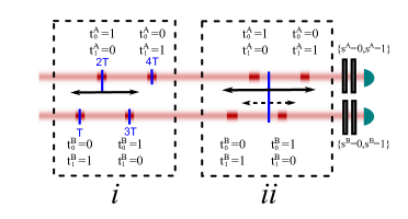
Figure 1: A diagram illustrating the coincidence-time loophole. Here $t^{A}_{z}=1$ $(t^{A}_{z}=0)$ corresponds to a detection event (no detection event) when Alice chooses measurement setting $s^{A}=z$, and similarly for Bob. In diagram i, a coincidence window (black arrow) is selected based on Alice’s detection event. A hacker can exploit this loophole by staggering pulses in time as shown. In this case, if the radius (half width) of the coincidence window is between $T$ and $3T$, there are no $\{s^{A}=1,s^{B}=1\}$ coincidence counts, implying that $B_{CH}$ in Eq. 1 is greater than $0$, even for a classical source. In diagram ii, a well-defined trial is used, where the window is centered on a synchronization pulse (blue line); the loophole vanishes as there is no longer a way to address only the $\{s^{A}=1,s^{B}=1\}$ coincidence term. If a large coincidence window (solid arrow) is used, then every measurement setting has a coincident event, resulting in $B_{CH}=0$. If a short trial window (dashed arrow) is used, then there are only coincident and single events at settings $\{s^{A}=0,s^{B}=0\}$, giving a Bell value of $B_{CH}=-1$.

II Analysis Description

A high-level explanation of the coincidence-time loophole is that the non-local method for inferring trials invalidates the assumptions underlying the Bell inequalities. The solution is to ensure that each party knows in advance the time and duration of a trial and relates recorded data accordingly. Moreover, if the settings are held fixed over multiple trials, it is necessary to make additional assumptions; for example, one can assume that the trials are independent and identical. To avoid making such additional assumptions, one should predefine trials such that they are associated with the time intervals between making random settings choices. (An alternative using party-dependent coincidence window sizes is described in Ref. Larsson2014 .) For the experiments analyzed here, this means that each party’s measurement outcome is their entire timetag sequence recorded between making settings choices, rather than a single detection or non-detection. Thus, the complete results from a trial consist of each party’s settings choice and the timetag sequences they measured before the next setting was applied. Note that in the absence of large separations between $A$ and $B$, this may make it difficult to ensure locality by space-like separation of relevant events. In two of the experiments below we can exclude all local realistic probabilistic models, but in principle, a hacker could have exploited the ability to communicate settings between $A$ and $B$ before the end of a trial to effect arbitrary, non-local-realistic probability distributions.

Generalizing the notation introduced above, we denote the timetag-sequence measurement outcomes of the two parties by $t^{A}_{s^{A}}$ and $t^{B}_{s^{B}}$, where $t^{A}_{s^{A}}$ denotes $A$’s outcome with the subscript $s^{A}$ indicating the setting used, and similarly for $B$. Since the settings choices are under experimenter control, their probability distribution is known. For the Bell tests considered here, each of the four setting-choice combinations has probability $1/4$.

To review the principles of the analysis method in KnillTBP , consider first a general local-realism test. The method begins by constructing a Bell function $B$ of trial results such that a Bell inequality in the form

$$\langle B(t^{A}_{s^{A}},t^{B}_{s^{B}},s^{A},s^{B})\rangle_{\mathrm{LR}}\leq 0$$ (2)

holds for all local realistic models. Here, $\langle\ldots\rangle_{\mathrm{LR}}$ denotes the expectation with respect to a local realistic probability distribution, where the settings distribution is fixed as above. Given such a Bell function, a violation can be demonstrated in an experiment by showing a statistically significant positive value for an empirical estimate $\hat{B}$ of $\bar{B}=\langle B(t^{A}_{s^{A}},t^{B}_{s^{B}},s_{A},s_{B})\rangle_{\mathrm{EX}}$, where $\langle\ldots\rangle_{\mathrm{EX}}$ denotes the expectation with respect to the experimental probability distribution. The traditional method for evaluating significance is via the sample standard error of $\hat{B}$. This can be used to assign approximate confidence intervals for $\bar{B}$ but cannot quantify the extremely high significance of the evidence against local realism that we seek. To quantify the significance, it is desirable to determine $p$-value bounds in the framework of statistical hypothesis testing. Ref. Zhang2013 shows how to systematically use lower-bounded Bell functions to obtain such bounds from the trial results.

A general strategy for constructing Bell functions that can be used for conservative estimates of $\bar{B}$ and $p$-value bounds is given in Ref. KnillTBP . Here, “conservative” means that the estimates and bounds are statistically valid with no approximations or extra assumptions on distributions other than the standard ones, namely that the settings probabilities are known and that local realistic distributions are mixtures of outcomes determined by the local settings. The fundamental principle is to start with settings-dependent “distance” functions $l_{s^{A},s^{B}}(t^{A},t^{B})$ on the measurement outcome pairs; such functions are required to satisfy a generalized, twice-iterated triangle inequality

$$l_{1,1}(t_{1}^{A},t_{1}^{B})\leq l_{1,0}(t_{1}^{A},t_{0}^{B})+l_{0,0}(t_{0}^{B},t_{0}^{A})+l_{0,1}(t_{0}^{A},t_{1}^{B}).$$ (3)

(If $l$ is non-negative and independent of the settings, then this is the conventional twice-iterated triangle inequality. Here we use the term “distance function” to refer to any function family $l$ satisfying Eq. 3.) Since local realistic models are given by probability distributions over deterministic models where a party’s setting determines the party’s measurement outcome, a Bell function can be constructed from $l$ according to

$$B(t^{A}_{s^{A}},t^{B}_{s^{B}},s_{A},s_{B})=\left\{\begin{array}[]{ll}l_{1,1}(t^{A}_{1},t^{B}_{1})&\textrm{if $s_{A}=1$, $s_{B}=1$},\\ -l_{1,0}(t^{A}_{1},t^{B}_{0})&\textrm{if $s_{A}=1$, $s_{B}=0$},\\ -l_{0,0}(t^{B}_{0},t^{A}_{0})&\textrm{if $s_{A}=0$, $s_{B}=0$},\\ -l_{0,1}(t^{A}_{0},t^{B}_{1})&\textrm{if $s_{A}=0$, $s_{B}=1$}.\end{array}\right.$$ (4)

The use of distance functions to obtain Bell inequalities was introduced by Schumacher in Ref. schumacher:qc1991a .

For timetag sequence outcomes associated with experiments that are intended to violate a CH-type inequality, Ref. KnillTBP shows that one can define distance functions according to a minimum cost of converting the first timetag sequence into the second by shifting and/or deleting timetags. A feature of the technique is that in the limit where the average time between detections is large compared to the time-jitter (the uncertainty in the time of the detection), the distance function can be made to match the value of any CH-type Bell function. One issue is that the costs defining the distance function are parametrized, and we wish to choose these parameters optimally given the characteristics of the experiment. However, to avoid biases and remain conservative, it is necessary to choose the parameters beforehand, independent of the data to be analyzed. That is, contrary to what is often done in experiments, no part of the “final data” can be used to find analysis parameters, such as delays. Otherwise the validity of confidence intervals or $p$-values is lost. The parameters can instead be determined by setting aside a fraction of the trials from the beginning of the experiment. This “training data set” is used for optimizing analysis parameters. The remainder of the trials constitute the analysis data set and should only be analyzed once the parameters have been chosen. In the applications below, the training set serves to determine two Bell functions. The first is designed to maximize a CH-like violation and can be compared to traditional (that is, non-distance-based) measures of violation. For reporting these violations, we modify the conventional method so that the violation reported is meaningful without assuming that the trials are independent, as explained in App. C. The second Bell function is a systematically “truncated” version of the first; the truncation method is general and can be applied to any distance-based Bell function KnillTBP . The second Bell function is bounded, so we can apply the techniques from Ref. Zhang2013 to obtain a $p$-value (upper) bound. As these $p$-value bounds are extremely small, we give their negative logarithm base $2$, called the $\log_{2}$-$p$-value (lower) bound. See Sect. IV for the interpretation of $p$-values and their comparison to Gaussian tails.

Because all the experiments discussed below were performed before the statistical techniques were fully developed, their analysis was retrospective and in this sense deviated from the ideal protocol; the deviations are discussed in App. B.

III Experimental realization of the coincidence-time loophole

We realized the coincidence-time loophole experimentally by combining two attenuated lasers on a beam splitter for both Alice and Bob (Fig. 2). For Alice, one laser is polarized orthogonal to the polarizer setting for measurement setting $s^{A}=0$, while the other laser is polarized orthogonal to the polarizer setting for $s^{A}=1$, and similarly for Bob. This allows the source to address the measurement settings independently (i.e., when we send a laser pulse polarized along $(s^{A}=1)^{\perp}$, we should only receive detection events for measurement setting $s^{A}=0$). We then attenuate the sources to a mean photon number per pulse of around $10$. The relatively high mean photon number offsets the loss in the measurement and detection process, but is still small enough to minimize the effect of crosstalk in the polarizer (there is a small chance that the polarization state to be blocked is still transmitted through the polarizer). We then pulse the lasers as shown in Fig. 1, with adjacent pulses separated by $T=1\,\mathrm{\mu s}$. If we determine the number of coincidence events by checking if Bob had a detection event within a window (e.g., $2\,\mathrm{\mu s}$) around Alice’s detection events, then we observe Bell inequality violations up to $B_{CH}=0.49$ (with the normalization discussed earlier), where Alice and Bob use the optimal settings for an ideal maximally entangled state as specified in the caption of Fig. 1. A plot of the data analyzed in this way is displayed in Fig. 3. We see a “violation” of over $2700$-$\sigma$ (assuming Gaussian statistics). By altering the two laser polarizations and increasing the mean photon number to offset any additional losses, we have been able to exploit this loophole for a wide range of measurement settings, see App. A.1. In addition, the degree of violation can be altered by changing the laser polarization. As a final note, while the plot in Fig. 3 has a well-defined structure, it is possible to broaden the observed “violation range” by probabilistically switching between local hidden-variable models with different pulse spacings; therefore, one cannot simply look at a plot of the Bell violation versus coincidence window size to determine if the coincidence-time loophole is being exploited.

In contrast, if we use a predefined coincidence window centered on a predefined time rather than one centered on a detection (see App. A.2 for details), we do not see a statistically significant Bell violation, as shown in Fig. 3. Furthermore, when we use the distance-based analysis from Ref. KnillTBP , the results correctly do not indicate that the system is behaving contrary to local realism. Initially, in the training set, where delays are determined to offset electronic latencies, the delays on apparent coincidences were found to depend highly on the measurement settings, due to the scheme for exploiting the coincidence loophole. From the other experiments using the same setup, the latencies are known to be small, so for demonstration purposes we ignored this observation and did not offset for electronic latencies. The distance-based Bell function (Eq. 4) is then significantly negative, showing no evidence against local realism according to this analysis.

While the data set in this case is contrived to be clearly determined by a local hidden-variable model, in real experiments the issues are far more subtle. For example, avalanche photo-diodes can have a count-rate-dependent latency, and since each measurement setting can have different detection rates (for example, in Ref. Christensen2013 , the count rates differed by a factor of 3), it is critical that the analysis is not susceptible to these minor latency shifts. To show that these issues are relevant, Ref. KnillTBP presents a coincidence-loophole-exploiting scheme whose statistics closely match those of a standard photon-pair source.

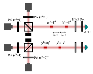
Figure 2: A diagram of our experimental setup to produce the local hidden-variable model described in Fig. 1. On Alice’s side, we electrically pulse two lasers with a pulse width of $100\,\mathrm{ns}$; these pulses then pass through polarizers aligned orthogonally to her two measurement settings (Pol $(s^{A}=0)^{\perp}$ and Pol $(s^{A}=1)^{\perp}$). That is, we emit pulses that will not pass through one of the two measurement settings, ensuring only one of the measurement settings will detect our optical pulse. The laser pulse that passes through the $(s^{A}=0)^{\perp}$ polarizer is emitted $2\,\mathrm{\mu s}$ before the $(s^{A}=1)^{\perp}$ laser pulse. We attenuate the lasers enough so that after they are combined on a beam splitter, each pulse has a mean photon number of approximately $10$, to offset any system loss while minimizing the noise due to crosstalk in the polarizers. Similarly on Bob’s side, we combine two attenuated lasers on a beam splitter. Here, the $(s^{B}=1)^{\perp}$ pulse is emitted $2\,\mathrm{\mu s}$ before the $(s^{B}=0)^{\perp}$ pulse. Both are offset from Alice’s photon pulses by $1\,\mathrm{\mu s}$. The basis choice for the polarization analysis is implemented with a half-wave plate (HWP) and polarizer (Pol), where the settings are $-11.25^{o}$ for $s^{A}=0$, $33.75^{o}$ for $s^{A}=1$, $11.25^{o}$ for $s^{B}=0$, and $-33.75^{o}$ for $s^{B}=1$ (corresponding to the optimal CH-Bell-inequality-violating settings of a perfect maximally entangled state). The photons are then detected by an avalanche photo-diode (APD), with an efficiency lower than $66\,\mathrm{\%}$, the outputs of which are recorded using a time-to-digital converter. The results of analyzing the data both with a coincidence window determined by Alice’s detection event, as well as a predefined coincidence window, is displayed in Fig. 3.

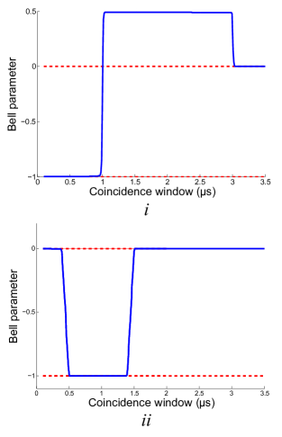
Figure 3: Two plots of the measured Bell parameter, $B_{CH}$ (Eq. 1) (solid blue line), as a function of the coincidence window radius for our experiment using a classical source to produce the local hidden-variable model shown in Fig. 1. When the data set is analyzed with a coincidence window determined by a detection event (diagram i), the coincidence-time loophole can be exploited to produce a Bell violation (values greater than 0). We separated each pulse by $1\,\mathrm{\mu s}$, so with this model we see $B_{CH}>0$ for any coincidence window radius between $1\,\mathrm{\mu s}$ and $3\,\mathrm{\mu s}$. For coincidence windows less than $1\,\mathrm{\mu s}$, we do not have any coincidence counts, but we still have single counts, resulting in a negative Bell parameter of $B_{CH}\geq-1$. While this value depends on the chosen normalization, the minimal inferred value of $r_{p}$ is at $r_{p}=2r_{h}$, resulting in the most negative Bell parameter of $-1$. With window sizes larger than $3\,\mathrm{\mu s}$, we assign coincident and single events to nearly every detection event, resulting in a Bell parameter of $0$. In contrast, analysis with a fixed predefined coincidence window (diagram ii), or using the technique described in the text, never produces a violation for any window size. When the data set is analyzed with a predefined coincidence window, the Bell parameter remains between -1 and 0, and therefore does not show a violation of local realism. The results match well the predictions given the structure of the classical source as explained in App. A.2. The positions of the transitions are due to the location of the predefined coincidence window relative to the pulse set. The transitions between $0$ and $-1$ are not sharp because of the slow desynchronization between the fixed windows and the actual source pulse rate. That is, the window slowly drifts such that it is not always centered on the pulse set. For more details, see App. A.2.

IV Experiments with violation

The example above shows the use of the distance-based analysis technique to “catch” an invalid violation of a Bell inequality with a purely classical source. The following two examples demonstrate the strength of this analysis on data with actual quantum correlations.

First, we consider the data collected and analyzed in Ref. Christensen2013 , where the experiment had a high enough system efficiency and low enough noise to be able to violate a CH Bell inequality. The data set was taken with an external clock synchronized to a laser pulse. A predefined coincidence window of $2.4\,\mathrm{\mu s}$ was centered around the laser synchronization pulse, from which a trial could be well defined, avoiding the coincidence-time loophole discussed above. The data set was collected by changing the measurement settings randomly every second, collecting for $4450$ different measurement setting choices. For the analysis in Ref. Christensen2013 , the data set was partitioned into $50$ different Bell tests. The uncertainty was calculated from the distribution of the $50$ different Bell parameters using the sample standard error. The reported value from this approach was $B_{CH}=5.4\times 10^{-5}\pm 7.0\times 10^{-6}$, a $7.7$-$\sigma$ violation, where the conventional interpretation of the large violation assumes Gaussian statistics. In contrast, here we analyze the same data set with the distance-based method without making distributional assumptions or approximations. Additionally, whereas the previous analysis required each pulsed trial to be independent and identical to allow for the settings being fixed, the new analysis, detailed in App. B, treats each $1\,\mathrm{s}$ period with fixed settings as one trial and therefore does not require this assumption. We find a $\log_{2}$-$p$-value bound of $33$, which means that for every local realistic model, the probability that this analysis reports a $\log_{2}$-$p$-value above $33$ is less than $2^{-33}=1.16\times 10^{-10}$, a very unlikely event. While this result is equivalent to a $6.3$-$\sigma$ violation for Gaussian statistics (we give the Gaussian-equivalent violation only for comparison; it is computed from the $p$-value bound of $2^{-33}$ by solving $\int_{x}^{\infty}e^{-x^{2}/2}/\sqrt{2\pi}=2^{-33}$ for $x$), slightly lower than the $7.7$-$\sigma$ violation reported in Ref. Christensen2013 , it does not assume Gaussian statistics. Thus, we see that with minimal degradation of the evidence for Bell-inequality violation, we have reduced the required assumptions on the system: the trials do not need to be independent and identical and the distributions are not approximated by Gaussians. If the system is being hacked, lack of independence and Gaussianity are even more pronounced.

Finally, we consider a different data set taken on the same high-efficiency system, but with neither pulsing the laser nor having an external clock. To analyze the data conventionally, we partition time into segments independent of the data (that is, we impose a fixed coincidence window). Since we are not determining the coincidence window based on the data, it is not susceptible to the coincidence-time loophole (see Fig. 1ii). However, because we are introducing a coincidence window that is not related to the arrival time of photons, due to the detector time-jitter, we are effectively introducing loss into the system. That is, if the window is small compared to the time-jitter, then it is possible that Alice and Bob’s detection events from a single pair of photons are nevertheless registered in different time segments, resulting in two single counts without a coincidence count. In the opposite limit, the window becomes too large, which reduces the Bell parameter due to the high likelihood of counting uncorrelated photon pairs as coincidences. The result of analyzing the data in this way is displayed in Fig. 4. While the source quality is sufficient for a Bell test (that is, it has high heralding efficiency and high entanglement quality), the effective loss introduced by this conventional analysis is too much for us to adequately extract the quantum correlations. If we instead analyze the data using the distance-based approach discussed here, we find a violation with a $\log_{2}$-$p$-value bound of $269$, the equivalent of a $19$-$\sigma$ violation (see App. B for more details). In addition to revealing a violation where conventional analysis would not produce one, the confidence in the violation is actually significantly larger than that with the pulsed source presented in Ref. Christensen2013 . This is because we can utilize a system that is “on” more often than a pulsed source (which by definition has no data collection between pulses), thereby resulting in substantially more data.

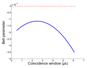
Figure 4: A plot of the CH-Bell parameter from a non-pulsed experiment, analyzed using different predefined coincidence windows. While the system is capable of a detection loophole-free violation as verified in Ref. Christensen2013 , the inefficiencies of a conventional analysis with predefined coincidence windows are unable to produce a non-classical result: for small window sizes, the analysis introduces loss because of the timing uncertainty (time-jitter) of the detectors, causing the mis-assignment of some detection events as non-coincidence counts; large windows increase the system noise, to which the CH Bell inequality is very sensitive, again resulting in a reduced Bell parameter. Here we show the Bell parameter for many different coincidence windows, the blue solid line is a fit to all of the data points (the points are spaced by $10\,\mathrm{ns}$), each of which lie within the thickness of the line. With conventional analysis, we do not observe a Bell violation (above the red dashed line) for any coincidence window. With the new analysis discussed in KnillTBP , we observe a violation with a $\log_{2}$-$p$-value bound of $269$.

V Discussion

As shown in the above examples, the distance-based analysis of Ref. KnillTBP is able to improve the statistical significance of a Bell inequality violation, as well as reduce the required assumptions compared to a standard analysis. While the analysis uses distance functions as a measure of the violation, it has important features common to any conservative analysis of Bell inequality data. First, to estimate the significance of the violation, it is important to use $p$-value bounds instead of standard deviations. The latter are unreliable for the high significance of typical Bell inequality violations. Second, to prevent overestimating the statistical significance of the Bell inequality violation, delays, coincidence windows and other such analysis parameters should be determined from a training data set (that is then discarded) rather than the data to be analyzed. Otherwise, if the final data set is used to determine these parameters, the reported violation may be biased by statistical fluctuation rather than reflect a fair estimate. Finally, all Bell tests should have predefined trials to avoid opening up additional loopholes (e.g., the coincidence-time loophole). The predefined trials may be based on a timetag sequence according to the chosen settings as presented here, specific laser pulses detected on a photodiode as presented in Ref. Christensen2013 , or the detection of heralding photons as in the ion experiments of Ref. Pironio2010 .

Appendix A Additional Experimental Details

This section further discusses our classical source that exploits the coincidence time loophole. The first subsection explains how the source can be tuned to match Alice and Bob’s expectations (i.e., to give violations consistent with quantum mechanics). In the second subsection we use a predefined coincidence window to analyze the data from the classical source and find no violation of local realism.

A.1 Controlling Violation Size

In an actual attempt of a Bell test, Alice and Bob would likely suspect the presence of a hacker if their estimated CH-Bell parameter is beyond the quantum mechanical limit of $(\sqrt{2}-1)/2$. Even more so, if Alice and Bob know that they have low system efficiencies, then the value they expect is well below $(\sqrt{2}-1)/2$. In particular, with low efficiency, Alice and Bob design their system to use states of the form $\cos{\theta}|HH\rangle+\sin{\theta}|VV\rangle$ (see Ref. eberhard:qc1993a ; Giustina2013 ; Christensen2013 ) to maximize the measured violation. Consequently, a hacker would want Alice and Bob to believe that they prepared a less entangled state (states with $\theta$ farther from $\pi/4$). If Alice and Bob estimate $\theta$ for their state, they obtain a maximum Bell parameter they expect. Ideally, the hacker controls the measured Bell parameter to match Alice and Bob’s expectation and avoid suspicion. In our case, with the source depicted in Fig. 2, we can tune the input polarizers (and adjust the laser diode brightness to compensate the increased loss) to create nearly any value of the Bell parameter. The results of a few measurements using this technique are displayed in Fig. 5.

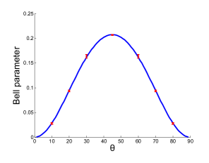
Figure 5: A plot of a few measured data points from our classical source when analyzed incorrectly (susceptible to the coincidence-time loophole discussed in Sect. I). The blue curve is the predicted quantum mechanical maximum given the state $\cos{\theta}|HH\rangle+\sin{\theta}|VV\rangle$. Here, we assumed Alice and Bob have a target $\theta$ and use the optimal measurement settings for the input state. We then adjusted the input polarizer angle to match the quantum mechanically allowed maximum Bell parameter, given Alice and Bob’s measurement settings. The results of a few measurements are displayed as the red data points, which are indistinguishable from the quantum mechanical expectation.

A.2 Predefined Window Analysis

To use a predefined window to analyze the data exploiting the coincidence-time loophole, we first add in a synchronization signal at the rate equal to the rate that the source emits a set of pulses, 100 kHz in our case. As there was no actual synchronization signal when the data set was taken, we implement this signal in post-processing. For comparison with Fig. 1ii, where the predefined coincidence window is in the center of the pulse set, we placed the first synchronization signal in the center as determined by the first two detection events in the data set. We then create a periodic signal by spacing each synchronization signal by 10 $\mu$s ($=1/100$ kHz). To compensate for the relative temporal drift between the function generator and the timetagging electronics, we reset the synchronization signal every 500 detection events to be re-centered in the pulse set. If the separation between adjacent pulses is 1 $\mu$s (see Fig. 2), then we would expect a Bell parameter close to 0 for windows less than 0.5 $\mu$s, since there will be neither single nor coincident events (other than occasional dark counts, no event will fall within the predefined window). For windows between $0.5\,\mathrm{\mu s}$ and $1.5\,\mathrm{\mu s}$ we would expect a Bell parameter close to $-1$, since we see events primarily from $\{s^{A}=0,s^{B}=0\}$. That is, $p_{AB}(t^{A}_{0}=1,t^{B}_{0}=1)=1$, $p_{A}(t^{A}_{0}=1)=1$, and $p_{B}(t^{B}_{0}=1)=1$ in Eq. 1, while all other terms are 0. Finally, for predefined window sizes larger than 1.5 $\mu$s, all terms in Eq. 1 are equal to $1$, leading to a Bell parameter of 0. The results of analyzing the classical data with a predefined coincidence window of variable width are displayed in Fig. 3.

Appendix B Discussion of Analyses

Here we describe in detail the distance-based analyses of the data from the three experiments discussed in the paper. The results reported are from final analyses that adhered to the protocol of inferring parameters from the training set and applying them adaptively to the analysis set. However, the final analyses were not strictly blind; the data set was available for some time while our analysis methods were being developed and there were multiple early analysis attempts involving various techniques. Features of the data discovered in these attempts required changes in preprocessing and strategy. These changes are described below as needed.

Each data set was analyzed by two or three methods for comparison purposes. The simplest method is a conventional analysis based on coincidence counting. The results of this method are susceptible to the coincidence loophole and require strong assumptions on the source and its statistics. The second method involves our distance-based Bell-function analysis applied to trials consisting of all the data acquired while the settings were held fixed. The third computes “certificates” of violation (given as $\log_{2}(p)$-values) using the prediction-based-ratio (PBR) protocol zhang_y:qc2011a ; Zhang2013 with truncated versions of the distance-based Bell functions. We discuss the analysis of the three experiments in reverse order, which is also the order in which the data sets were received and analyzed.

B.1 Continuously Emitting Quantum Source

The data set for this experiment consists of $3953$ trials with randomly chosen settings. The measurement outcomes consist of a sequence of timetags for each party, where each timetag records a detection event. The average numbers of recorded detections per trial are approximately $1400$ on setting $1$ and $4900$ on setting $2$ for both parties. Each trial’s results are stored in one file. The files for eight trials were corrupted and therefore discarded, leaving $3945$ trials. The timetag sequences were preprocessed in two steps. The preprocessing parameters were determined at an early stage of analysis with a set consisting of $97\times 4$ randomly chosen trials with $97$ at each settings choice. (The final analysis was performed in the order in which the experiment was performed with the initial trials used for training–see below. The preprocessing parameters suggested by the training set for the final analysis were the same up to statistical fluctuations, so we did not change them for the final analysis.) The first preprocessing step compensated for transient artifacts near the beginning and end of the timetag sequences. We therefore used only timetags from the middle portion of the sequence determined as follows: The sequence durations are approximately $1\,\mathrm{s}$. For each trial, we first determined the earliest recorded time $t_{0}$ in both parties’ sequences and set $t_{0}^{\prime}$ to be the second multiple of $10^{8}$ past $t_{0}$ (in the time units used for the timetags, $156.25\,\mathrm{ps}$) Thus $t_{0}^{\prime}=(\lfloor t_{0}/10^{8}\rfloor+2)10^{8}$. We then used only timetags with recorded times $t$ satisfying $t_{0}^{\prime}\leq t\leq t_{0}^{\prime}+6\times 10^{9}$. We remark that this preprocessing step is non-local, which is in general undesirable. We are not aware of any way in which a local realistic (LR) source could exploit this, though the possibility exists. The second preprocessing step corrected a systematic timing offset between the recorded times for the two parties. The offset was applied to all timetag sequences of party $A$ and involved shifting the timetags by $-685$ time units (i.e., $107\,\mathrm{ns}$). For comparison, the time-jitter determined as the typical distance between apparent coincidences is of the same order.

All analysis attempts used the preprocessing of the previous paragraph. We describe the final analysis first and then discuss how we arrived at the final analysis. For the conventional analysis, we used the first $197$ trials to determine the optimal coincidence window. We then computed the number of coincidences for each trial. The coincidences were determined as described in KnillTBP rather than with the simple Alice-centered windows used in the main text. We then computed the estimated total violation as described in App. C according to the Bell-inequality used for the original analysis of the pulsed quantum source in Ref. Christensen2013 . The total violation according to this analysis is $5.14(10)\times 10^{4}$, corresponding to a nominal signal-to-noise ratio (SNR) of $59.7$. The latter is the ratio of the total violation to the estimated uncertainty; see App. C.

The distance-based analysis was performed adaptively. An adaptive procedure was required because the parameters of the distance-based Bell function used are sensitive to the apparent drifts in count-rates over time. Starting at the $201$st trial and then every $400$ trials, we re-optimized the Bell function parameters on the previous $800$ trials. (Before the $801$st trial we used all the trials already processed, including the first $200$.) The Bell function was then computed for each of the next $400$ trials, before re-optimizing the parameters. We then estimated the total violation as described in App. C. The total violation according to the distance-based analysis is $2.52(10)\times 10^{4}$, corresponding to a nominal SNR of $24.5$.

The Bell-function values from the distance-based analysis were then used in an adaptive version of the PBR analysis. This required adaptively computing the parameters for Bell-function truncations and the mixtures used in constructing the test factor according to the protocol in Ref. KnillTBP . This proceeded similarly to the distance-based analysis, except that the parameters were updated every $10$ trials and optimized on the last $400$ (or less) trials. We chose the more frequent update because there is little computational cost in doing so and the truncation and mixture parameters are sensitive to small drifts in the conditional means of the Bell function. The $\log_{2}(p)$-value bound obtained is $269$, equivalent to a one-sided Gaussian SNR of $19$.

The final analysis was performed after two previous analyses. The first analysis involved partitioning the trials into randomly chosen sets of four matched trials, one at each of the settings choices. The version of the distance-based analysis available at the time yielded a significantly smaller total violation than the final analysis. The PBR analysis at the time was faulty, but suggested a significantly higher $\log_{2}(p)$-value bound than revealed by the final analysis. Because the randomization strategy used in this analysis is not acceptable for certification purposes, a second analysis was performed after the analysis procedures were updated. During this analysis, we discovered that the count-rate variations in time significantly affect the $\log_{2}(p)$-value bounds, requiring that the analysis be performed adaptively. A choice for adaptation parameters was made after investigating the timescale of the variations. The estimated total violation found was the same within error bars as the one for the final analysis. The third and final analysis was required because we discovered an error in our original method for Bell function truncation in the PBR analysis resulting in an overly optimistic $\log_{2}(p)$-value. The adaptation parameters were chosen for the final analysis based on our experience in the second round of analysis. Because of this history, a moderate bias in the estimated total violation and in the $\log_{2}(p)$-value bounds is expected.

B.2 Pulsed Quantum Source

The data set for this experiment consists of $4450$ trials. The settings for each trial were chosen randomly. Each party’s measurement outcome consists of a sequence of time-tagged detections. The source was pulsed with the pulses synchronized with a clock whose “ticks” were also recorded for each trial. There are approximately $12500$ pulses per trial before preprocessing. The original analysis of the data reported in Ref. Christensen2013 analyzed each pulse as a trial. To consider the results of this analysis as evidence against LR requires an assumption such as that each pulse is independent and identical. Defining trials so that they contain all the measurements that occur while the settings are fixed avoids making this assumption.

The sequences of timetags from each trial were preprocessed as follows: We first corrected for the time-offset of $A$ as we did for the data from the continuously emitting source. We then removed detections outside narrow windows containing each pulse. The windows were determined relative to the recorded clock ticks and have a width of $16000$ time units. The pulses are separated by about $256000$ time units. We dropped the first $200$ pulses and saved the $12200$ subsequent pulses, dropping the rest. To correct for intermittent interference causing excess detections, we “blanked out” (removed detections in) pulses where there was an excess number (three or more) of detections outside pulse windows in the period spanning three pulses before and after. Note that the preprocessing is local in the sense that the parties can in principle perform it without communicating, given that they have synchronized clocks.

As in the case of the continuously emitting source, there were several analysis attempts. In the first attempt, the order of the trials was randomized and we only confirmed that the violation based on distance-based analysis was consistent with the results reported in Ref. Christensen2013 . The PBR analysis was not performed at this time. Later analyses were performed in parallel with the analysis of the continuously emitting source, with the final analysis correcting the same problem with our original implementation of Bell-function truncation.

For the final analysis, we did not perform a version of the conventional coincidence analysis as the pulsed nature of the source made this unnecessary. Applying the distance-based analysis using the distance-based Bell functions of Ref. KnillTBP failed to show a violation; we attribute this to the presence of an excess of multiple detections during pulses and the sensitivity of the analysis to detection-rate changes. (We attribute most multiple detections to local detection artifacts, such as detector after-pulsing, rather than photons. These local effects confuse the distance-based analysis by adding non-violating LR signals.) We therefore used a simpler Bell-function with no parameters. This Bell-function is obtained by adding the Bell-function derived from the Bell inequality used in Ref. Christensen2013 over the detections for each pulse. For this purpose, multiple detections in a pulse are counted as one. This is an instance of a general strategy for pulsed sources where the settings are not changed for every pulse. Consider a Bell function $B$ for the detections from one pulse satisfying the Bell inequality $\langle B(T,S)\rangle_{\textrm{LR}}\leq 0$, where $T$ is the detection pattern and $S$ the measurement settings. If we have a sequence of pulses at fixed measurement settings $S$ with detection patterns $T_{i}$, we can define a Bell function $B^{\prime}(\mathbf{T},S)=\sum_{i}B(T_{i},S)$, where $\mathbf{T}$ is the sequence of detection patterns $T_{i}$. The Bell inequality $\langle B^{\prime}(\mathbf{T},S)\rangle_{\textrm{LR}}\leq 0$ is also satisfied by $B^{\prime}$. To avoid assuming that trials are independent and identically distributed (i.i.d.), one can analyze the violation of $B^{\prime}$ instead of $B$. This change of view enables the PBR analysis: As noted in Ref. KnillTBP , all Bell functions for two parties and two settings can be derived from a set of distance-like functions satisfying an iterated triangle inequality. This makes it possible to apply the PBR analysis as we have done here. Although the parameters of the Bell-function require no training, the total violation was computed using the procedure of App. C with an initial set of $200$ trials set aside for initializing the predictions. In each step, the predictions in the procedure were updated using the previous $200$ trials to account for experimental drift. The distance-based analysis found a total violation of $1.41(18)\times 10^{3}$, corresponding to a nominal SNR of $7.8$.

For the PBR analysis, we computed the necessary truncation and mixture parameters adaptively based on the Bell function values obtained in the Bell function analysis. The first $400$ trials were reserved for training. Starting with the $401$st trial, we updated the parameters every $200$ trials based on the previous $1600$ trials (or less, initially). We found a $\log_{2}(p)$-value bound of $33$, equivalent to a one-sided Gaussian SNR of $6.3$.

B.3 Classical Source

The experiment on the classical source consisted of $9$ groups of four trials at each of the four settings choices. The settings were not chosen randomly. Thus the interpretation of an apparent violation requires i.i.d. assumptions. Of course, the source was designed to be LR, so no real violation can be observed. The data from this experiment was analyzed just once, after the distance-based analysis matured. Each trial has approximately $97000$ detections for each party independent of the settings. The first group was set aside for training. A first step in all our analyses was to determine systematic timing offsets and an estimate of the time-jitter, both were done by checking timetag differences on apparent coincidences. For this source, the timetag differences immediately revealed that there was an “unexpected” pattern in the detections. That is, since there was no attempt at hiding that the source was exploiting the coincidence-time loophole, the resulting characteristic detection delays are obvious. (Ref. KnillTBP demonstrates a simulated source that can successfully hide these detection patterns.)

For the purpose of demonstrating that a standard coincidence analysis (windows determined by Alice’s detections) is deceived by this source, we optimized the coincidence window as usual on the training set and applied the coincidence analysis to the rest. The total violation found was $6.6488(24)\times 10^{5}$ for a large nominal SNR of $2781$. We optimized the Bell function for the distance-based analysis but were unable to detect a violation. In fact, the estimated total Bell function was significantly negative. We cannot exclude the possibility that a better choice of parameters for the timetag Bell function exists, though we know on theoretical grounds that a violation should not be observable according to the distance-based analysis. Given the absence of violation, the PBR analysis is guaranteed to use trivial test factors giving a $\log_{2}(p)$-value bound of $0$.

Appendix C Conservative Estimates of Bell-Violation

For each experiment, the timetag Bell function $B$ used has expectations that are related to the violation of a CH-type inequality by multiplying the latter by the expected number of photon pairs. In the limit of low time-jitter compared to the mean photon-pair inter-arrival time, the expectations according to $B$ and that expected from the CH-type inequality converge. It is therefore worthwhile to estimate the expected value of the Bell function for comparison purposes. In principle, for each trial, the expectation of $B$ is an experimental observable that, if greater than zero, witnesses violation of the Bell inequality associated with $B$. If the trials are i.i.d., the expectation can be estimated empirically using conventional methods. For tests of LR, this is usually done by estimating the settings-conditional expectations of $B$, which are then added. The uncertainty is obtained accordingly. When the trials are not necessarily independent or identical, there may be no single expectation of $B$ to estimate, so the conventional method cannot be used. Here we give an alternative that produces meaningful results in the general case. It statistically agrees with the conventional method when the trials are i.i.d.: While the estimated uncertainties obtained are slightly larger on average, they differ by an amount that is comparable to the expected statistical fluctuations in the estimate.

We emphasize that the purpose of these methods is to obtain an estimate of a physical quantity and the associated uncertainty. They do not yield certificates against LR (see Zhang2013 for a discussion). While we obtain uncertainties that are appropriate for dependent trials whose expectations change in time under normal experimental conditions, a sufficiently determined adversary can still ensure that our uncertainties are overly optimistic.

Here is the procedure for our method. A mathematical discussion follows the procedure.

• • Initialize the running value of the estimated total Bell violation by setting $\hat{b}_{[0]}=0$.

  • Initialize the running value of the estimated variance $\hat{u}_{[0]}=0$

• For each trial result $d_{i}$, $1\leq i\leq N$ in order, do the following

  • Before considering $d_{i}$:

    • Predict the settings-conditional expected Bell-function values $\langle B(D_{i})|S_{i}=s\rangle$ at the next trial as $b_{\mathrm{pred},i}(s)$. This prediction can be based on any information available before the $i$th trial occurred, including calibrations, theory and previous trial results. Here, $S_{i}=(S^{A}_{i},S^{B}_{i})$ are the joint settings random variables and $D_{i}$ are the random variables whose outcome values are the $d_{i}$.

    • Determine the predicted average Bell function violation $\bar{b}_{\mathrm{pred},i}=\sum_{s}b_{\mathrm{pred},i}(s)p_{s}$, where $p_{s}$ is the probability of settings choice $s$. Note that $\langle b_{\mathrm{pred},i}(S)\rangle=\bar{b}_{\mathrm{pred},i}$ is known exactly before the $i$th trial.

  • Now consider $d_{i}$:

    • Compute $\hat{b}_{[i]}=\hat{b}_{[i-1]}+B(d_{i})-(b_{\mathrm{pred},i}(s_{i})-\bar{b}_{\mathrm{pred},i})$.

    • Compute $\hat{u}_{[i]}=\hat{u}_{[i-1]}+(B(d_{i})-b_{\mathrm{pred},i}(s_{i}))^{2}$.

• Report the estimated total Bell violation as $\hat{b}_{[N]}$ with an approximate $68\,\%$ confidence interval of $\hat{b}_{[N]}\pm\sqrt{\hat{u}_{[N]}}$.

The simplest method for predicting the settings-conditional Bell-function expectations in step 2.a.1 of the procedure is to compute the sample means conditional on settings from the first $i-1$ trials and the training trials. This works well for stable experiments. For the data analyses in this paper, we used a segment of recent trials (including the training trials) instead. We formulated the procedure for a fixed Bell function, but the procedure also works if the Bell functions are chosen adaptively before each trial.

Consider a sequence of trials with each trial’s result given by $d_{i}$. We now adopt the usual conventions for random variables and their outcome values, where random variables are capitalized. Thus $D_{i}$ is the random variable for the result from the $i$th trial, and $d_{i}$ is its outcome value in a particular run of the experiment. The results consist of the measurement outcomes and settings. We let $T^{X}_{i}$ and $S^{X}_{i}$ be the respective random variables for the measurement outcome and setting of party $X$ in the $i$th trial. We let $D$ denote the sequence of random variables $D_{i}$. The random variables $D_{i}$ are not necessarily independent, but the distributions of the settings $S^{X}_{i}$ are jointly uniform and therefore independent of each other. We let $H_{i-1}$ be a random variable that captures the history of events preceding trial $i$, including events not captured by $D$ but that are relevant to the experiment. In particular, $H_{i-1}$ determines $D_{j}$ for $j<i$ and may include additional experimentally relevant information. The goal is to obtain an empirical estimate of the quantity

$$\bar{b}_{[N]}(h)=\sum_{i=1}^{N}\langle B(D_{i})|H_{i-1}=h_{i-1}\rangle,$$ (5)

and a confidence interval for this estimate. Here, $h_{i-1}$ is the actual value of the history random variable. Throughout, we assume that the relevant real-valued random variables have finite second moments. We interpret $\bar{b}_{[N]}(h)$ as the total Bell inequality violation actually present in the experiment, which we estimate with $\hat{b}_{[i]}$. We do not assume that the outcome value $h_{i-1}$ is known, just that it is well-defined for a given run of the experiment. Define $\bar{b}_{i}(h)=\bar{b}_{i}(h_{i-1})=\langle B(D_{i})|H_{i-1}=h_{i-1}\rangle$. This is the expected value of the Bell function for the upcoming $i$th trial, just before the trial is performed. We use the following conventions to refer to functions of random variables and the random variables defined by these functions: Except for the Bell function $B$, we use lower case annotated symbols for the functions. Applying a function to a random variable as in the expression $\bar{b}_{i}(H)$ defines a new random variable. To simplify the notation, we also refer to this random variable by its upper case variant, so that $\bar{B}_{i}=\bar{b}_{i}(H)$. (Here $H$ refers to the full history.) The outcome values of this random variable are then denoted by $\bar{b}_{i}=\bar{b}_{i}(h)$.

For i.i.d. trials, $\bar{b}_{i}(h)=\langle B(D_{i})\rangle$ and is independent of $i$ and $h$. The sum $\bar{b}_{[N]}(h)=\sum_{i=1}^{N}\bar{b}_{i}(h)$ can then be interpreted as the conventional total Bell inequality violation of the experiment, if it is positive. For the empirical estimate of $\bar{b}_{[N]}(h)$ we could compute $\sum_{i=1}^{N}B(d_{i})$, but instead we use the less-noisy estimate $\hat{b}_{[N]}$ from the procedure. The estimate is less noisy because we subtracted from $b(d_{i})$ the quantity $(b_{\mathrm{pred},i}(s_{i})-\bar{b}_{\mathrm{pred},i})$, whose mean is guaranteed to be zero but is expected to be positively correlated with the original estimate.

The first task is to show that $\hat{b}_{[N]}$ is an unbiased estimator of $\bar{b}_{[N]}(h)$ (that is $\langle\hat{B}_{[N]}\rangle=\langle\bar{b}_{[N]}(H)\rangle$). We use $E(A|B)$ to denote the conditional expectations of $A$ with respect to $B$ interpreted as a function of the random variable $B$. The notation $\langle\ldots\rangle$ is reserved for unconditional expectations and expectations conditional on specific outcome values. Since $E(\ldots|\ldots)$ denotes random variables, they may occur inside $\langle\ldots\rangle$. By expanding the definition, we have

$$\left\langle\hat{B}_{[N]}\right\rangle=\left\langle\sum_{i=i}^{N}B(D_{i})-(B_{\mathrm{pred},i}-\bar{B}_{\mathrm{pred},i})\right\rangle.$$ (6)

The expectation of $B_{\mathrm{pred},i}-\bar{B}_{\mathrm{pred},i}$ is $0$ by design, so

$$\left\langle\hat{B}_{[N]}\right\rangle = \sum_{i=i}^{N}\left\langle B(D_{i})\right\rangle$$ (7)

$$= \sum_{i=i}^{N}\left\langle E(B(D_{i})|H_{i-1})\right\rangle$$ (8)

$$= \sum_{i=i}^{N}\left\langle\bar{b}_{i}(H)\right\rangle$$ (9)

$$= \left\langle\bar{b}_{[N]}(H)\right\rangle,$$ (10)

where the identity $\left\langle B(D_{i})\right\rangle=\left\langle E(B(D_{i})|H_{i-1})\right\rangle$ follows from the rules for iterated conditional expectations. (This is a special case sometimes referred to as the “law of total expectations”.)

The second task is to determine an approximate $68\,\%$ confidence interval for $\bar{b}_{[N]}(h)$ around $\hat{b}_{[N]}(d)$. Note that the confidence interval is itself a random variable with respect to $H$ that should reflect what actually happened during the experiment as indicated in the definition of $\bar{b}_{[N]}(h)$. Formally, we seek a bound $\underline{\delta}$ for a (conservative) confidence interval for $\bar{b}_{[N]}(h)-\hat{b}_{[N]}(d)$ that satisfies a coverage condition, namely that before the experiment, the probability that $-\underline{\Delta}\leq\bar{b}_{[N]}(H)-\hat{b}_{[N]}(D)\leq\underline{\Delta}$ is at least $68\,\%$. Here $\underline{\Delta}$ is the random variable with outcome values $\underline{\delta}$. (We could consider $-\underline{\delta}$ as the lower endpoint of a one-sided confidence set with no upper bound, in which case we require that before the experiment, the probability that $-\underline{\Delta}\leq\bar{b}_{[N]}(H)-\hat{b}_{[N]}(D)$ is at least $84\,\%$.) Because the trials may not be i.i.d., the standard estimates of variance cannot be applied to determine $\underline{\delta}$. Our method yields an estimate of an error bound given relatively mild assumptions and sufficiently large $N$.

Let $\hat{b}_{i}=B(d_{i})-b_{\mathrm{pred},i}(s_{i})+\bar{b}_{\mathrm{pred},i}$ be the increment $\hat{b}_{[i]}-\hat{b}_{[i-1]}$ of the estimated Bell violation from the $i$th trial. By design of $b_{\mathrm{pred},i}$, we have $E(\hat{B}_{i}|H_{i-1})=E(B(D_{i})|H_{i-1})=\bar{b}_{i}(H)$.

We investigate the statistics of the estimation error $\Delta_{[N]}=\hat{b}_{[N]}(D)-\bar{b}_{[N]}(H)=\sum_{i=1}^{N}\Delta_{i}$, with

$$\Delta_{i}=\hat{B}_{i}-\bar{B}_{i}.$$ (11)

Note that $\langle\Delta_{i}\rangle=0$ and $\langle\Delta_{[N]}=0\rangle$, so the variance of $\Delta_{[N]}$ is

$$\mathrm{Var}(\Delta_{[N]})=\left\langle\left(\sum_{i=i}^{N}\Delta_{i}\right)^{2}\right\rangle.$$ (12)

Since $E(\Delta_{i}|H_{i-1})=0$, the $\Delta_{i}$ are martingale increments adapted to the $H_{i}$. (For the relevant theory of martingales, see Ref. ph_marts .) Martingale increments at different times are uncorrelated. That is, for $i>j$, $\langle\Delta_{i}\Delta_{j}\rangle=\langle E(\Delta_{i}\Delta_{j}|H_{j})\rangle=\langle E(\Delta_{i}|H_{j})\Delta_{j}\rangle=0$. A consequence is that the variance of the estimation error satisfies $\mathrm{Var}(\Delta_{[N]})=\left\langle\sum_{i=1}^{N}\Delta_{i}^{2}\right\rangle$. In detail,

$$\left\langle\left(\sum_{i=1}^{N}\Delta_{i}\right)^{2}\right\rangle = \left\langle\sum_{i>j}2\Delta_{i}\Delta_{j}+\sum_{i=1}^{N}\Delta_{i}^{2}\right\rangle$$ (13)

$$= \sum_{i>j}2\langle\Delta_{i}\Delta_{j}\rangle+\left\langle\sum_{i=1}^{N}\Delta_{i}^{2}\right\rangle$$ (14)

$$= \left\langle\sum_{i=1}^{N}\Delta_{i}^{2}\right\rangle.$$ (15)

Since we do not know $\bar{b}_{i}(h)$, we cannot directly compute $\delta_{i}^{2}$ as our estimate of $\langle\Delta_{i}^{2}|H_{i-1}=h_{i-1}\rangle$. But we can use the prediction $\bar{b}_{\mathrm{pred},i}$ of $\bar{B}_{i}(h)$ made before the $i$th trial. Recall that the variance of a random variable $R$ is the minimum expectation of $(R-m)^{2}$, where the minimum is achieved by $m=\langle R\rangle$. In conditional form, this implies $E(\Delta_{i}^{2}|H_{i-1})\leq E((\Delta_{i}-M)^{2}|H_{i-1})$ for any $M$ that is a function of $H_{i-1}$, because $\Delta_{i}$ is zero-mean conditional on $H_{i-1}$. We set $M=\bar{B}_{\mathrm{pred},i}-\bar{B}_{i}$ and define

$$\hat{\delta}_{i}=\delta_{i}-m=B(d_{i})-b_{\mathrm{pred},i}(s_{i}),$$ (16)

which we can compute from the available information. The variance inequality now implies $E(\hat{\Delta}_{i}^{2}|H_{i-1})\geq E(\Delta_{i}^{2}|H_{i-1})$, so $\hat{u}_{[N]}=\sum_{i=1}^{N}\hat{\delta}_{i}^{2}$ can serve as a biased-high estimate of the desired variance. Formally,

$$\langle\hat{U}_{[N]}\rangle = \sum_{i=1}^{N}\langle\hat{\Delta}_{i}^{2}\rangle$$ (17)

$$= \sum_{i=1}^{N}\langle E(\hat{\Delta}_{i}^{2}|H_{i-1})\rangle$$ (18)

$$\geq \sum_{i=1}^{N}\langle E(\Delta_{i}^{2}|H_{i-1})\rangle$$ (19)

$$= \sum_{i=1}^{N}\langle\Delta_{i}^{2}\rangle$$ (20)

$$= \mathrm{Var}(\Delta_{[N]}),$$ (21)

where $\hat{U}_{[N]}$ is the random variable corresponding to $\hat{u}_{[N]}$.

To justify $\sqrt{\hat{u}_{[N]}}$ as an estimated uncertainty requires additional assumptions on the random variables. For Chebyshev-type inequalities involving variance and a variety of exponential bounds on tail probabilities, boundedness of $B$ suffices (and is typically stronger than necessary). But one would like to use appropriate central-limit theorems in the same way as for i.i.d. trials. The conditions under which such central-limit theorems hold are surprisingly broad, but not unrestricted. Ref. ph_marts has a variety of relevant versions that can be applied in non-adversarial situations where the square errors $\Delta_{i}^{2}$ are asymptotically well-behaved. We therefore suggest that in typical physics experiments with sufficiently many trials without excessive stability problems, the approximate $68\,\%$ confidence interval of the total Bell violation can be given as $\hat{b}_{[N]}\pm\sqrt{\hat{u}_{[N]}}$. We expect this interval to be conservative under most conditions even though the trials need not be i.i.d.

References

- [1] A. Einstein, B. Podolsky, and N. Rosen. Can quantum-mechanical description of physical reality be considered complete? Phys. Rev., 47:777–780, May 1935.
- [2] J. Bell. On the Einstein-Podolsky-Rosen paradox. Physics, 1:195, 1964.
- [3] Peter Shadbolt, Jonathan C. F. Mathews, Anthony Laing, and Jeremy L. O’Brien. Testing foundations of quantum mechanics with photons. Nat Phys, 10(4):278–286, April 2014.
- [4] J.-A. Larsson and R. D. Gill. Bell’s inequality and the coincidence-time loophole. Europhysics Letters, 67(5):707, 2004.
- [5] Yanbao Zhang, Scott Glancy, and Emanuel Knill. Efficient quantification of experimental evidence against local realism. Phys. Rev. A, 88:052119, Nov 2013.
- [6] S. Pironio, A. Acin, S. Massar, A. Boyer de la Giroday, D. N. Matsukevich, P. Maunz, S. Olmschenk, D. Hayes, L. Luo, T. A. Manning, and C. Monroe. Random numbers certified by Bell’s theorem. Nature, 464(7291):1021–1024, April 2010.
- [7] Antonio Acin, Nicolas Brunner, Nicolas Gisin, Serge Massar, Stefano Pironio, and Valerio Scarani. Device-independent security of quantum cryptography against collective attacks. Phys. Rev. Lett., 98:230501, Jun 2007.
- [8] E. Knill, S. Glancy, S. W. Nam, K. Coakley, and Y. Zhang. Bell inequalities for continuously emitting sources. Phys. Rev. A, 91:032105/1–17, 2015.
- [9] B. G. Christensen, K. T. McCusker, J. B. Altepeter, B. Calkins, T. Gerrits, A. E. Lita, A. Miller, L. K. Shalm, Y. Zhang, S. W. Nam, N. Brunner, C. C. W. Lim, N. Gisin, and P. G. Kwiat. Detection-loophole-free test of quantum nonlocality, and applications. Phys. Rev. Lett., 111:130406, Sep 2013.
- [10] Marissa Giustina, Alexandra Mech, Sven Ramelow, Bernhard Wittmann, Johannes Kofler, Jorn Beyer, Adriana Lita, Brice Calkins, Thomas Gerrits, Sae Woo Nam, Rupert Ursin, and Anton Zeilinger. Bell violation using entangled photons without the fair-sampling assumption. Nature, 497(7448):227–230, May 2013.
- [11] Aaron J. Miller, Sae Woo Nam, John M. Martinis, and Alexander V. Sergienko. Demonstration of a low-noise near-infrared photon counter with multiphoton discrimination. Applied Physics Letters, 83(4):791–793, 2003.
- [12] John F. Clauser and Michael A. Horne. Experimental consequences of objective local theories. Phys. Rev. D, 10:526–535, Jul 1974.
- [13] Sandu Popescu and Daniel Rohrlich. Quantum nonlocality as an axiom. Foundations of Physics, 24(3):379–385, 1994.
- [14] J.-A. Larsson, M. Giustina, J. Kofler, B. Wittmann, R. Ursin, and S. Ramelow. Bell violation with entangled photons, free of the coincidence-time loophole. pages arXiv:1309.0712 [quant–ph], 2014.
- [15] B. Schumacher. Information and quantum nonseparability. Phys. Rev. A, 44:7047–7052, 1991.
- [16] P. H. Eberhard. Background level and counter efficiencies required for a loophole-free Einstein-Podolsky-Rosen experiment. Phys. Rev. A, 47:R747–R749, 1993.
- [17] Y. Zhang, S. Glancy, and E. Knill. Asymptotically optimal data analysis for rejecting local realism. Phys. Rev. A, 84:062118/1–10, 2011.
- [18] P. Hall and C. C. Heyde. Martingale Limit Theory and Its Application. Academic Press, New York, 1980.