Clogging and avalanches in quasi-2D emulsion hopper flow

Abstract

We experimentally and computationally study the flow of a quasi-two-dimensional emulsion through a constricting hopper shape. Our area fractions are above jamming such that the droplets are always in contact with one another and are in many cases highly deformed. At the lowest flow rates, the droplets often clog and thus exit the hopper via intermittent avalanches. At the highest flow rates, the droplets exit continuously. The transition between these two types of behaviors is a fairly smooth function of the mean strain rate. The avalanches are characterized by a power law distribution of the time interval between droplets exiting the hopper, with long intervals between the avalanches. Our computational studies reproduce the experimental observations by adding a flexible compliance to the system (in other words, a finite stiffness of the sample chamber). The compliance results in continuous flow at high flow rates, and allows the system to clog at low flow rates leading to avalanches. The computational results suggest that the interplay of the flow rate and compliance controls the presence or absence of the avalanches.

I Introduction

Many slowly strained materials exhibit intermittent flow behavior: long still periods punctuated by rapid avalanches where material flows rbenzi2014 ; aGopal1995 ; mDennin1997 ; sTewari1999 ; jSethna2001 . Examples include diverse phenomena such as earthquakes dFisher1997 ; kDahmen1998 , general deformations of solids kDahmen2009 , stick-slip friction due to granular layers jGollub1997 ; nasuno98 ; jKrim2011 , Barkhausen noise in magnetic materials urbach95 , and sheep herded through constrictions iZuriguel2014 . For athermal soft materials, avalanches are seen in slow flows of materials such as emulsions rbenzi2014 , bubble rafts mDennin2004 , foams dDurian1997 ; sTewari1999 ; ePratt2003 ; yBertho2006 ; mLundberg2008 , and granular materials rHartley2003 ; aJanda2008 ; janda09 ; aAguirre2010 ; nhayman2011 ; pLafond2013 ; tWilson2014 . These soft materials typically have amorphous structure, necessitating that flow and rearrangements are disordered on a microscopic scale. The slow flow speed is a key feature: for example, a rotating drum experiment with sand inside demonstrated avalanches at low rotation rates and smooth flow at high rotation rates jRajchenbach1990 . For granular materials, static friction can prevent the material from flowing and can lead to avalanches. In systems composed of fluids such as foams and emulsions, stresses are supported not by static friction but rather surface tension, which resists the deformation of the bubbles or droplets.

Hopper flow is a useful case study for these types of flowing particulate materials. In this geometry (Fig. 1), the material starts in a wide channel but then exits the chamber through a narrow orifice. This is of industrial interest for storage of granular materials jenike67 ; nedderman82 and has been long studied scientifically. For example, an early paper in 1929 examined hopper flow of various granular materials and observed that flow halted when the exit orifice diameter was less than about 4 particle diameters deming29 , which has been observed many times since beverloo61 ; brown58 ; to01 ; tang09 . Subsequent work found that for small exit orifices, the flow rate fluctuates as small arches form and break near the exit fowler59 ; hong92 . For larger exit orifices, the flow rate is smooth and generally a simple function of the orifice size and various material parameters brown58 ; beverloo61 ; nedderman82 .

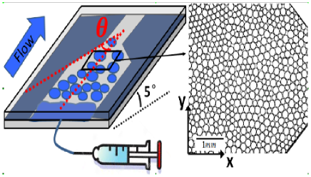
Figure 1: Schema of our sample chamber (left) and raw image of the emulsion flowing in the $+x$-direction (right). The hopper angle $\theta=54^{\circ}\pm 5^{\circ}$.

In this manuscript, we present experimental and computational studies of hopper flow of emulsion samples. Our experimental emulsions are oil droplets in water and are compressed between two parallel glass plates so that the droplets are deformed into pancake-like disks. The area fractions are all above jamming dDurian1997 . Our exit orifices are all small ($\sim 4$ droplet diameters across). We drive the flow with a pump, and given that our droplets are deformable, they cannot permanently clog at the exit. We see a range of flow behaviors. At the slowest flow rates, the flow pauses for long periods of time broken up by large avalanches of rearrangements. At higher flow rates droplets exit continuously. Intriguingly, the transition between the two flow behaviors occurs fairly smoothly as the flow rate is increased, and at moderate flow rates we see an intermediate type of flow behavior. The non-constant flow seen in the experiment is in contrast with the constant flux driving condition at the pump, indicating that the system has compliance: rather than being infinitely rigid, the system expands under pressure. Our computational studies address this using the “Durian bubble model” durian95 ; sTewari1999 , modified to mimic our experiment and with the effects of an added compliance. The simulations show the same results as the experiment: at lowest driving, the simulated compliance results in clogging and avalanches; for larger driving, we see a smooth transition to continuous flux. Our results highlight the interesting influence of compliance on the behavior of these flowing soft particles.

II Methods

II.1 Experimental samples and sample chambers

Our emulsions are mineral oil droplets in water using Fairy detergent (mass fraction 0.025) as a surfactant to prevent coalescence of the droplets kdesmond2013 ; dchen2012 . The droplets are produced using a standard co-flow micro-fluidic technique martinez2008 . The radius polydispersity of our droplets is 1% (standard deviation divided by mean). To prevent droplets from organizing into crystalline arrays, for each experiment we make a bidisperse emulsion by mixing together two separate batches of monodisperse droplets at a volume ratio of about 1:1. While each individual batch of monodisperse droplets has a low polydispersity, there is some variability between batches. The mean diameter of the large droplets is $270\pm 50~{}{\mu}$m and of the small droplets is $200\pm 40~{}{\mu}$m, and the diameter ratios of the bidisperse mixtures we form are in the range $d_{L}/d_{S}=1.5\pm 0.2$.

In our experiment, we confine droplets between two 25 mm $~{}{\times}$ 75 mm glass slides. The slides are separated by pieces of $100~{}{\mu}$m transparency film sealed with epoxy. These pieces of film act as spacers and thus create a gap between the slides. This gap ranges from 115 to 140 $~{}{\mu}$m in different experiments. This range is mainly due to the different amount of epoxy applied when making each chamber. Nonetheless, within a given sample chamber, this gap is constant with uncertainty $1.8\%$ within any given sample chamber so the slides are parallel (the corresponding maximum angle between two slides is less than $1^{\circ}$). Sample chambers for which this was not true were discarded. While the gap thickness varies from experiment to experiment, our prior work found that the thickness was unimportant as far as the contact forces droplets exert on one another when they contact kdesmond2013 . In all cases, the diameters of the oil droplets are chosen to be larger than the gap of the sample chamber. Thus, the droplets are squeezed between the two glass slides to achieve a quasi-2D system.

The left panel in Fig. 1 shows the schema of the chamber. The pieces of film are cut to form a symmetric hopper channel with angle $\theta=54\pm 5^{\circ}$ (see Fig. 1) and opening width $0.7-1$ mm. The sample chamber is tilted at an angle $5\pm 1^{\circ}$ relative to the horizontal, to use the buoyant force of the droplets to balance the viscous friction between droplets and glass slides at intermediate flow rates. The buoyant force is due to the density difference between water and mineral oil ($\rho_{\rm water}=1.00$ g/cm³, $\rho_{\rm oil}=0.83$ g/cm³). First we load the emulsion into the sample chamber, and then behind the emulsion we add pure mineral oil. A syringe pump injects additional mineral oil into the chamber at constant flux rate to push the emulsion through the chamber and thus funnel the droplets through the hopper exit. The syringe pump is connected to the chamber via Teflon tubing.

We use a microscope with a 1.6$\times$ objective lens to image the system, focusing on the chamber midplane where the 2D droplet images are clearest. A CCD camera records the images in the region close to (0.5-2 mm away from) the hopper opening. Depending on the mean speed of the flow in a given experiment, the camera frame rate is between 0.2 and 2 images/second. This is sufficient to track the trajectory of each individual droplet using standard software crocker96 , even at the maximum velocity $0.06\langle D\rangle$/s, where $\langle D\rangle$ is the mean diameter of the droplets. The right panel in Fig. 1 shows a typical raw image, in which we record hundreds of droplets within the field of view. Typically, we have 100-200 droplets in the field of view. In the 45 experiments, an average of 425 droplets are seen to exit during an experiment, although the exact amount varies from $\sim 100$ to $\sim 1000$.

II.2 Experimental control parameters

One of our main control parameters is the area fraction $\phi$ occupied by oil droplets, as measured from our image analysis. $\phi$ is somewhat controllable by what we put into the sample chamber: ahead of time, we prepare bulk emulsion samples at different 3D volume fractions. All our reported $\phi$ in this paper are the measured values from the image analysis. From the post-processed images, we observe that $\phi$ has only minimal fluctuations during an experiment, with a relative standard deviation no more than $0.5\%$. These fluctuations are primarily due to the finite field of view, with $\phi$ changing when droplets flow in and out. In flowing suspensions of solid particles there can be a self-filtration effect haw04 , but we see no evidence of this (which would be signaled by a monotonic increase of $\phi$). Additionally, we look for water flow relative to the emulsion droplets fFairbrother1935 ; fBretherton1961 by adding tracer particles to the water for a few cases. In every case, the water flows at the same rate as the oil droplets. For example, in some situations, the oil droplets cease flowing for a period of time, and during those times the water is also seen to cease flowing. There is an additional possible systematic uncertainty for $\phi$ as the apparent size of each droplet depends on the illumination settings of the microscope. We keep these settings constant between each experiment.

The other main control parameter for our experiments is the flux rate $F$. We take a total of 45 data sets with $0.83\leq\phi\leq 0.99$ and $0.0001\leq F\leq 0.02$ ml/hr. For each experiment, $F$ is set by a syringe pump and thus is constant at the pump. However, the observed flow velocity fluctuates. This is likely due to some compliance in the sample chamber, allowing sample to flow in slightly without having to flow out, and building up pressure until it is released by droplets flowing out. Therefore, rather than using $F$ to parameterize the experiments, we instead use the observed flux rate $r_{\rm expt}$, measured by the total number of droplets that exit the sample chamber divided by the total observation time.

II.3 Computational methods

As noted above, while the pump provides a constant flux rate $F$, the observed flow velocity fluctuates due to sample chamber compliance. We use a simulation to better study the importance of compliance. In particular, we use the “Durian bubble model,” introduced in durian95 . We use the version as modified in sTewari1999 to account for variable numbers of nearest neighbor particles and as further modified in hong17 to account for viscous friction between the moving droplets and the glass walls that make the experimental droplets quasi-2D. In this model, droplets are considered as disks of fixed radius $R_{i}$ (for disk $i$) with a repulsive force when they overlap, meant to approximate the influence of surface tension for real droplets. Droplet motion is assumed to be at low Reynolds number (Re $\approx 10^{-2}$ at most in our experiment), so the model sets the droplet velocity by having all repulsive droplet-droplet forces (or droplet-wall forces) balanced with the velocity-dependent viscous forces. The resulting equation is

$$\sum_{j}[\vec{F}^{\rm contact}_{ij}+\vec{F}^{\rm viscous}_{ij}]+\vec{F}^{\rm wall}_{i}+\vec{F}^{\rm driving}_{i}+\vec{F}^{\rm plates}_{i}=0.$$ (1)

The repulsive contact force between droplets $i$ and $j$ is given by

$$\vec{F}_{ij}^{\rm contact}=F_{0}\Big{[}\frac{1}{|\vec{r}_{i}-\vec{r}_{j}|}-\frac{1}{|R_{i}+R_{j}|}\Big{]}\vec{r}_{ij},$$ (2)

using the droplet radii $R_{i}$, their positions $\vec{r}_{i}$, and the vector $\vec{r}_{ij}=\vec{r}_{j}-\vec{r}_{i}$. The neighbors $j$ are defined as those droplets for which $|\vec{r}_{ij}|<R_{i}+R_{j}$, that is, overlapping circles. The repulsive wall force is similar, pointing away from the wall and using $R_{\rm wall}=0$. The viscous forces between two droplets act if they are overlapping and moving with different velocities: $\vec{F}_{ij}^{\rm viscous}=b_{\rm droplet}(\vec{v}_{j}-\vec{v}_{i})$, a force which attempts to equalize their velocities. The viscous force from the confining plates is given by $\vec{F}_{ij}^{\rm plates}=-b_{\rm plate}R^{2}_{i}\vec{v}_{i}$. As in prior work hong17 ; tao21 , we take $F_{0}=b_{\rm droplet}=b_{\rm plate}=1$, and use droplets with a Gaussian distribution of droplet sizes (mean diameter 1, standard deviation 0.1). (The desire to use a Gaussian distribution in the simulation, rather than a bidisperse distribution to better match the experiment, is that this way the simulations are consistent with our prior work hong17 ; tao21 . Also, the details of the particle size distribution should not matter that much to the overall phenomenology we’re studying; the main goal in both simulation and experiment is to avoid the particles organizing into hexagonal crystals, as they would do in a monodisperse sample.) The unit of time in the simulation is $b_{\rm droplet}\langle R\rangle/F_{0}$, the time it takes two droplets to push apart, limited by viscous drag.

The final force in the model is the driving force. To understand this force we will digress to discuss the influence of compliance on regular fluids in a microfluidic chamber, following the argument in Tabeling tabeling10 (see also martin75 ; stone04 ). Tabeling considers the case of an incompressible fluid driven by a constant flux pump at one end of a long tube with elastic wall compliance; the fluid exits the tube at the other end. Initially before the pump is started, the system has pressure $P_{0}=0$ and tube diameter $D_{0}$. When the pump drives the fluid, the pressure $P(t)$ at the pump end of the tube increases, putting stress on the tube walls. The hoop stress and axial stress are related to the pressure as

$$\sigma_{\theta\theta}=2\sigma_{zz}=\frac{D}{2T}P$$ (3)

in terms of the tube diameter $D$ and tube wall thickness $T\ll D$ timoshenko56 . (The radial stress is negligible in tubes timoshenko56 .) Positive hoop stress tries to increase the tube diameter $D$, and positive axial stress tries to increase the tube length $L$, with the amount of increase limited by the Young’s modulus $E$ for the tube material. These expansion effects are coupled via the Poisson ratio $\nu$ of the tube material, so the changes in the tube dimensions for small pressure increases are timoshenko56 :

$$\frac{\Delta L}{L}=\frac{1}{E}(\sigma_{zz}-\nu\sigma_{\theta\theta})=\frac{D}{4TE}(1-2\nu)P$$ (4)

and

$$\frac{\Delta D}{D}=\frac{1}{E}(\sigma_{\theta\theta}-\nu\sigma_{zz})=\frac{D}{4TE}(2-\nu)P.$$ (5)

The fractional change in volume is given by

$$\frac{\Delta V}{V}\approx\frac{\Delta L}{L}+2\frac{\Delta D}{D}=\frac{D}{4TE}(5-4\nu)P\equiv P/S$$ (6)

where $S\sim E$ relates to the stiffness, that is, the resistance of the tube material to stress. We can integrate both sides to relate the pressure $P(t)$ to the volume $V(t)$ as

$$P(t)=S\ln\left(\frac{V(t)}{V_{0}}\right)$$ (7)

and we see that a change in $P$ has a larger influence on $V$ when $S$ is small. This would be the case if the tube is made of a more flexible material. Note that while we have derived this for a cylindrical tube, the relation Eqn. 7 is quite general and applies for different geometries with $S\sim E$ in all cases. The exact relation between $S$ and $E$ depends on the specific geometry.

We now consider how this relation between pressure, volume, and elasticity applies to our simulation. In two dimensions, the instantaneous area of the sample chamber is $A(t)$, with $A(t)=A_{0}$ at $t=0$. The pump moves to try to create a constant flux $ra_{0}$, but initially $P\approx P_{0}=0$ so the tube expands without any fluid flowing out of the end of the tube. Here $a_{0}=\pi\langle R^{2}\rangle$ is the mean area of one droplet, so that $r$ is the number of droplets that should exit the hopper per unit time. The increasing $A(t)$ ties to an increasing pressure $P(t)$ (at the pump) and this pressure gradient then can push fluid out of the far end of the tube. There are steady-state values of $A$ and $P$ such that the flux out of the far end of the tube is $r$.

However, the simulation considers not a regular fluid but rather a collection of soft particles which are capable of clogging hong17 ; tao21 . In other words, even with $P>0$ the system may clog, causing $A$ to increase (as the pump continues moving) and increasing $P$ via Eqn. 7 such that the system eventually unclogs. To quantify this, define $A_{\rm out}(t)$ as the amount of material that has exited the system. Define

$$A_{\rm excess}(t)=ra_{0}t-A_{\rm out}(t),$$ (8)

the difference between the amount of fluid the pump has moved into the tube (area $ra_{0}t$) and the amount of fluid that has actually left the tube. Thus, the area of fluid contained in the tube is given at time $t$ by by

$$A(t)=A_{0}+A_{\rm excess}(t)$$ (9)

so that

$$A(t)/A_{0}=1+A_{\rm excess}(t)/A_{0}.$$ (10)

This expression can be put into Eqn. 7 to relate $A_{\rm out}(t)$ to the pressure $P(t)$ at the pump, causing a pressure gradient acting on each particle.

In the simulation, we treat the pressure gradient as if it is a gravitational force with strength $g(t)$, so that

$$\vec{F}^{\rm driving}_{i}(t)=g(t)R_{i}^{2}\hat{x}$$ (11)

pushes the particles toward the hopper exit. The choice of this force being proportional to $R_{i}^{2}$ is for two reasons. First, this dependence matches that of $F^{\rm plates}$ such that an isolated droplet moves with constant terminal velocity, as expected. Second, this lets us compare with our prior work which explicitly considered gravitational forces hong17 ; tao21 ; as will be demonstrated, this is a fruitful comparison that will illustrate the interplay between compliance, clogging, and avalanches.

To put this all together, Eqn. 7 is rewritten

$$g(t) = S\ln\left(1+A_{\rm excess}(t)/A_{0}\right)$$ (12)

$$\approx \ln\left(1+A_{\rm excess}(t)[S/A_{0}]\right),$$ (13)

where the approximation is valid for $A_{\rm excess}\ll A_{0}$. Given that $S$ and $A_{0}$ now appear in a ratio, we define this ratio to be the effective stiffness $s$, and rewrite Eqn. 12 as

$$g(t)=\ln\left(1+sA_{\rm excess}(t)\right).$$ (14)

In the simulation we will vary $s$ from $10^{-5}$ to $2\cdot 10^{-3}$, and in practice this equation will lead to values of $g$ in the range $g\sim 10^{-4}-10^{-1}$, consistent with our prior work which found that clogging occurs in this range hong17 . $A_{\rm out}$ increases by $\pi R_{i}^{2}$ when droplet $i$ exits; a droplet that is partially out of the hopper contributes its fractional area to $A_{\rm out}$.

To run the simulation we put 500 particles into the hopper near the exit and start with $A_{\rm excess}(t=0)=0$, $g(t=0)=0$. The hopper is set with a fixed opening width $w/d$ and stiffness $s$. $g$ then increases according to Eqns. 8, 14 using the desired flux rate $r$. Droplets that exit the hopper add their area to $A_{\rm out}(t)$; the droplets are then replaced into the hopper touching the droplets farthest away from the hopper exit, so that the number of particles remains constant. Indeed, at steady state, fluid exiting the compliant tubing would be replaced by new fluid injected by the syringe pump, keeping the total amount in the tubing constant. This choice of a constant number of droplets is equivalent to saying that $A_{\rm excess}(t)$ is always small compared to $A_{0}$.

We run the simulation using fourth-order Runge-Kutta to solve the differential equations for the droplet velocities, typically using a time step of 0.1 hong17 . We would expect there is some value of $g$ such that the time-averaged flux matches $ra_{0}$, but we would also expect that $g$ will fluctuate and that $dA_{\rm out}/dt$ will fluctuate around the value $ra_{0}$. The data are examined and the initial transient is discarded, such that for the remaining data $dA_{\rm out}/dt$ indeed fluctuates around $ra_{0}$. The simulation is then run until 1000 droplets exit the hopper.

III Experimental Results

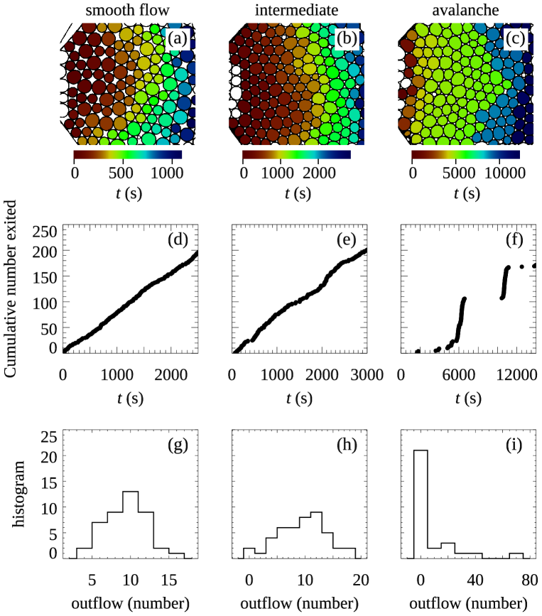
Figure 2: Description of the three flow behaviors. (a-c) Images of the samples at a particular time, with the color indicating the time when the droplet exits (see color bars). The red droplets exit earlier and blue droplets exit later. (d-f) The cumulative number of droplets that have exited the hopper as a function of time. (g-i) Histograms of the number of droplets exiting the hopper within a short time window $\Delta t$, chosen such that the mean of the histogram is 10 droplets. The flow conditions are: (a,d,g) smooth flow, $\phi=0.87$, $r_{\rm expt}=0.17$ s^-1. (b,e,h) Intermediate, $\phi=0.96$, $r_{\rm expt}=0.085$ s^-1. (c,f,i) Avalanche, $\phi=0.96$, $r_{\rm expt}=0.020$ s^-1.

We observe a wide range of flow behaviors as we vary $F$ and $\phi$ for different experiments. For large $F$, droplets flow continuously and smoothly (referred as smooth flow cases). For small $F$, we see avalanche-like flow (referred as avalanche cases). For intermediate flux rates $F$, we observe intermediate cases between these two flow patterns. As will be discussed below, we do not see any clear dependence of these flow patterns on the area fraction $\phi$.

We summarize these three flow behaviors in Fig. 2. The three pictures in Fig. 2(a)-(c) use color to show the time each droplet exits the hopper opening to the right. Red droplets exit the earliest, and blue the latest. The left picture is a smooth flow case, which shows a smooth gradient in color. The right one shows an avalanche case, where droplets have distinct groups of colors indicating that droplets exit the hopper in bursts. Note that the color scale of each plot corresponds to a different amount of time, as specified by the color bar.

Figs. 2(d)-(f) quantify these pictures by showing the cumulative number of droplets that have exited the hopper as a function of time for our three flow cases. In the smooth flow case (d), the data form a smooth curve with a well-defined slope, showing that droplets exit the hopper continuously at a fairly constant rate. The intermediate case (e) shows fluctuations in the rate, although it is still fairly continuous. In avalanche case (f), there are stretches of time where no droplets exit, followed by discrete sudden flow events where many droplets exit within a short period of time, indicated by the vertical portions of the data in (f). Specifically, the first vertical line at $t\approx 6000$ s relates to all of the light green droplets in (c) that exit at nearly the same time. Again, the existence of avalanches despite the constant flux set by the syringe pump shows that there is some compliance in the chamber, such that the pressure builds up before an avalanche.

Fig. 2(g)-(i) show the histograms of numbers of droplets that outflow within a short time window $\Delta t$. $\Delta t$ is chosen to make the mean outflow size to be 10. The smooth flow case (g) has a Gaussian shape while the avalanche case (i) has a few rare but large events. To quantify this, the skewness values for these distributions are (g) 0.15, (h) -0.03, and (i) 2.2 for smooth flow, intermediate, and avalanche cases respectively. Not surprisingly, the avalanche case has a large positive skewness, and this is generally true that all avalanche flow cases have positively skewed distributions. Given that the avalanche cases have few events overall ($\sim 100$ in some cases), our skewness data are noisy and we cannot resolve any clear trend in the skewness as a function of our control parameters. The general picture shown in Fig. 2(g)-(i) is clear, though, that avalanche cases have distributions with positive skewness and there is a trend toward more symmetric distributions with skewness $\approx 0$ as the mean flux rate $r_{\rm expt}$ increases.

To better quantify the difference of these flow behaviors, we focus on the temporal behavior of the flow. In avalanche cases, discrete sudden flow events are separated by time intervals where droplets barely move and no droplets exit the hopper. Accordingly, we define the time between two successive droplets exiting the hopper as the interval ${\Delta}t$. As shown in Fig. 3, we set $t_{1}$ as the time when the black droplet exits the hopper, $t_{2}$ as the time when the next droplet (in red) exits, and then ${\Delta}t=t_{2}-t_{1}$. In most experiments, we observe at least 100 droplets exit and thus have that many intervals. For the fastest flow rates, we have over 1000 intervals measured.

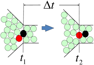
Figure 3: Schema of the definition of interval ${\Delta}t$. The left figure is at time $t_{1}$ when the black droplet exits the hopper. The right figure is at time $t_{2}$ when the red droplet exits the hopper.

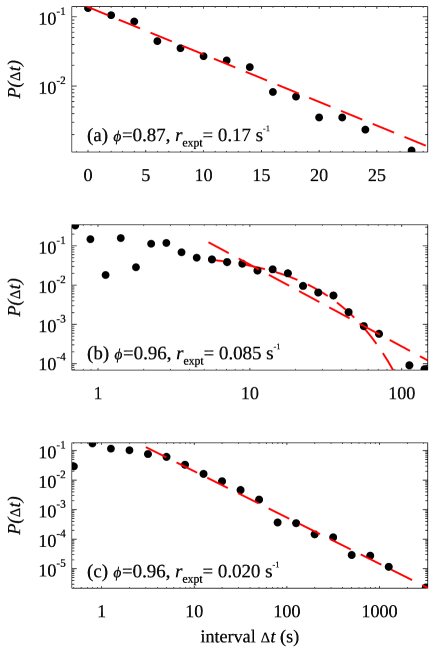
Figure 4: Typical examples of three types of probability distribution functions of ${\Delta}t$: (a) exponential distribution, (b) intermediate case, (c) power law distribution. The area fraction $\phi$ and mean flux rate $r_{\rm expt}$ are as indicated in each panel. In (a) the line shows an exponential fit $P({\Delta}t){\sim}e^{-{\Delta}t/\tau}$ with $\tau=6.3$ s. In (b) the straight line is a power-law fit $P({\Delta}t){\sim}{\Delta}t^{-\alpha}$ with $\alpha=2.1$ and the curved line is an exponential fit with $\tau=12.7$ s. In (c) the line is a power-law fit with $\alpha=1.6$.

It is apparent in the plots in Fig. 2(d-f) that the distributions of ${\Delta}t$ are different for the smooth flow and avalanche cases. In smooth flow, the values of ${\Delta}t$ are small and do not fluctuate much. In the avalanche case, ${\Delta}t$ is sometimes small (vertical portions, where many droplets exit over a short time interval) and sometimes large (horizontal stretches, where a long time passes between one droplet exiting and the next). Figure 4 shows the probability distribution functions for ${\Delta}t$ for the same three data sets shown in Fig. 2. The smooth flow case shown in Fig. 4(a) is well fit to an exponential, as shown by the dashed red line; note this is a semilog plot. The exponential fit suggests that the time between events follows a Poisson process, where events occur continuously and independently with a constant mean rate. The avalanche case shown in panel (c) is well fit to a power law, as shown by the dashed red line; note this is a log-log plot. The fit in this case is given by $P({\Delta}t){\sim}{\Delta}t^{-\alpha}$ with $\alpha=1.6$, and the power law regime covers more than 2 decades in ${\Delta}t$ and more than 4 decades in probability. The tails correspond to the long periods of time where droplets barely move. The intermediate case in panel (b) is plotted on log-log axes, and can be fit with either a power law (straight line) or an exponential (curved line); neither fit is perfect. The exponential fit fails for the largest ${\Delta}t$ while the power law is not adequate to describe the small ${\Delta}t$ region.

In our experiments we vary both $\phi$ and flux rate. For each experiment, we use the shape of $P(\Delta t)$ to describe its flow behavior. Figure 5 shows the phase diagram of fitting patterns. There is no obvious trend with $\phi$, but more clearly a transition from avalanche flow (red circles) to avalanche flow (black cross) with increasing $r_{\rm expt}$. Note that the judgment about the best fitting function is done by eye. The quality of each fit depends on which range of data is used for the fit, and while we have tried several ways to approach the fitting procedure more systematically, none seem satisfactory for the intermediate cases, and none affect the appearance of Fig. 5 in any substantial way.

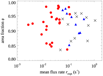
Figure 5: Phase diagram of fitting patterns of $P(\Delta t)$ in terms of area fraction $\phi$ and flux rate $r_{\rm expt}$ for our 45 experiments. Red circle: power law; blue triangle: intermediate; black cross: exponential.

The phase diagram of Fig. 5 is perhaps unsatisfying as the intermediate cases (blue triangles) are mixed in with the other two cases. However, by ignoring $\phi$ and focusing only on the flow rate dependence, the data become more unified. In particular, Fig. 6 shows the relation between the power law exponent of $P({\Delta}t)$ and $r_{\rm expt}$. The power exponent $\alpha$ increases as the flux rate increases. Even when the power law fit is not perfect (triangles), the data still follow the general trend started by the well-fit power law cases (circles). Smaller values of $\alpha$ indicate a broader distribution, where the large $\Delta t$ events are more significant: these are the avalanche cases with long pauses between short bursts when many droplets exit. This is similar to previous experimental studies of sheared granular materials, which have power law distributions of various stick-slip event properties including forces, energy, and avalanche sizes kdahmen2011 ; rCandelier2009 ; zhang2010 ; nhayman2011 ; tMajmudar2005 ; aBaldassarri2006 . Likewise, studies of clogging with sources of vibration or agitation find power law distributions of exit times janda09 ; iZuriguel2014 . To comment briefly on the exponential cases, note that the exponential fitting parameter $\tau$ corresponds to the mean interval between droplets exiting, and thus is connected to the flux rate by $\tau=1/r_{\rm expt}$.

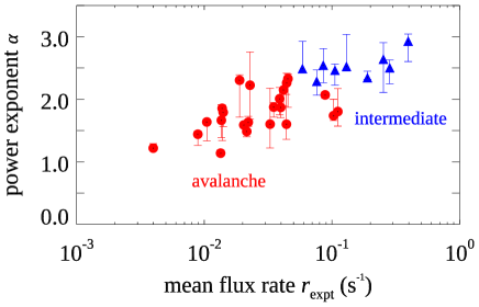
Figure 6: (a) The power law exponent $\alpha$ as a function of the experimental flux rate $r_{\rm expt}$. For the power law fits, only data in the tail are used for the fit. Different choices of the minimum $\Delta t$ used for the fit give rise to different values of $\alpha$, reflected in the error bars shown.

IV Simulation results

As described in Sec. II.3, the aim of the simulation is to describe the flow of soft 2D particles with viscous interactions and in a system with controllable compliance. From our prior work with fixed (gravitational) driving, we know that such systems can clog hong17 ; tao21 where particles stop exiting the hopper permanently. This clogging occurs more easily for narrow opening exit widths $w/d$ (in terms of the mean droplet diameter $d$). In the simulations we report here, the driving can increase indefinitely (Eqns. 8, 14) so that no clog is permanent.

Figure 7 confirms that this simulation leads to clogging and avalanche behavior. In this figure the conditions have been optimized for clogging: a small opening width $w/d$, small flux rate $r$, and small stiffness $s$ (see caption for details). The behavior of $g$ is shown in Fig. 8 ($r=0.001$ data, bottom curve). The small flux rate and small stiffness results in a repeated cycle where $g$ is small enough to cause clogging, then gradually $A_{\rm excess}$ and thus $g$ build up until the clog is disrupted and an avalanche occurs, at which point $A_{\rm excess}$ quickly decreases, decreasing $g$ so that another clog can occur. In Fig. 7 there’s an obvious division between the red and yellow droplets. The red droplets all exit the hopper before $rt\approx 100$. At $rt\approx 100$, Fig. 8 shows the start of a long nearly monotonic increase in $g$, which ends at $rt\approx 220$. This is when the yellow droplets of Fig. 7 begin to exit the hopper.

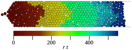
Figure 7: Image of the simulation data, colored similarly to Fig. 2 with color indicating the time when the droplet exits. For this simulation, the exit width is $w/d=1.4$ (width divided by mean droplet diameter), the flux rate is $r=10^{-3}$, and the stiffness is $s=3\cdot 10^{-5}$. The exit time distribution appears power law with exponent $\alpha=1.7$. The total time shown is $5.53\times 10^{5}$, during which given $r=10^{-3}$ we’d expect 553 droplets to flow out; only 500 droplets flow out for this particular time interval.

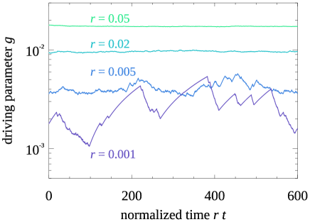
Figure 8: The value of the simulation driving parameter $g$ as a function of time. Time is normalized by the rate $r$ such that on average one droplet should exit per unit normalized time. Stretches of data where $g$ increases are due to periods where the system is clogged. The values of the rate $r$ are as indicated.

As with the experiment, the time $\Delta t$ between subsequent droplets exiting the hopper varies. Representative probability distributions for the simulation are shown in Fig. 9, where the only parameter varied is the imposed flow rate $r$ as indicated in each panel. The largest flow rate corresponds to an exponential distribution [Fig. 9(a)], the slowest flow rate corresponds to a power law distribution [Fig. 9(c)], and the intermediate flow rate is a bit hard to characterize [Fig. 9(b)].

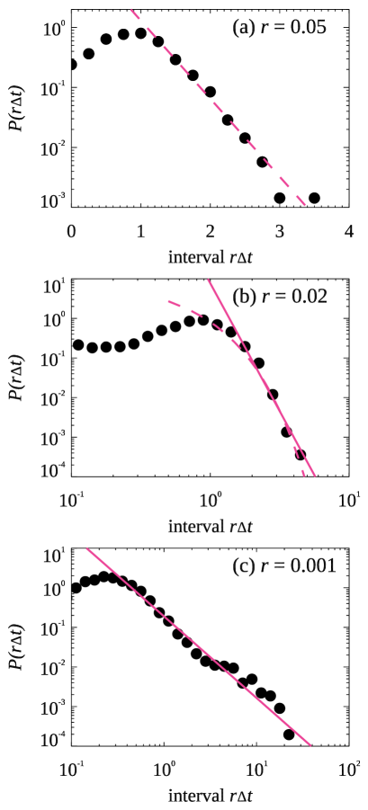
Figure 9: Typical examples of three types of probability distribution functions of $\Delta t$ from simulation data: (a) exponential distribution, (b) intermediate case, (c) power law distribution. The flux rate $r$ is as indicated, and for these data the stiffness is $s=10^{-4}$. The time is normalized by $r$, so that the mean time between droplets exiting is 1. In (b) the straight line is a power-law fit $P(\Delta t)\sim\Delta t^{-\alpha}$ with $\alpha=6.5$. In (c) the straight line is a power-law fit with $\alpha=2.1$. The dashed lines in (a) and (b) are exponential fits.

The simulation allows us to better understand how the avalanches are related to clogging. To do this we conduct a complementary set of simulations where $g$ is fixed (in other words, an infinitely stiff system [$s\rightarrow\infty$], and not using Eqn. 14) and the simulation is run until clogging is observed. As with the main simulations described in Sec. II.3, we use 500 droplets and when a droplet exits the hopper it is replaced. When a clog occurs, the clogging event is recorded, and the system is reset by removing the droplets forming the clogging arch and replacing them at the back of the hopper. A clog is defined as when no droplets exit the hopper for a long time, and the maximum velocity of any droplet falls below $10^{-5}$ hong17 . During times when clogging has not occurred, we measure the mean flux rate $\langle r\rangle$. These no-compliance results are shown in Fig. 10(a) as the solid lines – that is, these lines are the time averaged flux $\langle r\rangle$ emergent from the simulation at fixed $g$. These results are comparable to the results from the first set of simulations, plotted as symbols, where the flux rate $r$ is fixed and we measure the time averaged $\langle g\rangle$. For $r>10^{-2}$ at the right side of the graph, we get the same results whether we fix $g$ or fix $r$.

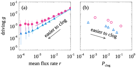
Figure 10: (a) Symbols: the mean value of the gravitational driving parameter $g$ as a function of the desired mean flux rate $r$, for $w/d=1.4$ (circles) and $w/d=2.0$ (triangles). The thin vertical lines indicate the spread from the 10%ile to 90%ile of $g$. Thick lines: the mean value of the measured flux rate $r$ from simulations with constant $g$, omitting moments when the simulation permanently clogged. (b) The horizontal axis shows the probability per droplet of a clogging event from simulations with constant gravity $g$ (vertical axis).

On the left side of the graph in Fig. 10(a), for the simulations with compliance, the mean value of $g$ is higher than we would expect for a given desired flux rate $r$ based on the no-compliance simulations. To understand this, we consider the clogging probability measured in the no-compliance simulations. We determine the mean number of droplets that flow out between clogs $\langle N\rangle$, and define $P_{\rm clog}=1/\langle N\rangle$, the mean probability of any individual droplet clogging. This probability is plotted in Fig. 10(b): to be clear, the no-compliance simulations are done with fixed $g$ (vertical axis) and we measure $P_{\rm clog}$ (horizontal axis), plotted this way to facilitate comparison with panel (a). For smaller values of $g$, clogging is easier. Additionally, for smaller opening size $w/d$, clogging is easier [red circles in Fig. 10(b)]. This then explains the flux results for small gravity (small flux) in Fig. 10(a): The “expected” value of $g$ for achieving a desired flux rate $r$ is so small that clogging easily occurs for the given opening width $w/d$. Thus $g$ rises until the clog breaks, although at that point $g$ is larger than needed for the desired flux rate $r$ and $g$ thus decreases. It is these fluctuations in $g$ that result in long-lived clogs and large avalanches. Due to the logarithm in Eqn. 14, the mean value of $g$ is higher than “expected” from simple extrapolation of the no-compliance simulation data [the solid lines in Fig. 10(a)]. The thin vertical lines in Fig. 10(a) show the variability of $g$, highlighting that the fluctuations are more significant when the desired flux rate $r$ is small. The long tails of the $P(\Delta t)$ distributions are due to unusually strong clogging arches. This suggests that the strength of an arch – how much weight it can support – may have a power law distribution as well.

Figure 10(a) also suggests that there is some threshold arch strength that must be exceeded to break the strongest arches. That is, the height of the thin vertical lines is nearly constant for low values of $r$, showing that the fluctuations in $g$ always rise above a threshold to unclog the system. This is also suggested in Fig. 8, where the two lowest rates $r$ have similar maximal values of $g$. In a sense, our clogging system is acting like a yield stress fluid coussot02 . For a yield stress fluid, if the applied stress is below the yield stress, it does not flow. The difference between a yield stress fluid and our system is that for the former the non-flowing behavior is a homogeneous bulk response from the entire material, whereas in our system the clogging is due to the few specific particles forming the arch at the exit hong17 . For this reason, in our simulation the particular yielding point (value of $g$ for which the system unclogs) varies from clog to clog, given that the arch structure is variable.

These results (clogging and time-varying forcing $g$) conceptually explain the probability distribution functions for the time intervals shown in Fig. 9. To complete the story, Fig. 11 uses the compliance simulation data to show how the measured power law exponent $\alpha$ varies with the flux rate $r$ at fixed stiffness $s$ in panel (a), and how $\alpha$ varies with $s$ at fixed $r$ in panel (b). The larger uncertainties at $r\sim 10^{-2}$ and $s\geq 10^{-3}$ indicate that the power law fits become dubious, signalling the crossover to exponential distributions. Power law exponents $\alpha>3$ are also reasonable indications of a transition to exponential distributions. The results of Fig. 11 strongly suggest that indeed it is the experimental compliance that allows for us to observe the flow rate dependent crossover from avalanche behavior to continuous flow. The values of $\alpha$ we see in the simulation are comparable with the experimental values (compare Fig. 6) at the low end; at the high end, the simulation can generate more data and thus measure power law exponents even for steeply decaying functions with $3<\alpha<6$.

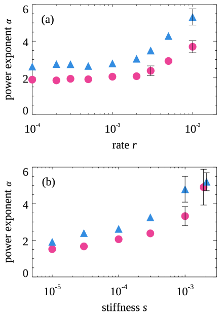
Figure 11: (a) Power-law exponent $\alpha$ as a function of flux rate $r$ from simulation data, for $w/d=1.4$ (circles) and $w/d=2.0$ (triangles). The stiffness is $s=10^{-4}$. (b) $\alpha$ as a function of stiffness $s$ for fixed flux rate $r=10^{-3}$ and the symbols indicating $w/d$ as in panel (a). For both panels, the error bars indicate the uncertainty of $\alpha$. Where not shown, the uncertainty is smaller than the symbol size.

V Conclusions

We have demonstrated that in a simple hopper geometry we see behaviors changing from clear avalanches to smooth continuous flows as we increase the mean flow rate by a factor of 100. We quantify these behaviors by examining the distributions of times $\Delta t$ between subsequent droplets exiting the hopper. Intriguingly, the transition in the flow behaviors is smooth as we increase the flow rate: the power law exponent characterizing the tails of $P(\Delta t)$ smoothly varies as the flow rate increases past the point where a power law no longer adequately describes the data [Figs. 6, 11(a)]. One possibility is that at any flow rate, the distribution $P(\Delta t)$ may be describable by a power law with an exponential cutoff, and this cutoff may smoothly move to smaller $\Delta t$ as the flow rate increases. However, the data we have for the intermediate cases [such as shown in Fig. 4(b) and Fig. 9(b)] are hard to interpret in the tails, and so it is difficult to resolve this question. The rate dependence of our observations is consistent with prior studies of athermally sheared 2D amorphous solids which demonstrated rate dependence lemaitre09 ; rWhite2003 ; gKatgert2008 ; kKrishan2008 ; rHartley2003 ; dHowell1999 ; cVeje1999 . A simulation eWoldhuis2015 based on Durian’s 2D bubble model dDurian1997 predicted a similar trend for the flow behavior as strain rate increases. However, this study also found a dependence of the transition on area fraction, which we do not see. It is likely this is due to different flow geometries (a simple shear flow in the simulation, as compared to our hopper flow which allows for clogging). The dependence on velocity is also displayed in experimental studies of sheared granular materials, where friction plays a key role jGollub1997 ; nasuno98 ; jKrim2011 . One of these studies in particular also noted that more compliant driving resulted in larger fluctuations in the sample motion nasuno98 , in agreement with our observations. For hopper flow in granular experiments, the presence of static friction can make jamming and clogging obvious, where stress-supporting solid arches form across the exit to01 ; hong17 . In addition to static friction, such experiments are also driven by a constant force (gravity), whereas in our experiments the syringe pump increases the pressure until flow occurs, and so no arches can persist indefinitely.

It is also clear from the simulations that the compliance plays an important role. By increasing the stiffness of the system [Fig. 11(b)] we can drive the system from power-law behavior to exponential behavior. While our results suggest that even for a quite stiff system there is still some hypothetical quite slow flux rate that would lead to avalanches, it is likely that such a low flux rate would be experimentally challenging to control. While our simulation method uses some approximations, the conceptual picture is simple. At slow flow rates, when the sample clogs, the pressure rises until it unclogs, and then the pressure drops to keep the mean flow rate slow. For fast flow rates, the driving pressure is such that the sample never clogs, so the flow rate is steadier.

In summary, we see that the flow of an emulsion through a hopper can vary from avalanche-like to continuous. The transition between these behaviors is not abrupt, but rather a continuous function of the flow rate. At the lowest flow rates, the power law exponent we observe approaches $\alpha=1$, showing that the flow has extremely long quiescent intervals in between the avalanches. The decrease of the power law exponent with decreasing flow rate [Figs. 6, 11(a)] suggests that even with these slow flows, we are not in a quasi-static limit, in agreement with a prior study of slowly sheared bubble rafts Twardos05 . In this simple limit where the strain rate approaches zero, the flow is not simple, but rather dominated by the rare intermittent avalanches.

References

- (1) R. Benzi, M. Sbragaglia, P. Perlekar, M. Bernaschi, S. Succi, and F. Toschi, Direct evidence of plastic events and dynamic heterogeneities in soft-glasses, Soft Matter, 10, 4615–4624 (2014).
- (2) A. D. Gopal and D. J. Durian, Nonlinear bubble dynamics in a slowly driven foam, Phys. Rev. Lett., 75, 2610–2613 (1995).
- (3) M. Dennin and C. M. Knobler, Experimental studies of bubble dynamics in a slowly driven monolayer foam, Phys. Rev. Lett., 78, 2485–2488 (1997).
- (4) S. Tewari, D. Schiemann, D. J. Durian, C. M. Knobler, S. A. Langer, and A. J. Liu, Statistics of shear-induced rearrangements in a two-dimensional model foam, Phys. Rev. E, 60, 4385–4396 (1999).
- (5) J. P. Sethna, K. A. Dahmen, and C. R. Myers, Crackling noise, Nature, 410, 242–250 (2001).
- (6) D. Fisher, K. Dahmen, S. Ramanathan, and Y. Ben-Zion, Statistics of earthquakes in simple models of heterogeneous faults, Phys. Rev. Lett., 78, 4885–4888 (1997).
- (7) K. Dahmen, D. Ertaş, and Y. Ben-Zion, Gutenberg-Richter and characteristic earthquake behavior in simple mean-field models of heterogeneous faults, Phys. Rev. E, 58, 1494–1501 (1998).
- (8) K. A. Dahmen, Y. B. Zion, and J. T. Uhl, Micromechanical model for deformation in solids with universal predictions for Stress-Strain curves and slip avalanches, Phys. Rev. Lett., 102, 175501 (2009).
- (9) S. Nasuno, A. Kudrolli, and J. Gollub, Friction in granular layers: Hysteresis and precursors, Phys. Rev. Lett., 79, 949–952 (1997).
- (10) S. Nasuno, A. Kudrolli, A. Bak, and J. P. Gollub, Time-resolved studies of stick-slip friction in sheared granula r layers, Phys. Rev. E, 58, 2161–2171 (1998).
- (11) J. Krim, P. Yu, and R. P. Behringer, Stick–Slip and the transition to steady sliding in a 2D granular medium and a fixed particle lattice, Pure and Applied Geophysics, 168, 2259–2275 (2011).
- (12) J. Urbach, R. Madison, and J. Markert, Interface depinning, self-organized criticality, and the Barkhausen effect, Phys. Rev. Lett., 75, 276–279 (1995).
- (13) I. Zuriguel, D. R. Parisi, R. C. Hidalgo, C. Lozano, A. Janda, P. A. Gago, J. P. Peralta, L. M. Ferrer, L. A. Pugnaloni, E. Clément, D. Maza, I. Pagonabarraga, and A. Garcimartín, Clogging transition of many-particle systems flowing through bottlenecks, Scientific Reports, 4, 7324 (2014).
- (14) M. Dennin, Statistics of bubble rearrangements in a slowly sheared two-dimensional foam, Phys. Rev. E, 70, 041406 (2004).
- (15) D. J. Durian, Bubble-scale model of foam mechanics:mMelting, nonlinear behavior, and avalanches, Phys. Rev. E, 55, 1739–1751 (1997).
- (16) E. Pratt and M. Dennin, Nonlinear stress and fluctuation dynamics of sheared disordered wet foam, Phys. Rev. E, 67, 051402 (2003).
- (17) Y. Bertho, C. Becco, and N. Vandewalle, Dense bubble flow in a silo: An unusual flow of a dispersed medium, Phys. Rev. E, 73, 056309 (2006).
- (18) M. Lundberg, K. Krishan, N. Xu, C. S. O’Hern, and M. Dennin, Reversible plastic events in amorphous materials., Phys. Rev. E, 77, 041505 (2008).
- (19) R. R. Hartley and R. P. Behringer, Logarithmic rate dependence of force networks in sheared granular materials, Nature, 421, 928–931 (2003).
- (20) A. Janda, I. Zuriguel, A. Garcimartín, L. A. Pugnaloni, and D. Maza, Jamming and critical outlet size in the discharge of a two-dimensional silo, Europhys. Lett., 84, 44002 (2008).
- (21) A. Janda, D. Maza, A. Garcimartín, E. Kolb, J. Lanuza, and E. Clément, Unjamming a granular hopper by vibration, Europhys. Lett., 87, 24002 (2009).
- (22) M. A. Aguirre, J. G. Grande, A. Calvo, L. A. Pugnaloni, and J. C. Géminard, Pressure independence of granular flow through an aperture, Phys. Rev. Lett., 104, 238002 (2010).
- (23) N. Hayman, L. Ducloué, K. Foco, and K. Daniels, Granular controls on periodicity of stick-slip events: Kinematics and force-chains in an experimental fault, Pure and Applied Geophysics, 168, 2239–2257 (2011).
- (24) P. Lafond, M. Gilmer, C. Koh, E. Sloan, D. Wu, and A. Sum, Orifice jamming of fluid-driven granular flow, Phys. Rev. E, 87, 042204 (2013).
- (25) T. J. Wilson, C. R. Pfeifer, N. Mesyngier, and D. J. Durian, Granular discharge rate for submerged hoppers, Papers in Physics, 6, 060009 (2014).
- (26) J. Rajchenbach, Flow in powders: From discrete avalanches to continuous regime, Phys. Rev. Lett., 65, 2221–2224 (1990).
- (27) A. W. Jenike, Quantitative design of mass-flow bins, Powder Technology, 1, 237–244 (1967).
- (28) R. M. Nedderman, U. Tuzun, S. B. Savage, and G. T. Houlsby, The flow of granular materials–I : Discharge rates from hoppers, Chem. Eng. Sci., 37, 1597–1609 (1982).
- (29) W. E. Deming and A. L. Mehring, The gravitational flow of fertilizers and other comminuted solids, Ind. Eng. Chem., 21, 661–665 (1929).
- (30) W. A. Beverloo, H. A. Leniger, and J. van de Velde, The flow of granular solids through orifices, Chem. Eng. Sci., 15, 260–269 (1961).
- (31) R. L. Brown and J. C. Richards, Two- and Three-Dimensional flow of grains through apertures, Nature, 182, 600–601 (1958).
- (32) K. To, P. Y. Lai, and H. K. Pak, Jamming of granular flow in a two-dimensional hopper, Phys. Rev. Lett., 86, 71–74 (2001).
- (33) J. Tang, S. Sagdiphour, and R. P. Behringer, Jamming and flow in 2D hoppers, AIP Conf. Proc., 1145, 515–518 (2009).
- (34) R. T. Fowler and J. R. Glastonbury, The flow of granular solids through orifices, Chem. Eng. Sci., 10, 150–156 (1959).
- (35) D. C. Hong and J. A. McLennan, Molecular dynamics simulations of hard sphere granular particles, Physica A, 187, 159–171 (1992).
- (36) D. J. Durian, Foam mechanics at the bubble scale, Phys. Rev. Lett., 75, 4780–4783 (1995).
- (37) K. W. Desmond, P. J. Young, D. Chen, and E. R. Weeks, Experimental study of forces between quasi-two-dimensional emulsion droplets near jamming, Soft Matter, 9, 3424–3436 (2013).
- (38) D. Chen, K. W. Desmond, and E. R. Weeks, Topological rearrangements and stress fluctuations in quasi-two-dimensional hopper flow of emulsions, Soft Matter, 8, 10486–10492 (2012).
- (39) R. Shah, H. Shum, A. Rowat, D. Lee, J. Agresti, A. Utada, L. Chu, J. Kim, A. Fernandez-Nieves, and C. Martinez, Designer emulsions using microfluidics, Materials Today, 11, 18–27 (2008).
- (40) J. C. Crocker and D. G. Grier, Methods of digital video microscopy for colloidal studies, J. Colloid Interface Sci., 179, 298–310 (1996).
- (41) M. D. Haw, Jamming, two-fluid behavior, and “self-filtration” in concentrated particulate suspensions, Phys. Rev. Lett., 92, 185506 (2004).
- (42) F. Fairbrother and A. E. Stubbs, Studies in electro-endosmosis. Part VI. The “bubble-tube” method of measurement, J. Chem. Soc., pages 527–529 (1935).
- (43) F. P. Bretherton, The motion of long bubbles in tubes, J. Fluid Mech., 10, 166–188 (1961).
- (44) X. Hong, M. Kohne, M. Morrell, H. Wang, and E. R. Weeks, Clogging of soft particles in two-dimensional hoppers, Phys. Rev. E, 96, 062605 (2017).
- (45) R. Tao, M. Wilson, and E. R. Weeks, Soft particle clogging in two-dimensional hoppers, Phys. Rev. E, 104, 044909–044909 (2021).
- (46) P. Tabeling, Introduction to Microfluidics (Oxford University Press, Oxford), reprint edition edition (2010), ISBN 978-0-19-958816-9.
- (47) M. Martin, G. Blu, C. Eon, and G. Guiochon, The use of syringe-type pumps in liquid chromatography in order to achive a constant flow-rate, J. Chrom. A, 112, 399–414 (1975).
- (48) H. A. Stone, A. D. Stroock, and A. Ajdari, Engineering flows in small devices, Ann. Rev. Fluid Mech., 36, 381–411 (2004).
- (49) S. Timoshenko, Strength of Materials Part I, 2nd ed. (D. Van Nostrand Company, Inc.) (1940).
- (50) K. A. Dahmen, Y. Ben-Zion, and J. T. Uhl, A simple analytic theory for the statistics of avalanches in sheared granular materials, Nat. Phys., 7, 554–557 (2011).
- (51) R. Candelier, O. Dauchot, and G. Biroli, The building blocks of dynamical heterogeneities in dense granular media, Phys. Rev. Lett., 102, 088001 (2009).
- (52) J. Zhang, T. S. Majmudar, A. Tordesillas, and R. P. Behringer, Statistical properties of a 2D granular material subjected to cyclic shear, Granular Matter, 12, 159–172 (2010).
- (53) T. S. Majmudar and R. P. Behringer, Contact force measurements and stress-induced anisotropy in granular materials, Nature, 435, 1079–1082 (2005).
- (54) A. Baldassarri, F. Dalton, A. Petri, S. Zapperi, G. Pontuale, and L. Pietronero, Brownian forces in sheared granular matter, Phys. Rev. Lett., 96, 118002 (2006).
- (55) P. Coussot, Q. Nguyen, H. Huynh, and D. Bonn, Avalanche behavior in yield stress fluids, Phys. Rev. Lett., 88, 175501–175501 (2002).
- (56) A. Lemaître and C. Caroli, Rate-dependent avalanche size in athermally sheared amorphous solids, Phys. Rev. Lett., 103, 065501 (2009).
- (57) R. White and K. Dahmen, Driving rate effects on crackling noise, Phys. Rev. Lett., 91, 085702 (2003).
- (58) G. Katgert, M. Möbius, and M. van Hecke, Rate dependence and role of disorder in linearly sheared two-dimensional foams, Phys. Rev. Lett., 101, 058301 (2008).
- (59) K. Krishan and M. Dennin, Viscous shear banding in foam, Phys. Rev. E, 78, 051504 (2008).
- (60) D. Howell, R. P. Behringer, and C. Veje, Stress fluctuations in a 2D granular couette experiment: A continuous transition, Phys. Rev. Lett., 82, 5241–5244 (1999).
- (61) C. Veje, D. Howell, and R. Behringer, Kinematics of a two-dimensional granular couette experiment at the transition to shearing, Phys. Rev. E, 59, 739–745 (1999).
- (62) E. Woldhuis, V. Chikkadi, M. S. van Deen, P. Schall, and M. van Hecke, Fluctuations in flows near jamming, Soft Matter (2015).
- (63) M. Twardos and M. Dennin, Comparison between step strains and slow steady shear in a bubble raft, Phys. Rev. E, 71, 061401 (2005).