Third order nonlinearity of graphene: effects of phenomenological relaxation and finite temperature

Abstract

We investigate the effect of phenomenological relaxation parameters on the third order optical nonlinearity of doped graphene by perturbatively solving the semiconductor Bloch equation around the Dirac points. An analytic expression for the nonlinear conductivity at zero temperature is obtained under the linear dispersion approximation. With this analytic formula as starting point, we construct the conductivity at finite temperature and study the optical response to a laser pulse of finite duration. We illustrate the dependence of several nonlinear optical effects, such as third harmonic generation, Kerr effects and two photon absorption, parametric frequency conversion, and two color coherent current injection, on the relaxation parameters, temperature, and pulse duration. In the special case where one of the electric fields is taken as a dc field, we investigate the dc-current and dc-field induced second order nonlinearities, including dc-current induced second harmonic generation and difference frequency generation.

I Introduction

The optical nonlinearities of monolayer graphene have recently attracted wide attention Castro Neto et al. (2009); Bonaccorso et al. (2010); Gu et al. (2012), both experimentally and theoretically. The nonlinear susceptibility of graphene Glazov and Ganichev (2014) is both strong – per atom it is orders of magnitude higher than that of common gapped semiconductors and metals – and controllable by the chemical potential Cheng et al. (2014a, b), which can be tuned by an external gate voltage Novoselov et al. (2004); Wang et al. (2008) or chemical doping Liu et al. (2011a). With the possibilities it offers for integration in silicon-based optical integrated circuits, graphene is an exciting new candidate for enhancing nonlinear optical functionalities in silicon-based on-chip optical devices, such as on-chip broadband light sources, electro-optic modulators Wülbern et al. (2010); Matheisen et al. (2014), optical switches Ironside et al. (1993); Liu et al. (2014); Gandomkar and Ahmadi (2011), and optical transistors Hagan et al. (1994); Ren et al. (2013). In realizing some of these devices Gandomkar and Ahmadi (2011), the presence of second order optical nonlinearities, especially second harmonic generation (SHG), is a key requirement.

The third order optical nonlinearity is described by the susceptibility tensor $\chi^{(3)}(\omega_{1},\omega_{2},\omega_{3})$ or equivalently the conductivity tensor $\sigma^{(3)}(\omega_{1},\omega_{2},\omega_{3})$, which has a complex frequency dependence. It describes different physical effects, such as third harmonic generation (THG), which is determined by $\chi^{(3)}(\omega,\omega,\omega)$; Kerr effects and two photon absorption, which are determined by $\chi^{(3)}(-\omega,\omega,\omega)$; two-color coherent current injection, which is determined by $\chi^{(3)}(-\omega,-\omega,2\omega)$; and parametric frequency conversion (four wave mixing), which is determined by $\chi^{(3)}(-\omega_{s},\omega_{p},\omega_{p})$. Due to the inversion symmetry of its crystal structure, pristine graphene has no second order optical nonlinearities arising from electric dipole transitions. However, in graphene-based photonic devices an effective second order susceptibility can arise from the breaking of inversion symmetry in a number of ways: (1) the presence of an asymmetric interface between graphene and the substrate Dean and van Driel (2009, 2010); Bykov et al. (2012); An et al. (2013, 2014); Sipe et al. (1987), not relevant for normally incident light; (2) the contribution of forbidden transitions involving the finite wave vector of light Mikhailov (2007); Mikhailov and Ziegler (2008); Glazov (2011); Mikhailov (2011); Glazov and Ganichev (2014); (3) the presence of natural curvature fluctuations of suspended graphene Lin et al. (2014); (4) the application of a dc electric field to generate an asymmetric steady state Wu et al. (2012); Bykov et al. (2012); Avetissian et al. (2012a); An et al. (2013, 2014); Cheng et al. (2014b). The last is associated with the third order optical nonlinearity $\chi^{(3)}(\omega_{1},\omega_{2},0)$, with one of the electric fields independent of time. It includes current induced second harmonic generation Khurgin (1995) (CSHG) or electric field induced second harmonic generation (EFISH).

Experimental studies of many of the optical nonlinear effects mentioned above have already demonstrated in graphene. Typically the experimental data are analyzed by extracting an effective optical nonlinear susceptibility, with the graphene monolayer treated as a thin film with a thickness of $3.3$ ÅHendry et al. (2010); Säynätjoki et al. (2013); Kumar et al. (2013). In this way, most of the experimental techniques used to determine the nonlinear optical response of bulk materials or thin films can be directly applied to the study of graphene. In a gapped semiconductor, third order susceptibilities do not change drastically in the nonresonant regime, where all photon energies are much lower than the energy gap Boyd (2008). Yet they show a strong and complicated photon energy dependence in pristine graphene because resonant transitions always exist for any photon energy, due to the vanishing gap and the presence of free carriers, leading to some similarities with a metal film Kumar et al. (2013). These complexities have been observed in experimental studies of parametric frequency conversion Hendry et al. (2010), THG Säynätjoki et al. (2013); Kumar et al. (2013); Hong et al. (2013), Kerr effects and two photon absorption Yang et al. (2011); Zhang et al. (2012); Gu et al. (2012); Wu et al. (2011), two color coherent control Sun et al. (2010, 2012a, 2012b), and SHG Dean and van Driel (2009, 2010); Bykov et al. (2012); An et al. (2013, 2014); Lin et al. (2014) in graphene.

Theoretically, the optical nonlinearities of graphene have been investigated by perturbative treatments based on Fermi’s Golden Rule, and by density matrix calculations, both of which are standard methods in studying the optical response of gapped semiconductors. In an earlier communication we sketched some of the relevant work done before early 2014 ; recent contributions include a calculation by Mikhailov Mikhailov (2014) of THG , and numerically solution of the equation of motion under strong laser fields by Avetissian et al. Avetissian et al. (2012b, a, 2013a, 2013b). All of these studies focused on one or a few nonlinear effects. In our earlier work Cheng et al. (2014a) we performed a perturbative calculation based on a density matrix formalism; ignoring all scattering effects, we obtained an analytic expression for the general optical sheet conductivity $\sigma^{(3)}(\omega_{1},\omega_{2},\omega_{3})$, which can be related to the effective susceptibility $\chi^{(3)}(\omega_{1},\omega_{2},\omega_{3})$, in doped graphene at zero temperature. We found that the optical conductivities depend strongly on the chemical potential and photon energies, and exhibit many divergences associated with resonant transitions, which occur when photon energies or their combinations match the chemical potential gap. Taking $\omega_{3}=0$ and including phenomenological relaxation times for the generation of both dc and optically induced current, we calculated the current induced second order nonlinearities at zero temperature and obtained an analytic expression Cheng et al. (2014b) for CSHG. The effective susceptibility shows two peaks corresponding to two resonant transitions induced by the fundamental and the second harmonic light, with the peak values strongly dependent on the relaxation time. Adopting the parameters used in calculations of bilayer graphene Wu et al. (2012), we obtained a prediction of a peak susceptibility in monolayer graphene that was similar to that predicted for the bilayer; the EFISH contribution was ignored in that calculation.

The importance of the relaxation time demonstrated in that study, and the desire for more realistic calculations to compare with experiment, motivates the present work. Here we consider the inclusion of scattering effects in the semiconductor Bloch equations (SBE) within a relaxation time approximation, allow for finite temperature to the extent that it affects the initial state, and explicitly consider the nonlinear response to pulses of light. We obtain an analytic expression for the full nonlinear optical conductivity $\sigma^{(3)}(\omega_{1},\omega_{2},\omega_{3})$ for optical transitions around the Dirac points. We discuss the predictions that follow from this expression for different optical effects, and we compare with experiment where possible.

Our focus in this work is on doped graphene, where the chemical potential $\mu\neq 0$. However, the chemical potential dependence of our general expression for $\sigma^{(3)}(\omega_{1},\omega_{2},\omega_{3})$ allows us to study the special case of $\mu\to 0$. At the very least we might expect that, for electrons close to the Dirac points, the distinction between “interband” and “intraband” motion could be lost. Although different terms that are nominally associated with interband and intraband motion arise naturally in the development of the perturbation series, the distinction between those two “kinds” of motion is at best approximate Aversa and Sipe (1995), and we indeed find that the way those different formal terms contribute to the final result for small $\mu$ is nontrivial. More importantly, we generally associate the validity of a perturbative expansion of the optical response with the assumption that the energy induced by the presence of the optical field is much less than the energy difference between the bands. In graphene this is always violated for some states around the Dirac points, regardless of the strength of the optical field. If these states are occupied by electrons, as they are in undoped graphene, the reasonableness of a perturbative expansion is in doubt. Indeed, even a semiclassical treatment of the response to an applied electric field of electrons near the Dirac points exhibits a breakdown of the perturbative analysis Mikhailov (2007) as $\mu\to 0$. We find evidence of the same kind of behavior in the quantum treatment presented here. This has consequences even for doped graphene if finite temperature is considered, for thermal fluctuations always place some electrons near the Dirac points.

We organize our paper as follows: In Section II we introduce the SBE and our approximations for including scattering effects; the details of the derivation of the nonlinear optical conductivity is given in Appendix A. The last two subsections of Section II address the extension of the calculation to finite temperature, and the treatment of the response to a pulse with finite duration. In Section III we discuss the third order nonlinear effects, including THG, Kerr effects and two photon absorption, two-color coherent current injection, and parametric frequency conversion; in Section IV we discuss the current-induced second order nonlinearities, including CSHG, EFISH, and the nonlinear optical conductivity $\sigma^{(3)}(-\omega_{s},\omega_{p},0)$ that describes current-induced difference frequency generation. Throughout the sections we compare with experimental results when appropriate. We conclude in Section V.

II Model

We take the Hamiltonian of graphene to be

$$H=H_{0}+H_{eR}+H_{ep}+H_{ei}+H_{ee}\,,$$ (1)

Here $H_{0}$ is the unperturbed electron Hamiltonian,

$$H_{0}=\sum_{s}\int d\bm{k}\varepsilon_{s\bm{k}}a_{s\bm{k}}^{{\dagger}}a_{s\bm{k}}\,,$$ (2)

where the $a_{s\bm{k}}$ are annihilation operators of Bloch states $|s\bm{k}\rangle$ for band $s$ and wave vector $\bm{k}$, with eigen energy $\varepsilon_{s\bm{k}}$. Here $H_{eR}$ describes the interaction with radiation and in the dipole limit, where the electric field $\bm{E}(t)$ is approximated as uniform, we have

$$H_{eR}=-e\bm{E}(t)\cdot\sum_{s_{1}s_{2}}\int d\bm{k}a_{s_{1}\bm{k}}^{{\dagger}}\big{(}\bm{\xi}_{s_{1}s_{2}\bm{k}}+i\delta_{s_{1}s_{2}}\bm{\nabla}_{\bm{k}}\big{)}a_{s_{1}\bm{k}}\,,$$ (3)

where $e=-|e|$ and

$$\bm{\xi}_{s_{1}s_{2}\bm{k}}=i\int_{\text{cell}}\frac{d\bm{r}}{{\cal A}_{\text{cell}}}u_{s_{1}\bm{k}}^{\ast}(\bm{r})\bm{\nabla}_{\bm{k}}u_{s_{2}\bm{k}}(\bm{r})$$ (4)

is the Berry connection between states $|s_{1}\bm{k}\rangle$ and $|s_{2}\bm{k}\rangle$, with ${\cal A}_{\text{cell}}$ the unit cell area and $u_{s\bm{k}}(\bm{r})$ the periodic part of the Bloch function, $\langle\bm{r}|s\bm{k}\rangle=(2\pi)^{-1}e^{i\bm{k}\cdot\bm{r}}u_{s\bm{k}}(\bm{r},z)$, where $\bm{k}=(k_{x},k_{y})$ and $\bm{r}=(x,y)$; the graphene is assumed to lie in the $x-y$ plane. We neglect any response of the system to electric field components in the $z$ direction. The scattering terms are given by $H_{ei}$ for the electron-impurity scattering, $H_{ep}$ for the electron-phonon interaction, and $H_{ee}$ for the carrier-carrier scattering.

The system is described by a density matrix that is initially diagonal both in band index and (continuous) wave vector, $\left\langle a_{s_{1}{\bm{k}}_{1}}^{{\dagger}}a_{s_{2}{\bm{k}}_{2}}\right\rangle_{t=-\infty}=n_{s_{1}{\bm{k}}_{1}}\delta_{s_{1}s_{2}}\delta({\bm{k}}_{1}-{\bm{k}}_{2})$, where $0\leq n_{s_{1}{\bm{k}}_{1}}\leq 1$ describes the initial occupation of the state. In the presence of an applied uniform electric field it remains diagonal in ${\bm{k}}_{1}$ and ${\bm{k}}_{2}$ but can acquire off-diagonal elements in $s_{1}$ and $s_{2}$, describing the correlation between state amplitudes for $\left|s_{1}{\bm{k}}_{1}\right\rangle$ and $\left|s_{2}{\bm{k}}_{2}\right\rangle$, $\left\langle a_{s_{1}{\bm{k}}_{1}}^{\dagger}a_{s_{2}{\bm{k}}_{2}}\right\rangle_{t}=\rho_{s_{1}s_{2}{\bm{k}}_{1}}(t)\delta({\bm{k}}_{1}-{\bm{k}}_{2})$. We can think of $\rho_{s_{1}s_{2}{\bm{k}}}(t)$ as the elements of a $2\times 2$ matrix $\rho_{{\bm{k}}}(t)$, and their dynamics are determined by the SBE

$$\hbar\frac{\partial\rho_{s_{1}s_{2}\bm{k}}}{\partial t} = -i(\varepsilon_{s_{1}\bm{k}}-\varepsilon_{s_{2}\bm{k}})\rho_{s_{1}s_{2}\bm{k}}$$ (5)

$$+ ieE^{a}(t)\sum_{s}\left(\xi_{s_{1}s\bm{k}}^{a}\rho_{ss_{2}\bm{k}}-\rho_{s_{1}s\bm{k}}\xi_{ss_{2}\bm{k}}^{a}\right)$$

$$- eE^{a}(t)\frac{\partial\rho_{s_{1}s_{2}\bm{k}}}{\partial k_{a}}+\hbar\left.\frac{\partial\rho_{s_{1}s_{2}\bm{k}}}{\partial t}\right|_{\text{scat}}\,.$$

Here $\left.\frac{\partial\rho_{s_{1}s_{2}\bm{k}}}{\partial t}\right|_{\text{scat}}$ includes the scattering terms induced by $H_{ei}+H_{ep}+H_{ee}$, which could in principle be obtained from well-established treatments of many-particle systems, such as the many-particle density-matrix framework Haug and Koch (2004); Malic et al. (2011) or the Keldysh Green function method Haug and Jauho (2007). In an ordinary semiconductor with parabolic band structure, the current relaxation is mostly caused by carrier-phonon and carrier-impurity scattering, while carrier-carrier interactions are less significant due to the approximate equivalence of momentum conservation and velocity conservation. However, the novel linear band structure of graphene breaks this equivalence, and the carrier-carrier interactions play an important role in current relaxation Malic et al. (2011); Zhang and Wu (2013); thus the full expression for the scattering terms is complicated and even hard to solve numerically Haug and Jauho (2007).

We proceed in the standard way by assuming the validity of a perturbation expansion

$$\rho_{s_{1}s_{2}\bm{k}}(t)=\sum_{n=0}^{\infty}\rho_{s_{1}s_{2}\bm{k}}^{(n)}(t)\,,$$ (6)

with $\rho_{s_{1}s_{2}\bm{k}}^{(n)}(t)\propto E^{n}$. Here $\rho_{s_{1}s_{2}\bm{k}}^{(0)}(t)=\rho_{s_{1}s_{2}\bm{k}}^{0}=\delta_{s_{1}s_{2}}n_{s_{1}\bm{k}}$ is the density operator characterizing the equilibrium occupation of single-particle states at finite temperature $T$ and chemical potential $\mu$, $n_{s\bm{k}}=[1+e^{(\varepsilon_{s\bm{k}}-\mu)/(k_{B}T)}]^{-1}$ is the Fermi-Dirac distribution with $\beta=1/(k_{B}T)$ where $k_{B}$ is Boltzmann’s constant. From Eq. (5), $\rho_{s_{1}s_{2}\bm{k}}^{(n)}(t)$ satisfies

$$\hbar\frac{\partial\rho_{s_{1}s_{2}\bm{k}}^{(n)}}{\partial t} = -i(\varepsilon_{s_{1}\bm{k}}-\varepsilon_{s_{2}\bm{k}})\rho_{s_{1}s_{2}\bm{k}}^{(n)}$$ (7)

$$+ ieE^{a}(t)\sum_{s}\left(\xi_{s_{1}s\bm{k}}^{a}\rho_{ss_{2}\bm{k}}^{(n-1)}-\rho_{s_{1}s\bm{k}}^{(n-1)}\xi_{ss_{2}\bm{k}}^{a}\right)$$

$$- eE^{a}(t)\frac{\partial\rho_{s_{1}s_{2}\bm{k}}^{(n-1)}}{\partial k_{a}}+\hbar\left.\frac{\partial\rho_{s_{1}s_{2}\bm{k}}^{(n)}}{\partial t}\right|_{\text{scat}}\,,$$

where $\rho^{(n)}_{\bm{k}}\equiv 0$ for $n<0$. As a very rough approximation, a relaxation time approximation Zhang and Wu (2013) can be adopted to give

$$\hbar\left.\frac{\partial\rho_{s_{1}s_{2}\bm{k}}^{(n)}}{\partial t}\right|_{\text{scat}}=-\Gamma_{s_{1}s_{2}\bm{k}}^{(n)}\rho_{s_{1}s_{2}\bm{k}}^{(n)}\,,\text{ for }n\geq 1.$$ (8)

Here $\Gamma_{s_{1}s_{2}\bm{k}}^{(n)}$ is a relaxation parameter introduced to describe the dynamics of $\rho_{s_{1}s_{2}\bm{k}}^{(n)}(t)$, and $\hbar/\Gamma_{s_{1}s_{2}\bm{k}}^{(n)}$ corresponds to a phenomenological relaxation time. In a real system, $\Gamma_{s_{1}s_{2}\bm{k}}^{(n)}$ can be expected to depend on the temperature, chemical potential, and external field Ando et al. (2002). Yet because the relaxation plays an important role in optical nonlinearities around resonant transitions, the extremely phenomenological treatment Mermin (1970) in Eq. (8) can still reveal part of the physics, and in a very simple way. Even with the use of the six phenomenological constants $\Gamma_{s\bar{s}\bm{k}}^{(n)}=\Gamma_{e}^{(n)}$ for interband transitions and $\Gamma_{ss\bm{k}}^{(n)}=\Gamma_{i}^{(n)}$ for intraband transitions, we are still able to obtain an analytic result for the perturbation calculation within the linear dispersion approximations around the Dirac points at zero temperature. From $\rho_{\bm{k}}^{(n)}(t)$, the (areal) current density, which in our model has only $x$ and $y$ components, is calculated as $J^{d}(t)=\sum_{n=1}^{\infty}J^{(n);d}(t)$ with

$$J^{(n);d}(t)=e\sum_{s_{1}s_{2}}\int\frac{d\bm{k}}{4\pi^{2}}v_{s_{2}s_{1}\bm{k}}^{d}\rho_{s_{1}s_{2}\bm{k}}^{(n)}(t)\,.$$ (9)

We give the derivation in Appendix A, where the spin degeneracy is included. We extract the linear optical conductivity $\sigma^{(1);da}(\omega)$ from

$$J^{(1);d}(t)=\int\frac{d\omega}{2\pi}\sigma^{(1);da}(\omega)E^{a}(\omega)e^{-i\omega t}\,,$$ (10)

where $E^{a}(\omega)=\int dtE^{a}(t)e^{i\omega t}$. In graphene, the hexagonal lattice has $D_{6h}$ (6/mmm) symmetry Sutherland (2003), and there is only one independent nonzero component $\sigma^{(1);xx}=\sigma^{(1);yy}$. We first consider the zero temperature results. In this paper, we restrict ourselves to the neighborhood of the Dirac points (see Fig. 1), assuming a linear dispersion relation with two relevant bands that we label $s=+$ (upper) and $-$ (lower). We recover the usual result Ando et al. (2002); Mikhailov and Ziegler (2007)

$$\sigma^{(1);xx}(\omega)=\frac{i\sigma_{0}}{\pi}\left[\frac{4|\mu|}{\hbar\omega+i\Gamma_{i}^{(1)}}-{\cal G}_{\mu}\left(\hbar\omega+i\Gamma_{e}^{(1)}\right)\right]\,.$$ (11)

Here $\sigma_{0}={e^{2}}/{(4\hbar)}$ is the universal conductivity, and ${\cal G}_{\mu}(\vartheta)$ with $\vartheta=\vartheta_{r}+i\vartheta_{i}$ is

$${\cal G}_{\mu}(\vartheta) = \ln\left|\frac{2|\mu|+\vartheta}{2|\mu|-\vartheta}\right|+i\left(\pi+\arctan\frac{\vartheta_{r}-2|\mu|}{\vartheta_{i}}\right.$$ (12)

$$\left.-\arctan\frac{\vartheta_{r}+2|\mu|}{\vartheta_{i}}\right)\,.$$

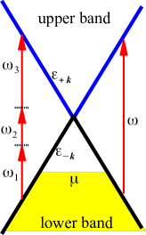
Figure 1: (color online) Illustration of the linear dispersion approximation of the graphene band structure around the Dirac point. The arrows show optical transitions induced by one photon with energy $\hbar\omega$ (right) or three photons with energy $\hbar\omega_{i}$ (left).

The third order current is given as

$$J^{(3);d}(t) = \int\frac{d\omega_{1}d\omega_{2}d\omega_{3}}{(2\pi)^{3}}\sigma^{(3);dabc}(\omega_{1},\omega_{2},\omega_{3})$$ (13)

$$\times E^{a}(\omega_{1})E^{b}(\omega_{2})E^{c}(\omega_{3})e^{-i(\omega_{1}+\omega_{2}+\omega_{3})t}\,,$$

Here the symmetrized third order optical conductivity $\sigma^{(3);dabc}$ is

$$\sigma^{(3);dabc}(\omega_{1},\omega_{2},\omega_{3})$$ (14)

$$= \frac{1}{6}\bigg{[}\widetilde{\sigma}^{(3);dabc}(\omega_{1},\omega_{2},\omega_{3})+\widetilde{\sigma}^{(3);dbca}(\omega_{2},\omega_{3},\omega_{1})$$

$$+\widetilde{\sigma}^{(3);dcab}(\omega_{3},\omega_{1},\omega_{2})+\widetilde{\sigma}^{(3);dacb}(\omega_{1},\omega_{3},\omega_{2})$$

$$+\widetilde{\sigma}^{(3);dcba}(\omega_{3},\omega_{2},\omega_{1})+\widetilde{\sigma}^{(3);dbac}(\omega_{2},\omega_{1},\omega_{3})\bigg{]}\,,$$

where the unsymmetrized third order optical conductivity is given as

$$\widetilde{\sigma}^{(3);dabc}(\omega_{1},\omega_{2},\omega_{3})$$ (15)

$$= i\sigma_{3}\Bigg{[}\frac{{\cal S}_{1}^{dabc}}{\nu\nu_{0}\nu_{3}}+\frac{{\cal S}_{2}^{dabc}(\vartheta_{3})}{\nu\nu_{0}}+\frac{{\cal S}_{3}^{dabc}(\vartheta_{0})}{\nu\nu_{3}}$$

$$\quad+\frac{{\cal S}_{4}^{dabc}(\vartheta_{0},\vartheta_{3})}{\nu}+\frac{{\cal S}_{5}^{dabc}(\vartheta)}{\nu_{0}\nu_{3}}+\frac{{\cal S}_{6}^{dabc}(\vartheta,\vartheta_{3})}{\nu_{0}}$$

$$\quad+\frac{{\cal S}_{7}^{dabc}(\vartheta,\vartheta_{0})}{\nu_{3}}+{\cal S}_{8}^{dabc}(\vartheta,\vartheta_{0},\vartheta_{3})\Bigg{]}\,,$$

with $\sigma_{3}\equiv{\sigma_{0}(\hbar v_{F}e)^{2}}/{\pi}$, $\nu_{3}\equiv\hbar\omega_{3}+i\Gamma_{i}^{(1)}$, $\vartheta_{3}\equiv\hbar\omega_{3}+i\Gamma_{e}^{(1)}$, $\nu_{0}\equiv\hbar\omega_{0}+i\Gamma_{i}^{(2)}$, $\vartheta_{0}\equiv\hbar\omega_{0}+i\Gamma_{e}^{(2)}$, $\nu\equiv\hbar\omega+i\Gamma_{i}^{(3)}$, $\vartheta\equiv\hbar\omega+i\Gamma_{e}^{(3)}$, $\omega_{0}\equiv\omega_{2}+\omega_{3}$, and $\omega\equiv\omega_{1}+\omega_{0}$. We have followed the standard convention of nonlinear optics Boyd (2008) in symmetrizing the terms $\widetilde{\sigma}^{(3);ijkl}(\omega_{j},\omega_{k},\omega_{l})$ by permuting the indices $(jkl)$ to arrive at the nonlinear conductivity $\sigma^{(3);dabc}(\omega_{1},\omega_{2},\omega_{3})$. The light-matter interaction in Eq. (3) can be formally separated into an interband contribution ($s_{1}\neq s_{2}$) and an intraband contribution ($s_{1}=s_{2}$ ), and the terms proportional to the different $\mathcal{S}_{i}$ in $\widetilde{\sigma}^{(3);dabc}$ can be classified according to how many times each contribution appears Aversa and Sipe (1995). The term proportional to ${\cal S}_{1}$ arises from only the intraband contributions, and the term proportional to ${\cal S}_{6}$ arises from only the interband contributions; all others involve mixtures of both. The quantities ${\cal S}_{i}^{dabc}$, $\widetilde{\sigma}^{(3);dabc}$, and $\sigma^{(3);dabc}$ are all fourth order tensors. Neglecting the optical response in the $z$ direction, there are in all 8 nonzero components for the $D_{6h}$ symmetry, among which three are independent; they are

$${\sigma}^{(3);xxyy} = {\sigma}^{(3);yyxx}\,,$$

$${\sigma}^{(3);xyxy} = {\sigma}^{(3);yxyx}\,,$$

$${\sigma}^{(3);xyyx} = {\sigma}^{(3);yxxy}\,,$$ (16)

and

$${\sigma}^{(3);xxxx} = {\sigma}^{(3);yyyy}$$ (17)

$$= {\sigma}^{(3);xxyy}+{\sigma}^{(3);xyxy}+{\sigma}^{(3);xyyx}\,.$$

In the following, we write the independent nonzero components of fourth rank tensors as column vectors, ordering the independent components of a fourth rank tensor $T^{dabc}$ as $T=\begin{bmatrix}T^{(3);xxyy}\\ T^{(3);xyxy}\\ T^{(3);xyyx}\end{bmatrix}$. By employing the constant vectors

$$A_{1}=\begin{bmatrix}-3\\ 1\\ 1\end{bmatrix}\,,A_{2}=\begin{bmatrix}1\\ -3\\ 1\end{bmatrix}\,,A_{3}=\begin{bmatrix}1\\ 1\\ -3\end{bmatrix}\,,A_{0}=\begin{bmatrix}1\\ 1\\ 1\end{bmatrix}\,,$$ (18)

where note $A_{0}=-(A_{1}+A_{2}+A_{3})$, we can present the analytic expression for the different components of $\widetilde{\sigma}^{(3);dabc}$ appearing in Eq. (15) at zero temperature, using the approximation of a linear dispersion relation around the Dirac points, as

$${\cal S}_{1} = \frac{1}{|\mu|}A_{0}\,,$$ (19)

$${\cal S}_{2}(\vartheta_{3}) = {\cal G}_{\mu}\left(\vartheta_{3}\right)\frac{A_{0}}{\vartheta_{3}^{2}}-\frac{1}{|\mu|}\frac{A_{0}}{\vartheta_{3}}\,,$$ (20)

$${\cal S}_{3}(\vartheta_{0}) = {\cal H}_{\mu}(\vartheta_{0})\frac{A_{3}}{\vartheta_{0}}-\frac{1}{|\mu|}\frac{A_{3}}{\vartheta_{0}}\,,$$ (21)

$${\cal S}_{4}(\vartheta_{0},\vartheta_{3}) = -{\cal G}_{\mu}(\vartheta_{3})\frac{\vartheta_{3}A_{2}+\vartheta_{2}A_{3}}{\vartheta_{2}^{2}\vartheta_{3}^{2}}$$ (22)

$$+{\cal G}_{\mu}(\vartheta_{0})\frac{(\vartheta_{0}+\vartheta_{2})A_{2}+\vartheta_{2}A_{3}}{\vartheta_{0}^{2}\vartheta_{2}^{2}}$$

$$-{\cal H}_{\mu}(\vartheta_{0})\frac{A_{2}}{\vartheta_{0}\vartheta_{2}}+\frac{1}{|\mu|}\frac{A_{3}}{\vartheta_{0}\vartheta_{3}}\,,$$

$${\cal S}_{5}(\vartheta) = {\cal H}_{\mu}(\vartheta)\frac{A_{0}}{\vartheta}+{\cal I}_{\mu}(\vartheta)A_{1}-\frac{1}{|\mu|}\frac{A_{0}}{\vartheta}\,,$$ (23)

$${\cal S}_{6}(\vartheta,\vartheta_{3}) = -{\cal G}_{\mu}(\vartheta_{3})\frac{\vartheta A_{0}}{\vartheta_{3}^{2}(\vartheta^{2}-\vartheta_{3}^{2})}$$ (24)

$$+{\cal G}_{\mu}(\vartheta)\frac{\vartheta_{3}A_{0}}{\vartheta^{2}(\vartheta^{2}-\vartheta_{3}^{2})}+\frac{1}{|\mu|}\frac{A_{0}}{\vartheta\vartheta_{3}}\,,$$

$${\cal S}_{7}(\vartheta,\vartheta_{0}) = {\cal H}_{\mu}(\vartheta_{0})\left(\frac{A_{2}}{\vartheta_{1}^{2}}-\frac{A_{3}}{\vartheta_{0}\vartheta_{1}}\right)$$ (25)

$$+ {\cal H}_{\mu}(\vartheta)\left(\frac{A_{3}}{\vartheta\vartheta_{1}}-\frac{A_{2}}{\vartheta_{1}^{2}}\right)$$

$$- {\cal I}_{\mu}(\vartheta)\frac{A_{2}}{\vartheta_{1}}+\frac{1}{|\mu|}\frac{A_{3}}{\vartheta\vartheta_{0}}\,,$$

and

$${\cal S}_{8}(\vartheta,\vartheta_{0},\vartheta_{3})$$ (26)

$$= {\cal G}_{\mu}(\vartheta_{3})\left[\frac{A_{2}}{(\vartheta-\vartheta_{3})\vartheta_{2}^{2}\vartheta_{3}}\right.$$

$$\hskip 36.98866pt\left.+\frac{\vartheta^{2}\vartheta_{2}+\vartheta_{3}^{3}+\vartheta\vartheta_{3}(-3\vartheta_{0}+2\vartheta_{3})}{(\vartheta-\vartheta_{3})^{3}\vartheta_{2}^{2}\vartheta_{3}^{2}}A_{3}\right]$$

$$+ {\cal G}_{\mu}(\vartheta_{0})\left[-\frac{\vartheta_{0}\vartheta_{1}+\vartheta_{1}\vartheta_{2}-\vartheta_{0}\vartheta_{2}}{\vartheta_{0}^{2}\vartheta_{1}^{2}\vartheta_{2}^{2}}A_{2}\right.$$

$$\hskip 36.98866pt\left.-\frac{\vartheta_{1}\vartheta_{2}-\vartheta_{0}^{2}-\vartheta_{0}\vartheta_{2}}{\vartheta_{1}^{2}\vartheta_{0}^{2}\vartheta_{2}^{2}}A_{3}\right]$$

$$+ {\cal G}_{\mu}(\vartheta)\left[-\frac{1}{\vartheta\vartheta_{1}^{2}(\vartheta-\vartheta_{3})}A_{2}\right.$$

$$\hskip 36.98866pt\left.-\frac{5\vartheta^{2}+\vartheta_{3}(\vartheta_{0}+\vartheta_{3})-\vartheta(3\vartheta_{0}+4\vartheta_{3})}{\vartheta\vartheta_{1}^{2}(\vartheta-\vartheta_{3})^{3}}A_{3}\right]$$

$$+ {\cal H}_{\mu}(\vartheta_{0})\left(\frac{A_{2}}{\vartheta_{0}\vartheta_{1}\vartheta_{2}}-\frac{A_{3}}{\vartheta_{1}^{2}\vartheta_{2}}\right)$$

$$+ {\cal H}_{\mu}(\vartheta)\frac{4\vartheta^{2}-3\vartheta\vartheta_{0}-2\vartheta\vartheta_{3}+\vartheta_{0}\vartheta_{3}}{\vartheta\vartheta_{1}^{2}(\vartheta-\vartheta_{3})^{2}}A_{3}$$

$$+ {\cal I}_{\mu}(\vartheta)\frac{A_{3}}{\vartheta_{1}(\vartheta-\vartheta_{3})}$$

$$- \frac{1}{|\mu|}\frac{A_{3}}{\vartheta\vartheta_{0}\vartheta_{3}}\,.$$

where $\vartheta_{2}=\vartheta_{0}-\vartheta_{3}$, $\vartheta_{1}=\vartheta-\vartheta_{0}$, and

$${\cal H}_{\mu}(\vartheta) = \frac{1}{2|\mu|-\vartheta}+\frac{1}{2|\mu|+\vartheta}\,,$$ (27)

$${\cal I}_{\mu}(\vartheta) = \frac{1}{(2|\mu|+\vartheta)^{2}}-\frac{1}{(2|\mu|-\vartheta)^{2}}\,.$$ (28)

For the details see Appendix A.

Using the nonzero independent components, the third order current in Eq. (13) can be written as

$$\bm{J}^{(3)}(t)= \int\frac{d\omega_{1}d\omega_{2}d\omega_{3}}{(2\pi)^{3}}e^{-i(\omega_{1}+\omega_{2}+\omega_{3})t}$$

$$\times\Big{[} \sigma^{(3);xxyy}(\omega_{1},\omega_{2},\omega_{3})\bm{E}(\omega_{1})\bm{E}(\omega_{2})\cdot\bm{E}(\omega_{3})$$

$$+ \sigma^{(3);xyxy}(\omega_{1},\omega_{2},\omega_{3})\bm{E}(\omega_{2})\bm{E}(\omega_{1})\cdot\bm{E}(\omega_{3})$$

$$+ \sigma^{(3);xyyx}(\omega_{1},\omega_{2},\omega_{3})\bm{E}(\omega_{3})\bm{E}(\omega_{1})\cdot\bm{E}(\omega_{2})\Big{]}\,.\quad\quad$$ (29)

II.1 Divergences and limits

The results for $\widetilde{\sigma}^{(3);dabc}(\omega_{1},\omega_{2},\omega_{3})$ show a complicated dependence on the $\omega_{j}$, on the $\Gamma_{i/e}^{(j)}$, and on $\mu$. The expressions in Eqs. (19-26) seem to exhibit a number of divergences, but some of them are only apparent: For example, there seem to be divergences when $\vartheta-\vartheta_{3}=0$, but a careful collection of terms shows that even in the absence of relaxation $\lim_{\delta\rightarrow 0}\widetilde{\sigma}^{(3);dabc}(-\omega,\omega+\delta,\omega_{3})$ is finite. Some of the divergences are of course real: There are divergences for $2\left|\mu\right|\pm\vartheta=0$ in the functions $\mathcal{G}\left(\vartheta\right)$, $\mathcal{H}\left(\vartheta\right)$, and $\mathcal{I}\left(\vartheta\right)$, which lead to divergences in $\widetilde{\sigma}^{(3);dabc}(\omega_{1},\omega_{2},\omega_{3})$. These are associated with interband optical transitions, and for nonvanishing relaxation they occur at frequencies removed from the real axis; we will see how some of them affect the structure of $\sigma^{(3);dabc}(\omega_{1},\omega_{2},\omega_{3})$ in Sections III and IV. There are also divergences associated with $\vartheta+\vartheta_{3}=0$. In the absence of relaxation these occur when $\omega_{1}+\omega_{2}+2\omega_{3}=0$, and lead to a divergence in $\widetilde{\sigma}^{(3);dabc}(-\omega_{2}-2\omega_{3}+\delta,\omega_{2},\omega_{3})$ as $\delta^{-1}$.  A special case of these is when $\vartheta=0$ and $\vartheta_{j}=0$ for $j=0,1,2,$ or $3$.  Some of the associated conductivity terms, such as $\sigma^{(3);dabc}(-\omega,\omega,\omega)$ and $\sigma^{(3);dabc}(-\omega,-\omega,2\omega)$ will be considered in Section III.

All of these divergences only occur at complex frequencies in the presence of relaxation, and have their analogs in gapped systems. Of a different nature are the divergences that arise as $\left|\mu\right|\rightarrow 0$. While in a semiclassical calculation and in the absence of relaxation the intraband third order nonlinear response coefficient that can be extracted from the full nonlinear response is divergent Mikhailov (2007) as $\left|\mu\right|^{-1}$, one might hope that in the presence of relaxation this would be ameliorated. Yet in general it is not. To see this, we reorganize the unsymmetrized conductivity to write

$$\widetilde{\sigma}^{(3);dabc}(\omega_{1},\omega_{2},\omega_{3}) = \widetilde{\sigma}^{(3);dabc}_{A}(\omega_{1},\omega_{2},\omega_{3})$$ (30)

$$+ \widetilde{\sigma}^{(3);dabc}_{B}(\omega_{1},\omega_{2},\omega_{3})$$

$$+ \widetilde{\sigma}^{(3);dabc}_{C}(\omega_{1},\omega_{2},\omega_{3})$$

where $\widetilde{\sigma}_{A}$ includes all terms involving ${\cal G}_{\mu}$, $\widetilde{\sigma}_{B}$ includes all terms involving ${\cal H}_{\mu}$ and ${\cal I}_{\mu}$, and the remainder, $\widetilde{\sigma}_{C}$, includes all terms proportional to $|\mu|^{-1}$. Similar separations are also used for the symmetrized conductivity $\sigma^{(3);dabc}$. The term $\widetilde{\sigma}_{C}$ can be simplified to yield

$$\widetilde{\sigma}_{C}^{(3);dabc}(\omega_{1},\omega_{2},\omega_{3}) = \frac{\sigma_{3}}{|\mu|}\left(\frac{A_{0}}{\nu_{0}}-\frac{A_{3}}{\vartheta_{0}}\right)$$ (31)

$$\times \frac{(\Gamma_{e}^{(3)}-\Gamma_{i}^{(3)})(\Gamma_{e}^{(1)}-\Gamma_{i}^{(1)})}{\nu\vartheta\nu_{3}\vartheta_{3}}\,.$$

Note that even for finite relaxation we have $\tilde{\sigma}_{C}^{(3);dabc}(\omega_{1},\omega_{2},\omega_{3})$ diverging as $\left|\mu\right|\rightarrow 0$, for general frequencies $(\omega_{1},\omega_{2},\omega_{3})$, when $\Gamma_{e}^{(j)}\neq\Gamma_{i}^{(j)}$ for both $j=1$ and $j=3$. At least within the simple description of relaxation we adopt here, the perturbation theory seems to demand that either the first or third order relaxation rates (or both) must not distinguish between intraband and interband relaxation to achieve a finite result as $\left|\mu\right|\rightarrow 0$. This is at least consistent with the physical intuition that the distinction between intraband and interband motion is blurred as $\left|\mu\right|\rightarrow 0$, in any case for electrons near the Fermi level, and any reasonable theory should respect that; recall that in our phenomenological description of relaxation all carriers share the same $\Gamma_{e}^{(j)}$ and $\Gamma_{i}^{(j)}$. But clearly a more sophisticated theory is in order to address the limit $\left|\mu\right|\rightarrow 0$.

More evidence for the blurring of the distinction between intraband and interband motion as $\left|\mu\right|\rightarrow 0$ can be seen from how the contributions to $\widetilde{\sigma}_{C}^{(3);dabc}(\omega_{1},\omega_{2},\omega_{3})$ arise.  The term in $\widetilde{\sigma}^{(3);dabc}(\omega_{1},\omega_{2},\omega_{3})$ that contains only contributions from the formal intraband ($s_{1}=s_{2}$) component of Eq. (3) is the term proportional to $\mathcal{S}_{1}$; it varies with $\left|\mu\right|$ as $\left|\mu\right|^{-1}$, which is qualitatively different than the variation as $|\mu|$ of the corresponding Drude term in the linear conductivity. Yet as $\left|\mu\right|\rightarrow 0$ the contribution to $\widetilde{\sigma}^{(3);dabc}(\omega_{1},\omega_{2},\omega_{3})$ involving only the formal interband ($s_{1}\neq s_{2}$) component of Eq. (3), that is proportional to $\mathcal{S}_{6}$, also becomes important; while it includes contributions from $\mathcal{G}_{\mu}(\theta_{3})$ and $\mathcal{G}_{\mu}(\theta)$, there is also a term proportional to $\left|\mu\right|^{-1}$. The formally “mixed” terms, $\mathcal{S}_{j}$, with $j=2,3,4,5,7,8,$ also provide terms proportional to $\left|\mu\right|^{-1}$. The summation of all these terms, all formally involving different proportions of interband and intraband contributions, gives Eq. (31); the $\left|\mu\right|^{-1}$ behavior in $\widetilde{\sigma}_{C}(\omega_{1},\omega_{2},\omega_{2})$ cannot be associated with motion that is just formally intraband.

Now note that $\tilde{\sigma}_{C}(\omega_{1},\omega_{2},\omega_{2})$ vanishes as all the $\Gamma_{i/e}^{(n)}$ vanish. Yet here we physically would expect to recover the relaxation free, semiclassical result Mikhailov (2007) of a perturbative response divergent as $\left|\mu\right|^{-1}$, for $\hbar\omega_{i}\ll\left|\mu\right|$, and the result associated in that calculation with purely intraband motion.  And we do recover it here, but in a nontrivial way: Although $\widetilde{\sigma}_{C}^{(3)}(\omega_{1},\omega_{2},\omega_{3})$ vanishes, when the other contributions to $\sigma^{(3);dabc}(\omega_{1},\omega_{2},\omega_{3})$ are assembled and the limit $\hbar\omega_{i}\ll\left|\mu\right|$ taken we find

$$\sigma^{(3);dabc}(\omega_{1},\omega_{2},\omega_{3})=\frac{i\sigma_{3}A_{0}}{6|\mu|\hbar^{3}\omega_{1}\omega_{2}\omega_{3}}+O(\omega_{i}^{-1})\,,$$ (32)

in which the leading term is exactly the same as the contribution proportional to the $\mathcal{S}_{1}$ term, and which agrees with the relaxation free, semiclassical calculation Mikhailov (2007) involving only intraband motion. While the physically appropriate result of purely intraband, semiclassical motion is recovered in this limit as it should be, the connection to formally intraband, interband, and mixed responses in $\sigma^{(3);dabc}(\omega_{1},\omega_{2},\omega_{3})$ is less than direct.

From Eqs. (30, 31) we can also study more generally the limits as the relaxation rates are allowed to vanish. Here we discuss the simple case where the intraband and interband relaxation rates are the same for all orders, but perhaps different than each other: $\ \Gamma_{i}^{(j)}=\Gamma_{i}$ and $\Gamma_{e}^{(j)}=\Gamma_{e}$. We find that as $\Gamma_{i/e}\rightarrow 0$ we recover from ${\sigma}_{A}^{(3);dabc}(\omega_{1},\omega_{2},\omega_{3})$ the results derived earlier Cheng et al. (2014a) in the absence of relaxation. We find that in this limit the contributions to ${\sigma}_{B}^{(3);dabc}(\omega_{1},\omega_{2},\omega_{3})$ involving nonresonant transitions scale as $\Gamma_{i}$. For resonant transitions, there are two cases that require further attention: (i) Taking $\omega_{\text{comb}}$ to be a possible frequency combination appearing in the expression in Eqs. (19-26), resonant transitions (real or virtual) occur as $|\hbar\omega_{\text{comb}}|=2|\mu|$. Then the function ${\cal H}_{\mu}$ or ${\cal I}_{\mu}$ becomes ${\cal H}_{\mu}(\omega_{\text{comb}}+i\hbar^{-1}\Gamma_{e})\propto\Gamma_{e}^{-1}$ or ${\cal I}_{\mu}(\omega_{\text{comb}}+i\hbar^{-1}\Gamma_{e})\propto\Gamma_{e}^{-2}$ respectively, and then $\sigma^{(3);dabc}_{B}\propto\Gamma_{i}\Gamma_{e}^{-1}$; its limit depends on the sequence of limits of $\Gamma_{i}\to 0$ and $\Gamma_{e}\to 0$, and so there seems to be no single well-defined relaxation free limit within this phenomenological theory. (ii) For some $\omega_{\text{comb}}=0$, there can be divergences that occur at real frequencies in the absence of relaxation; below we discuss the behavior of $\sigma^{(3);dabc}$ near these divergences by considering the frequencies in the neighborhood of some of them.

II.2 Finite temperature

In calculating the response of a system to optical radiation, two effects of the temperature are usually considered: its role in establishing the initial electron distribution, and how it affects relaxation rates. In this work, the latter is implicit in our choice of relaxation rates. In our perturbative calculation, the former can be taken into account in the following simple way: Explicitly displaying the chemical potential and temperature dependence, we write $n_{s\bm{k}}(\mu,T)$ for the electron distribution at equilibrium, and $\sigma^{(3)}(\mu,T)$ for the nonlinear conductivity. By using

$$n_{s\bm{k}}(\mu,T)=\int_{-\infty}^{\infty}dxF_{\mu}(x,T)\frac{\partial}{\partial x}n_{s\bm{k}}(x,0)$$ (33)

with $F_{\mu}(x,T)=[1+e^{\beta(x-\mu)}]^{-1}$, the conductivity at finite temperature can be related to the zero temperature conductivity via

$${\sigma}^{(3)}(\mu,T) = \int_{-\infty}^{\infty}dxF_{\mu}(x,T)\frac{\partial}{\partial x}{\sigma}^{(3)}(x,0)$$ (34)

$$= \beta\int_{-\infty}^{\infty}dxF_{\mu}(x,T)\left[1-F_{\mu}(x,T)\right]\sigma^{(3)}(x,0)\,.\quad\quad$$

Here the second line is obtained by using the partial integration and the condition ${\sigma}^{(3)}(x\to\pm\infty,0)=0$. Because $F_{\mu}(x,T)[1-F_{\mu}(x,T)]$ is a pulse function located at $x=\mu$ with a width of the order of the thermal energy, the conductivity at finite temperature $T$ can be obtained by averaging the zero temperature values over the chemical potential in an energy window with a width of the order of magnitude of the thermal energy. In a case where the chemical potential $\mu$ and the frequencies $\{\omega_{i}\}$ are chosen to be away from resonant transitions, the conductivity is a smooth function around $\mu$. Considering that the thermal energy $k_{B}T$ is only about $\sim 25.8$ meV at room temperature, the conductivity at room temperature is close to the value at zero temperature away from resonant transitions. However, around resonant transitions where the conductivity diverges, the effects of finite temperature can be important. In Eqs. (19) to  (26), the chemical potential appears in the functions ${\cal G}_{\mu}$, ${\cal H}_{\mu}$, and ${\cal I}_{\mu}$ in $\widetilde{\sigma}_{A}$ and $\widetilde{\sigma}_{B}$, and as ${|\mu|}^{-1}$ in $\widetilde{\sigma}_{C}$. Therefore, the conductivity at finite temperature is determined by applying Eq. (34) to these quantities. The temperature effects on the contributions due to the functions ${\cal G}_{\mu}$, ${\cal H}_{\mu}$, and ${\cal I}_{\mu}$ are discussed in Appendix B.

Note that the treatment of the $\widetilde{\sigma}_{C}$ term requires particular care, because at finite temperature there are always electrons initially near the Dirac points, and they will lead to the same prediction for divergent response that Eq. (31) indicates for electrons near the Dirac points at zero temperature in an undoped sample. To show this explicitly, from Eq. (34), ${|\mu|}^{-1}$ should be replaced by

$${|\mu|}^{-1}\longrightarrow\beta\int_{-\infty}^{\infty}dxF_{\mu}(x,T)[1-F_{\mu}(x,T)]\frac{1}{|x|}\,.$$ (35)

However, this diverges due to the singularity of the integrand at $x=0$. Based on Eq. (31) where this term is nonzero only at $\Gamma_{i}^{(j)}\neq\Gamma_{e}^{(j)}$, the divergence shows that either the perturbation theory or the assumption of unequal intraband and interband relaxation times in undoped graphene is not adequate, and more realistic treatments of the scattering and temperature are required. Nonetheless, from a full numerical solution of Eq. (5) and (8) Cheng et al. , we find that contributions from the ${|\mu|^{-1}}$ term only give a small contribution to the total conductivity at finite temperature. Thus, at least at the level of the full SBE, whatever the final description of relaxation yields for the $|\mu|^{-1}$ term it will not lead to significant contributions. So for our finite temperature calculations we somewhat arbitrarily take

$$\frac{1}{|\mu|}\rightarrow\frac{1}{\sqrt{\mu^{2}+(k_{B}T)^{2}}}\,.$$ (36)

II.3 Pulse response

Because most nonlinear experiments are carried out using laser pulses, the optical response close to the divergences mentioned above is determined by the pulse shape. Except for the $|\mu|^{-1}$ divergences just discussed, the inclusion of the relaxation parameters $\Gamma_{i/e}^{(n)}$ moves the divergent frequencies off the real axis. Yet it is necessary to investigate the pulse effects when the energy broadening of the pulse is larger than the broadening characterized by those relaxation parameters. For a field associated with pulses of a fixed polarization

$$\bm{E}(t)=\sum_{i}\bm{E}_{\omega_{i}}p_{\omega_{i}}(t)e^{-i\omega_{i}t}$$ (37)

with the time domain envelope function $p_{\omega_{i}}(t)$, the Fourier transform is

$$\bm{E}(\omega) = \sum_{i}\bm{E}_{\omega_{i}}P_{\omega_{i}}(\omega-\omega_{i})$$ (38)

with the frequency domain envelope function

$$P_{\omega_{i}}(\omega)=\int dtp_{\omega_{i}}(t)e^{i\omega t}\,.$$

The third order current in both time and frequency domain can be written as

$$J^{d}(t) = \sum_{lmn}e^{-i(\omega_{l}+\omega_{m}+\omega_{n})t}C_{\omega_{l},\omega_{m},\omega_{n}}^{dabc}(t)E_{\omega_{l}}^{a}E_{\omega_{m}}^{b}E_{\omega_{n}}^{c}\,,$$

$$J^{d}(\omega) = \sum_{lmn}{\cal C}_{\omega_{l},\omega_{m},\omega_{n}}^{dabc}(\omega-\omega_{l}-\omega_{m}-\omega_{n})E_{\omega_{l}}^{a}E_{\omega_{m}}^{b}E_{\omega_{n}}^{c}\,,$$

with

$$C_{\omega_{l},\omega_{m},\omega_{n}}^{dabc}(t)$$ (39)

$$= \int\frac{d\delta_{l}d\delta_{m}d\delta_{n}}{(2\pi)^{3}}P_{\omega_{l}}(\delta_{l})P_{\omega_{m}}(\delta_{m})P_{\omega_{n}}(\delta_{n})e^{-i(\delta_{l}+\delta_{m}+\delta_{n})t}$$

$$\times\sigma^{(3);dabc}(\omega_{l}+\delta_{l},\omega_{m}+\delta_{m},\omega_{n}+\delta_{n})\,,$$

and

$${\cal C}_{\omega_{l},\omega_{m},\omega_{n}}^{dabc}(\delta)$$ (40)

$$= \int\frac{d\delta_{l}d\delta_{m}}{(2\pi)^{2}}P_{\omega_{l}}(\delta_{l})P_{\omega_{m}}(\delta_{m})P_{\omega_{n}}(\delta-\delta_{l}-\delta_{m})$$

$$\times\sigma^{(3);dabc}(\omega_{l}+\delta_{l},\omega_{m}+\delta_{m},\omega_{n}+\delta-\delta_{l}-\delta_{m})\,.~{}~{}$$

We will be particularly interested in two special cases:
(i) For $\delta_{i}$ sufficiently small and $\sigma^{(3);dabc}$ sufficiently slowly varying in its frequency dependence so that

$$\sigma^{(3);dabc}(\omega_{l}+\delta_{l},\omega_{m}+\delta_{m},\omega_{n}+\delta_{n})\approx\sigma^{(3);dabc}(\omega_{l},\omega_{m},\omega_{n})\,,$$ (41)

over the frequency components of the envelope functions, the current response is given by

$$C_{\omega_{l},\omega_{m},\omega_{n}}^{dabc}(t)=\sigma^{(3);dabc}(\omega_{l},\omega_{m},\omega_{n})p_{\omega_{l}}(t)p_{\omega_{m}}(t)p_{\omega_{n}}(t)\,.$$ (42)

For a Gaussian pulse $p_{\omega_{i}}(t)=e^{-t^{2}/\Delta_{i}^{2}}$ which gives $P_{\omega_{i}}(\omega)=\sqrt{\pi}\Delta_{i}e^{-\omega^{2}\Delta_{i}^{2}/4}$, we get

$$C^{dabc}_{\omega_{l},\omega_{m},\omega_{n}}(t) \approx \sigma^{(3);dabc}(\omega_{l},\omega_{m},\omega_{n})e^{-t^{2}/\Delta^{2}}\,,$$ (43)

$${\cal C}^{dabc}_{\omega_{l},\omega_{m},\omega_{n}}(\delta) \approx \sigma^{(3);dabc}(\omega_{l},\omega_{m},\omega_{n})\sqrt{\pi}\Delta e^{-(\delta\Delta/2)^{2}}\,.\quad$$ (44)

with $\Delta^{-2}=\Delta_{l}^{-2}+\Delta_{m}^{-2}+\Delta_{n}^{-2}$. In this case, the generated currents are also Gaussian in their time and frequency dependence.

(ii) For singular behavior

$$\sigma^{(3);dabc}(\omega_{l}+\delta_{l},\omega_{m}+\delta_{m},\omega_{n}+\delta_{n})\approx\frac{i\eta^{(3);dabc}(\omega_{l},\omega_{m},\omega_{n})}{\delta_{l}+\delta_{m}+\delta_{n}+i\gamma}\,.$$ (45)

where $\gamma$ contains contributions from the relaxation parameters, the optical coefficient $C^{dabc}_{\omega_{l},\omega_{m},\omega_{n}}(t)$ satisfies

$$\Big{(}\frac{\partial}{\partial t} +\gamma\Big{)}C_{\omega_{l},\omega_{m},\omega_{n}}^{dabc}(t)=$$ (46)

$$\eta^{(3);dabc}(\omega_{l},\omega_{m},\omega_{n})p_{\omega_{l}}(t)p_{\omega_{m}}(t)p_{\omega_{n}}(t)\,.$$

The solution of this equation is

$$C_{\omega_{l},\omega_{m},\omega_{n}}^{dabc}(t) = \eta^{(3);dabc}(\omega_{l},\omega_{m},\omega_{n})\int_{-\infty}^{0}d\tau e^{\gamma\tau}$$ (47)

$$\times p_{\omega_{l}}(t+\tau)p_{\omega_{m}}(t+\tau)p_{\omega_{n}}(t+\tau)\,,$$

and

$${\cal C}_{\omega_{l},\omega_{m},\omega_{n}}^{dabc}(\delta) = \frac{i\eta^{(3);dabc}(\omega_{l},\omega_{m},\omega_{n})}{\delta+i\gamma}$$ (48)

$$\times\int dte^{i\omega t}p_{\omega_{l}}(t)p_{\omega_{m}}(t)p_{\omega_{n}}(t)\,.$$

For a Gaussian pulse, we get

$$C_{\omega_{l},\omega_{m},\omega_{n}}^{dabc}(t) = \eta^{(3);dabc}(\omega_{l},\omega_{m},\omega_{n})\frac{I(t/\Delta,\Delta\gamma)}{\gamma}\,,$$

$${\cal C}_{\omega_{l},\omega_{m},\omega_{n}}^{dabc}(\delta) = \frac{i\eta^{(3);dabc}(\omega_{l},\omega_{m},\omega_{n})}{\delta+i\gamma}\sqrt{\pi}\Delta e^{-(\delta\Delta)^{2}/{4}}\,.$$

where $I(x,y)=\frac{\sqrt{\pi}}{2}ye^{-xy}e^{y^{2}/4}\left[1+\text{Erf}\left(x-y/2\right)\right]$, and $\text{Erf}(x)$ is the error function. In the absence of relaxation, we have $\lim\limits_{\gamma\to 0}\frac{I(t/\Delta,\Delta\gamma)}{\gamma}={\sqrt{\pi}\Delta}/{2}[1+\text{Erf}(t/\Delta)]$, which is a constant $\sqrt{\pi}\Delta$ as $t\to\infty$. This means that the current is nonzero even after the optical pulses have passed, indicating that current injection has occurred. For finite $\gamma$, $C_{\omega_{l},\omega_{m},\omega_{n}}^{dabc}(t)$ at $t\to\infty$ is zero, but the injected current can still persist for some time. Fig. 2 shows the dependence of the current response on the pulse width. For a very long pulse, $\gamma\Delta\gg 1$, the current response has a shape that is nearly Gaussian; however, for $\gamma\Delta<1$, when the energy broadening of the pulse is larger than the relaxation rate, the current response obviously deviates from Gaussian shape, and can last long after the excitation pulses are passed.

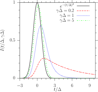
Figure 2: (color online) Time evolution of $I(t/\Delta,\gamma\Delta)$ for $\gamma\Delta=0.2$ (red), 1 (blue), and 5 (green). The Gaussian pulse is plotted as black curve.

III Third order optical nonlinearities

To illustrate how relaxation affects the third order optical nonlinearities, in the sample calculations presented below we assume equal relaxation rates for all orders of response, putting $\Gamma_{i}^{(n)}=\Gamma_{i}$ and $\Gamma_{e}^{(n)}=\Gamma_{e}$, and consider four sets of parameters: (a) $\Gamma_{i}=\Gamma_{e}=0$, (b) $\Gamma_{i}=\Gamma_{e}=33$ meV, (c) $\Gamma_{i}=65$ meV and $\Gamma_{e}=0.5$ meV, which are parameters used by Gu et al. Gu et al. (2012), (d) $\Gamma_{i}=0.5$ meV and $\Gamma_{e}=65$ meV. We define set (a) by the limit $\Gamma_{i}=\Gamma_{e}\to 0$, which recovers our relaxation free calculation Cheng et al. (2014a).

III.1 Third harmonic generation

For monochromatic incident light with frequency $\omega$, light is nonlinearly generated to lowest order at the third harmonic frequency $3\omega$ and at the fundamental frequency $\omega$. The first is described by the conductivity $\sigma^{(3);dabc}(\omega,\omega,\omega)$; the second corresponds to Kerr effects and two photon absorption, both described by $\sigma^{(3);dabc}(-\omega,\omega,\omega)$, and can be considered as a nonlinear correction to the linear optical response. In this section, we consider THG.

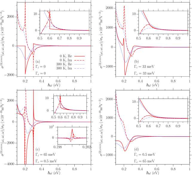
Figure 3: (color online) Spectra of $\sigma^{(3);xxxx}(\omega,\omega,\omega)$ at zero (thick red curves) and room (thin blue curves) temperatures for different relaxation parameters: (a) $\Gamma_{i}=\Gamma_{e}=0$, (b) $\Gamma_{i}=\Gamma_{e}=33$ meV, (c) $\Gamma_{i}=65$ meV and $\Gamma_{e}=0.5$ meV, (d) $\Gamma_{i}=0.5$ meV and $\Gamma_{e}=65$ meV. The real (imaginary) parts of the conductivity are given by the solid (dashed) curves; we have taken $|\mu|=0.3$ eV. The insets focus on results in the region $[0.5,1]$ eV. In (c) the fine structure in region $[0.198,0.202]$ eV is also displayed.

The conductivity tensor for THG only has one independent component

$$\sigma^{(3);xxyy}(\omega,\omega,\omega)=\sigma^{(3);xyxy}(\omega,\omega,\omega)$$ (49)

$$= \sigma^{(3);xyyx}(\omega,\omega,\omega)=\sigma^{(3);xxxx}(\omega,\omega,\omega)/3\,.$$

The induced current responsible for the THG is

$$\bm{J}^{(3);d}_{\text{THG}}(t)=e^{-i3\omega t}\sigma^{(3);xxxx}(\omega,\omega,\omega)\bm{E}_{\omega}\bm{E}_{\omega}\cdot\bm{E}_{\omega}+c.c\,.$$ (50)

In Fig. (3) we give the result for $\sigma^{(3);xxxx}(\omega,\omega,\omega)$ at $|\mu|=0.3$ eV for zero and room temperature. We first look at the results for zero temperature. The relaxation-free results are given as the thick (red) curves in Fig. 3 (a). This figure shows the step function of the real parts and the logarithmic divergence of the imaginary parts at three resonant photon energies $\hbar\omega=0.2$, $0.3$, and $0.6$ eV, which correspond to the resonant transitions for which the chemical potential gap $2|\mu|$ matches the energies of three photons, two photons, and one photon, respectively Cheng et al. (2014a). With relaxation included, the conductivity is a smooth function of $\omega$, and plotted in Fig. 3 (b), (c), and (d). Some common effects induced by the relaxations are shown: (i) the divergent peaks of the imaginary parts of the conductivity in Fig. 3 (a) become finite and broadened, (ii) the step functions of the real parts become continuous, (iii) the real parts become finite as $\hbar\omega<{2|\mu|}/{3}=0.2$ eV, and increase rapidly with decreasing frequency. They receive contributions not only from intraband transitions, describing Drude-like effects, but also from the interband transitions due to the linear dispersion relation of graphene (for example, see the prefactor $(\hbar\omega)^{-4}$ in Eq. (52)).

To illustrate the dominant features in these fine structures, we can analytically expand the coefficients of the functions ${\cal G}_{\mu}$, ${\cal H}_{\mu}$, ${\cal I}_{\mu}$, and the $|\mu|^{-1}$ term in the conductivity, for small relaxation parameters $\Gamma_{i,e}/(\hbar\omega)\ll 1$, to write

$$\sigma^{(3);xxyy}(\omega,\omega,\omega) = \sigma^{(3);xxyy}_{A}(\omega)+\sigma^{(3);xxyy}_{B}(\omega)$$ (51)

$$+ \sigma^{(3);xxyy}_{C}(\omega)\,,$$

with

$$\sigma^{(3);xxyy}_{A} (\omega)\approx\frac{i\sigma_{3}}{144(\hbar\omega)^{4}}\Big{[}17{\cal G}_{\mu}(\hbar\omega+i\Gamma_{e})$$ (52)

$$-64{\cal G}_{\mu}(2\hbar\omega+i\Gamma_{e})+45{\cal G}_{\mu}(3\hbar\omega+i\Gamma_{e})\Big{]}\,,$$

$$\sigma^{(3);xxyy}_{B} (\omega)\approx\frac{\Gamma_{i}}{\hbar}\frac{\sigma_{3}}{36(\hbar\omega)^{4}}\Big{[}-8{\cal H}_{\mu}(2\hbar\omega+i\Gamma_{e})$$

$$+17{\cal H}_{\mu}(3\hbar\omega+i\Gamma_{e})+3\omega{\cal I}_{\mu}(3\hbar\omega+i\Gamma_{e})\Big{]}\,,$$

$$\sigma^{(3);xxyy}_{C} (\omega)=-(\Gamma_{i}-\Gamma_{e})^{2}\dfrac{2i\sigma_{3}}{27(\hbar\omega)^{5}|\mu|}\,.$$

In the relaxation-free limit as $\Gamma_{e,i}\to 0$, $\sigma_{B}^{(3);xxyy}\to 0$ and $\sigma_{A}^{(3);xxyy}$ recovers the results of our previous work Cheng et al. (2014a). However, the relaxation-free limit of $\sigma_{C}^{(3);xxyy}$ strongly depends on the details of the chemical potential and relaxation parameters; this is the contribution to $\sigma_{C}^{(3);xxyy}$ from the general term discussed earlier in Eq. (31), which is problematic unless $\Gamma_{i}=\Gamma_{e}$. For doped graphene where $\mu$ is finite, $\sigma^{(3);xxyy}_{C}$ goes to zero with decreasing relaxation parameters; for graphene that is undoped or at low doping, a more sophisticated treatment is in order, as discussed in Section II.1. For the limit $\Gamma_{i,e},|\mu|\ll\hbar\omega$, the THG coefficient is approximated as

$$\sigma^{(3);xxyy}(\omega)\approx\dfrac{-i\sigma_{3}}{72(\hbar\omega)^{4}}\left[\pi+\frac{16(\Gamma_{i}-\Gamma_{e})^{2}}{3\hbar\omega|\mu|}\right]\,,$$ (53)

The term proportional to $\left|\mu\right|^{-1}$ did not arise in our previous calculation⁵, where we assumed that $\Gamma_{i,e}\rightarrow 0$ faster than $\mu\rightarrow 0$. Deferring the treatment of small doping to later studies, we focus here on graphene with large enough chemical potential that $\sigma_{C}^{(3);xxyy}(\omega)$ does not make a significant contribution to the full third harmonic conductivity.

At room temperature, the conductivities for different relaxation parameters look very similar to each other, and the fine structures caused by the resonant transitions are smeared out. This can be understood by the results in Appendix B: temperature affects the conductivity by smearing and lowering the peaks caused by functions ${\cal G}$, ${\cal H}$, and ${\cal I}$, which has an effect similar to increasing the value of $\Gamma_{e}$. If we increase each $\Gamma_{e}$ by the thermal energy of room temperature, the values of these new $\Gamma_{e}$ in the four cases presented in Fig. 3 are close, and it is not surprising that we get similar room temperature results.

III.2 Kerr effects and two photon absorption

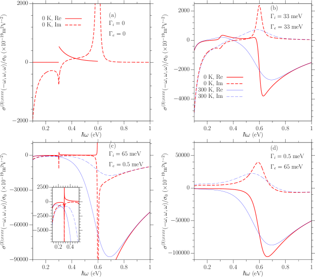
Figure 4: (color online) Spectra of $\sigma^{(3);xxxx}(-\omega,\omega,\omega)$ at zero (thick red curves) and room (thin blue curves) temperatures with different relaxation parameters: (a) $\Gamma_{i}=\Gamma_{e}=0$, (b) $\Gamma_{i}=\Gamma_{e}=33$ meV, (c) $\Gamma_{i}=65$ meV and $\Gamma_{e}=0.5$ meV, (d) $\Gamma_{i}=0.5$ meV and $\Gamma_{e}=65$ meV. The chemical potential is $|\mu|=0.3$ eV. The real (imaginary) parts of the conductivity are given by the solid (dashed) curves. The result in region $[0.1,0.55]$ eV of (c) is highlighted in the inset. In figure (a) the real part (solid curve) of $\sigma^{(3);xxxx}(-\omega,\omega,\omega)$ diverges for all $\hbar\omega>2\left|\mu\right|$.

We now turn to the light nonlinearity generated at the same frequency $\omega$ of the incident light. Taking $\bm{E}_{\omega}=\hat{\bm{x}}E_{\omega}^{x}+\hat{\bm{y}}E_{\omega}^{y}$, we write $\bm{E}_{\omega}=\begin{pmatrix}E_{\omega}^{x}\\ E_{\omega}^{y}\end{pmatrix}$ and consider

$$\bm{E}_{\omega}=E_{\omega}\begin{pmatrix}\cos\phi\\ \sin\phi e^{i\theta}\end{pmatrix}\,,\bm{E}_{-\omega}=E_{\omega}^{\ast}\begin{pmatrix}\cos\phi\\ \sin\phi e^{-i\theta}\end{pmatrix}\,.$$ (54)

The nonlinear response at frequency $\omega$ is then given by

$$\bm{J}^{(3)}(\omega) = 3E_{\omega}|E_{\omega}|^{2}\bigg{[}\sigma^{(3);xxxx}(\omega,\omega,-\omega)\begin{pmatrix}\cos\phi\\ \sin\phi e^{i\theta}\end{pmatrix}$$ (55)

$$+\sigma^{(3);xyyx}(\omega,\omega,-\omega)i\sin(2\phi)\sin\theta\begin{pmatrix}\sin\phi e^{i\theta}\\ -\cos\phi\end{pmatrix}\bigg{]}\,.\quad\quad$$

For linearly polarized light ($\theta=0$), the second term vanishes; the current from the first term has the same polarization as the incident field, and gives an intensity dependent correction of the linear conductivity $\sigma^{xx}_{\text{eff}}(\omega)=\sigma^{(1);xx}(\omega)+\sigma_{nl}(\omega)$, with

$$\sigma_{nl}(\omega)=3\sigma^{(3);xxxx}(\omega,\omega,-\omega)|E_{\omega}|^{2}\,.$$ (56)

An effective nonlinear susceptibility can be introduced Hendry et al. (2010); Kumar et al. (2013); Säynätjoki et al. (2013) $\chi_{nl}(\omega)=\sigma_{nl}(\omega)/(-i\omega\epsilon_{0}d_{\text{gr}})$, where the effective thickness of graphene single layer $d_{\text{gr}}$ is taken to be 3.3ÅHendry et al. (2010); from this an effective nonlinear refractive index $n_{2}$ and nonlinear loss $\beta_{\text{TPA}}$ can be extracted. In general, $\sigma^{(1);xx}$ has both real part and imaginary parts, and the calculation of $n_{2}$ and $\beta_{\text{TPA}}$ should follow the results of del Corso and Soles [del Coso and Solis, 2004].

In the limit of no relaxation, we showed earlier Cheng et al. (2014a) that $\sigma^{(3);dabc}(-\omega,\omega,\omega)$ has many divergences, and its behavior in the neighborhood of equal frequencies can be written as

$$\sigma^{(3);dabc}(-\omega,\omega+\delta_{1},\omega+\delta_{2})$$ (57)

$$= \frac{{\cal T}_{1}^{dabc}(\omega)}{\delta_{1}\delta_{2}}+\frac{{\cal T}_{2}^{dabc}(\omega;\delta_{2})}{\delta_{1}}+\frac{{\cal T}_{2}^{dabc}(\omega;\delta_{1})}{\delta_{2}}$$

$$+{\cal T}_{3}^{dabc}(\omega;\delta_{1},\delta_{2})\,,$$

where ${\cal T}_{1}^{dabc}$, ${\cal T}_{2}^{dabc}$, and ${\cal T}_{3}^{dabc}$ are all smooth functions of $\delta_{1}$ and $\delta_{2}$. The strength of the singularities is determined by ${\cal T}_{1}^{dabc}$ and ${\cal T}_{2}^{dabc}$, which are real functions and are only nonzero when the photon energy is greater than that for the onset of one-photon absorption ($\hbar\omega>2|\mu|$). For fixed photon energy $\hbar\omega$, the appearance of the divergence as $\mu$ decreases from $2|\mu|>\hbar\omega$ to $2|\mu|\leq\hbar\omega$ indicates that it is associated with the existence of electrons (holes) at the $\bm{k}$ where one-photon absorption is possible. Physically, at these $\bm{k}$ the third order correction to one-photon absorption would lead to the perturbative description of the saturation, but in the absence of relaxation that correction diverges, as it would for an inhomogeneously broadened collection of two-level systems. At zero temperature, the sharp Fermi surface can strictly exclude such electrons (holes) for $2|\mu|>\hbar\omega$. However, at finite temperature thermal fluctuations will always place some electrons (holes) at $\bm{k}$ where one-photon absorption can occur, and so the divergence in the third order response will exist for any photon energy.

Including relaxation parameters $\Gamma_{i}^{(j)}=\Gamma_{i}$ and $\Gamma_{e}^{(j)}=\Gamma_{e}$, $\sigma^{(3);dabc}(-\omega,\omega+\delta_{1},\omega+\delta_{2})$ includes terms that are proportional to $t_{1}=(\delta_{1}+i\Gamma_{i})^{-1}$, $t_{2}=(\delta_{2}+i\Gamma_{i})^{-1}$, $t_{a}=(\delta_{1}+\delta_{2}+2i\Gamma_{e})^{-1}$, $t_{1}t_{a}$, and $t_{2}t_{a}$. As any of these three quantities $\delta_{1}+i\Gamma_{i}$, $\delta_{2}+i\Gamma_{i}$, or $\delta_{1}+\delta_{2}+2i\Gamma_{e}$ goes to zero, $\sigma^{(3);dabc}(-\omega,\omega,\omega)$ diverges. But for nonzero $\Gamma_{i}$ and $\Gamma_{e}$, $\sigma^{(3);dabc}(-\omega,\omega+\delta_{1},\omega+\delta_{2})$ is a smooth function of real $\omega$, $\delta_{1}$, and $\delta_{2}$. For a pulse response when the energy broadening of the pulse is less than the relaxation energies, it is reasonable to set $\delta_{1}=\delta_{2}=0$, and then the conductivity can be written as

$$\sigma^{(3);dabc}(-\omega,\omega,\omega) = \frac{{\cal L}_{1}^{dabc}(\omega)}{\Gamma_{i}\Gamma_{e}}+\frac{{\cal L}^{dabc}_{2}(\omega;\Gamma_{e})}{\Gamma_{i}}$$ (58)

$$+\frac{{\cal L}^{dabc}_{3}(\omega;\Gamma_{i},\Gamma_{e})}{\Gamma_{e}}$$

$$+{\cal L}^{dabc}_{4}(\omega;\Gamma_{i},\Gamma_{e})\,,$$

with

$${\cal L}_{1}^{dabc}(\omega) = i\sigma_{3}\frac{A_{0}}{12(\hbar\omega)^{2}}\left[{\cal G}_{\mu}(\vartheta_{+})+{\cal G}_{\mu}(\vartheta_{-})\right]\,,$$ (59)

$${\cal L}_{2}^{dabc}(\omega;\Gamma_{e}) = \frac{\sigma_{3}A_{0}}{12(\hbar\omega)^{2}}\left\{\frac{\vartheta_{+}}{\vartheta_{-}^{2}}{\cal G}_{\mu}(\vartheta_{-})\right.$$ (60)

$$+\frac{5\vartheta_{+}^{2}-3\theta_{-}^{2}}{2\vartheta_{+}^{3}}{\cal G}_{\mu}(\vartheta_{+})$$

$$\left.+\frac{2\hbar\omega}{\vartheta_{+}^{2}}\left[\hbar\omega{\cal H}_{\mu}(\vartheta_{+})+\frac{4\Gamma_{e}^{2}}{\vartheta_{-}|\mu|}\right]\right\}\,,$$

$${\cal L}_{3}^{dabc} (\omega;\Gamma_{i},\Gamma_{e})=\frac{\sigma_{3}\Gamma_{i}}{6(\hbar\omega)^{2}\nu_{+}}\Big{\{}i(A_{0}-A_{1}){\cal G}_{\mu}(i\Gamma_{e})$$ (61)

$$-\frac{\Gamma_{i}\Gamma_{e}}{|\mu|(4\mu^{2}+\Gamma_{e}^{2})\nu_{+}}\left(A_{1}+A_{0}+\frac{2\nu_{+}}{\nu_{-}}A_{1}\right)\Big{\}}\,,$$

The full expression of ${\cal L}_{4}^{dabc}(\omega;\Gamma_{i},\Gamma_{e})$ is complicated; we can achieve a good approximation by setting $\Gamma_{i}=0$, for which

$${\cal L}_{4}^{dabc}(\omega;0,\Gamma_{e})$$ (62)

$$= \frac{i\sigma_{3}}{12(\hbar\omega)^{4}}\Big{\{}2(A_{1}-A_{0}){\cal G}_{\mu}(i\Gamma_{e})+4(3A_{1}+A_{0}){\cal G}_{\mu}(\vartheta_{+})$$

$$-(4A_{1}+5A_{0}){\cal G}_{\mu}(\vartheta_{-})-8(A_{1}+A_{0}){\cal G}_{\mu}(2\hbar\omega+i\Gamma_{e})$$

$$-\frac{4\mu(\hbar\omega)^{2}}{(\vartheta_{+}^{2}-4\mu^{2})^{2}}\left[(A_{1}+4A_{0})\vartheta_{+}+A_{0}\frac{\vartheta_{+}^{2}-4\mu^{2}}{\hbar\omega}\right]\Big{\}}\,.\quad\quad$$

In these expressions, we used $\vartheta_{\pm}=\pm\hbar\omega+i\Gamma_{e}$ and $\nu_{\pm}=\pm\hbar\omega+i\Gamma_{i}$.

In Fig. 4, the photon energy dependence of $\sigma^{(3);dabc}(-\omega,\omega,\omega)$ is plotted for different relaxation parameters, with chemical potential $|\mu|=0.3$ eV at zero and room temperatures. Fig. 4 (a) gives the relaxation-free calculation, which is done as $\lim\limits_{\Gamma_{i}=\Gamma_{e}\to 0}\sigma^{(3);dabc}(-\omega,\omega,\omega)$. Three regimes are apparent: (1) $\hbar\omega<|\mu|$, in which both one- and two- photon absorption are absent, and the real part of the conductivity is zero. The imaginary part at low photon energy scales as $(\hbar\omega)^{-3}$. At $\hbar\omega=|\mu|$, the real part shows a step function, while the imaginary part shows a logarithmic divergence. (2) $|\mu|<\hbar\omega<2|\mu|$, in which two-photon absorption is present but one-photon absorption is still absent. The real part of the conductivity here scales as $(\hbar\omega)^{-4}$. Around $\hbar\omega=2|\mu|$, the imaginary part shows a divergence $(\hbar\omega-2|\mu|)^{-2}$. For frequencies satisfying $\hbar\omega<2|\mu|$, if the graphene is subject to a Gaussian pulse sufficiently narrow in frequency, the nonlinear current induced will still have a shape that is approximately Gaussian, and characterizing the nonlinear response to a pulse by Eq. (56) makes sense. (3) $\hbar\omega>2|\mu|$, where both two- and one-photon absorption are present. The imaginary part of the conductivity diverges as $(\hbar\omega-2|\mu|)^{-2}$ around $\hbar\omega=2|\mu|$, and the real part diverges for the entire region $\hbar\omega>2|\mu|$. At finite temperature and in the absence of relaxation, the real part diverges for any photon energy $\hbar\omega$. As we discussed after Eq. (57), the divergence of the real part of $\sigma^{(3);dabc}(-\omega,\omega,\omega)$ is induced by the existence of electrons (holes) at the $\bm{k}$ where one-photon absorption occurs; at zero temperature, these electrons (holes) only exist when the chemical potential $|\mu|<\hbar\omega/2$, while at finite temperature, they exist at any chemical potential due to thermal fluctuations.

In Fig. 4 (b), (c), and (d), we present the results for the same relaxation parameters as those adopted in the THG calculation. Relaxation affects the conductivity in a complex way, but there are some qualitative features that can be identified: (i) In the neighborhood of the divergences that arise in the relaxation-free calculation, including the divergent regime $\hbar\omega>2\left|\mu\right|$ and the special frequency $\hbar\omega=\left|\mu\right|$, both the real and imaginary parts of the conductivity are lowered and are everywhere finite. In Fig. 4 (b), (c), and (d), we find that a larger $\Gamma_{e}$ gives lower and broader peaks at $\hbar\omega=|\mu|$ and $2|\mu|$. (ii) For the relaxation parameters used here, the real part of the conductivity is negative for $\hbar\omega>2|\mu|$. Because of the presence in this frequency range of one-photon absorption, which is always positive, the two-photon absorption processes indicated by the real part of $\sigma^{(3);dabc}(-\omega,\omega,\omega)$ can be understood as a correction to the simple linear prediction of the absorption. In fact, we can find a range of electric fields large enough so that $\sigma^{da}_{\text{eff}}(\omega)$ is negative; for a field anywhere near or above this strength the perturbative result is naturally suspect. (iii) Even for frequencies in the range $\left|\mu\right|<\hbar\omega<2\left|\mu\right|$, where only two-photon absorption is present in the absence of relaxation, the real part of the nonlinear conductivity $\sigma^{(3);dabc}(-\omega,\omega,\omega)$ can be negative. Yet in the presence of relaxation the linear conductivity $\sigma^{(1);xx}(\omega)$ acquires a real part in this frequency range, and the real part of $\sigma_{\text{eff}}^{xx}(\omega)$, for example, is always positive for small enough electric field amplitudes, indicating absorption. However, these results indicate the sensitivity to the relaxation parameters of both the third order conductivity, and its interplay with the first order conductivity, and a more sophisticated description of the scattering is clearly in order.

At room temperature, the peaks or divergences are further broadened. For a given frequency $\omega$, the regime $\hbar\omega>2|\mu|$ always contributes to a finite temperature calculation due to the average over the chemical potential. The absolute values of the real part of the conductivity in the regime $\hbar\omega<2|\mu|$ also significantly increase.

III.3 Two-color coherent current injection

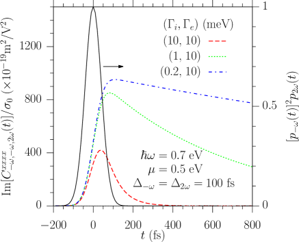
Figure 5: (color online) Time evolution of $\text{Im}[C^{xxxx}_{-\omega,-\omega,2\omega}(t)]$ for Gaussian pulses with $\Delta_{-\omega}=\Delta_{2\omega}=100$ fs for different relaxation parameters $(\Gamma_{i},\Gamma_{e})=(0.2,10)$ meV (blue chain curve), $(1.0,10)$ meV (green dotted curve), and $(10,10)$ meV (red dashed curve), $(10,1)$ meV, and $(10,0.2)$ meV. The last three cases overlap with the red dashed curve. The pulse width corresponds to an energy broadening $\hbar\Delta_{-\omega}=6.6$ meV. Our calculations show $\text{Re}[C^{xxxx}_{-\omega,-\omega,2\omega}(t)]$ is negligible on this scale.

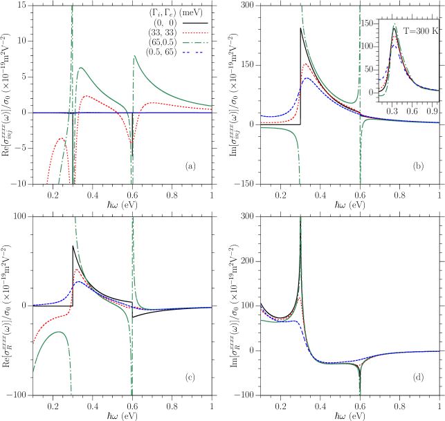
Figure 6: (color online) Spectra of $\sigma_{inj}^{xxxx}(\omega)$ (a, b) and $\sigma_{R}^{xxxx}(\omega)$ (c, d) for different relaxation parameters $\Gamma_{i}$ and $\Gamma_{e}$ at temperature $T=0$: Black solid curves: $\Gamma_{i}=\Gamma_{e}=0$; Red dotted curves: $\Gamma_{i}=\Gamma_{e}=33$ meV; green chain curves: $\Gamma_{i}=65$ meV, $\Gamma_{e}=0.5$ meV; Blue dashed curves: $\Gamma_{i}=0.5$ meV, $\Gamma_{e}=65$ meV. The chemical potential is $|\mu|=0.3$ eV. The result of $\text{Im}[\sigma_{inj}^{xxxx}(\omega)]$ at 300 K is shown in the inset of (b).

Now we turn to two-color coherent current injection, with frequencies $\omega_{1}=\omega_{2}=-\omega$ and $\omega_{3}=2\omega$. In the relaxation-free calculation, the conductivity $\sigma^{(3);dabc}(-\omega,-\omega,2\omega)$ diverges, and it is the divergence that describes the current injection. In fact, in the neighborhood of these frequencies, the conductivity can be written as

$$\sigma^{(3);dabc}(-\omega,-\omega,2\omega+\delta\omega)=\frac{i\eta^{dabc}(\omega)}{3\delta\omega}+\sigma^{(3);dabc}_{R}(\omega)\,,$$ (63)

where the injected current is determined by a well-behaved function $\eta^{dabc}(\omega)$, and $\sigma^{(3);dabc}_{R}(\omega)$ is a smooth function of $\delta\omega$. With the inclusion of relaxation, the conductivity $\sigma^{(3);dabc}(-\omega,-\omega,2\omega)$ itself is well behaved. The divergence term in the relaxation-free limit becomes a term similar to the right hand side of Eq. (45). To check whether $\Gamma_{i}$ and $\Gamma_{e}$ have the same importance for the injection, we give the pulse calculations of $C^{xxxx}_{-\omega,-\omega,2\omega}(t)$ (see Eq. 39) in Fig. 5 for different relaxation parameters. After the laser pulse, the current response persists for times associated with $\Gamma_{i}$, showing that the contribution from $\Gamma_{i}$ dominates the relaxation of the injected current, as might be expected. To highlight this, we write

$$\sigma^{(3);dabc}(-\omega+\delta_{1},-\omega+\delta_{2},2\omega+\delta_{3})$$ (64)

$$= \frac{i\eta^{dabc}(\omega)}{3(\delta_{1}+\delta_{2}+\delta_{3}+i\hbar^{-1}\Gamma_{i})}+\sigma^{(3);dabc}_{R}(\omega)\,,$$

From Eq. (15), only terms ${\cal S}_{1-4}^{dabc}$ including $(\delta_{1}+\delta_{2}+\delta_{3}+i\Gamma_{i})^{-1}$ contribute to $\eta^{dabc}(\omega)$. By writing $\sigma_{inj}^{dabc}(\omega)\equiv{\hbar\eta^{dabc}(\omega)}/{\text{1eV}}$, the first term in Eq. (64) becomes

$$\frac{1\text{eV}}{3(\hbar\delta_{1}+\hbar\delta_{2}+\hbar\delta_{3}+i\Gamma_{i})}i\sigma_{inj}^{dabc}(\omega)$$ (65)

with

$$\sigma_{inj}^{dabc}(\omega) \approx \frac{i\sigma_{3}}{\text{1eV}}\Bigg{\{}-\frac{2A_{3}+A_{0}}{2(\hbar\omega)^{3}}\text{Im}[{\cal G}_{\mu}(\hbar\omega+i\Gamma_{e})]$$ (66)

$$+\frac{A_{3}+A_{0}}{(\hbar\omega)^{3}}\text{Im}[{\cal G}_{\mu}(2\hbar\omega+i\Gamma_{e})]$$

$$+\frac{6\Gamma_{e}A_{3}+5\Gamma_{i}A_{0}}{4(\hbar\omega)^{4}}\text{Re}[{\cal G}_{\mu}(\hbar\omega+i\Gamma_{e})]$$

$$-\frac{3\Gamma_{e}(A_{0}+A_{3})+\Gamma_{i}A_{0}}{4(\hbar\omega)^{4}}\text{Re}[{\cal G}_{\mu}(2\hbar\omega+i\Gamma_{e})]$$

$$-\frac{\Gamma_{i}(A_{3}+A_{0})}{4(\hbar\omega)^{3}}{\cal H}_{\mu}(-2\hbar\omega+i\Gamma_{e})$$

$$+\frac{\Gamma_{i}(A_{3}+2A_{0})}{4(\hbar\omega)^{3}}{\cal H}_{\mu}(\hbar\omega+i\Gamma_{e})\Bigg{\}}\,,$$

where terms proportional to $|\mu|^{-1}$ are neglected. As $\Gamma_{i},\Gamma_{e}\to 0$, only terms involving $\text{Im}[{\cal G}_{\mu}(\omega)]\propto\theta(|\omega|-2|\mu|)$ remain; $\sigma^{dabc}_{inj}(\omega)$ is a pure imaginary quantity, and is consistent with our previous work Cheng et al. (2014a). With relaxation included, terms involving $\text{Re}[{\cal G}_{\mu}]$ and ${\cal H}_{\mu}$ appear.

In Fig. 6 (a) and (b) we plot the photon energy dependence of $\sigma_{inj}^{xxxx}(\omega)$ for different relaxation parameters at zero and room temperature. The real part is much smaller than the imaginary part. At zero temperature, we see in Fig. 6 (b) that for $\Gamma_{e}=0.5$ meV there are fine structures in the spectrum of $\text{Im}[\sigma^{xxxx}_{inj}(\omega)]$ around $\hbar\omega=|\mu|$ and $\hbar\omega=2|\mu|$; it is due to the ${\cal H}_{\mu}$ terms. As can be seen in the inset of Fig. 6 (b), finite temperature and finite $\Gamma_{e}$ lead to similar broadening and lowering of the peaks.

We also plot $\sigma^{xxxx}_{R}(\omega)$ in Fig. 6 (c) and (d). The amplitude of $\sigma^{xxxx}_{R}$ is of the same order of magnitude as that of $\sigma^{xxxx}_{inj}$. However, due to the prefactor $1\text{eV}/(3\Gamma_{i})$, which relates $\sigma_{inj}^{xxxx}$ to its contribution to $\sigma^{(3);dabc}(-\omega,-\omega,2\omega)$ in Eq. (65), $\sigma^{xxxx}_{inj}$ dominates for small $\Gamma_{i}$, usually taken to be a few tens of meV.

III.4 Parametric frequency conversion

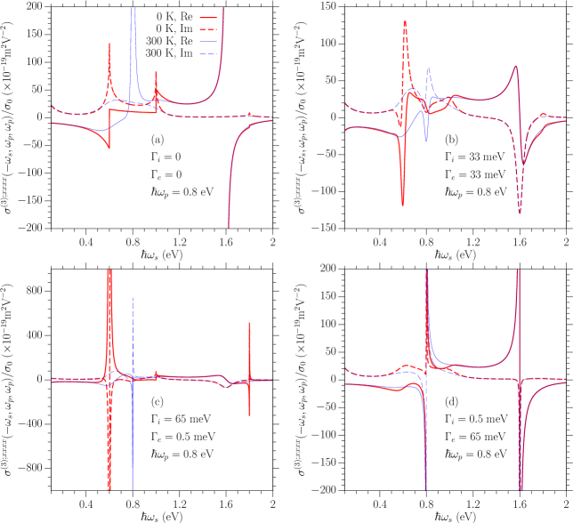
Figure 7: (color online) Spectra of $\sigma^{(3);xxxx}(-\omega_{s},\omega_{p},\omega_{p})$ for different relaxation parameters at zero (thick red curves) and room temperature (thin blue curves). Solid (dashed) curves give their real (imaginary) parts separately. In the calculation, the chemical potential is $|\mu|=0.5$ eV, and the pump photon energy is $\hbar\omega_{p}=0.8$ eV.

Third order nonlinearities can lead to the appearance of new frequencies via parametric frequency conversion, which is described by $\sigma^{(3);dabc}(-\omega_{s},\omega_{p},\omega_{p})$. Here $\omega_{p}$ is the frequency of a strong pump field, and $\omega_{s}$ is the signal frequency converted by interaction with the pump to an idler frequency $\omega_{i}=2\omega_{p}-\omega_{s}$. Possible resonant transitions occur as any of the frequencies $|\omega_{p}|$, $|\omega_{s}|$, $|\omega_{p}-\omega_{s}|$, $|2\omega_{p}|$, or $|2\omega_{p}-\omega_{s}|$ equal $2|\mu|/\hbar$. In Fig. 7 we plot the dependence of $\sigma^{(3);xxxx}(-\omega_{s},\omega_{p},\omega_{p})$ on $\omega_{s}$ for different relaxation parameters at $\hbar\omega_{p}=0.8$ eV and $|\mu|=0.5$ eV.

At zero temperature, the calculations show peaks/step functions for resonant transitions at $\hbar\omega_{s1}=2\hbar\omega_{p}-2|\mu|=0.6$ eV, $\hbar\omega_{s2}=2|\mu|=1.0$ eV, or $\hbar\omega_{s3}=2|\mu|+\hbar\omega_{p}=1.8$ eV, both with and without the inclusion of relaxation. Around these resonant transitions, the behavior of the conductivity can be analyzed as following:

(1) Around $\omega_{s}=\omega_{s1}+\delta\omega$, the idler photon energy $\hbar\omega_{i}=2|\mu|-\hbar\delta\omega$ is close to the onset of the one-photon absorption. By taking $\vartheta=\hbar\omega_{i}+i\Gamma_{e}=2|\mu|-\hbar\delta\omega+i\Gamma_{e}$, the conductivity as $\delta\omega\to 0$ is determined by functions ${\cal G}_{\mu}(\vartheta)\sim\ln(\hbar\delta\omega-i\Gamma_{e})$, ${\cal H}_{\mu}(\vartheta)\sim(\hbar\delta\omega-i\Gamma_{e})^{-1}\Gamma_{i}$, and ${\cal I}_{\mu}(\vartheta)\sim(\hbar\delta\omega-i\Gamma_{e})^{-2}\Gamma_{i}$. In the relaxation-free limit, only ${\cal G}_{\mu}(\vartheta)$ contributes a logarithmic divergence to the imaginary part, and a step change in the real part [in Fig. 7 (a)] for nonzero $\delta\omega$. With the inclusion of relaxation, we can distinguish three different types of qualitative behavior, shown in Fig. 7 (b) - (d), based on the relative magnitude of $\Gamma_{i}$ and $\Gamma_{e}$: (b) $\Gamma_{i}=\Gamma_{e}$, all functions contribute; (c) $\Gamma_{e}\ll\Gamma_{i}$, ${\cal I}_{\mu}(\vartheta)$ dominates; (d) $\Gamma_{e}\gg\Gamma_{i}$, where for the values chosen the relaxation is large enough to smear out these resonances.

(2) Around $\omega_{s}=\omega_{s2}+\delta\omega$, the signal frequency is close to the onset of the one-photon absorption. For non-resonant transitions in a usual semiconductor, $\omega_{s_{2}}$ and $\omega_{s_{1}}$ are interchangeable frequencies to give the same conductivity of parametric frequency conversion Boyd (2008); here in graphene they yield asymmetric peaks because the resonant transitions dominate. In the limit of no relaxation, the conductivity shows a logarithmic divergence that is easily smeared out by the inclusion of small relaxation parameters.

(3) Around $\omega_{s}=\omega_{s3}+\delta\omega$: By taking $\vartheta=-\hbar\omega_{s}+\hbar\omega_{p}+i\Gamma_{e}=-2|\mu|-\hbar\delta\omega+i\Gamma_{e}$, the conductivity as $\delta\omega\to 0$ is determined by functions ${\cal G}_{\mu}(\vartheta)\sim\ln(\hbar\delta\omega-i\Gamma_{e})$ and ${\cal H}_{\mu}(\vartheta)\sim(\hbar\delta\omega-i\Gamma_{e})^{-1}\Gamma_{i}$. In the limit of no relaxation, ${\cal G}_{\mu}$ gives a small peak. For $\Gamma_{e}\ll\Gamma_{i}$, the peak from ${\cal H}_{\mu}$ is stronger but very narrow.

(4) At finite temperature there is a further smearing of the peaks around the resonances, as described in Appendix B.

Besides these resonant transitions, two singularities are apparent: (i) the singularity around $\omega_{s}=2\omega_{p}$, which corresponds to two-color coherent current injection. The singularity is not determined by the behavior of the functions ${\cal G}$, ${\cal H}$, ${\cal I}$, but by the coefficients that premultiply them in Eqs. (19) to (26). Around $\omega_{s}=2\omega_{p}$ we put $\omega_{s}=2\omega_{p}+\delta\omega$ and find

$$\sigma^{(3);xxxx}(-2\omega_{p}+\delta\omega,\omega_{p},\omega_{p})$$

$$= \frac{1\text{eV}}{\hbar\delta\omega+i\Gamma_{i}}i\sigma^{(3);xxxx}_{inj}(\omega_{p})+\sigma^{(3);xxxx}_{R}(\omega_{p})\,,$$

an equation similar to Eq. (64) discussed in Section III.3. Two-color coherent current injection requires both one-photon absorption (for $\omega_{s}$) and two photon absorption (for $\omega_{p}$), i.e., $\hbar\omega_{p}>|\mu|$. The parameters we have adopted in Fig. 7 fulfill this criterion, and thus the singularity appears. Finite temperatures do not qualitatively affect this singularity because it is not related to the chemical potential. (ii) The strong response around $\omega_{s}=\omega_{p}$ is related to the third order correction to one-photon absorption, and only appears at finite temperature. Since $|\mu|<\hbar\omega_{p}<2|\mu|$, at zero temperature only two-photon absorption is present and there is no one-photon absorption. However, at finite temperature thermal fluctuations will place electrons where one-photon absorption can occur, and the third order correction to that will lead, in the absence of relaxation, to a divergent result as discussed in Section III.2; in the presence of relaxation the result will not be divergent but very large, describing the saturation of the one-photon absorption at the level of the third order response.

III.5 Comparison between calculations and experiments

Experiments have already extracted values of the effective third order susceptibilities of THG Kumar et al. (2013); Säynätjoki et al. (2013); Hong et al. (2013), two-photon absorption Zhang et al. (2012); Hong et al. (2013), Kerr effects Yang et al. (2011); Gu et al. (2012); Wu et al. (2011), and parameter frequency conversion Hendry et al. (2010) at some photon energies. The nonlinear conductivities we have calculated here are related to the effective susceptibility by Hendry et al. (2010); Cheng et al. (2014a)

$$\chi^{(3);dabc}_{\text{eff}}(\omega_{1},\omega_{2},\omega_{3})=\frac{\sigma^{(3);dabc}(\omega_{1},\omega_{2},\omega_{3})}{-i(\omega_{1}+\omega_{2}+\omega_{3})\epsilon_{0}d_{\text{gr}}}\,.$$ (67)

We first look at the THG, for which the experimental technique is perhaps the most mature, and the extracted values can likely be considered more reliable than those from other effects. For a reasonable chemical potential estimated from the sample preparation, the calculations without relaxation parameters Cheng et al. (2014a) yield theoretical results for the nonlinear conductivity about two orders of magnitude smaller than the value extracted from experiments. Here we have found that calculations at finite temperature for different sets of relaxation parameters (see the insets of Fig. 3) are almost the same as calculations at zero temperature and neglecting relaxation.

For Kerr effects, because of the existence of divergent terms in the expressions and the probably very low chemical potential in experiments, it is not surprising that we could fit the nonlinear susceptibility at one photon energy by tuning the relaxation parameters. The complicated dependence is shown in Fig. 4. As $\hbar\omega>2|\mu|$, the nonlinear conductivity at both zero and room temperatures can vary many orders of magnitude, depending on the relaxation parameters adopted.

For parametric frequency conversion observed in the experiment by Hendry et al. Hendry et al. (2010), with parameters $\hbar\omega_{p}=1.31$ eV, $\hbar\omega_{s}=1.05$ eV, and assuming a low chemical potential $|\mu|=0.1$ eV, we checked the dependence of the conductivity on the relaxation parameters $\Gamma_{i}$ and $\Gamma_{e}$ in the range of $[0,60]$ meV. We find the dependence is weak and the calculated values are still smaller than their claimed values by two orders of magnitude Hendry et al. (2010).

Admittedly the measured effective susceptibilities for parametric frequency conversion, Kerr effects and two photon absorption, and THG show a strong dependence on the measurement method, light frequency, pulse duration, and perhaps sample preparation. Yet even taking this into account, the conclusion that the theoretical results are about two orders of magnitude smaller than the measured results is inescapable. These discrepancies could arise for a number of reasons, including: (1) The samples in many experiments are not suspended graphene, but graphene on a substrate or in solution. Thus there may have been contributions to the optical nonlinearity from the interaction between the graphene sheet and its environment, which may be crucial considering that graphene is a one-atom thick material. (2) Thermal effects Boyd (2008) caused by a high repetition rate of laser pulses, as used in $Z$-scan experiments, may play an important role Liu et al. (2011b); Zhang et al. (2013). (3) Because of the zero gap of graphene and the intense laser beams used in experiments, saturation Bao et al. (2009) induced by one and/or two photon absorption can make necessary a treatment more sophisticated than that of perturbation theory. Zhang et al. Zhang and Voss (2011) used the density matrix method to study four wave mixing in undoped graphene in the saturation regime, and found an effective $\chi^{(3)}_{\text{eff}}$ about $10^{-17}$ m²/V², and decreasing with increasing light intensity. Additional calculations for different third-order nonlinear effects in graphene in the saturation regime are needed to assess the impact of saturation on the theoretical nonlinearities. (4) The calculation at the independent particle level, which works well as a starting point for most gapped semiconductors, may fail in graphene, and it may be necessary to do a more realistic calculation, including the full band structure, and the detailed effects of scattering and the electron-electron interactions.

IV DC current induced second order nonlinearity

unsymmetrized $\widetilde{\sigma}$	relaxation parameters	unsymmetrized $\widetilde{\sigma}$	relaxation parameters
	$\Gamma_{i}^{(3)}=\Gamma_{i}^{\text{dc}}$	$\widetilde{\sigma}^{(3);dacb}(\omega_{1},0,\omega_{2})$
$\widetilde{\sigma}^{(3);dabc}(\omega_{1},\omega_{2},0)$	$\Gamma_{e}^{(3)}=\Gamma_{e}^{\text{dc}}$	$\widetilde{\sigma}^{(3);dbca}(\omega_{1},0,\omega_{2})$	$\Gamma_{i}^{(j)}=\Gamma_{i}^{\text{op}}$
$\widetilde{\sigma}^{(3);dbac}(\omega_{2},\omega_{1},0)$	$\Gamma_{i}^{(1,2)}=\Gamma_{i}^{\text{op}}$	$\widetilde{\sigma}^{(3);dcab}(0,\omega_{1},\omega_{2})$	$\Gamma_{e}^{(j)}=\Gamma_{e}^{\text{op}}$
	$\Gamma_{e}^{(1,2)}=\Gamma_{e}^{\text{op}}$	$\widetilde{\sigma}^{(3);dcba}(0,\omega_{2},\omega_{1})$

Table 1: Relaxation parameters used in the different processes associated with the dc current induced second order nonlinearity.

We now turn to the limiting case where one of the electric fields is a dc field, taking $\omega_{3}=0$. The calculation of $\widetilde{\sigma}^{(3);dabc}(\omega_{1},\omega_{2},0)$ from Eq. (15) includes a term proportional to

$$\dfrac{1}{\hbar\omega_{3}+i\Gamma_{i}^{(3)}}\rightarrow\dfrac{1}{i\Gamma_{i}^{(3)}}\,.$$ (68)

Therefore a nonzero relaxation $\Gamma_{i}^{(3)}$ for the dc field is necessary to set up a steady state with a dc charge current in graphene. For other transitions included in $\widetilde{\sigma}^{(3);dacb}(\omega_{1},0,\omega_{2})$ and $\widetilde{\sigma}^{(3);dcab}(0,\omega_{1},\omega_{2})$, it is not necessary to include relaxation associated with the dc field, because the dc field acts on the optical excitation with frequency $\omega_{2}$ and $\omega_{1}+\omega_{2}$ respectively; these only survive during the optical pulse. We list the relaxation parameters used in calculating the unsymmetrized conductivities in Table 1. The third order conductivity of interest here, which we can refer to as the dc-induced second order optical conductivity, can be written as

$$\sigma^{(3);dabc}(\omega_{1},\omega_{2},0)=\frac{1\text{eV}}{3\Gamma_{i}^{\text{dc}}}\sigma_{J}^{dabc}(\omega_{1},\omega_{2})+\sigma_{E}^{dabc}(\omega_{1},\omega_{2})\,.$$ (69)

The first term includes all contributions that diverge as $1/\Gamma_{i}^{\text{dc}}$, which are only involved in calculating $\widetilde{\sigma}^{(3);dabc}(\omega_{1},\omega_{2},0)$ and $\widetilde{\sigma}^{(3);dbac}(\omega_{2},\omega_{1},0)$; they both occur with the dc charge current. Thus we can associate it with the dc current-induced second order conductivity, in that it is second order in the optical fields at $\omega_{1}$ and $\omega_{2}$. The second term includes all other contributions, and we can associate it with a dc field-induced second order conductivity, which exists even for a gapped semiconductor without doping. Examining Eq. (15), we see that $\sigma_{J}^{dabc}(\omega_{1},\omega_{2})$ is independent of $\Gamma_{i}^{\text{dc}}$ and $\Gamma_{e}^{\text{dc}}$, and it can be written as

$$\sigma_{J}^{dabc}(\omega_{1},\omega_{2})=\frac{i\sigma_{3}}{\text{1eV}}S_{J}^{dabc}(\omega_{1},\omega_{2})$$

with

$$S_{J}^{dabc}(\omega_{1},\omega_{2}) = \left[\frac{A_{1}}{(\hbar\omega_{2})^{2}}+\frac{A_{3}}{\hbar\omega_{1}+i\Gamma_{e}^{\text{op}}}\left(\frac{1}{\hbar\omega_{1}+\hbar\omega_{2}+i\Gamma_{i}^{\text{op}}}-\frac{1}{\hbar\omega_{2}}\right)\right]{\cal H}_{\mu}(\hbar\omega_{1}+i\Gamma_{e}^{\text{op}})$$ (70)

$$+ \left[\frac{A_{2}}{(\hbar\omega_{1})^{2}}+\frac{A_{3}}{\hbar\omega_{2}+i\Gamma_{e}^{\text{op}}}\left(\frac{1}{\hbar\omega_{1}+\hbar\omega_{2}+i\Gamma_{i}^{\text{op}}}-\frac{1}{\hbar\omega_{1}}\right)\right]{\cal H}_{\mu}(\hbar\omega_{2}+i\Gamma_{e}^{\text{op}})$$

$$+ \left[-\frac{A_{1}}{(\hbar\omega_{2})^{2}}-\frac{A_{2}}{(\hbar\omega_{1})^{2}}-\frac{A_{1}+A_{2}+A_{3}}{\hbar\omega_{1}+\hbar\omega_{2}+i\Gamma_{e}^{\text{op}}}\left(\frac{1}{\hbar\omega_{1}+i\Gamma_{i}^{\text{op}}}+\frac{1}{\hbar\omega_{2}+i\Gamma_{i}^{\text{op}}}\right)\right.$$

$$\left.+\frac{A_{3}}{\hbar\omega_{1}+\hbar\omega_{2}+i\Gamma_{e}^{\text{op}}}\left(\frac{1}{\hbar\omega_{1}}+\frac{1}{\hbar\omega_{2}}\right)\right]{\cal H}_{\mu}(\hbar\omega_{1}+\hbar\omega_{2}+i\Gamma_{e}^{\text{op}})$$

$$+ \left[\left(\frac{1}{\hbar\omega_{2}+i\Gamma_{i}^{\text{op}}}-\frac{1}{\hbar\omega_{2}}\right)A_{1}+\left(\frac{1}{\hbar\omega_{1}+i\Gamma_{i}^{\text{op}}}-\frac{1}{\hbar\omega_{1}}\right)A_{2}\right]{\cal I}_{\mu}(\hbar\omega_{1}+\hbar\omega_{2}+i\Gamma_{e}^{\text{op}})$$

$$+ \left(\frac{1}{\hbar\omega_{1}+\hbar\omega_{2}+i\Gamma_{e}^{\text{op}}}-\frac{1}{\hbar\omega_{1}+\hbar\omega_{2}+i\Gamma_{i}^{\text{op}}}\right)\left[-A_{0}\left(\frac{1}{\hbar\omega_{1}+i\Gamma_{i}^{\text{op}}}+\frac{1}{\hbar\omega_{2}+i\Gamma_{i}^{\text{op}}}\right)\right.$$

$$\left.+A_{3}\left(\frac{1}{\hbar\omega_{1}+i\Gamma_{e}^{\text{op}}}+\frac{1}{\hbar\omega_{2}+i\Gamma_{e}^{\text{op}}}\right)\right]\frac{1}{|\mu|}$$

As we show below, the values of $\sigma_{J}$ and $\sigma_{E}$ are typically of the same order of magnitude; hence it is the value of $\Gamma_{i}^{dc}$ that determines whether the dc-current induced second order conductivity or the dc-field induced second order conductivity makes the larger contribution to the dc-induced second order conductivity $\sigma^{(3)dabc}(\omega_{1},\omega_{2},0)$. We can get a rough estimation of $\Gamma_{i}^{\text{dc}}$ from the graphene mobility $\mu_{m}$. The dc limit of the optical conductivity can be obtained from Eq. (11) as

$$\sigma^{(1);xx}(0)\approx\frac{4\sigma_{0}|\mu|}{\pi\Gamma_{i}^{\text{dc}}}\,.$$ (71)

The connection between the mobility and conductivity can be written as $\sigma^{(1);xx}(0)=N_{e}|e|\mu_{m}$ with the carrier density $N_{e}=\frac{|\mu|^{2}}{\pi(\hbar v_{F})^{2}}$ obtained from the linear dispersion. Hence, we get

$$\Gamma_{i}^{\text{dc}}=\frac{\hbar v_{F}^{2}|e|}{|\mu|\mu_{m}}\,.$$ (72)

For a sample with mobility $\mu_{m}=10^{3}$ cm²/(V$\cdot$s) and chemical potential $\mu=0.5$ eV, $\Gamma_{i}^{\text{dc}}$ is about $10$ meV. We will see below that for samples with such mobilities the dc-current induced effects will typically dominate the dc induced second order conductivity.

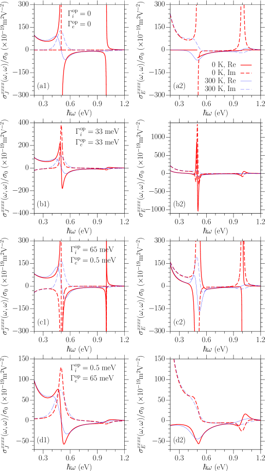
Figure 8: (color online) Spectra of $\sigma_{J}^{xxxx}(\omega,\omega)$ (left column) and $\sigma_{E}^{xxxx}(\omega,\omega)$ (right column) for different optical relaxation parameters at zero temperature (thick red curves) and at room temperatures (thin blue curves); $|\mu|=0.5$ eV. Solid (dashed) curves give their real ( imaginary) parts. In calculating $\sigma_{E}^{xxxx}(\omega,\omega)$, $\Gamma_{e}^{\text{dc}}=\Gamma_{e}^{\text{op}}$ and $\Gamma_{i}^{\text{dc}}=0$.

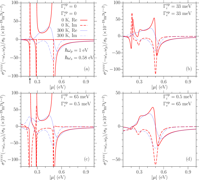
Figure 9: (color online) Chemical potential $|\mu|$ dependence of $\sigma_{J}^{dabc}(-\omega_{s},\omega_{p})$ for different optical relaxation parameters at zero temperature (thick red curves) and at room temperatures (thin blue curves); $\hbar\omega_{s}=0.58$ eV and $\hbar\omega_{p}=1$ eV. The real (imaginary) parts are given by solid (dashed) curves. The arrow in (a) indicates the vertical line there corresponding to the derivative of a $\delta$ function.

IV.1 DC current induced SHG

We first consider dc-induced second harmonic generation, governed by $\sigma^{(3);dabc}(\omega,\omega,0)$. For monochromatic light at frequency $\omega$, the second order optically induced current is given by

$$\bm{J}^{(3)}_{\text{SHG}}(\omega)=2\sigma_{\text{SHG}}^{A}(\omega)\bm{E}_{\omega}\bm{E}_{\omega}\cdot\bm{E}_{\text{dc}}+\sigma_{\text{SHG}}^{B}(\omega)\bm{E}_{\text{dc}}\bm{E}_{\omega}\cdot\bm{E}_{\omega}\,.$$ (73)

There the two nonzero components are $\sigma_{\text{SHG}}^{A}(\omega)=3\sigma^{(3);xxyy}(\omega,\omega,0)$ and $\sigma_{\text{SHG}}^{B}(\omega)=3\sigma^{(3);xyyx}(\omega,\omega,0)$. Correspondingly, each of them includes two parts: the dc-current induced second harmonic generation (CSHG) $\sigma^{(3)}_{J}$ and the dc-field induced second harmonic generation (EFISH) $\sigma^{(3)}_{E}$.

In Fig. 8 we plot the photon energy dependence of $\sigma_{J/E}^{dabc}(\omega,\omega)$ for $|\mu|=0.5$ eV and different values of optical relaxation parameters $\Gamma_{e}^{\text{op}}$ and $\Gamma_{i}^{\text{op}}$ at zero and room temperature. Two resonant peaks appear for both $\sigma_{J}^{dabc}$ and $\sigma_{E}^{dabc}$, one at $\hbar\omega=|\mu|$ and one at $2|\mu|$. The first corresponds to the second harmonic resonant with the onset of one-photon absorption, and the second to the fundamental resonant with the onset of one-photon absorption; the first peak leads to a higher response coefficients than the second. In general, $\sigma_{J}^{xxxx}$ and $\sigma_{E}^{xxxx}$ are of the same order of magnitude. Therefore, in a high mobility graphene sample with a small $\Gamma_{i}^{\text{dc}}$, the contribution of $\sigma_{J}^{dabc}(\omega,\omega)$ dominates $\sigma^{(3);dabc}(\omega,\omega,0)$ because of the prefactor ${\text{1eV}}/{\Gamma_{i}^{\text{dc}}}$ (see Eq. (69)).

From Eq. (70), we see that the first resonance in $\sigma_{J}^{dabc}(\omega)$ is determined by ${\cal H}_{\mu}(2\hbar\omega+i\Gamma_{e}^{\text{op}})$ and ${\cal I}_{\mu}(2\hbar\omega+i\Gamma_{e}^{\text{op}})$; the other resonance is determined only by ${\cal H}_{\mu}(\hbar\omega+i\Gamma_{e}^{\text{op}})$. Obviously, for both transitions smaller values of $\Gamma_{e}^{\text{op}}$ result in a larger value and a sharper peak. At room temperature, these peaks are broadened and lowered. The vertical line at $\hbar\omega=|\mu|$ in Fig. 8 (a1) comes from $\text{Im}[{\cal H}_{\mu}(2\hbar\omega+i\Gamma_{e}^{\text{op}})]$ as $\Gamma_{e}^{\text{op}}\to 0$, which is proportional to $\delta(\hbar\omega-|\mu|)$; the peak in Fig. 8 (c1) shows the fine structure of $\text{Im}[{\cal I}_{\mu}(2\hbar\omega+i\Gamma_{e}^{\text{op}})]$ for $\Gamma_{e}^{\text{op}}=0.5$ meV (see Appendix B). However, it is interesting to note that these two fine structures undergo important changes at room temperature: In Fig. 8 (a1), we see that the first fine structure leads to a peak with broadened width; in Fig. 8 (c1), we see that the second fine structure leads to a sign change around $\hbar\omega=|\mu|$ when the temperature increases from zero to room temperature.

IV.2 DC current induced difference frequency

A counterpart of the third order parametric frequency conversion discussed in Section III.4 is difference frequency generation which is, like second harmonic generation, a second order nonlinear effect that can be induced in graphene when applying a dc field. With a strong pump at frequency $\omega_{p}$, difference frequency generation converts a signal frequency $\omega_{s}$ to a new frequency $\omega_{p}-\omega_{s}$; the response is determined by $\sigma^{(3);dabc}(-\omega_{s},\omega_{p},0)$. Similar to dc-induced second harmonic generation, there are current and electric field contributions to dc-induced difference frequency generation. As we found in Section IV.1 for dc-induced second harmonic generation, the current contribution should dominate the dc-induced difference frequency generation in a high mobility sample. As an example, we plot the chemical potential dependence of $\sigma^{(3);dabc}_{J}(-\omega_{s},\omega_{p})$ for different optical relaxation parameters in Fig. 9 for $\hbar\omega_{p}=1$ eV (with a wavelength of about $1.24~{}\mu$m) and $\hbar\omega_{s}=0.58$ eV (with a wavelength of about $2.1~{}\mu$m). For vanishing optical relaxation parameters ($\Gamma_{i}^{\text{op}}=\Gamma_{e}^{\text{op}}=0$), it is clear from Fig. 9 (a) that there are three resonant transitions in the plotted chemical potential range: $|\mu_{1}|=(\hbar\omega_{p}-\hbar\omega_{s})/2=0.21$ eV, $|\mu_{2}|=\hbar\omega_{s}/2=0.29$ eV, and $|\mu_{3}|=\hbar\omega_{p}/2=0.5$ eV. Without relaxation, the imaginary part of the conductivity is always zero except at these three resonant transitions (shown as vertical lines): the first is given by $\lim\limits_{\delta\to 0}\text{Im}[{\cal I}_{\mu}(\hbar\omega_{p}-\hbar\omega_{s}+i\delta)]\propto\frac{d}{d|\mu|}\delta(\hbar\omega_{p}-\hbar\omega_{s}-|\mu|)$, the other two are given by $\lim\limits_{\delta\to 0}\text{Im}[{\cal H}_{\mu}(-\hbar\omega_{s}+i\delta)]\propto\delta(\hbar\omega_{s}-|\mu|)$ and $\lim\limits_{\delta\to 0}\text{Im}[{\cal H}_{\mu}(\hbar\omega_{p}+i\delta)]\propto\delta(\hbar\omega_{p}-|\mu|)$. With finite relaxation rates or at finite temperature, the vertical lines are broadened to structures of finite strength and width.

IV.3 Comparison between calculations and experiments

Bykov et al. Bykov et al. (2012) observed that SHG radiation from a graphene/SiO₂/Si(001) substrate strongly depends on the applied current density in the graphene layer, which is attributed to the CSHG effect of graphene. A similar structure was also studied by An et al. An et al. (2013, 2014), who could measure the radiation from different locations on the graphene sheet; they interpreted the result as EFISH, where the electric field is induced by current-associated trapped charge at the graphene/SiO₂ interface. Because of the interface contribution to the SHG radiation Dean and van Driel (2009, 2010); Bykov et al. (2012); An et al. (2013, 2014), the contribution of the current related SHG from the graphene is hard to extract.

The best way of measuring the dc-induced second order nonlinearity of graphene, without any background contribution from interface effects, would be to mount graphene in a symmetric structure; this can be difficult. However, within the framework of the experiments of the type that have already been done, we can suggest a strategy that might help identify the in-plane graphene CSHG(EFISH) by the azimuthal angle dependence of the generated signal. For linearly polarized light with $\bm{E}_{\omega}=E_{\omega}\begin{pmatrix}\cos\phi\\ \sin\phi\end{pmatrix}$ and $\bm{E}_{\text{dc}}=E_{\text{dc}}\begin{pmatrix}\cos\phi_{J}\\ \sin\phi_{J}\end{pmatrix}$, Eq. (73) becomes

$$\bm{J}^{(3)}_{\text{SHG}}(\omega) = E_{\omega}^{2}E_{\text{dc}}\Big{\{}\sigma_{1}(\omega)\begin{pmatrix}\cos(2\phi-\phi_{J})\\ \sin(2\phi-\phi_{J})\end{pmatrix}$$ (74)

$$+[\sigma_{1}(\omega)+\sigma_{2}(\omega)]\begin{pmatrix}\cos\phi_{J}\\ \sin\phi_{J}\end{pmatrix}\Big{\}}\,.$$

We see that the Cartesian components of the induced current vary as cosinusoidal functions of $0\phi$ (that is, independent of $\phi)$ and $2\phi$. In a short-hand notation, we will characterize these as $0\phi$ and $2\phi$ dependences. In most experiments Dean and van Driel (2009, 2010); Bykov et al. (2012); An et al. (2013, 2014), the graphene sample is mounted on a SiO₂/Si substrate, where the interface between SiO₂ and Si gives an interface-induced SHG and the bulk Si gives an electric quadrupole/magnetic dipole induced SHG. But for different crystal orientations of the Si substrate, the dependence of the combined interface and bulk contributions on azimuthal angle will be different Sipe et al. (1987): For the (111) face, the second harmonic radiation depends on the angle as $0\phi$ and $3\phi$; for the (001) face, the dependence is $0\phi$ and $4\phi$; while for the (110) face, the dependence becomes $0\phi$, $2\phi$, and $4\phi$. Therefore, from the azimuthal dependence of the SHG signal it might be possible to distinguish the graphene CSHG (EFISH) from the interface contributions, for example by putting graphene on top of different SiO₂/Si structures, one with the (111) face of Si normal to the interface and one with the (001) face normal. Because of the same origin of CSHG and EFISH in graphene, they would have the same angle dependence, so such experiments would not help to distinguish between these different contributions from graphene; but for a heavily doped and high mobility graphene sample our calculations show that the CSHG should dominate.

V Conclusion and Discussion

Perturbative analyses play a central role in nonlinear optics. Even when the electrons in a material are treated as independent, and relaxation is only described phenomenologically, the calculated response tensors that relate the induced polarization or current to powers of the applied fields indicate the nonlinear optical effects that are allowed, and point to where resonances can lead to an interesting dependence on time and frequency. Often more sophisticated models of the electron dynamics are required, and sometimes the perturbative framework itself is insufficient to address the physics of interest. But even then these kinds of perturbative treatments provide a starting point for more realistic calculations.

In this paper we have provided such a treatment of the nonlinear third order optical response of doped graphene, with the main goal of investigating the effects of phenomenological relaxation parameters, finite temperature, and laser pulse width on the induced currents. We focused on the contributions of optical transitions around the Dirac points, where the widely used linear dispersion relation is a good approximation. By solving semiconductor Bloch equations perturbatively, an analytic expression for general third order conductivities was obtained at zero temperature, taking different relaxation parameters for interband and intraband optical transitions. The nonlinear conductivities at finite temperature were obtained by an appropriate integration over the chemical potential. The conductivities show a complicated dependence on photon energy, chemical potential, and the relaxation parameters.

Even with the inclusion of relaxation we found that the perturbative approach itself is problematic at vanishing chemical potential, as might be expected from a similar result in the semiclassical limit Mikhailov (2007), except in the special case that either first- or third-order interband and intraband relaxation rates are set equal. The perturbative approach adopted is unproblematic for doped graphene at zero temperature, but is a concern at finite temperature, since thermal fluctuations always place some electrons or holes near the Dirac points. Yet numerical calculations of the full semiconductor Bloch equations indicate that the contribution of such electrons to the full optical response is small, so this effect does not afflict our results.

We discussed in detail different nonlinear effects, including third harmonic generation, Kerr effects and two-photon absorption, two-color coherent current injection, parametric frequency conversion, and dc-current and -field induced second harmonic generation and difference frequency generation. The interband relaxation generally broadens and lowers the resonant peaks, while the intraband relaxation plays an important role in some of the effects, including two-color coherent current injection and the dc-current induced second order nonlinearities. At room temperature most of the resonant structures are smeared out.

We also considered the response of graphene to laser pulses. The optical response depends in detail on the frequency width of the incident pulse and the frequency structure of the response tensors. The two natural limits are (1) when the frequency structure of the response coefficients is rather flat on the scale of the frequency width of the incident pulse, and the induced current follows the injecting pulses, and (2) when there are divergences in the response coefficients at frequencies close to the real axis, as for two-color coherent control, the a dynamics associated directly with the relaxation processes.

Comparison of our results with experiments is difficult, since in many of the reported experiments the graphene samples have not been characterized in the linear regime, and neither the relaxation parameters nor even the chemical potential have been identified. Results for some nonlinear response coefficients, such as that describing the Kerr effect, are predicted by our calculations to be so sensitive to these parameters that we cannot hazard a comparison of theory to experiment. Yet our results for third harmonic generation and parametric frequency conversion are insensitive enough to these parameters that we can conclude our results are about two orders of magnitude smaller than those extracted from experiments Cheng et al. (2014a), even with the adoption of reasonable relaxation parameters. We speculated on the causes of this disagreement; it is of course early days for both detailed experimental and theoretical studies of such nonlinear effects in graphene. But these disagreements may persist, and a long and difficult journey may be necessary to understand the details of the full nonlinear optical response of graphene. Even so we can expect that, as in the study of the nonlinear optical response of other materials, the kind of perturbative calculation we have presented here will provide a useful port of embarkation, paving the way to a better physical insight in the complex nonlinear optical response of graphene.

Appendix A Perturbation solution of Semiconductor Bloch equation

We describe the electronic states in graphene by the tight binding model employing carbon $2p_{z}$ orbitals with only nearest neighbor coupling. Neglecting the overlap between different $p_{z}$ orbitals, the band structure that results is electron-hole symmetric with energies $\varepsilon_{+\bm{k}}=-\varepsilon_{-\bm{k}}$ where $+(-)$ is the band index for $\pi^{\ast}(\pi)$ bands, and the Berry connections satisfy $\bm{\xi}_{s\bar{s}\bm{k}}=\bm{\xi}_{\bar{s}s\bm{k}}\equiv\bm{r}_{\bm{k}}$ and $\bm{\xi}_{ss\bm{k}}=\bm{\xi}_{\bar{s}\bar{s}\bm{k}}$ where $s=\pm$ is the band index and $\bar{s}$ is the index of the band that is not the $s$ band Cheng et al. (2014a). Up to the dipole approximation of light-matter interaction, the SBE in Eq. (7) can be expanded as

$$\hbar\frac{\partial\rho_{ss\bm{k}}^{(n)}(t)}{\partial t} = ie\bm{E}(t)\cdot\bm{r}_{\bm{k}}(\rho_{\bar{s}s\bm{k}}^{(n-1)}-\rho_{s\bar{s}\bm{k}}^{(n-1)})$$

$$- e\bm{E}(t)\cdot\bm{\nabla}_{\bm{k}}\rho_{ss\bm{k}}^{(n-1)}-\Gamma_{i}^{(n)}\rho_{ss\bm{k}}^{(n)}\,,$$

$$\hbar\frac{\partial\rho_{s\bar{s}\bm{k}}^{(n)}(t)}{\partial t} = -is\epsilon_{\bm{k}}\rho_{s\bar{s}\bm{k}}^{(n)}(t)+ie\bm{E}(t)\cdot\bm{r}_{\bm{k}}(\rho_{\bar{s}\bar{s}\bm{k}}^{(n-1)}-\rho_{ss\bm{k}}^{(n-1)})$$ (75)

$$- e\bm{E}(t)\cdot\bm{\nabla}_{\bm{k}}\rho_{s\bar{s}\bm{k}}^{(n-1)}-\Gamma_{e}^{(n)}\rho_{s\bar{s}\bm{k}}^{(n)}\,,$$

with $\epsilon_{\bm{k}}=\varepsilon_{+\bm{k}}-\varepsilon_{-\bm{k}}$. In Eq. (75) the terms involving $\bm{r}_{\bm{k}}$ give the interband contribution, and the terms involving $\bm{\nabla}_{\bm{k}}$ give the intraband contribution. Treating the electric field term perturbatively, the first three terms are expanded as

$$\rho_{s_{1}s_{2}\bm{k}}^{(1)}(t) = \int\frac{d\omega_{3}}{2\pi}(-e)E_{\omega_{3}}^{c}e^{-i\omega_{3}t}{\cal P}^{(1);c}_{s_{1}s_{2}\bm{k}}(\omega_{3})$$

$$\rho_{s_{1}s_{2}\bm{k}}^{(2)}(t) = \int\frac{d\omega_{2}d\omega_{3}}{(2\pi)^{2}}(-e)^{2}E_{\omega_{2}}^{b}E_{\omega_{3}}^{c}e^{-i\omega_{0}t}{\cal P}^{(2);bc}_{s_{1}s_{2}\bm{k}}(\omega_{2},\omega_{3})$$

$$\rho_{s_{1}s_{2}\bm{k}}^{(3)}(t) = \int\frac{d\omega_{1}d\omega_{2}d\omega_{3}}{(2\pi)^{3}}(-e)^{3}E_{\omega_{1}}^{a}E_{\omega_{2}}^{b}E_{\omega_{3}}^{c}e^{-i\omega t}$$ (76)

$$\times{\cal P}^{(3);abc}_{s_{1}s_{2}\bm{k}}(\omega_{1},\omega_{2},\omega_{3})\,,$$

with $\omega_{0}=\omega_{2}+\omega_{3}$ and $\omega=\omega_{1}+\omega_{0}$. By substituting the above expansion into Eq. (75), we get the following equations for ${\cal P}^{(i)}$.

(1) The linear order terms are determined by

$$\nu_{3}{\cal P}^{(1);c}_{ss\bm{k}}(\omega_{3}) = i\frac{\partial n_{s\bm{k}}}{\partial k_{c}}\,,$$

$$(\vartheta_{3}-s\epsilon_{\bm{k}}){\cal P}^{(1);c}_{s\bar{s}\bm{k}}(\omega_{3}) = -sr^{c}_{\bm{k}}\Delta n_{\bm{k}}\,.$$ (77)

Here we have put $\Delta n_{\bm{k}}=n_{+\bm{k}}-n_{-\bm{k}}$. The solutions are

$${\cal P}^{(1);c}_{ss\bm{k}}(\omega_{3})=\frac{i}{\nu_{3}}\frac{\partial n_{s\bm{k}}}{\partial k_{c}}\,,\quad{\cal P}^{(1);c}_{s\bar{s}\bm{k}}(\omega_{3})=\frac{-sr_{\bm{k}}^{c}\Delta n_{\bm{k}}}{\vartheta_{3}-s\epsilon_{\bm{k}}}\,,$$ (78)

which leads to the linear conductivity:

$$\sigma^{(1);da}(\omega)=-e^{2}\sum_{s_{1}s_{2}}\int\frac{d\bm{k}}{4\pi^{2}}v_{s_{2}s_{1}\bm{k}}^{d}{\cal P}^{(1);a}_{s_{1}s_{2}\bm{k}}(\omega)\,.$$ (79)

Here $\bm{v}_{s_{1}s_{2}\bm{k}}$ are the matrix elements of the velocity operator, which satisfy $\bm{v}_{++\bm{k}}=-\bm{v}_{--\bm{k}}$ and $\bm{v}_{+-\bm{k}}=-\bm{v}_{-+\bm{k}}$ in the tight binding model we have adopted.

(2) The second order terms are determined by

$$\nu_{0}{\cal P}^{(2);bc}_{ss\bm{k}}(\omega_{2},\omega_{3}) = r_{\bm{k}}^{b}[{\cal P}^{(1);c}_{\bar{s}s\bm{k}}(\omega_{3})-{\cal P}^{(1);c}_{s\bar{s}\bm{k}}(\omega_{3})]$$

$$+i\frac{\partial}{\partial k_{b}}{\cal P}^{(1);c}_{ss\bm{k}}(\omega_{3})\,,$$

$$(\vartheta_{3}-s\epsilon_{\bm{k}}){\cal P}^{(2);bc}_{s\bar{s}\bm{k}}(\omega_{2},\omega_{3}) = r^{b}_{\bm{k}}\left[{\cal P}^{(1);c}_{\bar{s}\bar{s}\bm{k}}(\omega_{3})-{\cal P}^{(1);c}_{ss\bm{k}}(\omega_{3})\right]$$ (80)

$$+i\frac{\partial}{\partial k_{b}}{\cal P}^{(1);c}_{s\bar{s}\bm{k}}(\omega_{3})\,,$$

The solutions are

$${\cal P}^{(2);bc}_{ss\bm{k}}(\omega_{2},\omega_{3}) = \frac{i}{\nu_{0}}\left[\frac{i}{\nu_{3}}\frac{\partial^{2}n_{s\bm{k}}}{\partial k_{b}\partial k_{c}}\right.$$

$$\left.+sr_{\bm{k}}^{b}r_{\bm{k}}^{c}\Delta n_{\bm{k}}\left(\frac{1}{\vartheta_{3}+\epsilon_{\bm{k}}}+\frac{1}{\vartheta_{3}-\epsilon_{\bm{k}}}\right)\right]\,,$$

$${\cal P}^{(2);bc}_{s\bar{s}\bm{k}}(\omega_{2},\omega_{3}) = \frac{-is}{\vartheta_{0}-s\epsilon_{\bm{k}}}\left[\frac{\partial}{\partial k_{b}}\left(\frac{r_{\bm{k}}^{c}\Delta n_{\bm{k}}}{\vartheta_{3}-s\epsilon_{\bm{k}}}\right)+\frac{r_{\bm{k}}^{b}}{\nu_{3}}\frac{\partial\Delta n_{\bm{k}}}{\partial k_{c}}\right]\,,$$

Because the graphene crystal structure is centrosymmetric, its second order conductivity is zero.

(3) The third order terms are determined by

$$\nu{\cal P}^{(3);abc}_{ss\bm{k}} = r_{\bm{k}}^{b}[{\cal P}^{(2);bc}_{\bar{s}s\bm{k}}(\omega_{2},\omega_{3})-{\cal P}^{(2);bc}_{s\bar{s}\bm{k}}(\omega_{2},\omega_{3})]$$

$$+ i\frac{\partial}{\partial k_{b}}{\cal P}^{(2);bc}_{ss\bm{k}}(\omega_{2},\omega_{3})\,,$$

$$(\vartheta-s\epsilon_{\bm{k}}){\cal P}^{(3);abc}_{s\bar{s}\bm{k}} = r^{b}_{\bm{k}}\left[{\cal P}^{(2);bc}_{\bar{s}\bar{s}\bm{k}}(\omega_{2},\omega_{3})-{\cal P}^{(2);bc}_{ss\bm{k}}(\omega_{2},\omega_{3})\right]$$ (81)

$$+ i\frac{\partial}{\partial k_{b}}{\cal P}^{(2);bc}_{s\bar{s}\bm{k}}(\omega_{2},\omega_{3})\,,$$

The frequency dependence of ${\cal P}^{(3);dabc}_{s_{1}s_{2}\bm{k}}(\omega_{1},\omega_{2},\omega_{3})$ is implicit. The solutions can be written as

$${\cal P}^{(3);abc}_{ss\bm{k}} = \frac{1}{\nu\nu_{0}\nu_{3}}P^{abc}_{1;s\bm{k}}+\frac{1}{\nu\nu_{0}}P^{abc}_{2;s\bm{k}}(\vartheta_{3})$$

$$+ \frac{1}{\nu\nu_{3}}P^{abc}_{3;s\bm{k}}(\vartheta_{0})+\frac{1}{\nu}P^{abc}_{4;s\bm{k}}(\vartheta_{0},\vartheta_{3})\,,$$

$${\cal P}^{(3);abc}_{s\bar{s}\bm{k}} = \frac{1}{\nu_{0}\nu_{3}}P^{abc}_{5;s\bm{k}}(\vartheta)+\frac{1}{\nu_{0}}P^{abc}_{6;s\bm{k}}(\vartheta,\vartheta_{3})$$ (82)

$$+ \frac{1}{\nu_{3}}P^{abc}_{7;s\bm{k}}(\vartheta,\vartheta_{0})+P^{abc}_{8;s\bm{k}}(\vartheta,\vartheta_{0},\vartheta_{3})\,,$$

Here terms $P^{abc}_{i;s\bm{k}}$ with $i=1,\cdots,4$ are related to the populations at band $s$ and are given by

$$P^{abc}_{1;s\bm{k}} = -i\frac{\partial^{3}n_{s\bm{k}}}{\partial k_{a}\partial k_{b}\partial k_{c}}\,,$$

$$P^{abc}_{2;s\bm{k}}(\vartheta_{3}) = -s\frac{\partial}{\partial k_{a}}\left[r_{\bm{k}}^{b}r_{\bm{k}}^{c}\Delta n_{\bm{k}}\left(\frac{1}{\vartheta_{3}+\epsilon_{\bm{k}}}+\frac{1}{\vartheta_{3}-\epsilon_{\bm{k}}}\right)\right]\,,$$

$$P^{abc}_{3;s\bm{k}}(\vartheta_{0}) = -sr_{\bm{k}}^{a}r_{\bm{k}}^{b}\left(\frac{1}{\vartheta_{0}+\epsilon_{\bm{k}}}+\frac{1}{\vartheta_{0}-\epsilon_{\bm{k}}}\right)\frac{\partial\Delta n_{\bm{k}}}{\partial k_{c}}\,,$$

$$P^{abc}_{4;s\bm{k}}(\vartheta_{0},\vartheta_{3}) = -sr_{\bm{k}}^{a}\left[\frac{1}{\vartheta_{0}+\epsilon_{\bm{k}}}\frac{\partial}{\partial k_{b}}\left(\frac{r_{\bm{k}}^{c}\Delta n_{\bm{k}}}{\vartheta_{3}+\epsilon_{\bm{k}}}\right)\right.$$

$$\left.+\frac{1}{\vartheta_{0}-\epsilon_{\bm{k}}}\frac{\partial}{\partial k_{b}}\left(\frac{r_{\bm{k}}^{c}\Delta n_{\bm{k}}}{\vartheta_{3}-\epsilon_{\bm{k}}}\right)\right]\,,$$

while the terms $P^{abc}_{i;s\bm{k}}$ with $i=5,\cdots,8$ are related to the interband polarization and are given by

$$P^{abc}_{5;s\bm{k}}(\vartheta) = s\frac{r_{\bm{k}}^{a}}{\vartheta-s\epsilon_{\bm{k}}}\frac{\partial^{2}\Delta n_{\bm{k}}}{\partial k_{b}\partial k_{c}}\,,$$

$$P^{abc}_{6;s\bm{k}}(\vartheta,\vartheta_{3}) = -2is\frac{r_{\bm{k}}^{a}r_{\bm{k}}^{b}r_{\bm{k}}^{c}\Delta n_{\bm{k}}}{\vartheta-s\epsilon_{\bm{k}}}\left(\frac{1}{\vartheta_{3}+\epsilon_{\bm{k}}}+\frac{1}{\vartheta_{3}-\epsilon_{\bm{k}}}\right)\,,$$

$$P^{abc}_{7;s\bm{k}}(\vartheta,\vartheta_{0}) = \frac{i}{\vartheta-s\epsilon_{\bm{k}}}\frac{\partial}{\partial k_{a}}\left(r_{\bm{k}}^{b}\frac{\partial\Delta n_{\bm{k}}}{\partial k_{c}}\right)\,,$$

$$P^{abc}_{8;s\bm{k}}(\vartheta,\vartheta_{0},\vartheta_{3}) = \frac{1}{\vartheta-s\epsilon_{\bm{k}}}\frac{\partial}{\partial k_{a}}\left\{\frac{1}{\vartheta_{0}-s\epsilon_{\bm{k}}}\right.$$

$$\left.\times\left[\frac{\partial}{\partial k_{b}}\left(\frac{r_{\bm{k}}^{c}\Delta n_{\bm{k}}}{\vartheta_{3}-s\epsilon_{\bm{k}}}\right)\right]\right\}\,.$$

The unsymmetrized third order conductivity which follows from these terms is

$$\widetilde{\sigma}^{(3);dabc}(\omega_{1},\omega_{2},\omega_{3}) = -e^{4}\sum_{s_{1}s_{2}}\int\frac{d\bm{k}}{4\pi^{2}}v_{s_{2}s_{1}\bm{k}}^{d}$$ (83)

$$\times{\cal P}^{(3);abc}_{s_{1}s_{2}\bm{k}}(\omega_{1},\omega_{2},\omega_{3})\,.$$

Then we find terms ${\cal S}_{i}$ in Eq. (15) are given by

$${\cal S}_{i}^{dabc}=-(i\sigma_{3})^{-1}e^{4}\int\!\!\frac{d\bm{k}}{4\pi^{2}}v_{++\bm{k}}^{d}\left(P^{abc}_{i;+\bm{k}}-P^{abc}_{i;-\bm{k}}\right)\,,$$

for $i=1,2,3,4$ and

$${\cal S}_{i}^{dabc}=(i\sigma_{3})^{-1}e^{4}\int\!\!\frac{d\bm{k}}{4\pi^{2}}v_{+-\bm{k}}^{d}\left(P^{abc}_{i;+\bm{k}}-P^{abc}_{i;-\bm{k}}\right)\,,$$

for $i=5,6,7,8$.

In this work, we only consider optical transitions around the Dirac points $\bm{K}=(\bm{b}_{1}+2\bm{b}_{2})/3$ or $\bm{K}^{\prime}=(\bm{b}_{2}+2\bm{b}_{1})/3$ with $\bm{b}_{1}$ and $\bm{b}_{2}$ the primitive reciprocal lattice vectors. These two Dirac cones are connected by the inversion symmetry, and they lead to the same contribution to the conductivities we consider, whether linear or third order. In the following, we calculate the conductivity around $\bm{K}$ explicitly and get the total results by considering both valley degeneracy $g_{v}=2$ and spin degeneracy $g_{s}=2$. Around the Dirac point $\bm{K}$, we approximate each quantity up to its lowest order of $\bm{k}-\bm{K}$: The electronic dispersion is $\varepsilon_{s\bm{K}+\bm{k}}=s\hbar v_{F}k$, the velocity matrix elements are $\bm{v}_{ss(\bm{K}+\bm{k})}\approx sv_{F}{\bm{k}}/{k}$ and $\bm{v}_{s\bar{s}(\bm{K}+\bm{k})}\approx isv_{F}\bm{k}\times{\hat{\bm{z}}}/{k}$, and the interband Berry connection is $\bm{r}_{\bm{K}+\bm{k}}\approx\bm{k}\times{\hat{\bm{z}}}/{2k^{2}}$. The linear conductivity that results is given by Eq. (11).

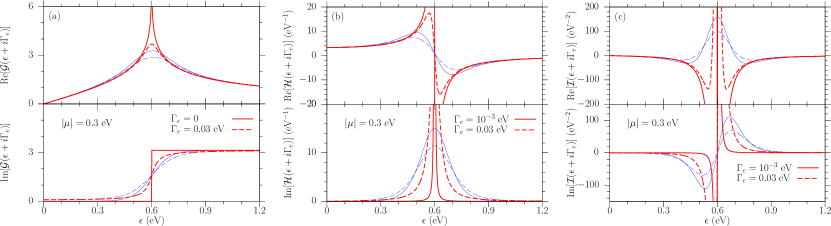
Figure 10: (color online) $\epsilon$ dependence of (a) ${\cal G}_{\mu}(\epsilon+i\Gamma)$ and $\overline{\cal G}_{\mu;T}(\epsilon+i\Gamma)$, (b) ${\cal H}_{\mu}(\epsilon+i\Gamma)$ and $\overline{\cal H}_{\mu;T}(\epsilon+i\Gamma)$, (c) ${\cal I}_{\mu}(\epsilon+i\Gamma)$ and $\overline{\cal I}_{\mu;T}(\epsilon+i\Gamma)$. Solid (dashed) curves are for $\Gamma=0$ ($\Gamma=0.03$ eV), and thick red (thin blue) curves are for the function without (with) a temperature average. Other parameters are $|\mu|=0.3$ eV and $T=300$ K.

In calculating the integrals over $\bm{k}$ necessary to evaluate the third order conductivities, we use the relation

$$\dfrac{\partial\epsilon_{\bm{k}}}{\partial k_{a}} = 2v_{++\bm{k}}^{a}\,,$$ (84)

$$\dfrac{\partial r_{\bm{k}}^{a}}{\partial k_{b}} = \dfrac{2i}{\epsilon_{\bm{k}}^{2}}(v_{++\bm{k}}^{a}v_{+-\bm{k}}^{b}+v_{+-\bm{k}}^{b}v_{++\bm{k}}^{a})\,,$$ (85)

$$\dfrac{\partial v_{++\bm{k}}^{a}}{\partial k_{b}} = -2\dfrac{v_{+-\bm{k}}^{a}v_{+-\bm{k}}^{b}}{\epsilon_{\bm{k}}}\,,$$ (86)

$$\dfrac{\partial v_{+-\bm{k}}^{a}}{\partial k_{b}} = -2\dfrac{v_{++\bm{k}}^{a}v_{+-\bm{k}}^{b}}{\epsilon_{\bm{k}}}\,,$$ (87)

to expand the derivatives in ${\cal S}_{i}$, and find that all the required integrations over $\bm{k}$ can be related to

$$g_{s}g_{v}\frac{e^{4}}{\Omega} \int\!\!\frac{d\bm{k}}{(2\pi)^{2}}v_{+-\bm{k}}^{d}v_{+-\bm{k}}^{a}v_{++\bm{k}}^{b}v_{++\bm{k}}^{c}\delta(\epsilon_{\bm{k}}-\Omega)=\frac{1}{4}\sigma_{3}A_{1}\,,$$

$$g_{s}g_{v}\frac{e^{4}}{\Omega} \int\!\!\frac{d\bm{k}}{(2\pi)^{2}}v_{+-\bm{k}}^{d}v_{+-\bm{k}}^{a}v_{+-\bm{k}}^{b}v_{+-\bm{k}}^{c}\delta(\epsilon_{\bm{k}}-\Omega)=\frac{1}{4}\sigma_{3}A_{0}\,,$$

Using partial fractions and taking the integral over $\Omega$, we obtain all the ${\cal S}_{i}$ given in Eq. (19-26)

Appendix B Temperature Effects

In this appendix we discuss how the temperature affects the contributions to the conductivities from ${\cal G}_{\mu}(\epsilon+i\Gamma_{e})$, ${\cal H}_{\mu}(\epsilon+i\Gamma_{e})$, and ${\cal I}_{\mu}(\epsilon+i\Gamma_{e})$.

(1) ${\cal G}_{\mu}(\epsilon+i\Gamma_{e})$: At finite temperature, this is replaced by $\overline{\cal G}_{\mu;T}(\epsilon+i\Gamma_{e})$ with

$$\overline{\cal G}_{\mu;T}(\epsilon+i\Gamma_{e})=\beta\int_{-\infty}^{\infty}dxF_{\mu}(x,T)[1-F_{\mu}(x,T)]{\cal G}_{x}(\epsilon+i\Gamma_{e})\,.$$ (88)

As $\Gamma_{e}\to 0$, ${\cal G}_{\mu}(\epsilon+i\Gamma_{e})$ diverges logarithmically at $\epsilon=\pm 2|\mu|$, while $\overline{\cal G}_{\mu;T}(\epsilon+i\Gamma_{e})$ is smooth. Both functions are smooth as $\epsilon+i\Gamma_{e}\to 0$. In Fig. 10 (a) both ${\cal G}_{\mu}(\epsilon+i\Gamma_{e})$ and $\overline{\cal G}_{\mu;T}(\epsilon+i\Gamma_{e})$ are plotted for $\Gamma_{e}=0$ and $\Gamma_{e}=0.03$ eV at $|\mu|=0.3$ eV and $T=300$ K. Moving from zero to finite temperature, a finite $T$ has an effect similar to the inclusion of relaxation: Both remove the singularity and broaden the peak and step function.

(2) ${\cal H}_{\mu}(\epsilon+i\Gamma_{e})$: At finite temperature, this is replaced by $\overline{\cal H}_{\mu;T}(\epsilon+i\Gamma_{e})$ with

$$\overline{\cal H}_{\mu;T}(\epsilon+i\Gamma_{e})=\beta\int_{-\infty}^{\infty}dxF_{\mu}(x,T)[1-F_{\mu}(x,T)]{\cal H}_{x}(\epsilon+i\Gamma_{e})\,.$$ (89)

At $|\mu|\to z_{0}$ with $2z_{0}=\epsilon+i\Gamma_{e}$ for $\epsilon>0$, ${\cal H}_{\mu}(\epsilon+i\Gamma_{e})$ diverges as $(|\mu|-z_{0})^{-1}$. In the relaxation free limit for nonzero $\epsilon$ we can write

$$\frac{1}{|\mu|-\epsilon-i\Gamma_{e}}\stackrel{{\scriptstyle\Gamma_{e}\to 0}}{{\longrightarrow}}P.\frac{1}{|\mu|-\epsilon}+i\pi\delta(|\mu|-\epsilon)\,,$$ (90)

where $P.$ means the integration takes the principal part; thus the imaginary part of ${\cal H}_{\mu}$ tends to a $\delta$ function. However, both the real and imaginary parts of $\overline{\cal H}_{\mu;T}$ are smooth for $\epsilon>0$ or $\epsilon=0$ and $\Gamma_{e}\neq 0$. For small $\Gamma_{e}$, $\overline{\cal H}_{\mu;T}(i\Gamma_{e})\propto\ln\Gamma_{e}$.

In Fig. 10 (b) both ${\cal H}_{\mu}(\epsilon+i\Gamma_{e})$ and $\overline{\cal H}_{\mu;T}(\epsilon+i\Gamma_{e})$ are plotted for $\Gamma_{e}=10^{-3}$ eV and $\Gamma_{e}=0.03$ eV at $\mu=0.3$ eV and $T=300$ K. The inclusion of finite temperature leads to a broadening of the $\delta$-function-like imaginary part.

(3) ${\cal I}_{\mu}(\epsilon+i\Gamma_{e})$: At finite temperature, this is replaced by $\overline{\cal I}_{\mu;T}(\epsilon+i\Gamma_{e})$ with

$$\overline{\cal I}_{\mu;T}(\epsilon+i\Gamma_{e})=\beta\int_{-\infty}^{\infty}dxF_{\mu}(x,T)[1-F_{\mu}(x,T)]{\cal I}_{x}(\epsilon+i\Gamma_{e})\,.$$ (91)

At $|\mu|\to z_{0}$ with $2z_{0}=\epsilon+i\Gamma_{e}$ for $\epsilon>0$, ${\cal I}_{\mu}(\epsilon+i\Gamma_{e})$ diverges as $(|\mu|-z_{0})^{-2}$. Around $\epsilon=2|\mu|$, $\text{Re}[{\cal I}_{\mu}(\epsilon+i\Gamma_{e})]$ has two minima $\sim-\Gamma_{e}^{-2}/2$ around $\epsilon\approx 2|\mu|\pm\sqrt{3}\Gamma_{e}$ and a maximum $\sim\Gamma_{e}^{-2}$ at $\epsilon=2|\mu|$, while $\text{Im}[{\cal I}_{\mu}(\epsilon+i\Gamma_{e})]$ has two extrema at $\epsilon\sim 2|\mu|\pm\Gamma_{e}/\sqrt{3}$ with values $\sim\pm 3\sqrt{3}/(8\Gamma_{e}^{2})$. These indicate that this function varies very fast around $\epsilon=2|\mu|$ for very small $\Gamma_{e}$. In a manner similar to the ${\cal H}$ function, at room temperature $\overline{\cal I}_{\mu;T}$ is a smooth function with respect to $\epsilon>0$ for any $\Gamma_{e}\geq 0$, and $\overline{\cal I}_{\mu;T}(i\Gamma_{e})\propto\Gamma_{e}^{-1}$.

In Fig. 10 (c) both ${\cal I}_{\mu}(\epsilon+i\Gamma_{e})$ and $\overline{\cal I}_{\mu;T}(\epsilon+i\Gamma_{e})$ are plotted for $\Gamma_{e}=10^{-3}$ eV and $\Gamma_{e}=0.03$ eV at $|\mu|=0.3$ eV and $T=300$ K.

References

- Castro Neto et al. (2009) A. H. Castro Neto, F. Guinea, N. M. R. Peres, K. S. Novoselov, and A. K. Geim, Rev. Mod. Phys. 81, 109 (2009).
- Bonaccorso et al. (2010) F. Bonaccorso, Z. Sun, T. Hasan, and A. C. Ferrari, Nat. Photon. 4, 611 (2010).
- Gu et al. (2012) T. Gu, N. Petrone, J. F. McMillan, A. van der Zande, M. Yu, G. Q. Lo, D. L. Kwong, J. Hone, and C. W. Wong, Nat. Photon. 6, 554 (2012).
- Glazov and Ganichev (2014) M. Glazov and S. Ganichev, Phys. Rep. 535, 101 (2014).
- Cheng et al. (2014a) J. L. Cheng, N. Vermeulen, and J. E. Sipe, New J. Phys. 16, 053014 (2014a).
- Cheng et al. (2014b) J. L. Cheng, N. Vermeulen, and J. E. Sipe, Opt. Express 22, 15868 (2014b).
- Novoselov et al. (2004) K. S. Novoselov, A. K. Geim, S. V. Morozov, D. Jiang, Y. Zhang, S. V. Dubonos, I. V. Grigorieva, and A. A. Firsov, Science 306, 666 (2004).
- Wang et al. (2008) F. Wang, Y. Zhang, C. Tian, C. Girit, A. Zettl, M. Crommie, and Y. R. Shen, Science 320, 206 (2008).
- Liu et al. (2011a) H. Liu, Y. Liu, and D. Zhu, J. Mater. Chem. 21, 3335 (2011a).
- Wülbern et al. (2010) J. H. Wülbern, S. Prorok, J. Hampe, A. Petrov, M. Eich, J. Luo, A. K.-Y. Jen, M. Jenett, and A. Jacob, Opt. Lett. 35, 2753 (2010).
- Matheisen et al. (2014) C. Matheisen, M. Waldow, B. Chmielak, S. Sawallich, T. Wahlbrink, J. Bolten, M. Nagel, and H. Kurz, Opt. Express 22, 5252 (2014).
- Ironside et al. (1993) C. Ironside, J. Aitchison, and J. Arnold, IEEE J. Quantum Electron. 29, 2650 (1993).
- Liu et al. (2014) W. Liu, L. Wang, and C. Fang, Appl. Phys. Lett. 104, 111114 (2014).
- Gandomkar and Ahmadi (2011) M. Gandomkar and V. Ahmadi, Opt. Lett. 36, 3825 (2011).
- Hagan et al. (1994) D. J. Hagan, Z. Wang, G. Stegeman, E. W. Van Stryland, M. Sheik-Bahae, and G. Assanto, Opt. Lett. 19, 1305 (1994).
- Ren et al. (2013) M.-L. Ren, X.-L. Zhong, B.-Q. Chen, and Z.-Y. Li, Chinese Phys. Lett. 30, 097301 (2013).
- Dean and van Driel (2009) J. J. Dean and H. M. van Driel, Appl. Phys. Lett. 95, 261910 (2009).
- Dean and van Driel (2010) J. J. Dean and H. M. van Driel, Phys. Rev. B 82, 125411 (2010).
- Bykov et al. (2012) A. Y. Bykov, T. V. Murzina, M. G. Rybin, and E. D. Obraztsova, Phys. Rev. B 85, 121413 (2012).
- An et al. (2013) Y. Q. An, F. Nelson, J. U. Lee, and A. C. Diebold, Nano Lett. 13, 2104 (2013).
- An et al. (2014) Y. Q. An, J. E. Rowe, D. B. Dougherty, J. U. Lee, and A. C. Diebold, Phys. Rev. B 89, 115310 (2014).
- Sipe et al. (1987) J. Sipe, D. Moss, and H. van Driel, Phys. Rev. B 35, 1129–1141 (1987).
- Mikhailov (2007) S. A. Mikhailov, Europhys. Lett. 79, 27002 (2007).
- Mikhailov and Ziegler (2008) S. A. Mikhailov and K. Ziegler, J. Phys. Condens. Matter 20, 384204 (2008).
- Glazov (2011) M. Glazov, JETP Lett. 93, 366 (2011).
- Mikhailov (2011) S. A. Mikhailov, Phys. Rev. B 84, 045432 (2011).
- Lin et al. (2014) K.-H. Lin, S.-W. Weng, P.-W. Lyu, T.-R. Tsai, and W.-B. Su, Appl. Phys. Lett. 105, 151605 (2014).
- Wu et al. (2012) S. Wu, L. Mao, A. M. Jones, W. Yao, C. Zhang, and X. Xu, Nano Lett. 12, 2032 (2012).
- Avetissian et al. (2012a) H. K. Avetissian, A. K. Avetissian, G. F. Mkrtchian, and K. V. Sedrakian, J. Nanophoton. 6, 061702 (2012a).
- Khurgin (1995) J. B. Khurgin, Appl. Phys. Lett. 67, 1113 (1995).
- Hendry et al. (2010) E. Hendry, P. J. Hale, J. Moger, A. K. Savchenko, and S. A. Mikhailov, Phys. Rev. Lett. 105, 097401 (2010).
- Säynätjoki et al. (2013) A. Säynätjoki, L. Karvonen, J. Riikonen, W. Kim, S. Mehravar, R. A. Norwood, N. Peyghambarian, H. Lipsanen, and K. Kieu, ACS Nano 7, 8441 (2013).
- Kumar et al. (2013) N. Kumar, J. Kumar, C. Gerstenkorn, R. Wang, H.-Y. Chiu, A. L. Smirl, and H. Zhao, Phys. Rev. B 87, 121406 (2013).
- Boyd (2008) R. W. Boyd, Nonlinear Optics, 3rd ed. (Academic, 2008).
- Hong et al. (2013) S.-Y. Hong, J. I. Dadap, N. Petrone, P.-C. Yeh, J. Hone, and R. M. Osgood, Phys. Rev. X 3, 021014 (2013).
- Yang et al. (2011) H. Yang, X. Feng, Q. Wang, H. Huang, W. Chen, A. T. S. Wee, and W. Ji, Nano Lett. 11, 2622 (2011).
- Zhang et al. (2012) H. Zhang, S. Virally, Q. Bao, L. K. Ping, S. Massar, N. Godbout, and P. Kockaert, Opt. Lett. 37, 1856 (2012).
- Wu et al. (2011) R. Wu, Y. Zhang, S. Yan, F. Bian, W. Wang, X. Bai, X. Lu, J. Zhao, and E. Wang, Nano Lett. 11, 5159 (2011).
- Sun et al. (2010) D. Sun, C. Divin, J. Rioux, J. E. Sipe, C. Berger, W. A. de Heer, P. N. First, and T. B. Norris, Nano Lett. 10, 1293 (2010).
- Sun et al. (2012a) D. Sun, C. Divin, M. Mihnev, T. Winzer, E. Malic, A. Knorr, J. E. Sipe, C. Berger, W. A. de Heer, P. N. First, and T. B. Norris, New J. Phys. 14, 105012 (2012a).
- Sun et al. (2012b) D. Sun, J. Rioux, J. E. Sipe, Y. Zou, M. T. Mihnev, C. Berger, W. A. de Heer, P. N. First, and T. B. Norris, Phys. Rev. B 85, 165427 (2012b).
- Note (1) Note in particular the footnote on the second page of Cheng et al. Cheng et al. (2014a), which points out a source of confusion in comparing some of the experimental work with the theoretical study of Hendry et al.Hendry et al. (2010).
- Mikhailov (2014) S. A. Mikhailov, Phys. Rev. B 90, 241301(R) (2014).
- Note (2) Despite the claimMikhailov (2014) that the scalar potential treatment of THG leads to disagreement with our earlier workCheng et al. (2014a), we find Cheng et al. agreement between the two approaches.
- (45) J. L. Cheng, N. Vermeulen, and J. E. Sipe, unpublished.
- Avetissian et al. (2012b) H. K. Avetissian, A. K. Avetissian, G. F. Mkrtchian, and K. V. Sedrakian, Phys. Rev. B 85, 115443 (2012b).
- Avetissian et al. (2013a) H. K. Avetissian, G. F. Mkrtchian, K. G. Batrakov, S. A. Maksimenko, and A. Hoffmann, Phys. Rev. B 88, 165411 (2013a).
- Avetissian et al. (2013b) H. K. Avetissian, G. F. Mkrtchian, K. G. Batrakov, S. A. Maksimenko, and A. Hoffmann, Phys. Rev. B 88, 245411 (2013b).
- Aversa and Sipe (1995) C. Aversa and J. E. Sipe, Phys. Rev. B 52, 14636 (1995).
- Haug and Koch (2004) H. Haug and S. W. Koch, Quantum Theory of the Optical and Electronic Properties of Semiconductor (World Scientific Publishing Co. Pte. Ltd., 2004).
- Malic et al. (2011) E. Malic, T. Winzer, E. Bobkin, and A. Knorr, Phys. Rev. B 84, 205406 (2011).
- Haug and Jauho (2007) H. Haug and A.-P. Jauho, Quantum Kinetics in Transport and Optics of Semiconductors (Springer Series in Solid-State Sciences) (Springer, 2007).
- Zhang and Wu (2013) P. Zhang and M. W. Wu, Phys. Rev. B 87, 085319 (2013).
- Ando et al. (2002) T. Ando, Y. Zheng, and H. Suzuura, J. Phys. Soc. Jpn. 71, 1318–1324 (2002).
- Mermin (1970) N. Mermin, Phys. Rev. B 1, 2362 (1970).
- Sutherland (2003) R. L. Sutherland, Handbook of Nonlinear Optics (CRC Press, 2003).
- Mikhailov and Ziegler (2007) S. Mikhailov and K. Ziegler, Phys. Rev. Lett. 99, 016803 (2007).
- (58) J. L. Cheng, N. Vermeulen, and J. E. Sipe, in preparation.
- del Coso and Solis (2004) R. del Coso and J. Solis, J. Opt. Soc. Am. B 21, 640 (2004).
- Liu et al. (2011b) Z.-B. Liu, S. Shi, X.-Q. Yan, W.-Y. Zhou, and J.-G. Tian, Opt. Lett. 36, 2086 (2011b).
- Zhang et al. (2013) X.-L. Zhang, Z.-B. Liu, X.-C. Li, Q. Ma, X.-D. Chen, J.-G. Tian, Y.-F. Xu, and Y.-S. Chen, Opt. Express 21, 7511 (2013).
- Bao et al. (2009) Q. Bao, H. Zhang, Y. Wang, Z. Ni, Y. Yan, Z. X. Shen, K. P. Loh, and D. Y. Tang, Adv. Funct. Mater. 19, 3077 (2009).
- Zhang and Voss (2011) Z. Zhang and P. L. Voss, Opt. Lett. 36, 4569 (2011).