normal 0.9 chapter [0pt] 0pt   0pt   []

Qualification Exam

President:	Ph.D. Sukarno Olavo Ferreira
Invited Examiner:	Ph.D. Maximiliano Luis Munford
Invited Examiner:	D.Sc. Thiago Albuquerque de Assis

Result of the Qualification: APPROVED by unanimity

Viçosa, February, 10, 2015

This work is dedicated to all those people that believe in the humanity and that are fighting for decreasing the poverty, social differences and for improving the education. These are the true hard and necessary works in which all of us should also focus on.

ACKNOWLEDGMENTS

The conclusion of this dissertation coincides with the end of a long special period in my life, which goes beyond of physics. Thus, I think it is appropriate to start thanking those people who have helped me at both directions since the beginning of this journey. My parents are my basis. An integral part of what I am today is why I have been learning, through examples, that true, passion and faith must guide our attitudes, even when all the world seems to behave conversely. Thanks for all support and motivation, mainly in difficult times. I also must thanks Miriam Santos for so many years of accomplicity. It will be impossible to forget them…

I am enormously grateful to my supervisors, Sukarno Ferreira and Tiago Oliveira. Sukarno is a great experimentalist. He knows almost everything about any growth and characterization technique, as well knows a lot about electronic. However, the most remarkable in Sukarno is his personality, always open to teach, advise, and help young and expert physicists. Fortunately, I was “adopted” by him since the beginning of my undergraduate and today I am proud of finishing this MSc under his supervision. In the same vein, Tiago is “just” the most competent person that I have known. His criticism has played a crucial role in my progress as a physicist and it is very clear that without it, this work could be just more one containing several meaningless exponents. Additionally, Tiago has been showing me, as matter of example, a great “scientific integrity”, a lack in many unprepared people that share the authorship in papers by convenience, instead merit. I am grateful to both for supporting my level change towards the Doctorate, as well as my adventure in Japan.

By the way, I would like to thank Prof. S. Ferreira for sharing that adventure with me. “Thank” for leaving me lost in the middle of Kyoto one day before my talk, without a map… at the end of the day (or at the beginning), I was able to give a good talk. Many thanks also for recommending me to an abroad PhD. The KPZ workshop was a great experience. I am glad to meet J. Krug, T. Halpin-Healy, J. Kim, K. Takeuchi, M. Myllys, P. Yunker, P. Ferrari… and so many inspirational physicists and mathematicians. The former two have given important insights about my work, as well as wise advices about my academic plans. It was a privilege to receive them. About P. Yunker, I hope that we can work together soon. Muchas gracias to my friends J. Rodríguez-Laguna, S. N. Santalla and E. Vivo, which made that time in Japan a fantastic one. We didn’t meet a Japanese temple, but now Edoardo and I have known how is a Japanese party… Thank also for the help with this beautiful LaTeXtemplate.

About my friends from Viçosa, I express my special thanks to Isnard Ferraz and Frederico Vasconcellos. You have transformed the lab. and the moments out of it much nicer. I also thank all those who have, sincerely, helped me along the way. It includes Pablo Lisboa, Fellipe Rufino, Reinaldo Bastos, Armand Vidal, Alberto Romani, Ismael Carrasco and many other good friends.

I’m thankful to Prof. S. G. Alves for introducing me in this field two years ago and to Prof. R. Cuerno for his availability to accept evaluate this dissertation. Unfortunately, the short time that I had for writing it, and boring borucratic problems, prevented out our plans this time. Special thanks are deserved to Prof. Maximiliano Luis Munford and Prof. Thiago Albuquerque de Assis for accepting evaluate this dissertation and for giving valuable contributions for the final version of this text.

Thanks the Coordenação de Aperfeiçoamento de Pessoal de Nível Superior (CAPES) by one and half year of Master Scholarship.

RESUMO

ALMEIDA, Renan Augusto Lisboa, Universidade Federal de Viçosa, Fevereiro, $2015$

KARDAR-PARISI-ZHANG UNIVERSALITY, ANOMALOUS SCALING AND
CROSSOVER EFFECTS IN THE GROWTH OF CdTe THIN FILMS. Orienta-

dor: Sukarno Olavo Ferreira. Co-Orientador: Tiago José de Oliveira.

Neste trabalho estuda-se a dinâmica de crescimento de filmes finos de Telu- reto de Cádmio (CdTe) para temperaturas de deposição (T) entre $150\,^{\circ}\mathrm{C}$ e $300\,^{\circ}\mathrm{C}$. Uma relação entre a evolução dos morros e flutuações de longos comprimentos de onda na surperfície do filme de CdTe é estabelecida. Encontra-se que escalas de curtos comprimentos de onda são ditadas por uma competição entre o resultado da formação de defeitos na borda de grãos vizinhos colididos e entre um processo de relaxação originado da difusão e da deposição de partículas (moléculas de CdTe) sobre essas regiões. Um modelo de Monte Carlo Cinético corrobora as explicações. À medida que $T$ é elevada, essa competição dá origem a diferentes cenários na escala de rugosidade tais como: crescimento descorrelacionado, crossover de descorrelacionado para crescimento correlacionado e escala anômala transiente. Em particular, para $T=250\,^{\circ}\mathrm{C}$, mostra-se que flutuações na superfície de CdTe são descritas pela célebre equação Kardar-Parisi-Zhang (KPZ), ao mesmo tempo que, a universalidade das distribuições de altura, rugosidade local e altura máxima para a classe KPZ é, finalmente, experimentalmente demonstrada. A dinâmica das flutuações na superfície de filmes crescidos a outras temperaturas ainda é descrita pela equação KPZ, mas com diferentes valores para a tensão superficial ($\nu$) e para o excesso de velocidade ($\lambda$). A saber, para $T=150\,^{\circ}\mathrm{C}$ encontra-se um crescimento Poissoniano que indica $\nu=\lambda=0$. Para $T=200\,^{\circ}\mathrm{C}$, entretanto, um crossover aleatório-para-KPZ é encontrado, com $\lambda>0$ neste segundo regime. A origem da escala KPZ para filmes crescidos a $T\in[200,250]\,^{\circ}\mathrm{C}$ decorre da complexa dinâmica de empacotamento dos grãos durante a qual espaços nas vizinhanças dos mesmos não são totalmente preenchidos. Esse mecanismo de agregação tem o mesmo efeito da agregação lateral do modelo de deposicão balística o qual leva a um excesso de velocidade ($\lambda>0$). Finalmente, para filmes crescidos a $T=300\,^{\circ}\mathrm{C}$ demonstra-se que $\lambda<0$. Em particular, o mecanismo KPZ para filmes crescidos a esta temperatura decorre da alta taxa de recusa da deposição de partículas, a qual é dependente das inclinações locais. Este fênomeno pode ser explicado em termos do coeficiente de sticking, o qual é tão pequeno quão mais localmente inclinada for a superfície. Devido a efeitos de tempo-finito (crossover temporais e escala anômala) ocorrendo em $T=200\,^{\circ}\mathrm{C}$ e $300\,^{\circ}\mathrm{C}$, expoentes de escala falham em revelar a Classe de Universalidade do crescimento. Contudo, um novo método desenvolvido, que avança sobre a simples comparação entre expoentes e seus valores teoricamente esperados, permite-nos concluir que o crescimento de CdTe, em uma ampla faixa de temperatura, pertence à classe KPZ.

ABSTRACT

ALMEIDA, Renan Augusto Lisboa, Universidade Federal de Viçosa, February, $2015$

KARDAR-PARISI-ZHANG UNIVERSALITY, ANOMALOUS SCALING AND
CROSSOVER EFFECTS IN THE GROWTH OF CdTe THIN FILMS. Supervi-

sor: Sukarno Olavo Ferreira. Co-Supervisor: Tiago José de Oliveira.

In this work one reports on the growth dynamic of CdTe thin films for deposition temperatures ($T$) in the range of $150\,^{\circ}\mathrm{C}$ to $300\,^{\circ}\mathrm{C}$. A relation between the mound evolution and large-wavelength fluctuations at CdTe surface has been established. One finds that short-length scales are dictated by an interplay between the effects of the formation of defects at colided boundaries of neighboring grains and a relaxation process which stems from the diffusion and deposition of particles (CdTe molecules) torward these regions. A Kinetic Monte Carlo model corroborates these reasonings. As $T$ is increased, that competition gives rise to different scenarios in the roughening scaling such as: uncorrelated growth, a crossover from random to correlated growth and transient anomalous scaling. In particular, for $T=250\,^{\circ}\mathrm{C}$, one shows that fluctuations of CdTe surface are described by the celebrated Kardar-Parisi-Zhang (KPZ) equation, in the meantime that, the universality of height, local roughness and maximal height distributions for the KPZ class is, finally, experimentally demonstrated. The dynamic of fluctuations at the CdTe surface for other temperatures still is described by the KPZ equation, but with different values for the superficial tension ($\nu$) and excess of velocity ($\lambda$). Namely, for $T=150\,^{\circ}\mathrm{C}$ one finds a Poissonian growth that indicates $\nu=\lambda=0$. For $T=200\,^{\circ}\mathrm{C}$, however, a Random-to-KPZ crossover is found, with $\lambda>0$ in the second regime. The origin of the KPZ scaling for films grown at $T\in[200,250]\,^{\circ}\mathrm{C}$ stems from a complex dynamic of grain packing during which all available space at the neighborhood of grains are not filled. This aggregation mechanism has the same effect of the lateral aggregation of the balistic deposition model which leads to an excess of velocity ($\lambda>0$). Finally, for films grown at $T=300\,^{\circ}\mathrm{C}$ one demonstrates that a KPZ growth with $\lambda<0$ takes place. In particular, the KPZ mechanism at this $T$ comes from the high refuse rate of the deposition of particles, which depends on the local slopes. This phenomenon can be explained in terms of the sticking coefficient which is so smaller as more locally inclinated is the surface. Due to finite-time effects (temporal crossover and anomalous scaling) taking place in $T=200\,^{\circ}\mathrm{C}$ and $T=300\,^{\circ}\mathrm{C}$, scale exponents fail in reveal the Universality Class of the growth. Notwhithstanding, a new scheme developed, which advances over the simple comparison between exponents and their theoretically predicted values, allow us, surely, to conclude that the growth of CdTe, in a wide range of deposition temperature, belongs to the KPZ class.

1   Introduction

1.1   Motivation

Semiconductor thin films are the basis of our opto-electronic technology and can be found everywhere [2]. Great part of the current thin-film stage was due the vacuum technology adventum at 1950’s and 1960’s, which supported the developing of sophisticated growth techniques as Molecular Beam Epitaxy (MBE), Hot Wall Epitaxy (HWE), Chemical Vapor Deposition (CVD) and others [2, 3, 4]. Since then, the quality and control on doping, thickness, chemistry composition and structure of films became so accurate that the results have been touching directly our life: computers each time smaller and more powerful (including cell phones and others mobile devices), systems of global position localization (GPS) available to population, lasers of several wavelengths, medical equipments of high social impact as magnetic resonance, positron-electron tomography and so forth.

Among the most prominent compounds intended for thin film productions, stands out the Cadmium-Telluride (CdTe) owing to its suitable semiconductor properties such as direct energy gap ($E_{gap}=1.53$ eV to $300$ K) and high optical absorption coefficient ($\approx 5\times 10^{5}$ cm^-1) [5]. Applications concerned on CdTe films span the fabrication of solar cells of high efficiency [6] as well as of the X-ray, $\gamma$-ray and infrared detectors [7]. There are extensive studies on CdTe growth in branches as diverse as the controlled growth of tetrapod-branched nanocrystals [8], self-assembly of quantum dots [9, 10], nano-wires [11], microcavities of ultrafast optical responses [12], etc. Nevertheless, there are still a few works on CdTe growth dynamics itself [13, 14, 15, 16], discussing issues as kinetic roughening, growth symmetries, as well as morphological aspects like grain size, grain shape and their dependency on deposition temperature, molecular flux and thickness. In fact, these are the most important structures and parameters affecting elasto-mechanical and electrical film features and, consequently, the efficiency of devices built up from them [2, 3, 17, 18].

From the theoretical side, the surface (or interface) growth is an interesting out-of-equilibrium Statistical Mechanics subject because of scale invariance and Universality emergence, as occurs in thermal fluctuations of equilibrium systems at criticality [19]. The scaling invariance implies absence of any characteristic length in the system beyond system size itself. In turn, the Universality concept means that systems of different microscopic nature can exhibit the same large scale behavior, since they are ruled by interactions sharing dimensionality, symmetries and conservation laws [19]. Actually, the Universality idea goes beyond of interface studies and has been found in others far-from-equilibrium contexts such as epidemic spreading in random networks [20], crackling noise [21] and social dynamics [22]. However, most efforts have been focusing in surface growth due to its ubiquitousness in the nature with examples ranging from Physics, Chemistry, Biology to Applied Mathematics and Geology [23].

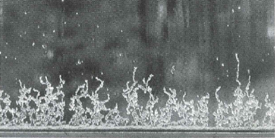
Figure 1.1: Fresh snow falling on the window and forming a rough interface. Extracted from [23].

For instance, one can observe the process of snowflakes falling on the window, sliding down through it and sticking on the first aggregate they have met. Although the whole system is part of our daily experience and seems to be quite “simple”, the generated interface is undoubtedly fascinating - see fig. 1.1. One can notice the presence of large voids, branches and a rough aspect.

Complex interfaces (in the sense of formation, growth and dynamic) are found in the nature from the bacterial growth, spreading of flame fronts, propagation of fluids in porous materials, etc, as well as surfaces made in the lab like those from MBE, eletroconvection and other thin-film deposition techniques [23]. Figure 1.2 displays a Scanning Electron Microscopy (SEM) surface image of Bi film electrochemically grown on a Si substrate. This surface, grown on a two-dimensional substrate, is contrasted with that one formed by snowflakes and presents a rougher aspect which resembles to fern leaves, an example of macroscopic object exhibiting fractal properties. Indeed, interface growth is a close topic to the fractal geometry by Mandelbrot [24] and a concise link between them is established in the chapter 2.

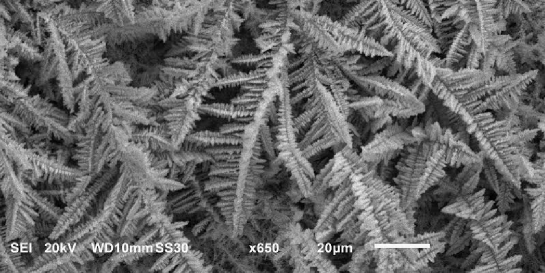
Figure 1.2: SEM image of Bi thin film grown on Si by electrodeposition technique. Courtesy of prof. Renê C. Silva from Universidade Federal de Viçosa, Brazil.

In order to describe the dynamic of growing surfaces which are driven by local processes, continuum growth equations can be proposed. These equations does not take into account the microscopic nature of systems, but only the underlying symmetries and relevant relaxation processes that rule the dynamic at a coarsening-grained level and in a hydrodynamic limit. Under appropriate scale transformations, some statistical quantities are kept unchanged and define, this way, “critical” exponents. In a successful description, the set of these exponents is related to an Universality Class (UC) in which systems sharing dimensionality and large scale behavior can be grouped.

Among a few UCs theoretically predicted, the most remarkable one is that of Kardar-Parisi-Zhang (KPZ) [25]. It has became a celebrated UC because: 1- its continuum growth equation, which is non-linear, can be mapped in classical equilibrium problems of the Statistical Physics [26] and in several mathematical motivated ones [27]. 2- In d = 1 + 1 dimensions, important KPZ models as the Single-Step model [28] and the Poly-Nuclear Growth model [29] allowed uncovering a parallel between the (rescaled) height distribution of KPZ interfaces and the famous Tracy-Widow distributions emerging from the Random Matrix Theory [30, 31]. 3 - Ten years later, analytical treatments on the basis of the famous Directed Polymer in a Random Medium (DPRM) model [32, 26] allowed to solve the KPZ(-DPRM) equation [33, 34, 35, 36, 37, 38], in the meantime that experiments carried out by K. Takeuchi and M. Sano [39, 40, 41, 42], regarding the growth of turbulent liquid crystals, have confirmed the analytical findings and suggested new universal KPZ features. Previous experiments concerning on the low combustion of paper [43, 44, 45, 46], and a recent experimental realization on the deposit of colloidal particles at edge of water drops [47] have also enormously contributed to enoble the KPZ_d=1+1 paradigm. Shortly after Takeuchi and Sano experiments [39, 40, 41, 42], numerical models belonging to the KPZ class have supported and, indeed, gone beyond liquid-crystal results [48, 49, 50, 51] filling, finally, the last pieces toward a consistent KPZ_d=1+1 triumvirate.

In d = 2 + 1, the KPZ situation, however, is very different from its lower dimensional counterpart. There are not analytical results and almost one knows about the most important dimension for technological applications comes from numerical results: the scaling exponents [52, 53] and the height [54], squared local roughness [56, 55] and maximal relative height distributions [57] in the steady-state are older examples. Recently, the universality for height distributions in the growth regime has been verified through large-scale simulations [60, 58, 59, 61]. From the experimental side, evidences of KPZ_d=2+1 systems are extremely rare [62, 63] and a long quest to find out one robust realization confirming the KPZ universality beyond scaling exponents has persisted until the beginning of 2014 [64, 65]. In fact, this poverty of experimental evidences has touching all UCs. Several works (see chapter 11 in the Ref. [23] and section 3 in the Ref. [66]) have been reporting exponent values that do not match with anyone known UC. Inevitably, it has created a deep nuisance in the area, suggesting that the theoretical framework as yet is not completed. Advances as the anomalous scaling [67, 68, 69, 70, 71, 72] have shown that some systems are ruled by different exponents at local and global scales and that the analysis of interface fluctuations in the Fourier space are essentials for accessing the true form of the local scaling law [71]. However, in these situations, a larger number of exponents must be found in order to classify the interface dynamic. It makes the work still harder.

From an experimental point of view, there are some basic aspects hampering the association between a two-dimensional growth and its UC. They are listed in the following:

• Difficulty for imaging surfaces and for growing films at long times - Unlike one-dimensional growing interfaces, it is hard recording the time evolution of two-dimensional surfaces during the growth. Thus, in general, ex-situ probe microscopic techniques are used for imaging the interface at discrete growth times. Each growth time corresponds to an one distinct sample produced in the lab, which, depending on the growth technique and on the growth parameters, can take some hours (or even days) to become ready. Because of this procedure, two-dimensional growths are, usually, conditioned to the finite-time growth, instead to the asymptotic-time growth, where the scaling regime of the true UC is expected to emerge.

• Finite-time effects - During the growth, the interface dynamic can suffer a transition, i.e, a crossover. Temporal crossovers can be identified measuring the time evolution of some correlation function, but even in simulations this is not an easy procedure [73, 67, 74, 75]. For instance, studying the growth of SiO₂ on Si by CVD, F. Ojeda et al. [62] have found the true asymptotic scaling regime only for samples grown at the range of $\sim 10^{2}$ to $10^{3}$ min, after two initial crossovers - see fig. 1.3. From this example, it is clear that if the data from an experiment corresponds to a crossover region (very difficult to be detected), the exponent value extracted from there could not match with any universal value. The same can occur when transient anomalous scaling takes place [67]. Both facts are also reasons of why so many experimental works have found exponents which are not theoretically expected.

  

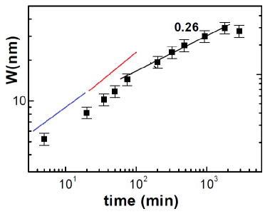
  Figure 1.3: Example of crossovers ocurring in the two-dimensional growth of SiO₂ on Si(001) substrates by CVD. The crossovers are identified by different slopes (blue to red and red to black) at the W(t) scaling in a log $\times$ log plot. The short number of samples makes hard to distinguish different regimes. The value 0.26 refers to the slope of the black curve and was related to the assymptotic scaling regime. Figure extracted and edited from [62].

• The presence of morphological instabilities - When the surface can be decomposed into an array of globules (grains, mounds, etc.), one says there is the presence of morphological instabilities [76]. This feature induces a characteristic length in the system $\zeta$, below which scaling invariance is awaited to be broken. The presence of $\zeta$ modifies local scaling of correlation functions and has led to many equivocated associations between experimental growths and UCs. In particular, non-universal local exponents have been confused with critical ones, as very well explained by Oliveira and Aarão Reis [77, 78]. These studies are addressed in the section 2.3.2.

• Dimensional fragility of the KPZ equation - Concerning on the KPZ class, as theoretically discussed in the ref. [79], a same experimental KPZ_d=1+1 system, when grown in d = 2 + 1 dimensions, might has its exponents deviated from those expected for the KPZ class. This occurs due to the presence of morphological instabilities and non-locality, which are introduced by hand as a perturbation term in the non-linear term of KPZ equation. M. Nicoli et al. have been calling attention for this dimensional fragility as a further obstacle in front of experimental confirmations of KPZ_d=2+1 growth. As extension, one can wonder whether this fragility is really a particular feature of the KPZ equation or can take place in others non-linear growth equations.

Guided by all this experience with two-dimensional experimental systems, as well as the deep knowledge about the KPZ_d=1+1 triumvirate, we have found out the first robust experimental confirmation of the KPZ class in two-dimensional systems, going beyond the standard comparison with exponents [64]. Through a very systematic scheme for investigating the UC of growing films, which advances over the comparison of scaling exponents and provide a reliable way for circumvent out (partially) the obstacles ii-iv), we have confirmed that the growth of CdTe thin films on Si(001) for $T=250\,^{\circ}\mathrm{C}$ belongs to the KPZ class as demonstrated by scaling exponents and universal height distributions, universal squared local roughness distributions and universal maximal relative height distributions [64]. Moreover, this is the first time that it has been experimentally demonstrated the universality of such distributions [64].

As the goal of the present work is twofold (theoretically and experimentally-motivated), we have also studied the effect of the deposition temperature on this novel two-dimensional Kardar-Parisi-Zhang system. We have shown that in the presence of finite-time effects (crossovers and anomalous scaling), scaling exponents are not able to point, in a compelling way, the UC class of the system, mainly due to inexorable experimental obstacles. However, we have shown that this can be circumvented by analysing distributions, which allow us to prove that fluctuations of CdTe interface are described, asymptotically, by the Kardar-Parisi-Zhang equation in a broad range of temperature [80]. Finally, one demonstrates that is possible tunning, experimentally, the KPZ non-linearity through the deposition temperature [80].

The rest of this dissertation is organized as follows. Chapter 2 makes a link between fractals and surface fluctuations, introducing basic statistical tools. Up-to-dated results about the specific subjects of each section can be found diluted along the text and, when indicated, in the Appendix sections. The chapter 3 is deserved for a short review on the Kardar-Parisi-Zhang equation, which includes the mainly ingredients and advances whithin the KPZ theory. In the chapter 4, experimental procedures used during this work are carefully described, as well as the techniques and growth parameters. Chapter 5 presents the first results of this work and exhibits a breaktrough in the context of the two-dimensional KPZ paradigm. On the sequence line, in the chapter 6 one distills the effect of the deposition temperature on the CdTe growth dynamic, and one explores the richnnes emerging from the CdTe system. Finally, in the chapter 7, conclusions and perspectives are drawn with a compreheensive overview of this work, standing out its mainly contributions to the context of kinetic roughening surfaces. Appendix sections cover topics as the random growth equation, the Villain-Lai-Das-Sarma (VLDS) class, etc., the origin and development of anomalous scaling and, finally, an introductory material for young students concerning on the basic physics of crystal growth.

2   Fractals, Scale Invariance and Universality in Interface Growth

In this chapter, a link between growing surfaces and their descriptions, built on the analogy of tools from Statistical-Mechanics of equilibrium phenomena at the criticality is given. Continuum growth equations are discussed and their critical exponents are extracted. Universality is discussed on the theoretical, numerical and experimental approaches.

2.1   From Fractality to the Family-Vicsek Ansätze

A fractal is a complex and irregular object which, under an appropriated scale transformation, (any)one of its parts represent it as the whole. Mountains, clouds, tree leaves and coastlines are some examples of fractals decorating the nature [24]. In a mathematical sense, a fractal is said deterministic if a “zoom” in the system always reproduces exactly the whole object. However, in the nature, one finds statistical fractals. For example, if one compares two snapshots from a mountain at different magnifications they do not overlap but, nonetheless, their statistical properties are the same [23].

A fractal object presents a dilatation symmetry (or homogeneity property) [19]. Statistical homogeneity is described by the condition:

$$f(\varsigma^{\alpha_{1}}x_{1},\varsigma^{\alpha_{2}}x_{2},\varsigma^{\alpha_{3}}x_{3},...)={\varsigma^{\alpha}}f(x_{1},x_{2},x_{3},...),$$ (2.1)

where the object is formed by a set of points $f=f(\textbf{x})$, $\varsigma$ is a scale factor and $\alpha$ is called the Hölder exponent [23].

If ${\alpha_{1}}={\alpha_{2}}=...={\alpha}$ (meaning an isotropic scale transformation) satisfies the eq. 2.1, so one has self-similarity. Otherwise, for anisotropic transformations, one has self-affinity [23, 24].

At a critical point of a phase transition, correlation functions behave exactly as eq. 2.1 [19]. In the Statistical Mechanics language, it implies that the correlation length ($\xi$) diverges and there is no characteristic length in the system beyond system size itself [19]. For non-equilibrium processes such as surface growth, it has been shown that interface fluctuations also behave as those at critical point of a phase transition [23, 19, 66]. In other words, typically, interfaces provided by the nature are fractals in the statistical sense. Let $h(x,t)$ be the height of an one-dimensional interface at the position $x$ at time $t$. Assuming homogeneity, as in eq. 2.1, then:

$$h(x,t)=\varsigma^{-\alpha}h(\varsigma x,\varsigma^{z}t),$$ (2.2)

where z is the dynamic exponent, and $\alpha$, in the surface growth context, is named roughness exponent [23]. Notice that, the dilation symmetry has also been assumed on the temporal axis, which has lead to the z definition. Hence, $\alpha$ and $z$ are characteristic of systems displaying spacial and temporal scaling invariance.

A surface evolving in time is not a deterministic process. The height $h(x)$ at surface is a stochastic variable and have a set of possible outcomes $\{h_{1},h_{2},h_{3}...\}$ distributed from a given probability $P(h)$. In general, the probability for a given height of the interface take the value $h$ is defined as the ratio between the number of occurrences $N_{h}$ of this specific event and the total number $N$ of heights sampled:

$$P(h)=\lim_{N\rightarrow\infty}N_{h}/N.$$ (2.3)

The probability depends on the range ($dh$) in which a value between $h$ and $h+dh$ is measured. So, is more interesting to define the probability density function (pdf) $p(h)\equiv dP(h)/dh$ [19, 81, 82], which must satisfy the normalization requirement:

$$\int_{-\infty}^{\infty}dh\,p(h)=1.$$ (2.4)

A pdf is built up from its moments or cumulants. The nth-moment ($m_{n}$) of a pdf is:

$$m_{n}\equiv\langle h^{n}\rangle\equiv\int_{-\infty}^{\infty}dh\,p(h)\,(h^{n}),$$ (2.5)

where the brackets mean to take the expectation value of the variable $h^{n}$.

The moments are generated through the characteristic function p̃$(k)$, which is the Fourier transform of $p(h)$ [81]. From the logarithm of p̃$(k)$, one defines the nth-cumulant ($\langle h^{n}\rangle_{c}$):

$$\ln\textrm{\~{p}}(k)=\sum_{n=1}^{\infty}\frac{(-ik)^{n}}{n!}\langle h^{n}\rangle_{c}.$$ (2.6)

By expanding the logarithm in the p̃$(k)$ definition and comparing therm by therm with the expansion of p̃$(k)$ in powers of k, one reaches to the relation between the moments and the cumulants [81]. For the first four cumulants, one has, eq. 2.7:

$$\left.\begin{array}[]{p{10cm}}$\langle h\rangle_{c}=\langle h\rangle$,\\ $\langle h^{2}\rangle_{c}=\langle h^{2}\rangle-\langle h\rangle^{2}$,\\ $\langle h^{3}\rangle_{c}=\langle h^{3}\rangle-3\langle h^{2}\rangle\langle h\rangle+2\langle h\rangle^{3}$,\\ $\langle h^{4}\rangle_{c}=\langle h^{4}\rangle-4\langle h^{3}\rangle\langle h\rangle-3\langle h^{2}\rangle^{2}+12\langle h^{2}\rangle\langle h\rangle^{2}-6\langle h\rangle^{4}$.\end{array}\right.$$ (2.7)

The first cumulant is called mean and the second one is variance.

Other important quantities are dimensionless cumulant ratios. In particular, the Skewness S (eq. 2.8) is an indicative of pdf asymmetry [81]. If the expectation value is larger than the more probable one, then $S>0$; otherwise, $S<0$. The Kurtosis K (eq. 2.8) provide information about the “weight” of pdf tails. A symmetric pdf with $K>0$ presents a peak sharper than that from the Gaussian and its tails take longer to fall down. The opposite occurs for $K<0$. By definition, the Gaussian pdf has $S=K=0$. A representation comparing distributions with the same expectation value for different S and K values is shown in the fig. 2.1.

$$S=\langle h^{3}\rangle_{c}/[\langle h^{2}\rangle_{c}]^{3/2}\quad\textrm{and}\quad K=\langle h^{4}\rangle_{c}/[\langle h^{2}\rangle_{c}]^{2}.$$ (2.8)

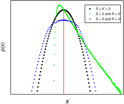
Figure 2.1: Comparison between different distributions having the same expectation value, which is indicated by the solid red line. A curve presenting S < 0 can be obtained performing a parity transformation on the green curve.

The global squared roughness ($w^{2}$) of an interface is defined as the variance of heights composing it. Interestingly, the roughness (or width) is a very important variable from both experimental and theoretical point of view. The electrical conductivity of some thin films, for example, is strongly reduced as rougher is their surface [2, 3, 4]. The importance from the theoretical side will be clear soon. Consider an one-dimensional interface of size $L$. The roughness of such interface at time $t$ reads:

$$w(L,t)=[\langle h(x,t)^{2}\rangle-\langle h(x,t)\rangle^{2}]^{1/2},$$ (2.9)

where the $\langle...\rangle$ refers to a spatial average over the whole system of size $L$.

Now, we can return to the hypothesis made in eq. 2.2. Inserting this equation in the eq. 2.9 and performing algebraic manipulations one finds:

$$w(L,t)=t^{\alpha/z}f(L/t^{1/z}),$$ (2.10)

this equation precede a canonical ansätze in the kinetic roughening theory. Defining the growth exponent $\beta\equiv\alpha/z$, the Family-Vicsek (FV) dynamic scaling ansätze predicts that $f$ asymptotically behaves as $f(u)\sim u^{\alpha}$ for $u\ll 1$ and $\sim$ $const$ for $u\gg 1$ [83]. Leading the ansätze for eq. 2.10, finally, one obtains:

$$w(L,t)\sim\left\{\begin{array}[]{c}t^{\beta},\quad\textrm{for}\quad t^{1/z}\ll L,\\ L^{\alpha},\quad\textrm{for}\quad t^{1/z}\gg L.\end{array}\right.$$ (2.11)

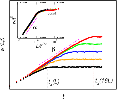
Figure 2.2: Typical time roughness plot (log $\times$ log) during an interface growth for different substrate sizes. The curves refer to substrate of size: black circles (L), orange left triangles (2L), blue up triangles (4L), green diamonds (8L) and red squares (16L). $t_{x}$ indicates the characteristic time in which $\xi_{||}\approx$ substrate size. Inset confirms the FV ansätze, described in eq. 2.11 using the appropriate values for $\beta$ and $z$.

Roughness behavior is sketched in the fig. 2.2. The system roughens as $t^{\beta}$ while the correlations are spreading through it. This is called growth regime. At the time $t_{x}$, the correlation length becomes of the same order of $L$ and a distinct regime is reached: roughness stops growing in time and turns to depend solely on $L$. This is the steady state or saturation regime. Comparing what eq. 2.11 tell us, it is clear to associate $\xi_{||}\sim t^{1/z}$, where $\xi_{||}$ is the parallel correlation length. In inset of fig. 2.2, the FV ansätze is tested, showing remarkable collapse for the curves. We notice that the roughness presents a power-law dependence in space and time, as occurs with the correlation functions in equilibrium critical phenomena. The parallel goes further and, indeed, the “critical” exponents ($\alpha$ and $z$) do not depend on microscopic details of the system under investigation, i.e, there is universality in fluctuations of growing interfaces.

Once the saturation regime depends on $t^{1/z}$ be of the same order of $L$, in experimental situations where $L$ is much larger than the characteristic size of particles constituting the interface, the time required to the system gets into the steady state is hardly achieved. As far as we know, only the evolution of profiles (d = 1 + 1) yielded by slow combustion of paper [43] and the growth (d = 2 + 1) of SiO₂ films by CVD (after 2 days of deposition) have experimentally achieved the stationary state [62].

The FV ansätze has been confirmed in several examples of surface growth such as the propagation of fluid flow in a porous medium [23], paper wetting [23], the growth of turbulent liquid crystals [39, 40, 41], the slow combustion of paper sheets [43, 44] and so on [84]. However, the FV scaling is not the most general one. Indeed, FV ansätze fails for describing local scaling of growth process with anomalous roughening. A detailed description of anomalous scaling is let to the appendix section B.

2.2   Correlation Functions

Correlation functions (CF) play a central role in systems exhibiting criticality (out-of or at equilibrium) because they provide a measurement of the correlation length. They are formed by an operation (sum, product, etc.) involving suitable quantities describing the microscopic state of the system, which are separated by a distance of $\boldsymbol{l}$. Taking an interface of linear size L for instance, one can describe it by its height field $\{h\}_{L}$ or even by its slope field $\{\nabla h\}_{L}$ (of course, in an appropriate coarsening grained level). A CF for an interface growing can, hence, be written as:

$$C_{h}(|\boldsymbol{l}|,t)=\langle[h(\textrm{{x}},t)-h(\textrm{{x}}+\boldsymbol{l},t)]^{2}\rangle.$$ (2.12)

If the system presents translational symmetry, any CF will depend solely on the magnitude of $\boldsymbol{l}$ [19], what is not true for anisotropic systems (see [85] and ref. therein). Furthermore, as discussed at the beginning of this chapter, a CF displays a dilation symmetry at the criticality. Hence, inserting eq. 2.2 in eq. 2.12 and performing algebraic manipulations one reaches to:

$$C_{h}(l,t)=t^{2\alpha/z}f(l/t^{1/z}),$$ (2.13)

where $f(u)$ is the scaling function that, for while, obeys the FV ansätze. $C_{h}$ is often called height-difference correlation function.

Notice that this is the same scaling form obtained for the roughness in the eq. 2.10 with $\beta$ replaced by $2\beta$ and $L$ by $l$. So, at first note, the example showed in the fig. 2.2 is shared by $C_{h}(t)$, but with the growth regime evolving as $t^{2\beta}$. In the same way, one can replace $L$ by $l$ in the eq. 2.9 to obtain a scaling form for the local roughness [$w_{loc}(l,t)$], which is equally a correlation function. From an experimental point of view, it is unpractical changing $L$ of a system in order to extract $\alpha$. Rather, one often uses local measurements, spanning boxes of lateral length $l$ in the interval $[0,L]$ and obtaining the exponent from the hypothesis $C_{h}^{1/2}(l,t)\sim w_{loc}(l,t)\sim l^{\alpha}$. Fig. 2.3 shows a typical behavior of $w_{loc}$ for interfaces in the growth regime.

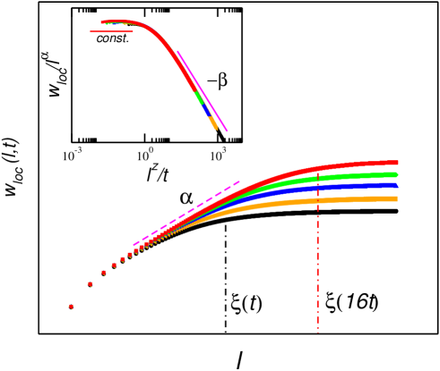
Figure 2.3: Typical local roughness plot (log $\times$ log) for an interface grown at different times. The curves refer to growth times: black circles (t), orange left triangles (2t), blue up triangles (4t), green diamonds (8t) and red squares (16t). Vertical dashed lines indicate the $\xi_{||}$ measured. Inset confirms the FV ansätze, described in eq. 2.11 with L replaced by $l$, and using the appropriate values for $\alpha$ and $z$.

Other important CF is the spatial covariance of heights ($C_{s}$), defined as:

$$C_{s}(|\textbf{l}|,t)=\langle[h(\textrm{{x}},t)h(\textrm{{x}}+\boldsymbol{l},t)]\rangle-\langle h\rangle^{2},$$ (2.14)

where it is straightforward to show that $C_{h}=2w_{loc}^{2}-2C_{s}$.

The covariance $C_{s}(l,t)$ has been computed, in particular, for one-dimensional models belonging to the Kardar-Parisi-Zhang (KPZ) Universality Class (UC) because they are universal and given by the covariance of Airy processes [29, 39, 60] (see fig. 5 in the ref. [39]). Very recently, T. Halpin-Healy and G. Palazantzas have found numerically and confirmed experimentally the universality of the rescaled $C_{s(KPZ)}$ also in 2 + 1 dimensions [65].

Likewise, one can define slope-slope correlation functions using $\nabla$h, instead of h, in the eq. 2.12 and eq. 2.14. Indeed, several experimental studies [16, 86, 64] have used the slope-slope covariance (eq. 2.15) in order to obtain an estimative of $\xi_{||}$.

$$\Gamma(|\textbf{l}|,t)=\langle[\nabla h(\textrm{{x}},t)\nabla h(\textrm{{x}}+\boldsymbol{l},t)]\rangle.$$ (2.15)

An estimative of $\xi_{||}$ can be done measuring either the first zero or the first minimum of the curve [18]. Figure 2.4 shows a plot of a typical behavior of the slope-slope covariance as function of the distance l and time t. The procedure used for estimating $\xi_{||}$ is also indicated, as well as the plot of $\xi_{||}$ as function of the growth time, from where the exponent $1/z$ can be found.

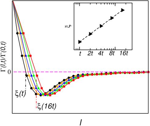
Figure 2.4: Typical normalized slope-slope covariance as function of the distance l and the time t in a linear $\times$ linear plot. Curve colors refer to growth times: black (t), orange (2t), blue (4t), green (8t) and red (16t). Magent dashed line sets $\Gamma(|\textbf{l}|,t)/\Gamma(0,t)$ equal to 0. Vertical dashed lines indicates the position of the estimated correlation length. The inset shows $\xi_{||}$, as function of time in a log $\times$ log plot, from where the exponent $1/z$ can be extracted.

2.3   Continuum Equations and Universality Classes

Let an interface be described by its height field {h(x,$t_{0}$)}, in a appropriate coarsening grained level, and consider there is a known driving force, i.e., there is a far-from-equilibrium situation. An important question concerning on it could be: how does one can describe the height-field evolution of the interface? A priori, the answer does not appear to be reachable because it seems that there is a lack of informations such as: i) the kind of interface (biological, physical, chemical reaction front, etc.) which is being dealt and ii) the specific interactions ruling the dynamics at the microscopic level.

Indeed, an approach to the question from this point of view makes the problem practically intractable. Nevertheless, looking at the macroscopic scales of evolving interfaces, one can glimpse that the collective behavior of them shares many underlying similarities, which does not depend, in fact, of i) and ii). Hence, based on this one could perform a long-wavelength description of the system. Advancing in these thoughts, one can argue that, beyond of the long-wavelength hypothesis, the long-time regime is also a necessary condition, since transient (finite-time) behaviors should be avoided. This particular limit of long wavelengths and long times is called hydrodynamic limit by analogy to the Navier-Stokes equation for a fluid of particles [19].

Guided by these ideas, one can build general equations for describing the height-field evolution of growing surfaces, with the form:

$$\partial_{t}h(\textbf{x},t)=F+\Theta(\textbf{x},\{h\},t)+\eta,$$ (2.16)

with F being the average number of particles per unit time arriving at the interface, the called driving force. Now, one must account that this arriving process is stochastic, and the therm $\eta$ is inserted in the equation for capturing this feature. Regarding $\eta$, one has:

• If the active zone (interface front) advances onto an inhomogeneous medium as a porous substrate or a paper sheet, the relevant noise in the process is static and changes point to point in the medium. This is called of quenched noise, once $\eta=\eta(\textbf{x},h)$. If only the quenched noise is present, the growth of the interface has a deterministic evolution. However, the thermal noise, which is always present in experiments, destroys this determinism.

• Beyond of thermal noise, when an interface grows by receiving particles from an external flux, the so called shot noise is also present and plays the crucial role on the dynamic. This noise comes from the inherent randomness occurring in the deposition process. Assuming there is no preferential area onto the substrate for receiving molecular flux, one has that $\langle\eta(\textbf{x},t)\rangle=0$ with the spatial-temporal covariance given by:

  $$\langle\eta(\textbf{x},t)\eta(\textbf{x'},t^{\prime})\rangle=2D\delta^{d_{s}}(\textbf{x}-\textbf{x'})\delta(t-t^{\prime}),$$ (2.17)

  where $\sqrt{D}$ is the amplitude of the white noise.

Now we turn the attention to the forms which the functional $\Theta(\textbf{x},\{h\},t)$ can assume supposing that the dynamic of the interface is ruled by local processes. As an underlying hypothesis, descriptions of a physic fact can not depend on the origin of its observation $\overleftrightarrow{S}=(t_{0},\textbf{x},h_{0})$. Thus, spatial and temporal translations must be satisfied by the eq. 2.16. It rules out from the functional explicit terms involving $t^{n},\textbf{x}^{m}$ or $h^{m}$, where $m\in\mathbb{R^{*}}$. Moreover, as the growth does not make distinction between “right”- and “left-handed”, the eq. 2.16 must also be invariant under spatial parity transformations with respect to the x axis. These hypothesis reduce the allowed terms in $\Theta$ to combinations of even derivatives such as $(\nabla^{2n}h)(\nabla h)^{2p}$, with $n,p\in\mathbb{N}$.

In a general picture, our considerations until here have led us to consider:

$$\partial_{t}h(\textbf{x},t)=F+a_{1}\nabla^{2}h+a_{2}\nabla^{4}h+...+b_{1}(\nabla h)^{2}+b_{2}(\nabla h)^{4}+...{}$$

$$+c_{11}(\nabla^{2}h)(\nabla h)^{2}+...+c_{np}(\nabla^{2n}h)(\nabla h)^{2p}+\eta,$$ (2.18)

where $a_{i}$, $b_{i}$ and $c_{np}$ are appropriate quantities making the eq. dimensionally consistent.

As we are interested in the hydrodynamic limit, derivatives of higher order are irrelevant to the asymptotic scaling behavior (see ref. [23] pag. 49). Thus, the simplest general equation involving these terms reads:

$$\partial_{t}h(\textbf{x},t)=F+a_{1}\nabla^{2}h+b_{1}(\nabla h)^{2}+c_{11}(\nabla^{2}h)(\nabla h)^{2}+\eta,$$ (2.19)

As we shall see, important continuum growth equations are encoded in the equation 2.19. Nevertheless, there are also others important growth equations that call for a physically-motivated term which makes appear higher derivatives of $h$. In the following section we discuss this subject in details.

2.3.1   Edwards-Wilkinson and the Linear-MBE equation

The Edwards-Wilkinson (EW) equation (eq. 2.20) was proposed in 1982 for describing the sedimentation of granular particles [87]. The equation preserves parity symmetry in the growth direction with respect to the mean height, leading the height pdf to has $S=0$. This particular symmetry rules out even powers of $h$ such as $(\nabla h)^{2n}$ and, in accordance with the general eq. 2.19, it reads:

$$\partial_{t}h(\textbf{x},t)=\nu\nabla^{2}h+\eta(\textbf{x},t),$$ (2.20)

where $\nu\equiv a_{1}$ is a quantity of dimension $[m^{2}/s]$ in the S.I. convention.

The growth average velocity of the interface $v\equiv\langle\partial_{t}h\rangle=Ft$, once $\langle\nabla^{n}h\rangle$ vanishes for periodic bound conditions. The eq. above is written at the referential of the mean height, avoiding the explicit dependence on the flux term and setting $v=0$.

Physically, the laplacian term acts as a conservative smoothing mechanism redistributing the irregularities on the interface, while maintaining the average height unchanged (see pag. 50 in the ref. [23] for a geometric interpretation).

Due to the linear character of this equation, critical exponents can be found straightforwardly by rescaling or by Fourier transform methods. As a prototype case, we shall find exponent values by applying rescaling tools on a general linear equation obtained replacing $2$ by $2n$ on the nabla operator in the eq. 2.20. The method by Fourier transform can be found in details in the pag. 173 of the Ref. [84].

Rescaling: Suppose a rescaling as $\textbf{x}\rightarrow\varsigma\textbf{x}$, $t\rightarrow\varsigma^{z}t$ and $h\rightarrow\varsigma^{\alpha}h$. Inserting in the eq. 2.20 with $2$ replaced by $2n$ on the nabla, one has:

$$\varsigma^{\alpha-z}\partial_{t}h=\nu\varsigma^{\alpha-2n}\nabla^{2n}h+\eta(\varsigma\textbf{x},\varsigma^{z}t),$$ (2.21)

where, using the noise covariance definition (eq. 2.17) and the delta function properties $\delta^{d_{s}}(\varsigma\textbf{x})=\varsigma^{-d_{s}}\delta(\textbf{x})$, one can rewrite the rescaled noise in the expression above by $\varsigma^{(-z-d_{s})/2}\eta(\textbf{x},t)$. Now, assuming scale invariance, one finds the critical exponents (valid for $n\geq 1$):

$$\alpha=\frac{2n-d_{s}}{2}\qquad and\qquad z=2n.$$ (2.22)

The EW eq. is recovered for $n=1$, which yields $\alpha=(2-d_{s})/2$ and $z=2$. In particular, for $d_{s}=2$, one obtains $\alpha=0$ and $\beta=0$ meaning that in the eq. 2.11 the roughness exhibit a logarithm dependence on $t$ and on $L$. The set of exponents $\alpha=\alpha(d_{s})$ and $z=2$ compose the so called Edwards-Wilkinson Universality Class, well described in the hydrodynamic limit by the EW equation. A famous numerical model belonging to the EW class is the Random Deposition with Surface Relaxation (RDSR) proposed in 1986 by Family [88], where the deposited particles are allowed to diffuse at surface until reaching the local lowest height. Experimental evidences of surfaces belonging to the EW class, in turn, are very rare. As far as we are concerned, the EW universality has only been found in the growth of W multilayers on Si by magnetron sputtering [89, 90] and in the sedimentation process of SiO₂ nanospheres [91].

Returning to eq. 2.22, if one sets $n=2$ one obtains the exponents for the famous growth equation known as linear-MBE equation (eq. 2.23), firstly proposed by Wolf and Villain [73] and Das Sarma and Tamborenea [92] for describing the growth of surfaces in which diffusion is the relevant growth mechanism.

$$\partial_{t}h(\textbf{x},t)=-K_{d}\nabla^{4}h+\eta(\textbf{x},t),$$ (2.23)

$K_{d}$ accounts for the strength of the diffusion and has dimension of [$m^{4}/s$].

A derivation of eq. 2.23 from a conservation law is let to the appendix section A.2. Indeed, the deterministic form of eq. 2.23 was known (and was solved) since a long time ago by Herring [93] and Mullins [94] considering the effect of the scale on sintering phenomena and the development of thermal grooves, respectively. Due this, often the stochastic growth equation is called Mullins-Herring equation, instead linear-MBE. However, in this dissertation we will refer to the eq. 2.23 as linear-MBE equation, while its related universality class is being called Mullins-Herring (MH) class.

The critical exponents constituting the MH class are (from eq. 2.22, with $n=2$):

$$\alpha=\frac{4-d_{s}}{2}\qquad and\qquad z=4.$$ (2.24)

Theses exponents were firstly calculated by Wolf and Villain as intention of describing the WV model [73], although, shortly after was found that, actually, the model does not belong to the MH class [75]. Numerical models capturing the diffusion mechanism and truly belonging to the MH class carries the name of Das Sarma, Tamborenea, Ghaisas and J. Kim [95, 96]. A classical review paper on the models can be found in the ref. [97], while a discussion on the WV model is described in the chapter 15 of the ref. [23].

On the experimental side, evidences of MH class have been found in the growth of Si on Si(111) by MBE for $T=275\,^{\circ}\mathrm{C}$ and deposition rate of 7 bilayers/min [98] [scaling was obtained through STM images]; thermal evaporation of amorphous Si on Si(111) substrates at deposition rate of $0.8\pm 0.2$ Å$/s$ [99] [AFM]; the sputter-deposition growth of Pt on glass at deposition rate of 6 Å$/s$ and with the normal substrate aligned about $45\,^{\circ}$ with the target surface normal [100] [STM]; in fluctuations of intra-grain domains of gold electrodeposits grown at 100 $nm/s$ [101] [STM] and in inter-grain fluctuations of $LiCoO_{x}$ thin films grown by rf sputtering, after annealing process [102] [AFM], as well as in the circular growth of cultivated brain tumor [103] [optical microscope].

2.3.2   The Linear Deposition-Desorption-Diffusion equation and Grain Models from Oliveira and Reis

At this point, we could insert together the diffusion and the desorption mechanisms in a continuum growth equation. This makes sense, once specific MBE conditions (very high deposition temperature and/or low supersaturation) can lead the growth to depend sensitively on both processes. Deposition occurs solely if there is a supersaturation ruling the vapor-to-solid phase transition, it means that the difference of chemical potential between the vapor ($\mu_{v}$) and above the solid phase ($\mu(\textbf{x},t)$) is positive. However, when the supersaturation is low [$(\mu_{v}-\mu)\gtrsim 0$], thermal fluctuations make possible, during a characteristic time, a particle to escape from the interface and to move toward the vapor phase. In these conditions, and including diffusion, one has:

$$\partial_{t}h(\textbf{x},t)=F-B[(\mu_{v}-\mu)]-K_{d}\nabla^{4}h+\eta(\textbf{x},t),$$ (2.25)

with B having dimension of inverse of linear momentum.

Inserting $\mu(x,t)\propto-\nabla^{2}h$, one finds the general deposition-desorption-diffusion equation:

$$\partial_{t}h(\textbf{x},t)=F+\nu\nabla^{2}h-K_{d}\nabla^{4}h+B\mu_{v}+\eta(\textbf{x},t),$$ (2.26)

where the ratio $(K_{d}/\nu)^{1/2}$ has dimension of length and, thus, define a characteristic length in the system, $\zeta$.

A trivial rescaling in the eq. 2.26 provides:

$$\varsigma^{\alpha-z}\partial_{t}h=\nu\varsigma^{\alpha-2}\nabla^{2}h-K_{d}\varsigma^{\alpha-4}\nabla^{4}h+B\mu_{v}+\varsigma^{-z-d_{s}}\eta(\textbf{x},t),$$ (2.27)

where for long-wavelength fluctuations ($\varsigma\rightarrow\infty$, $l\gg\zeta$), the laplacian dominates the growth and the exponents are consistent with the EW class. At short-length scales ($\varsigma\rightarrow 0$, $l\ll\zeta$), however, diffusion mechanism overcomes the laplacian effect and the growth is dictated by the linear-MBE equation.

This behavior has been confirmed, for instance, in copper electrodeposition in the presence of 1,3-diethyl-2-thiorea, an organic additive with concentration $x$ ($0.3\leq x\leq 0.4$ $mM$), for low current density $j=0.02$ A $cm^{-2}$ [104]. In this work, the authors have found $\alpha$ and $\beta$ exponents for both regimes, strongly confirming the MH-EW crossover. Notwithstanding, in many studies on the growth of thin films the local roughness is the only curve analyzed, from where $\alpha$ is usually extracted. In particular, when $\alpha\approx 1.00$ a linear-diffusion-dominated dynamic is often suggested, but Oliveira and Reis have demonstrated that this procedure is fail in most of cases [77, 78].

Studying the effect of grains at surface on the local roughness scale, Oliveira and Reis have shown that the general $w_{loc}(r,t)$ plot exhibits two crossovers - see and follow the fig. 2.5. The first regime happens for $r\ll r_{c}$, where $r_{c}$ is the average grain size and is dictated by the exponent $\alpha_{1}$. Length scales between grains $r_{c}\ll r\ll\xi$ define the second regime growing as $w_{loc}\sim r^{\alpha_{2}}$. The second crossover separates correlated from non-correlated regions of the grainy surface.

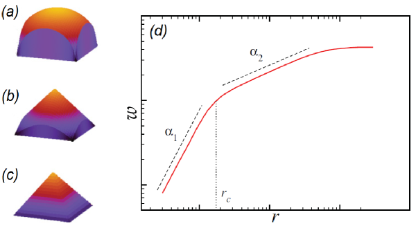
Figure 2.5: Grain of (a) semi-elliptical, (b) conical and (c) pyramidal shapes. (d) General local roughness curve (log $\times$ log) for grainy surfaces. Fig. extracted and edited from Oliveira and Reis [77, 78].

Interestingly, it has been demonstrated that $\alpha_{1}$ has a dependence on the grain geometric shape, on the local correlation function and on the procedure to calculate root-mean-square averages. It implies that $\alpha_{1}$ can not be related to a critical exponent in the sense of capturing universal fluctuations at surface. The geometric interpretation is corroborated with the local roughness curve, where the $\alpha_{1}$ value can change from $0.75$ to $1.00$ for surfaces composed by pyramidal and flat top grains, respectively. The $\alpha_{2}$ exponent, however, keeps constant at the expected UC value related to the model. We recommend the reader take a look at the original papers from Olivera and Reis [77, 78]. Comparison with experiments has been carried out and, just to few some experimental results matching with Olivera and Reis predictions, one finds: the spray pyrolysis growth of ZnO films [105], which gives $0.94\ll\alpha_{1}\ll 0.97$ for high flow rates; the electrodeposition of cooper by Mendez et al. [106], presenting $\alpha_{1}=0.87\pm 0.06$; the sputtering of niquel oxided films ($\alpha_{1}=0.70$) [107]; the growth of bilayers of poly(allylamine hydrochloride) and a side-chain-substituted azobenzene copolymer (Ma-co-DR13), after deposition of 10 or 20 bilayers, giving $\alpha_{1}\approx 0.80$ [108]; and the surfaces of Langmuir-Blodgett films of polyaniline and neutral biphosphinic ruthenium complex, which yields $0.66\ll\alpha_{1}\ll 0.82$ [109].

3   The Kardar-Parisi-Zhang Universality Class: A Brief Historical and State-of-the-Art

This chapter is a natural sequence of the previous one, but due to the richness of the Kardar-Parisi-Zhang equation an entire chapter is deserved to the discussions that one follows. A basic narrative on the motivation, development and current status of this paradigmatic continuum growth equation is presented. We do not have the intention to englobe in this text all what the equation has been demonstrating to offer. Instead, we focus on its scaling properties, on important mappings and on its universal distributions.

3.1   Scaling, Mappings, Height Distributions

The Kardar-Parisi-Zhang (KPZ) equation was proposed in 1986 for describing growing interfaces in which growth in the local normal direction plays a decisive role in the asymptotic dynamics [25]. Based on universality ideas, as well as on existing growth models as the Eden model for cell colony formation [110], and the ballistic deposition model for colloidal aggregates [83, 111], KPZ proposed the simplest nonlinear stochastic equation for describing the height-field dynamic of such interfaces:

$$\frac{\partial h(\textbf{x},t)}{\partial t}=\nu\nabla^{2}h+\frac{\lambda}{2}(\nabla h)^{2}+\eta(\textbf{x},t),$$ (3.1)

$\nu$ represents a “surface tension” due to the geometric interpretation of laplacian term (see ref. [23]), whereas the nonlinear term accounts for the growth in the local normal direction and $\eta$ is the noise.

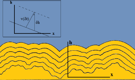
Figure 3.1: Successive profiles for a deterministic KPZ growth with a rough initial condition. Inset indicates how local normal growth occurs. Extracted and edited from [25].

As indicated in the inset of fig. 3.1, when an interface grows laterally, the increment along the $h$ axis ($\delta h$) and the local normal velocity $v$ are related by the Pythagoras’ theorem: $\delta h=[(v\delta t)^{2}+(v\delta t\nabla h)^{2}]^{1/2}$. Inserting the small slope approximation ($\nabla h\ll 1$), one can perform an expansion at the right side of the equation leading to: $\frac{\partial h}{\partial t}\simeq v+(v/2)(\nabla h)^{2}+...$ . Eq. 3.1 is obtained after a transformation to the moving frame ($h\rightarrow h+vt$) and after the relaxation mechanism is inserted. Nonlinear higher-order terms are disconsidered because they go to zero faster than $(\nabla h)^{2}$ in the hydrodynamic limit, as already discussed in chapter 2.

Unlike linear growth equations, the mean interface velocity of the KPZ equation takes the form: $v=Ft+\frac{\lambda}{2}\int_{0}^{L}d^{d_{s}}x\langle(\nabla h)^{2}\rangle$, which is different from zero even when $F=0$. $\lambda$ accounts for this “excess of velocity”. In particular, if $\lambda=0$ one obtains the EW equation (eq. 2.20) and if, additionally $\nu=0$, one finds the Random Growth equation (see appendix section A.1).

The KPZ equation can be easily solved in its deterministic form ($\eta(\textbf{x},t)=0$), which leads to interfaces composed by paraboloid segments resembling dendrites [25], see fig. 3.1 for a typical one-dimensional growth pattern. On the other hand, the stochastic equation (eq. 3.1) has been resisting to a complete analytical handling. Great part of the advances on the solution of the KPZ equation has moved on owing to the arsenal of powerful tools that mathematicians has brought to the field. For instance, analytical models that belong to the KPZ equation as the Single-Step model [28] and the Poly-Nuclear-Growth (PNG) model [29, 112] have, togheter with, the Totally Asymmetric Exclusion Process (TASEP) [113] and the Directed Polymer in a Random Potential (DPRM) [32] (which can mapped onto the height field of a KPZ interface), played a crucial role within the KPZ theory. For this last, at the beginning of this decade, analytical treatments have been achieved for d = 1 + 1 dimensions for different geometries, which in the surface growth context refers to a curved [33, 34, 35, 36], flat [37] and stationary [38] growth Initial Conditions (IC). Solutions of higher dimensions, however, are in a fog of analytical hopes.

Regarding to the KPZ scaling, if one applies, naively, the trivial rescaling used in the section 2.3.1, one obtains three self-inconsistent scaling relations. Arguing that the nonlinear term should dominate the growth in the hydrodynamic limit and applying the rescaling again (without the laplacian term) one finds $\alpha=(2-d_{s})/3$ and $\beta=(2-d_{s})/(4+d_{s})$, whose predictions are quite different from numerical results [26, 114, 49, 48, 115, 52]. Indeed, this procedure is wrong because terms like $\nu,\lambda$ and $D$ do not renormalize independently - being coupled to each other [23]. The correct prediction for KPZ exponents can be achieved using Renormalization-Group techniques and mappings to other problems. Through the $u=-\partial_{x}h$ transformation, the KPZ equation with $\lambda=1$ is mapped in the Burgers’ equation with noise [116], describing the vorticity-free velocity field of a stirred fluid. Additionally, the fact that $\lambda=1$ in the Burgers’ equation points out that we must preserve the scale invariance on the nonlinear term in the KPZ context. This reasoning provides the hyper-scaling relation:

$$\alpha+z=2.$$ (3.2)

This relation is a consequence of the Burguer equation to be invariant under a galilean transformation, $u(x,t)\rightarrow u_{0}+u(x-v_{0}t,t)$, which in turn, leads the KPZ equation to be invariant under a tilting transformation by an angle $\epsilon$:

$$h^{\prime}\rightarrow h+\epsilon x;\quad x^{\prime}\rightarrow x-\epsilon\lambda t;\quad t^{\prime}\rightarrow t.$$ (3.3)

The fluctuation-dissipation theorem [23] reveals that, at the steady state (for $d=1+1$), $\nabla h$ follows a Gaussian distribution likewise the position of a particle in a Brownian motion and brings out $\alpha=1/2$. Together with eq. 3.2, this implies $z=3/2$ and $\beta=1/3$, in agreement with previous [114, 26] and recent [49, 48, 117, 51] numerical models belonging to the KPZ universality class.

The concept of “universality beyond exponents” has initiated in the classical paper from Krug, Meakin and Halpin-Healy, back to 1992’s [114]. In that work, by using the so-called “Krug-Meakin toolbox” [118, 119], it was possible to write universal amplitudes in terms of model parameters, namely, $A\equiv f(D/\nu)$ and $\lambda$, which can be easily obtained in simulations [114, 49, 51, 65]. Almost 10 years after this imporant result, Johansson studied a model for which several probabilistic interpretations can be given [28]. Among them, an interpretation in terms of the one-dimensional TASEP (in turn mapped onto the interface fluctuations of the Single-Step model) allowed to show that the pdf of a random amplitude ($\chi$) related to the height field of the Single-Step model (eq. 3.4) is the celebrated Tracy-Widom (TW) distribution [30, 31], emerging from the Random Matrix Theory context.

$$h(t)\simeq v_{\infty}t+sign(\lambda)(\Gamma t)^{\beta}\chi.$$ (3.4)

Here $v_{\infty}$ is the asymptotic velocity of the interface [$v_{\infty}\equiv lim_{t,L\rightarrow\infty}\langle\partial_{t}h\rangle$], $sign(\lambda)$ is the signal function, $\Gamma\equiv aA^{1/\alpha}|\lambda|$, with $a$ being a constant and $A\equiv f(D/\nu)$ in d = 1 + 1 dimensions (see Ref. [114]).

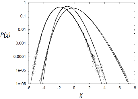
Figure 3.2: Universal distributions obtained by Prähofer and Spohn in the Ref. [29]. From left to rigth: universal pdfs (solid lines) for $\chi$ under curved, flat and stationary self-similar growth, respectively. Symbols refers to simulations of the PNG model. Figure extracted from the ref. [29].

Shortly after, Prähofer and Spohn [29, 112] unveiled a dependence of p($\chi$) on the geometry (IC) of the growth. By using the mapping of the PNG model onto random permutations, they showed that $h(x,t)$ corresponds to the length of the longest increasing subsequence of such permutation, which in turn, is distributed according to: 1) the Gaussian Orthogonal Ensemble (GOE) TW distribution for a flat IC; 2) the Gaussian Unitary Ensemble (GUE) TW, if the growth starts from a seed and develops a curved interface; and 3) the Baik-Rains $F_{0}$ limiting distribution [120] for a steady-state IC. Figure 3.2 shows p($\chi$) for different growth geometries and for stationary initial configuration calculated from the PNG model and compared to the respectives GUE, GOE and $F_{0}$ distributions [29].

A decade later the results of Prähofer and Spohn [29, 112], analytical solutions on the one-dimensional KPZ(-DPRM) equation, already cited above, have confirmed the limiting distributions of $\chi$ as GUE for curved growth [33, 34, 35, 36], GOE for flat growth [37] and $F_{0}$ for the stationary initial condition [38]. Moreover, finite-time corrections were found, suggesting new universal KPZ features such as a shift in the mean converging to GOE (GUE) values as $t^{-\beta}$. It was also demonstrated that the limiting processes, giving the one-dimensional heigth profiles of a KPZ interface, are dictated by the Airy₁ [121, 122, 123] and Airy₂ [124, 123] processes for flat, and curved growing, respectively.

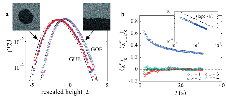
Figure 3.3: Results for turbulent liquid crystals extracted and edited from Takeuchi [40]. (a) Histogram of rescaled local height $\chi\equiv h-v_{\infty}t/(\Gamma t)^{1/3}$. The blue and red solid symbols show the histograms for the circular and flat interfaces, respectively. Dashed and dotted curves show GUE and GOE TW distributions. (b) How $\chi$ cumulants approach to the GUE values. Inset shows the mean shift decaying as $t^{-1/3}$. The same behavior is shared by the flat case (not shown here).

Simultaneously, experiments of unprecedented statistics on turbulent liquid crystals performed by K. Takeuchi and M. Sano [39, 40, 41, 42] have confirmed carefully great part of the predictions cited above and have given to the KPZ_d=1+1 theory a reliable reality beyond mathematical, numerical, and few experimental realizations constrained to exponent results [125]. By using the Krug-Meaking toolbox for unearthing non-universal parameters $A$ and $\lambda$, K. Takeuchi and M. Sano calculated the pdf of the $\chi$ variable, defined according to the KPZ ansätze (eq. 3.4) as $\chi\equiv(h-v_{\infty}t)/(\Gamma t)^{1/3}$. In the fig. 3.3(a) one can see a comparison between the experimental p($\chi$) obtained in that work for both curved and flat cases and the GUE and GOE distributions [40]. Wonderfully, a great accordance was obtained apart from a slight shift at mean of the distributions. In fact, in the figure 3.3(b) the shift at the mean is also calculated, suggesting that it decays as $\sim t^{-1/3}$, while the shift for higher cumulants vanishes quickly.

Remarkable experiments on colloidal particles deposited at the edge of evaporating drops were also able to confirm the “KPZ universality beyond exponents”, where curved deposits of particles slightly anisotropic following the GUE-TW distribution were found [47]. Analytical and experimental results have been reinforced by numerical ones [50, 48, 49, 51], which have filled the last pieces toward a robust and consistent KPZ_d=1+1 triumvirate.

The KPZ_d=2+1 situation is very contrasting with its one-dimensional counterpart and almost all one knows about the most important dimension for applications has come from simulations and, very recently, from some remarkable experimental efforts [64, 65]. Best estimates for scaling exponents indicate that [52, 53, 58]:

$$\alpha\approx 0.393\qquad\beta\approx 0.242\qquad 1/z\approx 1.607.$$ (3.5)

The universality of dimensionless cumulant ratios of $h$, namely, the skewness and kurtosis (eq. 2.8) were firstly calculated numerically at the stationary state, where their values were proved to be universal (see Ref. [54] and references therein). The universality in the growth regime, although glimpsed in the Ref. [134], only was convincingly demonstrated in the year of 2012. Through large-scale simulations, T. Halpin-Healy [58, 59] and T. J. Oliveira et al. [60] have uncovered the existence of geometry-dependent KPZ universal height distributions at the growth regime, higher dimensional GOE- and GUE-TW counterparts, lying in the heart of KPZ_d=2+1 universality. Although the exact forms of these distributions are not known, Oliveira et al. have demonstrated that rescaled height pdf’s can be well fitted by generalized Gumbel distributions [126] (see the definition in the section 3.3) with parameters m = 6 and m = 9.5 for flat and curved cases, respectively. Moreover, as in d = 1 + 1 dimensions, results from the T. J. Oliveira et al. study [60] have supported a generalization of the KPZ_d=2+1 ansätze (eq. 3.4) inserting appropriate finite-time corrections. The final KPZ ansätze reads:

$$h(t)=v_{\infty}t+sig_{\lambda}(\Gamma t)^{\beta}\chi+\eta_{p}+\zeta_{p}t^{-\gamma_{p}}+...,$$ (3.6)

where $\eta_{p}$, $\zeta_{p}$ and $\gamma_{p}$ are non-universal parameters [127, 61]. The values for these model-dependent parameters can be found in the references [114, 49, 48, 61, 51] for d = 1 + 1, and [58, 59, 60, 61] for d = 2 + 1. Deserving much more attention, the universal-KPZ values for the cumulants of height distributions are grouped in the tables 3.1 and 3.2.

	GOE	GUE	Baik-Rains
$\langle\chi\rangle_{c}$	-0.76007	-1.77109	0
$\langle\chi^{2}\rangle_{c}$	0.63805	0.81320	1.15039
|S|	0.2935	0.2241	0.35941
K	0.1652	0.09345	0.28916

Table 3.1: Universal KPZ values for cumulants of height distributions in d = 1 + 1 [29].

	Flat	Curved	Flat-Growing	1D Groove	Stationary
$\langle\chi\rangle_{c}$	-0.75(5)	-2.3(1)	-2.4(2)	-1.47(2)	==
$\langle\chi^{2}\rangle_{c}$	0.23(1)	0.33(2)	0.34(2)	0.249(4)	0.46(2)
|S|	0.423(7)	0.33(1)	0.33(2)	0.396(7)	0.244(8)
K	0.344(9)	0.212(7)	0.21(2)	0.31(2)	0.176(4)

Table 3.2: Universal KPZ values for cumulants of height distributions in d = 2 + 1 dimensions for Flat case [58], Curved [59], flat-growing [61], 1D groove initial condition [59] and Stationary state [59].

As a final remark on KPZ height distributions, we point out that studying KPZ growth on enlarging flat substrates, Carrasco et al. have revealed that the Tracy-Widom distributions and the Airy processes (as well as their (2 + 1)-dimensional analogs) do not depend on the interface macroscopic curvature, but actually on the inflation of the lattice metric on the active zone [61]. Furthemore, in the search for an upper critical dimension in KPZ class, Alves et al. [128] have confirmed that the KPZ ansätze is valid up to d = 6 + 1 dimensions, at least for the Kim-Kosterlitz model [129].

3.2   Universal Squared Roughness Distributions

In 1994, investigating the old problem of random-walk interfaces, Fóltin et al. [130] showed that the squared roughness pdf [$P(w^{2})$] of such interface, at steady state, behaves as:

$$P({w^{2}})=\frac{1}{\langle w^{2}\rangle}\Phi({w^{2}}/{\langle w^{2}\rangle})$$ (3.7)

where $w^{2}$ is the squared global roughness (eq. 2.9) of the interface, $\Phi(u)$ has a closed form and is also an universal scaling function. Indeed, its universality was confirmed by numerical simulations of EW and KPZ models, and have emphasized the power of that distribution for accessing the UC of a given growth process, once it presents a weak dependence on finite-size corrections.

In the same year, Plischke et al. [131] extended theses studies for curvature-driven interfaces and have reinforced the validity of the eq. 3.7 as well as the universality of $\Phi$, which in this case has a different form from that for Gaussian interfaces. Following the same idea, Rácz et al. [55] calculated numerically $P(w^{2})$ for several UCs in d = 2 + 1 dimensions and exposed that, unlike the lower-dimensional case, $\Phi_{EW}$ and $\Phi_{KPZ}$ are different, being the first a Gaussian and the last one marked by a slow decay in the rigth tail. $\Phi_{MH}$ and $\Phi_{VLDS}$ also exhibited remarkable differences between each other. In the same paper one finds a “recipe” of how comparing $\Phi$, for a given UC, with the ones obtained in experiments. The recipe consistes in divide the surface into boxes of lateral size $l\ll\xi_{||}$ inside which $w^{2}$ should be calculated to yield a large ensemble. On the other hand, $l$ must also be larger than characteristic sizes at surface such as grains, mounds, etc.

The Squared Local Roughness Distributions (SRLDs) have been used in signal analysis [132] and in issues about the upper critical KPZ dimension [56] because they are considered one of the most suitable ways for accessing the UC of a growth. For instance, in a very interesting study [133], Aarão Reis analyzed the rescaled distribution $\Phi$, at mean null and unitary variance, (call it $\Psi$, defined as in the eq. 3.8) for one- and two-dimensional models belonging to the KPZ and VLDS classes.

$$P(w^{2})=\frac{1}{\langle w^{2}\rangle_{c}^{1/2}}\Psi\Big{(}\frac{w^{2}-\langle w^{2}\rangle}{\langle w^{2}\rangle_{c}^{1/2}}\Big{)}.$$ (3.8)

Aarão Reis have confirmed that, in d = 2 + 1, $\Psi_{KPZ}$ presents a stretched exponential in the rigth tail as approximately $exp(-x^{0.8})$ [133] - see figure 3.4(a). This form is contrasted with those from $\Psi_{EW}$, which is Gaussian, and with the simple exponential decay of $\Psi_{VLDS}$ and $\Psi_{MH}$. Even the last ones can be easily distinguished in the $\Phi_{VLDS}$ and $\Phi_{MH}$ scaling, as exemplified in the inset (B) of fig. 3.4(a). A subsequent work from Paiva $\&$ Aarão Reis [134] brought out $\Psi_{KPZ}$ in the growth regime presenting a similar decay at the right tail as shown in the fig. 3.4(b). This feature has been suggested as an universal and distinct KPZ landmark [134] and has been confirmed experimentally in the growth of CdTe [64] and oligomer [65] thin films.

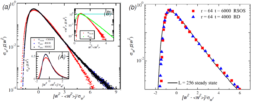
Figure 3.4: (a) The main plot exhibits the contrasting form of universal $\Psi$ distributions for the VLDS and KPZ classes calculated from the CRSOS ($L=64$), RSOS ($L=256$) and RSOS2 ($L=128$) models at the stationary state, for $d=2+1$, according to the ref. [133]. The insertion (A) reinforces the difference between $\Psi_{VLDS}$ and $\Psi_{KPZ}$ near of the peak, whereas inserts (B) shows the constrast between $\Phi_{VLDS}$ and $\Phi_{MH}$. (b) Comparasion between $\Psi_{KPZ}$ calculated from the steady state (solid line) and from two-dimensional RSOS and BD models in the growth regime, for a “box” of lateral size $r=64$. Results in (a) and in (b) can be found in the references [133] and [134], respectively. Theses results were kindly provided by Prof. Aarão Reis.

3.3   Universal Maximal Relative Height Distributions

Extreme-value statistics (EVS) play an important role in systems where rare events have drastic consequences such as floods, internet failures, stock market crashes as well as in important technological applications [126, 135, 136, 137, 138, 57]. For instance, the onset of a breakdown of corroded surfaces is determined by their deepest (or weakest) point, whereas in batteries the highest point of the metal surface reaching the opposite metal surface is responsible by the beginning of a short-circuit [135]. A well-known probability function in the EVS context is the called Gumbel’s first asymptote, being the distribution of the nth value among $N$ independent (uncorrelated) random variables [126]. The Gumbel pdf, $G(X;m)$, of the variable $X$ is defined as:

$$G(X;m)=\frac{m^{m}b}{\Gamma_{f}(m)}\exp[-m(z_{X}+\exp(-z_{X}))],$$ (3.9)

where $m$ is a parameter, $b=\sqrt{\psi_{1}(m)/\langle X^{2}\rangle_{c}}$, $z_{X}=b(\langle X\rangle-X+s)$, $s=[ln(m)-\psi_{0}(m)]/b,\Gamma_{f}(X)$ is the gamma function, and $\psi_{k}(X)$ is the polygamma function or order k[126, 57].

Early studies on EVS applied on growing interfaces focused on the steady state of linear (EW) equations [135, 136, 137]. Through maximal relative height ($m^{*}$) analysis, defined as the difference between the largest height minus the average height of the surface, it was shown that in the stationary regime $m^{*}$ scales likewise the global roughness (this result is valid only for the one-dimensional case) [135] and that its universal distribution, $P(m^{*})=L^{-1/2}f(m^{*}L^{-1/2})$, is dictated by the Airy distribution function, $f(x)$, whether periodic boundary conditions are used [137].

Interestingly, even for strongly correlated systems such as two-dimensional EW interfaces at steady state, it has been shown that $P(m^{*})$ can be very well fitted by the Gumbel, with a non-integer value, n = 2.6(2) in this case [138]. A numerical work has brought theses discussions for KPZ and VLDS two-dimensional surfaces [57]. It was confirmed the universality for either the scaled maximal- or minimal-relative height distributions (MRHDs), depending on the relevant nonlinear term signal. Moreover, the remarkable contrast between the right tail decay from MRHD_KPZ (simple exponential) and MRHD_VLDS (Gaussian) and the very weak finite-size effects affecting these distributions have suggested an alternative way for accessing the UC of a given growth. Our experimental results have been the first confirmation of such universality of this distribution in the KPZ_d=2+1 context.

4   Material and Experimental Methods

In this chapter a short review on the experimental techniques used along this work is given. Details on growth parameters and on the experimental methodology is discussed in details.

4.1   Hot Wall Technique

Hot Wall Epitaxy is a well-established technique based on thermal evaporation developed at the end of the 1970’s which has been used for growing high-quality films from II-VI, IV-VI and also III-V compounds [139, 9]. The great difference between a simple thermal evaporation system and a HWE one consists the presence of a heated liner (hot wall). This liner serves as a guide for the vapor beam to flow from the source towards the substrate, ensuring low material loss and growth conditions as near as possible of the thermodynamic equilibrium.

HWE systems share the same basic structure (see fig. 4.1), but they can be modified depending on the particular growth necessities (see [139] for different HWE forms). In general, there are tree resistances windings at quartz tube to heat the substrate, the source and the wall, independently. It guarantees that the temperature displayed at the controller is always being measured at the same referential, beyond of making the system’s calibration to be very reliable. HWE works in high vacuums ($\approx 10^{-7}$ Torr), providing a relatively clean environment for the growth [140, 141, 9]. Substrate position can work as a lip for the wall or can be slightly inserted above it when a shutter is available.

As a very simple technique, HWE is unsuitable for doping, for growing compounds with very different vapor pressures and it also does not allow in-situ measurements. Indeed, these disadvantages turn the HWE use minimized. However, in situations where in-situ measurements are not essential, where the compounds evaporate congruently and do not have high temperature of sublimation, HWE is absolutely one of the most suitable techniques to be employed due to its high reproducibility, wide growth rate range (0.01 - 10 Å/s) [9] and its relative low cost (ownership and maintenance). This is, particularly, the case for the growth of CdTe [9, 10, 140, 141, 16, 142].

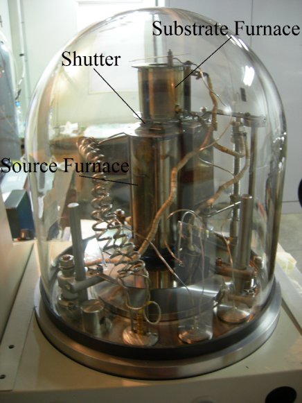
Figure 4.1: Hot Wall system of Epitaxy Laboratory, Physics Departament of the Universidade Federal de Viçosa, Brazil. The legend in the figure shows two furnaces (substrate and source) that work independently and a shutter which allows starting/finishing the growth. The pressure during the growth can reach $\sim 10^{-7}$ Torr.

4.2   Atomic Force Microscopy

After the 1986 year, AFM invention [143] has enormously assisted the surface study in micrometer scale beyond of helping several stages of the thin-film production [4]. As a blind man must use his fingers to feel topographic variations during a Braille lecture, the AFM consists in to obtain morphological data from interactions between a very thin tip (order of $10^{-8}m$ radii) and the sample surface to yield a three-dimensional image. The equipment measures atomic forces via a spring deformation, more known as cantiveler, under which the tip is coupled. On the other cantiveler face, a laser beam is focused and reflected to a photo-diode in order to send electrical signals associated with the cantiveler’s deflection to the controller. A simplified view of most important AFM components is shown at fig. 4.2.

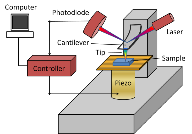
Figure 4.2: Basic scheme of working principles of an Atomic Force Microscope.

Once the electrical signals have arrived at controller, they are translated and sent to the computer to yield a bidimensional profile sketched by the tip. An AFM image can have 1024 x 1024 pixels, which means that there are 1024 bidimensional profiles, each one of them being composed by 1024 equally spaced points. In some AFM systems, the sample is supported by a piezoelectric ceramic which suffers well-behaved subnanometric deformations to move the sample in relation to the tip.

There are two basic AFM measurement modes, namely, contact and tapping. In the former, the tip approaches to the surface until suffer a repulsion force, which causes the tip to bend up. In the tapping mode, however, the tip is set to oscillate near to its natural resonance frequency and gets close to the surface until the oscillation amplitude becomes reduced to a smaller referential value (this occurs at distance between regions of repulsion and attraction). For both modes, the piezo adjusts, through a feedback mechanism, the height axis (z) to hold or the force (contact) or the amplitude (tapping) constant. Then, a surface image is obtained from those z values recorded by the piezo. The choice of which method should be employed depends on the aspects of the studied material (shape, structure, nature) and the kind of results that want to be found (local friction coefficients, phases difference, conductance variations, etc). For instance, biological samples are most suitable for tapping mode once it avoids damage sample and frictional forces, while contact is most suitable for thin films and crystals in general.

Nowadays, AFM is one of the most used techniques for studying surfaces at the submicrometer level. In particular, several works have used AFM images to perform scaling analysis of interfaces, as exemplified by works involving the growth of $SiO_{2}$ by CVD [62], the dissolution of polycrystalline pure iron [86], the amorphous Si by thermal evaporation [98] and Pt sputtered on glass [100].

4.3   Si surface cleaning

Substrate cleaning is the key initial step in thin film and epitaxial growth. In order to obtain flat and contamination-free Si surfaces, several chemical and/or thermal treatments have been proposed since 1980’s [144, 145, 146]. Basically, the aim is to remove the silicon native oxide layer ($\approx 0.7$ nm of thickness) and the hydrocarbon contaminant layer ($\approx 0.2$ nm). The former is usually removed by low-concentration aqueous HF solution [1-10$\%$] using HF and water of high purity, which provide an “ideal” stable monolayer H-terminated Si surface, depending on the aqueous pH concentration [147, 148, 149]. Moreover, aqueous HF solution does not etch the bare Si surface itself, preserving a Si smooth morphology (typically, $\approx 0.2$ nm of roughness [146]). Whereas some works stress the necessity of removing reminiscent hydrocarbon impurities [144, 145], X-ray photoelectron spectroscopy (XPS) measurements show that 1.5% HF-treated Si surfaces present a very low concentration of $O$, $F$ and $C$ [146]. Moreover, the H-terminated surface obtained by this process proved to be very stable against the oxidation in air. In particular, this cleaning procedure has been used for growing epitaxial CdTe QD’s on Si(111) [9]. Another approaches as the degreasing by acetone, ethanol and deionized (DI) water followed by repeatedly boiling in HNO₃, dipping in HF, rinsed with DI water and dried with N₂ also are commonly used [140].

4.4   CdTe thin films: Cleaning, Growth and Characterization

In this work, p-type Si(001) substrates of dimensions $10.0$ mm $\times$ $10.0$ mm $\times$ $0.3$ mm were dipped 2 minutes into an aqueous HF($2\%$) solution prepared with DI water. This time has been checked to be able of removing completely the Si native oxide layer [146]. At the sequence, Si surfaces were exposed to $N_{2}$ air jet just to remove any reminiscent droplet on the surface, once after HF treatment the surface becomes largely H-terminated. The treated surfaces were immediately inserted into the HWE chamber, inside which a high vacuum was performed. There was no any heating treatment before or after the growth.

The HWE system used in this work is composed by two independent furnaces (source and substrate), separated by a shutter and a wall of 7 cm, as shown in the fig. 4.1. The deposition occurs at pressures $\approx 10^{-7}$ Torr, obtained by a diffusion pump system, while the source temperature can be controlled from $400$ to $520\,^{\circ}\mathrm{C}$, producing growth rates between ($\approx 0.01$ and $2.5$ Å/s). The temperature of the substrate (more known as the deposition temperature) can be varied from 150 up to $550\,^{\circ}\mathrm{C}$.

Solid CdTe (99.999%) has been used as source material. The temperature of the source was fixed at $520\,^{\circ}\mathrm{C}$ yielding a deposition rate $F=2.2\pm 0.3$ Å/s for deposition temperatures set at 150, 200, 250, and $300\,^{\circ}\mathrm{C}$. For each deposition temperature, the growth time ($t$) was varied from 15 to 240 min in a geometric progression sequence of ratio $2$, providing thicknesses ($th$) from approximately $0.20$ up to $3.5$ $\mu m$. The $th$ and the growth rate $F$ were determined post-growth using a XP1 - AMBÍOS contact profilometer and a ContourGT-K BRUKER optical profilometer.

Surface characterization was performed in air by ex-situ AFM. We have used an Ntegra Prima SPM working in contact mode. Different kinds of Si tips were used in order to check the reliability of data. All of them were used in the statistical analysis. The frequency of the AFM scan was kept near of 1.5 lines/s during acquisition of the images, but we have also confirmed that the frequency does not affect the results as far the frequency is not set at very high values as $\gtrsim$ 4.0 lines/s. Surface topography of 3 to 10 different regions near of the center film of each sample was scanned producing images of $10$ $\mu m$ $\times$ $10$ $\mu m$ with $1024$ $\times$ $1024$ pixels. This size was chosen so that morphological properties in domains smaller and larger than the averaged grain size could be simultaneously investigated. However, different sizes of scanning were carried out, namely, $1$ $\mu m$ $\times$ $1$ $\mu m$, $30$ $\mu m$ $\times$ $30$ $\mu m$ and $100$ $\mu m$ $\times$ $100$ $\mu m$ to guarantee the validity of data in different scales. For all images a flatten’s correction of second order was performed to correct the sample misalignment and the piezo scanner error.

5   RESULTS: Uncovering the KPZ Universality in CdTe Thin Films

The results contained in this chapter are related to films grown at a particular deposition temperature, namely, T = $250\,^{\circ}\mathrm{C}$. Here we develop a noveil procedure to distill the Universality Class (UC) of a given growth, which consists in to: i) perform a visual-AFM investigation of the interfaces fluctuations focusing on the dynamic of superficial structures whose length is characteristic; ii) relate it to a deep local scaling analysis; iii) add on the results coming from the global scaling and, finally, iv) to find and/or to confirm the UC of the growth by using universal distributions. As we will be seen below, through this scheme we were able to find the UC of CdTe thin films, in the meantime that one has been experimentally demonstrated the universality of KPZ_d=2+1 distributions.

5.1   Semi-Quantitative Morphological Analysis

At first, it is important to observe how the morphology evolves as function of the growth time in a semi-quantitative fashion. Figure 5.1 shows $10\times 10$ $\mu m$ AFM images for all available times. The images depicted are those which better represent typical behavior over all regions scanned.

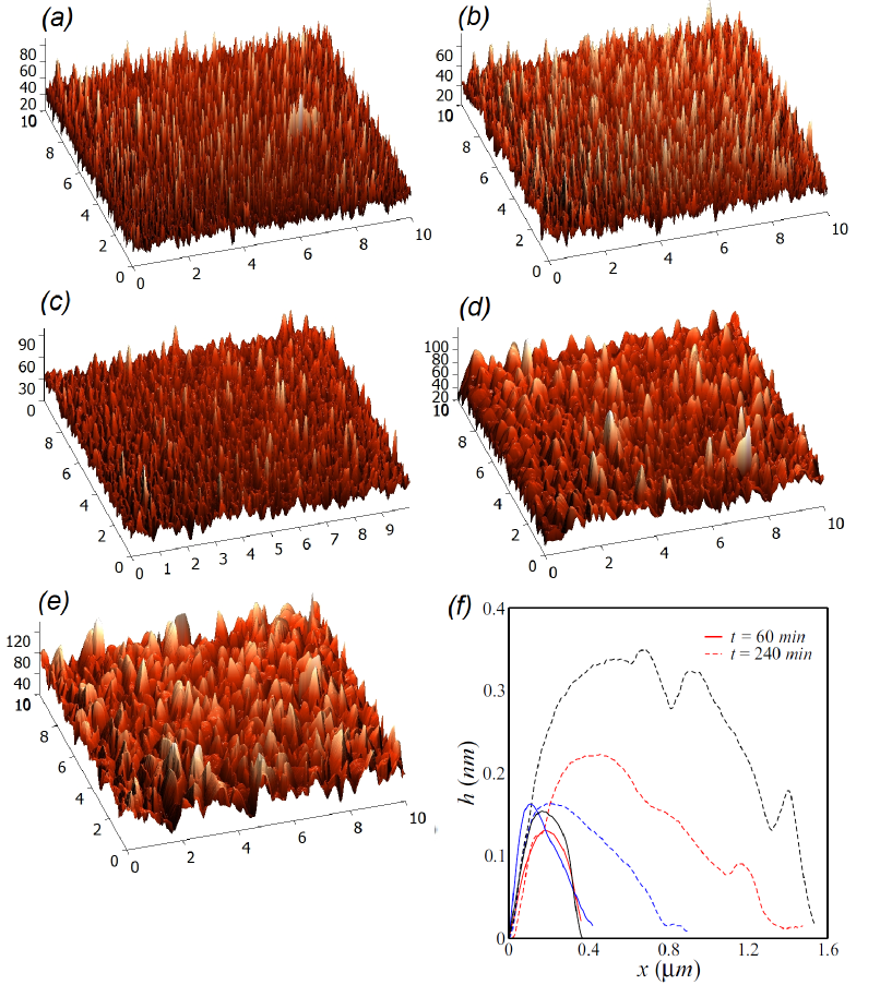
Figure 5.1: AFM images [$10\times 10$ $\mu m$; height scale in nanometers] for CdTe thin films grown at T = $250\,^{\circ}\mathrm{C}$. (a) - (e), Interfaces grown by 15, 30, 60, 120 and 240 min, respectively. (f) Typical grain’s shape present at the interface for t = 60 min (solid lines) and t = 240 min (dashed lines).

At initial times (figures 5.1 (a) and (b)), the surface is dominated by a large number of grains with well-defined “sharp” shape, which present a very high aspect ratio ($\Omega$), defined as the ratio between the crystallite height and the characteristic length of its base (the average grain width - $\zeta$). Roughly, one observes $\zeta\ll 0.5$ $\mu m$ for $t=15$ and $30$ min, whilst the vertical bar decreases from $80$ $nm$ to $60$ $nm$. Consequently, $\Omega$ seems to decrease in this interval. At the subsequent time, one can see a surface composed by fewer, but larger grains ($\zeta\approx 0.5$ $\mu m$) surrounded by a crowd of smaller sharp grains. It is not difficult to see that $\Omega$ has decreased once again. Remarkably, for the last two surfaces showed in the figures 5.1 (d) and (e), one notices the presence of grains with larger basis, in particular, $\zeta\lesssim 0.8$ $\mu m$, and having a smoother top, contrasting with those previous conical-like grains. Considering that the surface (d) still presents a background of small crystallites, the aspect ratio in the interval of $120-240$ min keeps near to a constant value, once that background has grown up both in height and width. Another important and distinguishable feature differing surfaces (d)-(e) from (a)-(c) is the ubiquity of multi-peaked grains at the interface. The AFM images point out that coalescence processes have yielded these structures, at least for times larger than $t=60$ min. In the fig. 5.1 (f) one compares typical grain’s profiles at the surface for $t=60$ min and $t=240$ min. It is clear that single-peaked-sharp-conical structures evolve for larger multi-peaked mounds with a flatter top and having a smaller aspect ratio.

The origin os theses results can be understood as follows. Due to the large mismatch of lattice parameters between CdTe and Si ($\approx 20.0\%$ [9]), the growth of CdTe on Si hardly proceeds epitaxially, except in particular conditions reported by Ferreira et al. onto Si(111) substrates [9, 10]. Otherwise, CdTe layers are usually polycrystalline presenting a strong [111] texture [14, 142, 150]. Indeed, we confirm this by performing a structural analysis of the CdTe/Si(001) films. Using a D8 - DISCOVER (BRUCKER) X-Ray Diffractometer in the $\theta-2\theta$ coupled mode (radiation $\lambda_{CuK_{\alpha}}=0.154056$ $nm$), the XRD spectra of films are built, as shown in the fig. 5.2. The presence of more than one crystallographic orientation is a sufficient condition to assign the polycrystalline nature of film. Nevertheless, as the deposition proceeds, the (111) peak becomes higher at the same time that the other ones are reduced. The probability of finding a crystallite [111] oriented after $t$ (min) of growth, p(111, t), is defined as:

$$p(111,t)\equiv\frac{[I(t)_{111}/A_{\theta-2\theta}(\theta_{111})]}{\sum_{hkl}I(t)_{hkl}/A_{\theta-2\theta}(\theta_{hkl})}$$ (5.1)

where $I_{hkl,t}$ is the intensity of the peak (hkl) at the time t and $A_{\theta-2\theta}(\theta_{hkl})$ is the absorption factor for the $\theta-2\theta$ geometry dependent of the $\theta_{hkl}$ angle [151, 5].

In the inset of the fig. 5.2 one shows the probability of finding a (111) grain in the film. Thus, one can confirm a very strong [111] texture in CdTe layers grown on Si(001) substrates at $T=250\,^{\circ}\mathrm{C}$ where for early growth times (111) crystals have already composed almost $90\%$ of the thick layer.

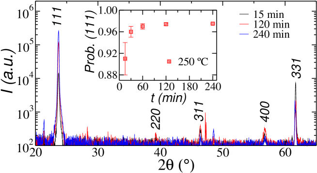
Figure 5.2: X-Ray spectra of CdTe polycrystalline layers using $\lambda_{CuK-\alpha}$. Spectrum for layers grown by (black) 15 min, (red) 120 min, and (blue) 240 min at $T=250\,^{\circ}\mathrm{C}$. One notices the presence of grains with several crystallographic orientations in reference to the substrate normal, namely: (111), (220), (311), (400) and (331). However, as the time evolves, the (111) peak becomes higher. The inset shows the probability of finding a grain whose [111] direction coincides with the normal vector of the substrate surface.

In regard to initial regime of growth, previous studies have shown that the growth of CdTe on H-terminated Si surfaces follows the Volmer-Weber (VW) growth mode, where three-dimensional islands nucleate directly onto the surface without an initial wetting layer [9, 140, 141]. This result has been found in the CdTe growth on both (111) [9, 140] and Si(001) faces [141], by using a slow and/or a variable molecular flux during the experiment. Due to the VW growth mode, conical-like grains are formed onto the template of submonolayer islands and grow by increasing their aspect ratio, since the direct contact with the substrate is unfavorable energetically. Parts of the Si remains exposed until the islands start coalescing to form a continuous layer. As the environment is polycrystalline, grain boundaries (GB) of colided neighborhing grains are unfavorable regions for deposition and diffusion of particles, since in these places one finds a large number of defects [152, 153, 154, 155]. Defects are yielded, mainly, due the stress evolution. Many studies [152, 153] have shown that the stress is compressive prior to coalescence, becomes tensile during the coalescence (as a consequence of attractive forces between neighboring grains) and reaches a constant value as deposition proceeds. Even in the presence of the strong texture, the shared GBs of two (111) crystals also yield defects because the grains have usually different rotational orientations. This kind of defect causes shear stress (torque) which tends to reorient the crystallites [153].

For long growth times (multi-layer regime), the substrate-film interaction is expected to be lost [156] and the growth dynamic becomes dictated by the growth of CdTe on CdTe, i.e. the homoepitaxial growth [156, 157]. As the substrate temperature is high during the growth, the rate diffusion is expected to be high [23]. Thus, “defect sites” at (an around) the GBs of colided neighboring grains are eventually covered by diffusion and deposition of particles (a kind of relaxation process occuring at, and around, these regions), which allows coalescence processes becoming more operative. As consequence of this relaxation, the aspect ratio ($\Omega$) of grains decrease in time and the top of them becomes smoother (due to the “filling” process of particles at local minima), as corroborated by the AFM images (figures 5.1(a)-(e)).

5.2   Local Fluctuations: Non-Universal and Universal Scaling Exponents

Now we turn our attention to local fluctuations at the interface. Figure 5.3(a) shows the local roughness (defined in the section 2.2) calculated for surfaces grown by different times.

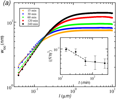
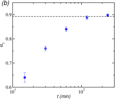
Figure 5.3: (a) Local roughness scaling for CdTe thin films grown at $T=250\,^{\circ}\mathrm{C}$ by 15 min (left triangles), 30 min (up triangles), 60 min (diamonds), 120 min (squares) and 240 min (circles). Inset shows the average local inclination and (b) shows in details the non-universal (geometrical) scaling exponent as function of the growth time. Solid lines in the main plot of (a) represent the fits used to extract $\alpha_{1}$ in (b).

At short length scales ($l\lesssim 10^{-1}$ $\mu m$) and early times, one can observe $w_{loc}(l,t)$ decreasing in time because, in this situation, $w_{loc}$ measures the intra-grain roughness of grains evolving from a sharp to a rounded shape - i.e, from larger to smaller height fluctuations. For comparison, this is the opposite occurring in systems that exhibits anomalous scaling, as can be seen in the appendix section B. In general, the presence or absence of anomalous roughening can be evaluate by calculating the evolution of squared slopes at the surface, $\langle(\nabla h)^{2}\rangle$, which is expected to scale as [70]:

$$\langle(\nabla h)^{2}\rangle\sim t^{2\kappa}.$$ (5.2)

Positive values of $\kappa$ indicate anomalous scaling, while negative or null values confirm that the Family-Vicsek scaling (eq. 2.11) describes the dynamic of local height fluctuations [70, 71].

The inset of the fig. 5.3(a) shows the behavior of $\langle(\nabla h)^{2}\rangle$ in time, which is the same of $w_{loc}$ for fixed box sizes $l^{*}$, with $l^{*}\lesssim 10^{-1}$ $\mu m$. In particular, one can notice that an initial decreasing regime is followed by a “saturated” one. The power-law (eq. 5.2) in this transient regime provides $\kappa=-0.15(5)$. This value is very close to that predicted by López [70], namely $\kappa=-1/6$, for two-dimensional KPZ systems. Moreover, it is well-known that $w_{loc}(l^{*},t)\sim\Omega$ [159, 158] and these results are in agreement with our previous analysis based on AFM images. Moreover, the crossover in $w_{loc}$ occurs in $l\approx\zeta$ (compare with fig. 5.1), in accordance with numerical results [77, 78]. At the other hand, long-wavelength fluctuations ($l\gg 10^{-6}$ $\mu m$) increase in time, as expected [23].

The scaling exponent $\alpha_{1}$, defined as $w(l,t)\sim l^{\alpha_{1}}$, has its value changing in time from 0.6 to 0.9, respectively, as shown in the fig. 5.3(b). These values, however, should not be taken as representative of universal fluctuations at the interface, as done in previous studies [13, 16, 15]. Rather than, as explained by Oliveira and Reis [77, 78] (see section 2.3.2), $\alpha_{1}$ values are related to the grain morphology: $\alpha_{1}\approx 0.6$ indicates that the grainy morphology has a sharp-conical form and, as larger is the $\alpha_{1}$ value, smoother is the top of typical grains’ shape. Notice that these findings are in agreement with the AFM images (fig. 5.1). The true universal roughness exponent $\alpha$, however, should be found in a region where $\zeta\ll l\ll\xi$ [77, 78].

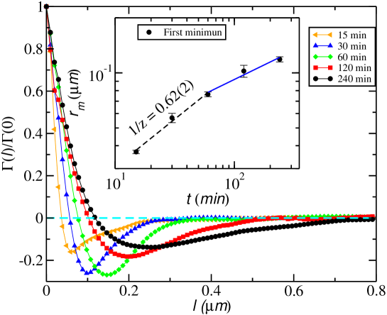
Figure 5.4: Normalized slope-slope correlation function for CdTe thin films grown at $T=250\,^{\circ}\mathrm{C}$ by 15 min (left triangles), 30 min (up triangles), 60 min (diamonds), 120 min (squares) and 240 min (circles). Inset shows the first minimum (circles) extracted from $\Gamma(l)/\Gamma(0)$ curves as function of growth time.

In order to unearth the dynamic exponent, we have used the slope-slope correlation function, defined in the eq. 2.15 and discussed in the section 2.2. Figure 5.4 shows normalized $\Gamma(l)$ functions calculated for all times studied. From the first zero and/or from the first minimum ($r_{m}$) of normalized $\Gamma(l)$ curves one can measure the coarsening exponent $n_{coar}$, defined as $r_{m}\sim t^{n_{coar}}$ [16, 64, 86]. For short growth times, before the appearence of multi-peak structures at surface, one has that $n_{coar}=1/z$. As suggested by AFM images, this regime in our experimental situation occurs for $t\lesssim 60$ min and provide $n_{coar}=1/z=0.62(2)$ - see the dashed line in the inset of the fig. 5.4. This value is in excellent agreement with that expected for two-dimensional KPZ systems [60, 58, 59, 65, 51, 52] (see eq. 3.5). In turn, taking longest available growth times, one obtains $n_{coar}\approx 0.34$, which should not be interpreted as representative of temporal universal fluctuations because, here, peaks of reasonable size appearing on the top of a mound induce an underestimative for the average grain size measured by the slope-slope function (eq. 2.15). Thus, a reliable measurement for $r_{m}$ is not achieved in this situation and, hence, one can not be validated the relation $n_{coar}=1/z$.

5.3   Global Scaling

Following the Family-Vicsek ansätze (eq. 2.11), the global roughness scale as $t^{\beta}$. In the fig. 5.5 one can see the $w$ plot behaving as a power-law with exponent $\beta=0.24(4)$. This is a very strong evidence of KPZ_d=2+1 growth, once $\beta_{KPZ}\approx 0.24$ (see eq. 3.5).

At this point we have found $1/z=0.62(2)$, $\beta=0.24(4)$ and $\kappa=-0.15(5)$. These values are strong indicatives of two-dimensional KPZ growth in CdTe films. If this clue is really true, we should obtain universal distributions of heights, local roughness, and maximal heights matching with that ones numerically predicted for the KPZ class (see table 3.2 and sections 3.2 and 3.3).

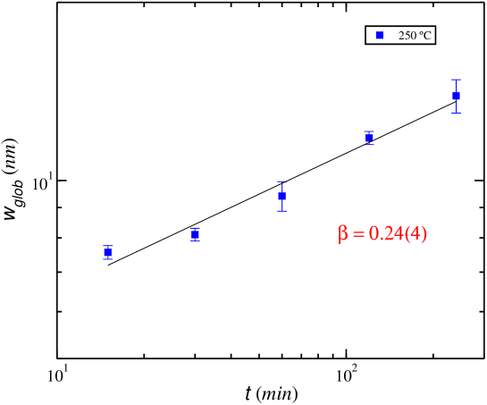
Figure 5.5: Global roughness as function of time for CdTe thin films grown at $T=250\,^{\circ}\mathrm{C}$. The roughness grows as a power-law with $\beta=0.24(4)$.

As we are dealing with a few number of available growth times, we are not able to find the asymptotic velocity ($v_{\infty}$) of the CdTe surface growth [114]. Beyond that, by following the Krug-Meakin toolbox [119, 114], data of CdTe interface fluctuations evolving in time (until reaching the stationary regime) for different initial miscut angles of Si(001) substrates should be accessible. Thus, we are not in position to validate, at this time, the two-dimensional KPZ ansätze (eq. 3.6). However, we can perform a comparison between a rescaled height distributions and the distribution of $\chi$. Take the spatial average on both sides of the eq. 3.4 - negleting the correction terms - one has:

$$\langle h\rangle=v_{\infty}t+sign(\lambda)(\Gamma t)^{\beta}\langle\chi\rangle.$$ (5.3)

One can vanish the term $v_{\infty}t$ subtracting eq. 5.3 from eq. 3.4. The result is:

$$h-\langle h\rangle=sign(\lambda)(\Gamma t)^{\beta}[\chi-\langle\chi\rangle].$$ (5.4)

Now, it easy to show that $\langle h^{2}\rangle_{c}=(\Gamma t)^{2\beta}[\langle\chi^{2}\rangle-\langle\chi\rangle^{2}]$. Hence, dividing eq. 5.4 by the global roughness $w=\sigma_{h}=\langle h^{2}\rangle_{c}^{1/2}$ one finds:

$$\frac{(h-\langle h\rangle)}{\sigma_{h}}=sign(\lambda)\frac{(\chi-\langle\chi\rangle)}{\sigma_{\chi}},$$ (5.5)

where $\sigma_{\chi}$ = $\langle\chi^{2}\rangle_{c}^{1/2}$.

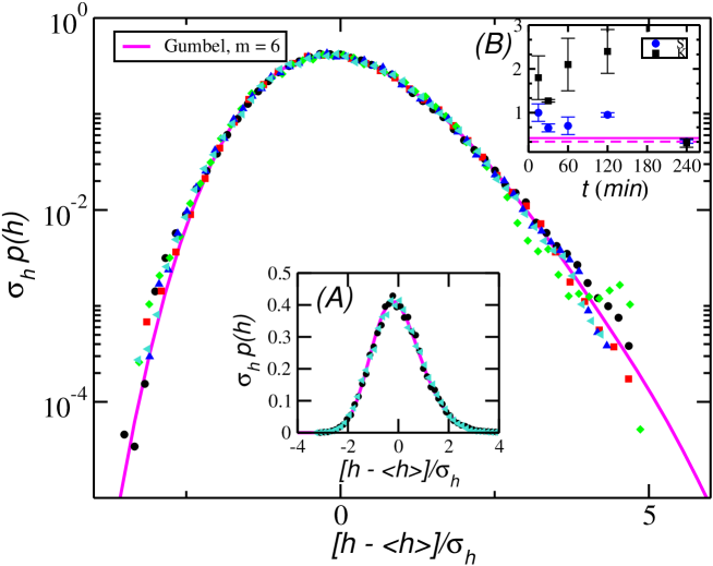
Figure 5.6: Rescaled height distributions at mean null and unitary variance from several regions (symbols) of the thickest sample grown at $T=250\,^{\circ}\mathrm{C}$ compared with the numerical KPZ curve (solid magenta line). Inset (A) highlights the very good collapse between experimental and numerical data close to the peak in a linear $\times$ log plot. Insertion (B) exhibits the experimental S and K evolving in time. Solid and dashed magent lines refers to the numerically expected KPZ_d=2+1 S and K values, respectively.

Equation 5.5 means that to compare rescaled height distributions with mean null and unitary variance is equivalent to comparing the $\chi$ fluctuations rescaled in the same way. This allows us to compare these distributions even without known the non-universal KPZ parameters. Figure 5.6 depicts the rescaled height distributions for several regions of the thickest sample. Remarkably, one notices a very good agreement between the experimental data and the Gumbel pdf with m = 6 (see eq. 3.9) for four decades around the peak. This astonish result is reinforced by the data collapse close to the peak, as highlighted in the the insertion A of the fig. 5.6. The slight deviation observed in the left tail could be due to the fact that AFM tip does not scan accurately deep valleys as well as it does for higher heights.

Comparing the universal KPZ_d=2+1 dimensionless cumulant ratios for the flat case (table 3.2), we have found, for the thickest film, $S_{t=240}=0.34(1)$ and $K_{t=240}=0.3(1)$, while numerical values are $S=0.423(7)$ and $K=0.344(9)$ [60, 58, 59, 65]. However, as shown in the inset B of the fig. 5.6, the experimental $S$ and $K$ values approach to the KPZ_d=2+1 ones only for $t=240$ min. In principle, these results could be just a fluctuation, making the agreement of HDs in the fig. 5.6 a mere coincidence. Indeed, this is not the case here because before to seek the universal HD distribution, critical exponents have already point out to KPZ growth. Moreover, it is well know that experimental $S$ and $K$ values take a long time to converge to the asymptotic values calculated numerically[39, 40, 47]. This effect should be stronger in 2 + 1 dimensional systems. Hence, the underestimate $S$ value can be only a finite-time effect and results emerging from the fig. 5.6 provide the first so-waited experimental confirmation of the KPZ_d=2+1 universality beyond the exponents.

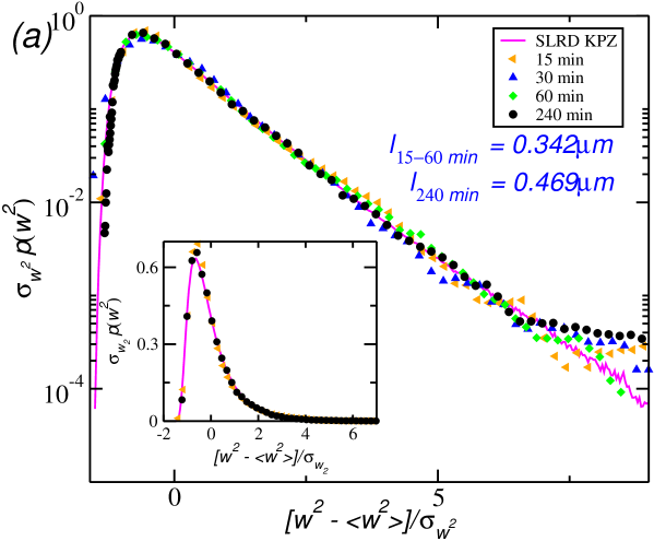
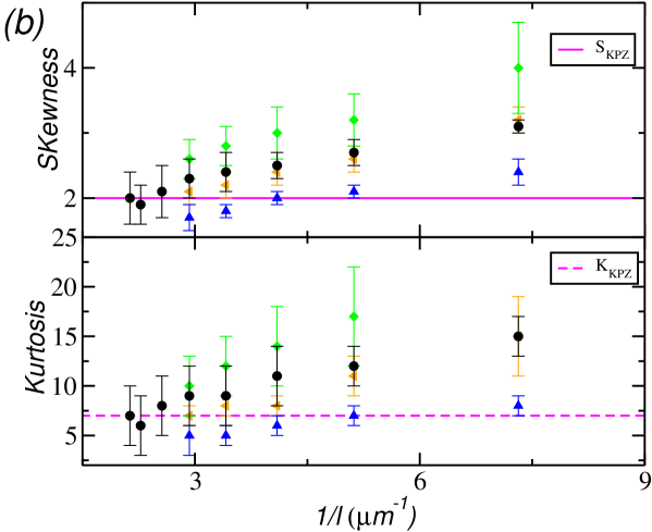
Figure 5.7: (a) Rescaled squared local roughness distributions for samples grown at $T=250\,^{\circ}\mathrm{C}$, by 15 min (orange left triangles), 30 min (blue up triangles), 60 min (green diamonds) and 240 min (black circles).The curves shown are those whose the box size is indicated below the legend. They are different for each $t$ because the appropriate interval $\zeta\ll l\ll\xi$ depends on $t$. The inset shows the good collapse around the peak for the thinnest and thickest film grown. (b) Skewness and kurtosis values as function of the box size $l$.

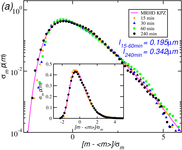
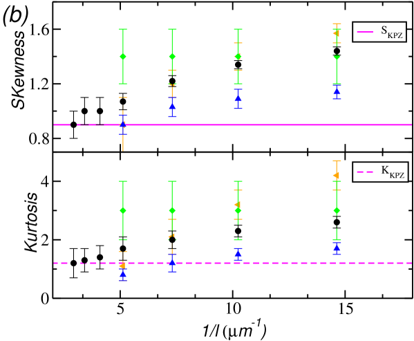
Figure 5.8: (a) Rescaled maximal relative height distributions for samples grown at $T=250\,^{\circ}\mathrm{C}$, by 15 min (orange left triangles), 30 min (blue up triangles), 60 min (green diamonds) and 240 min (black circles). The curves shown are those whose the box size is indicated below the legend. They are different for each $t$ because the appropriate interval $\zeta\ll l\ll\xi$ depends on $t$. The inset shows the good collapse around the peak for the thinnest and thickest film grown. (b) Skewness and kurtosis values as function of the box size $l$.

In order to prove the universality of distributions described in the sections 3.2 and 3.3, and also to gain further evidence of KPZ growth, we have calculated the SLR and MRH distributions, constrained to the box size $l$ within the interval $[10\mu m/1024]\ll l\ll\xi$. Figure 5.7 (a) shows the SLRDs for all available growth times, whereas in fig. 5.7 (b), the respective $S$ and $K$ values as function of $l$ are depicted. Astonishingly, a very good collapse is seen, in almost four decades around the peak, among the experimental and numerical KPZ SRLDs. Moreover, the stretched exponential decay at the right tail is present, giving one more (strong) evidence of KPZ growth.

Similar results are found for the MRHDs, figures 5.8 (a) and (b), where the nice collapse between the experimental and numerical data is evident. The curves showed in the main plot are those whose $S$ and $K$ values better represent the mean for the $l$ described in the graph.

It is very important mention why the $S$ and $K$ values change with $l$. This happens because one does not know, a priori, what are the $l^{\prime}s$ satisfying the condition $\zeta\ll l\ll\xi$ (remember there is a characteristic length at the surface). As in the CdTe/Si(100) system $\zeta\approx\xi$, the appropriate interval for $l$ is very short and should be identified as a convergence of $S$ and $K$ for some specific value. In the case shown in the figures 5.7(b) and 5.8(b), these convergent values agree with those numerically calculated for the SLRD and MRDS of KPZ_d=2+1 models [134, 133, 57].

5.4   The origin of the KPZ mechanism and Conclusions

The results presented in the previous sections point out that the long-wavelength CdTe surface fluctuations, at least for film grown at $T=250\,^{\circ}\mathrm{C}$ and $F\approx 2.2$ Å/s, evolve according to the KPZ equation (eq. 3.1). The origin of the KPZ scaling in this experimental system can be understood unveiling the complex dynamic of grains, which is dictated by an interplay between inter-grain surface energetics, constraints yielded by the coalescence of neighborhing grains and filling processes occuring at (and around) the GB’s of colided neighborhing grains. This leads to a complex packing of crystalline grains. A simple illustration is provided by the grain deposition model in the Ref. [77]. In the model, a new cubic grain is firmly attached to the boundary of the grains below it, but does not fill all available space in their neighborhood because its shape is constrained to be cubic. This aggregation mechanism has the same effect of the lateral aggregation as in the ballistic model [111]. It generates excess velocity, which is the landmark of KPZ scaling.

In conclusion, we have found the first robust experimental $KPZ_{d=2+1}$ system. On the basis of a semi-quantitative morphological and long-wavelength fluctuation studies, we have extracted critical exponents agreeing with that expected for the KPZ class. Moreover, the universality of KPZ distributions (HDs, SLRDs and MRHDs) has been experimentally demonstrated. We have not checked the KPZ_d=2+1 ansätze (eq. 3.4) directly due to inherent two-dimensional experimental obstacles. Our results were published in the Physical Review B [64].

Shortly after the publication of our work [64], T. Halpin-Healy and G. Palasantzas [65] have used this noveil scheme proposed by us to confirm the KPZ universality in oligomer thin films. This clearly corroborates that we have given a new perspective for finding, and confirming, two-dimensional growing surfaces belonging to the KPZ universality class [65].

6   RESULTS: The Effect of Temperature on CdTe Growth Dynamic

In this chapter one studies the effect of the deposition temperature, in the range of [150, 300]$\,{}^{\circ}\mathrm{C}$, on the mound evolution and on the long-wavelength fluctuations of CdTe surfaces grown on Si(001) substrates.

6.1   Intragrain morphology and local fluctuations

Figure 6.1 shows typical AFM images for surfaces grown at different $T$ for the two largest available growth time, $t=120$ min and $240$ min. For $T=150\,^{\circ}\mathrm{C}$ (fig. 6.1(a) and (b)), one can see grains with a well-defined sharp shape dominating the surface, at the same time that $\Omega$ seems to increase with $t$, as suggested by the vertical bar. For films grown at $T=200\,^{\circ}\mathrm{C}$, the scenario is quite similar to that for $T=150\,^{\circ}\mathrm{C}$, except for the largest growth time (fig. 6.1(d)), where $\Omega$ has decreased in the interval of $t\in$ [120, 240]min. Unlike the morphology of surfaces grown at $T=250\,^{\circ}\mathrm{C}$ (fig. 5.1), multi-peaked structures are rare in $t=240$ min and grains with a well-defined shape still are the majority. See fig. 6.2(a), in which typical mound profiles are shown in order to make clear those notes. On the other hand, at higher temperatures, namely $T=300\,^{\circ}\mathrm{C}$, the surfaces present much more complex structures, as can be noticed from the the figures 6.1(e) and (f). In fact, these films are composed by a mix of a few conical grains and large mounds (formed by coalesced grains) with $\zeta\approx 2$ $\mu m$. As the time evolves, $\zeta$ increases faster than the mound height, at least within the interval $t\in$ [120, 240]min, to form larger mounds.

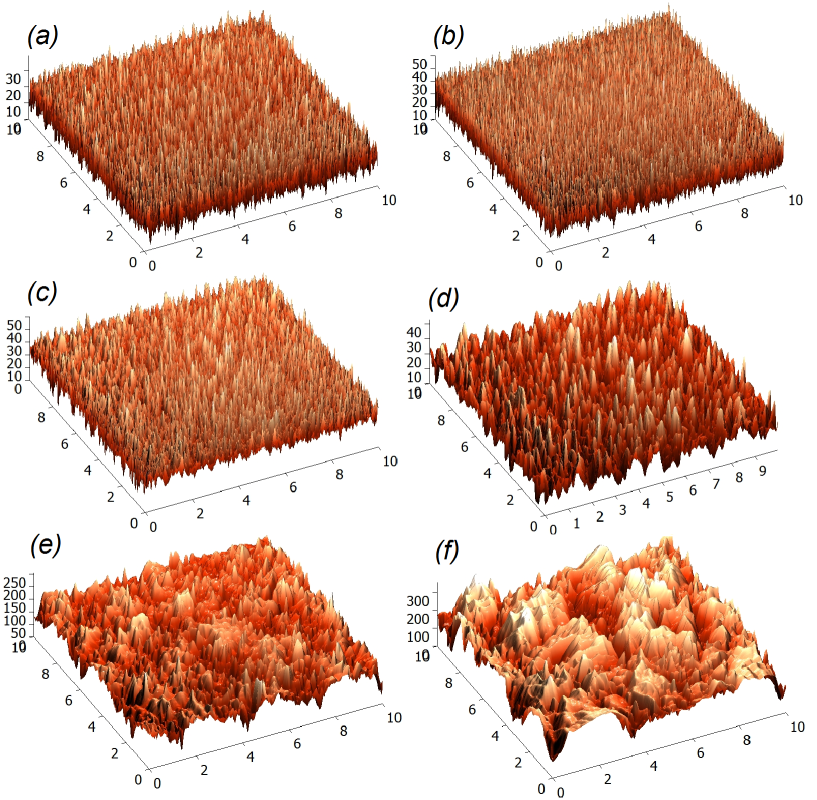
Figure 6.1: AFM images ($10\times 10$ $\mu m$, height scale in $nm$) of CdTe thin films grown at: $T$ = $150\,^{\circ}\mathrm{C}$ (a) and (b), $T$ = $200\,^{\circ}\mathrm{C}$ (c) and (d), and $T$ = $300\,^{\circ}\mathrm{C}$ (e) and (f) by $t=120$ min and $240$ min, respectively.

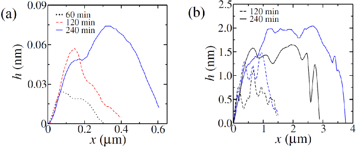
Figure 6.2: Typical grain/mound profiles at the surface for (a) $T=200\,^{\circ}\mathrm{C}$ and (b) $T=300\,^{\circ}\mathrm{C}$ for different growth times.

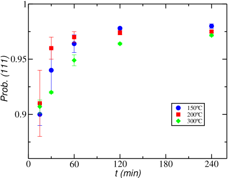
Figure 6.3: Probability of finding (111) grains with respect to the substrate normal in a CdTe layer grown at $T=150\,^{\circ}\mathrm{C}$ (circles), $200\,^{\circ}\mathrm{C}$ (squares) and $300\,^{\circ}\mathrm{C}$ (diamonds).

The orientation of grains whose crystallographic plans are parallel to the substrate surface is determined by $\theta-2\theta$ XRD measurements. As we already found for films grown at $T=250\,^{\circ}\mathrm{C}$, a strong [111] texture has been observed also for other temperatures. Moreover, the same peaks have been seen in the XRD espectra. Figure 6.3 shows the probability of finding (111) grains (eq. 5.1) in the CdTe layer as function of the growth time and for different temperatures. The results suggest that this texture is: 1) slightly influenced by the deposition temperature, being this sligth deviation probably due to the fact that as higher is $T$, larger is the width of grains [160], including those grown in (111)-different orientions which reflects more the X-ray incident and, hence, diminhes $p(111,t,T)$. 2) independent of the substrate, once a similar [111] texture has been found by Ribeiro et al.[14] and Ferreira et. al[9, 142] in the growth of CdTe on glass substrates and also by Sporken et al. using Si(001) substrates [150]. Anyway, the important for the growth dynamic is that most coalescence process happens between (111) grains and, even this way, they give rise a large number of defects at the GBs of colided neighboring grains due to, basically, the difference between the rotational orientation of neighboring crystallites.

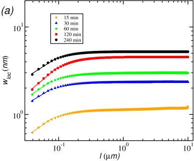
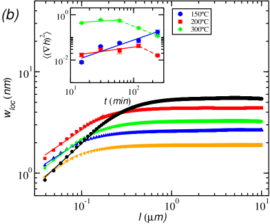
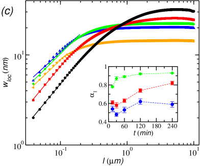
Figure 6.4: Local roughness for films grown at (a) $T=150\,^{\circ}\mathrm{C}$, (b) $200\,^{\circ}\mathrm{C}$ and (c) $300\,^{\circ}\mathrm{C}$ by 15 min (left triangles), 30 min (up triangles), 60 min (diamonds), 120 min (squares) and 240 min (circles). Insertion of (b) shows the squared local inclinations as function of the growth time for $T=150\,^{\circ}\mathrm{C}$ (circles), $T=200\,^{\circ}\mathrm{C}$ (squares), $T=300\,^{\circ}\mathrm{C}$ (diamonds). The same legend is used in the inset of the figure (c), which depicts the geometrical $\alpha_{1}$ exponent as function of $t$, extracted from the solid lines shown in the main plots.

In regard to surface fluctuations at local scales, fig. 6.4 presents the local roughness calculated as function of $t$ and $T$. The first note to take look at is that, in the fig. 6.4(a), the curves dislocate to up as the time evolves (in both short-, $l\lesssim 10^{-1}$ $\mu m$, and large-wavelengths $l\gg 10^{-1}$ $\mu m$) and, apparently, no one relaxation is observed. Indeed, this $w_{loc}$ increasing at short-length scales is the landmark of the anomalous roughening, discussed in the appendix section B, where, at first sight, a larger number of critical exponents must to be found for determining the UC. The $\kappa$ exponent, defined in the equations 5.2 and B.9, has been calculated for the films grown at $T=150\,^{\circ}\mathrm{C}$ - see insertion of the fig. 6.4(b). The value obtained is $\kappa=0.5(1)$. Although this value is positive, indicating anomalous scaling, its particular value is consistent with that one obtained from an uncorrelated interface, where the squared-local-slope fluctuations increase in time with unit power. In another words, the random growth is intrinsically anomalous in this sense.

For surfaces grown at $T=200\,^{\circ}\mathrm{C}$, the situation is more complex than that for the lowest $T$, as shown in the fig. 6.4(b). There, one can see that the curve for $t=240$ min has dislocated down at short-length scales, instead of dislocating up, as in the initial trend. Very interesting, this has been the same behavior presented by $\Omega$, as well as in the visual inspection of AFM images (fig. 6.1). The squared local slopes also show a behavior of two regimes (see inset of the fig. 6.4(b)), where an initial anomalous regime, characterized by $\kappa=0.19(5)$, is followed by a second one in which the Family-Vicsek scaling is asymptotically recovered [83, 70] with $\kappa\approx-0.7$.

For the deposition temperature $T=300\,^{\circ}\mathrm{C}$, the same qualitative result of two regimes is observed - see fig. 6.4(c). The transient anomalous scaling gives place to a “normal” one at $t\lesssim 60$ min, as corroborated by the local roughness at short-length scales and by $\langle(\nabla h)^{2}\rangle$ as function of $t$. The values for $\kappa$ characterizing these two regimes are, respectively, $0.2(2)$ and $-0.56(3)$. Notice that the first value can not guarantee the presence of anomaly, since $\kappa=0$ is a possible value within the error bar.

Now, regarding to the geometrical scaling exponent $\alpha_{1}$, defined as $w_{loc}\sim l^{\alpha_{1}}$ (section 2.3.2), its value as function of the growth time is depicted in the inset of the fig. 6.4(c) for different temperatures. $\alpha_{1}$ is close to $0.6$ for $150\,^{\circ}\mathrm{C}$, which indicates the presence of very sharp grains at surface at all times[77, 78], according with the visual inspection of AFM images. In turn, for $T=200\,^{\circ}\mathrm{C}$ and $300\,^{\circ}\mathrm{C}$, $\alpha_{1}$ changes from $0.6$ to $0.8$ and from 0.80 to 0.95, respectively. This reveals that sharp grains give place to smoother structures at long times. These results are totally consistent with the figures 6.2(a) and (b). A similar behavior for $\alpha_{1}$ occurs for a fixed $t$, as $T$ increases. Based on these results, one can also conclude that the behavior of $w_{loc}$ at short-length scales ($l\ll 10^{-1}$ $\mu m$) is governed by two contributions: the first is the grain shape, related to $\alpha_{1}$, which can present large (sharp grains) or small (flat top grains) fluctuations. The second one coms from the aspect ratio, since for a fized box size $l^{*}$, one has $w_{loc}(l^{*},t)\sim\langle(\nabla h)^{2}\rangle$ [159, 158].

The origin of the results above can be understood as follows: initially, CdTe films evolve according to the Volmer-Weber growth mode [9, 140, 141], and their width becomes larger as higher is the deposition temperature [160] (see fig. 6.1). As the grains with well-defined shape enlarge laterally, they colide forming a continuous film and giving origin to grains boundaries (GBs), where non-crystalline (defects) regions emerge [154, 155]. These GBs fromed by colided neighboring grains are formed mainly at the interface between (111) grains having different rotational orientations. The size of these defect regions is larger as higher is $T$ since large are the grain perimeters (remember that initally $\zeta$ increases with $T$) [160]. At these GBs, hence, an additional energy barrier ($E_{GB}$) rises, which tends to repel the diffusion and the deposition of particles at, and near to, these sites [152, 153]. A similar barrier has also been suggested recently in the growth of CdTe/CdS films [155]. For low $T$, where surface diffusion is slow, a small number of molecules can overcome the $E_{GB}$ barrier and most of them aggregates inside the grain that they have arrived. This compels the grain height to increase faster than its width leading $\Omega$ and $\langle(\nabla h)^{2}\rangle$ to increase as the time evolves (see figs. 6.1, 6.4 and inset of fig. 6.4(b)). However, at long times, a relaxation happens because particles are eventually deposited at (and around) the GBs of colided neighboring grains. This diminishes the number of defect sites in the active zone and, consequently, enhances diffusion towards these regions. From this moment, coalescence processes become more operative and grains with well-defined shape give place to large mounds, so that $\Omega$ and $\langle(\nabla h)^{2}\rangle$ decrease in time. In particular, for $T=150\,^{\circ}\mathrm{C}$ this regime is not observed due to the experimental condition of finite-time growth. For higher $T$, however, the second regime is clearly noticed and appears so earlier as higher is $T$, as can be checked in insets of the figs. 6.4(b) and (c) and in the inset of fig. 5.3(a).

6.1.1   A Kinetic Monte Carlo Model

The reliability of the above reasoning is illustrated in an one-dimensional atomistic growth model. Since our interest is the coalescence process, the growth starts on a periodic array of pyramidal grains with the same width $\zeta$ and height $H$, for simplicity. The unit time is set to correspond to the deposition of one monolayer of particles. During a deposition event, a site i is randomly selected and a particle is allowed diffusing at surface (starting from the site i) until finding a site $j$ where it aggregates permanently whether the constraint $|h_{j}-h_{j\pm 1}|\leq 1$ is satisfied. Thus, inside the characteristic “grain”, aggregation follows the conservative RSOS (restricted solid-on-solid) rule [161]. At the GBs of colided neighboring grains, however, an energy barrier $E_{GB}$ is present, so that a particle diffuses toward them with probability $P_{D}=e^{-E_{GB}/k_{B}T}$. Once a particle aggregates at a given GB $i$, the barrier $E_{GB}$ at $i$ becomes null with probability $P_{R}=e^{-E_{R}/k_{B}T}$. Notice that this simple mechanism captures the underlying feature of the relaxation process at the GBs of colided neighboring grains.

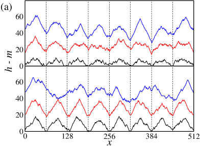
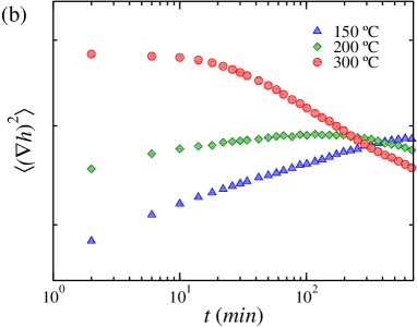
Figure 6.5: Results from an one-dimensional Kinetic Monte Carlo model. In (a) one depicts the height profiles for $T=150\,^{\circ}\mathrm{C}$ (top) and $200\,^{\circ}\mathrm{C}$ (bottom) for $t=10,100$ and 1000, and shifted by $m=10,80$ and 960, respectively. Dashed lines represent the initial (t = 0) GB’s of colided neighboring grains. (b) Average-squared-local slope $\langle(\nabla h)^{2}\rangle$ versus time for surfaces grown at $T=150\,^{\circ}\mathrm{C}$ (circles), $T=200\,^{\circ}\mathrm{C}$ (squares) and $T=300\,^{\circ}\mathrm{C}$ (diamonds).

Figure 6.5(a) shows typical surface evolutions for $T=150$ and $200\,^{\circ}\mathrm{C}$. One has considered $E_{GB}=0.10$ eV, $E_{R}=0.30$ eV, $\zeta=64$ and $H=8$, 16 and 24 for $T=150$, 200 and $300\,^{\circ}\mathrm{C}$, respectively. For $T=150\,^{\circ}\mathrm{C}$ one observes grains with almost fixed width and increasing height. A similar behavior is observed at short times for $T=200\,^{\circ}\mathrm{C}$ but, for large $t$, large mounds (formed by coalesced grains) appears. The same occurs for larger $T$. This qualitative agreement with the experiment is corroborated by the evolution of the squared local slopes displayed in the fig. 6.5(b). Comparing these results with the experimental ones (inset of fig. 6.4(c)), one can confirm that the interplay between the relaxation process at the GBs and initial conditions (Volmer-Weber growth mode and width larger for higher $T$), in fact, explains the CdTe/Si(001) mound evolution. Nevertheless, it is important mention that this simple model does not reproduce (and do not have this intention) the complex dynamic taking place in the growth of CdTe films, but it gives valuable insights about underlying features which rule the coalescence process.

6.2   Universal exponents

Now, once we have got an explanation for what is going on at local scales when the deposition temperature is changed, we are prepared to turn our attention to the analysis of long-wavelength fluctuations and to the Universality Class (UC) of the growth.

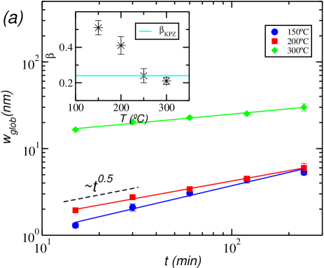
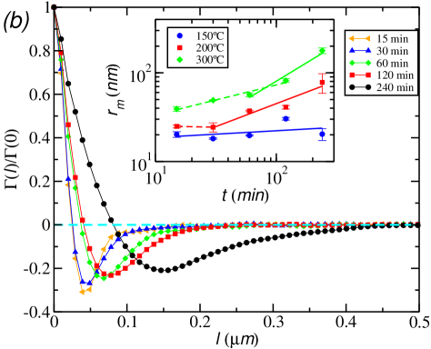
Figure 6.6: (a) Global roughness as function of the growth time for different temperatures, namely, $T=150\,^{\circ}\mathrm{C}$ (circles), $T=200\,^{\circ}\mathrm{C}$ (squares) and $T=300\,^{\circ}\mathrm{C}$ (diamonds). Solid lines are guide to eyes, from which the $\beta$ exponent has been found. Inset of (a) shows how the growth exponent depends on $T$. The solid line marks the value 0.239, which is consistent with $KPZ_{d=2+1}$ [52, 58, 59]. (b) Slope-Slope correlation function for CdTe thin films grown at $T=200\,^{\circ}\mathrm{C}$. The oscillatory behavior is observed for all temperatures and the curve shown is a typical one, valid for all temperatures analyzed. Insertion in (b) depicts the first zero ($r_{m}$) of the Slope-Slope correlation function as a function of time for several $T^{\prime}s$. The legend is the same exhibited in the inset of (a). Dashed and solid lines are guide to the eyes, from where the $n_{coar}$ and $1/z$ exponents have been determined, explained in the text.

Figure 6.6(a) shows the global roughness as function of the growth time for different temperatures. At first, one notices that $w(T)$ increases with $T$. In fact, as the CdTe layer is polycrystalline, the complex competition between grains gives rise to inter-grain fluctuations that are larger as higher is the temperature because: 1) the grains, themselves, are larger and 2) the valleys separating these structures are deeper as higher is $T$, as observed in the fig. 6.1. Similar results have been found in the growth of CdTe grown on glass substrates covered by fluorine doped with tin oxide [16, 13].

Regarding to the growth exponent, for $T=150\,^{\circ}\mathrm{C}$, one obtains $\beta=0.51(4)$ (see inset of fig. 6.6(a)), which in association with $\kappa=0.5(1)$ give us a strong evidence that one has a Poissonian growth at this low temperature. For $T=200\,^{\circ}\mathrm{C}$, however, one can notice that for initial times ($t\lesssim 60$ min), global roughness increases with $\beta_{initial}\approx 0.5$, but this regime is followed by a distinct one where, clearly, one finds a tendency of $\beta$ becoming smaller - compare w(T) for $\textrm{T = 150}\,^{\circ}\mathrm{C}$ and $\textrm{200}\,^{\circ}\mathrm{C}$. Despite this fact, one finds $\beta=0.41(5)$ for $T=200\,^{\circ}\mathrm{C}$. It is worth mention that this value does not match with anyone known UC [23, 26]. In particular this value has been found in homoepitaxial growth of Cu(001) at 250K [162], of Ag(111) and Ag(001) at 300 K [163], and also in the growth of CdTe on glass substrates by HWE at $T=250\,^{\circ}\mathrm{C}$ [13, 16].

Finally, for films grown at $T=300\,^{\circ}\mathrm{C}$, experimental results point out $\beta=0.21(5)$, a value close to the KPZ one (eq. 3.5) [52, 58, 59] and also to the MH and VLDS classes - see section 2.3.1 and appendix section A.3, respectively. Indeed, diffusion should dominate the growth at very higher $T$, overcoming other mechanisms. However, with only this evidence we can not determine which growth equation describes the surface fluctuations of the CdTe interface.

Figure 6.6(b) shows the slope-slope correlation function (eq. 2.15) for CdTe thin films grown at $T=200\,^{\circ}\mathrm{C}$. The same oscillatory behavior is found for samples grown at $T=150\,^{\circ}\mathrm{C}$ and $300\,^{\circ}\mathrm{C}$ (not shown here). As discussed in the section 2.2, from the first minimum or from first zero of $\Gamma(l,t)$, one can extract the average mound size ($r_{m}$), which scales as $r_{m}\sim t^{n_{coar}}$ [16, 64, 86, 18]. In an appropriate range of time, one has $n_{coar}=1/z$. The insertion in the fig. 6.6(b) shows the first zero ($r_{m}$) as function of the growth time, for different temperatures. For $T=150\,^{\circ}\mathrm{C}$, multi-peaked structures do not appear at the surface and the equality $n_{coar}=1/z$ must be valid for all $t$. One finds $1/z\approx 0.07$, which gives one more prove that the growth is uncorrelated at this $T$ [23]. For $T=200\,^{\circ}\mathrm{C}$, two regimes can be reasonably seen, they are indentified as dashed and solid lines in the inset of fig. 6.6(b). From the first regime, one has $1/z\approx-0.02$ and from the second one obtains $1/z=0.6(1)$. The first value is consistent with random growth [23], whilst the second one agree with $KPZ_{d=2+1}$ within the error bar (eq. 3.5) [52, 58, 59]. Finally, for $T=300\,^{\circ}\mathrm{C}$, two short and long-time regimes are also observed and provide $n_{coar}=0.32(5)$ and $n_{coar}=0.7(1)$, respectively. The first regime is consistent with the 1/z value for the VLDS class [23] and the second is near of the expected 1/z value for the KPZ class. Both values agree with numerical ones whithin the error bar. Nevertheless, at this temperature we must be careful in assume $n_{coar}=1/z$, once multi-peaked structures appear since initial growth times. For times $t\lesssim 60$ min, local peaks on the top of the mounds should contribute to underestimate the average size of the structure. However, at large growth times, local peaks become shorter compared with the basis of very large mounds at the surface (see fig. 6.2(b)) and, hence, they should not strongly influence in the measurement of $r_{m}$. Thus, the most careful action should be set $n_{coar}=1/z$ only for long growth times, at least for films grown at high deposition temperatures, as $T=300\,^{\circ}\mathrm{C}$.

6.3   Partial considerations

At this point, we have performed a scaling analysis of CdTe surface fluctuations based also in local features of the growth. From local roughness curves we detect transient anomalous scaling and crossover effects during the dynamic, which have been related to the emergence of an energy barrier at the GB’s of colided neighboring grains and to the relaxation process. A Kinetic Monte Carlo model has supported our reasonings, reproducing qualitatively the experimental results. From the local roughness curves it was not possible to unearth the $\alpha$ exponent because the second (universal) regime has not been observed. However, the values found for $\alpha_{1}$ are consistent with the predictions in the refs. [77, 78] as corroborated by the AFM images - see table 6.1. In the sequence, one has found $\beta$ and $1/z$ as function of the deposition temperature. For $T=150\,^{\circ}\mathrm{C}$, all results indicate a Poisson growth, while for $T=200\,^{\circ}\mathrm{C}$ a crossover from uncorrelated-to-KPZ growth seems to occur. The value $\beta=0.41(5)$, which does not match with any known UC reinforces this idea. For the highest temperature studied, one has $\beta=0.21(5)$ and $1/z=0.7(1)$. The $\beta$ value is close to the MH, VLDS and KPZ classes [23] and prevents a clear distinction of which growth equation describes the CdTe surface fluctuations at this temperature. However, the value found for $1/z$ at long growth times points to a KPZ growth, even at this very high deposition temperature. Moreover, we stress that based only on results coming from exponents, one can not make clear what UC the fluctuations of CdTe surfaces (at T = $200\,^{\circ}\mathrm{C}$ and $300\,^{\circ}\mathrm{C}$) belong.

The values of all exponents found until here can be seen in the tables 6.1, 6.2 and 6.3.

t (min)	15	30	60	120	240
$\alpha_{1}(T=150\,^{\circ}\mathrm{C})$	0.54(3)	0.48(2)	0.53(3)	0.62(3)	0.59(3)
$\alpha_{1}(T=200\,^{\circ}\mathrm{C})$	0.61(2)	0.58(3)	0.63(2)	0.74(2)	0.82(2)
$\alpha_{1}(T=250\,^{\circ}\mathrm{C})$	0.64(2)	0.76(1)	0.84(1)	0.89(1)	0.90(1)
$\alpha_{1}(T=300\,^{\circ}\mathrm{C})$	0.78(1)	0.87(2)	0.89(2)	0.92(1)	0.93(4)

Table 6.1: Values for the non-universal exponent $\alpha_{1}(t,T)$ coming from CdTe surfaces grown on Si(001) substrates by HWE with $F\approx 2.2$ Å/s and deposition temperatures at $150\,^{\circ}\mathrm{C}$, $200\,^{\circ}\mathrm{C}$, $250\,^{\circ}\mathrm{C}$ and $300\,^{\circ}\mathrm{C}$.

$T(\,^{\circ}\mathrm{C})$	150	200	250	300
$\kappa$	0.5(1)	0.19(5)/ $\approx-0.7$	-0.15(5)/ $\approx-0.05$	0.2(2)/-0.56(3)
$n_{coar}$	$\approx 0.07$	-0.02(5)/0.6(1)	0.62(2)/0.35(5)	0.32(5)/0.7(1)

Table 6.2: Values for the non-universal exponents $\kappa(t,T)$ and $n_{coar}(t,T)$ coming from CdTe surfaces grown on Si(001) substrates by HWE with $F\approx 2.2$ Å/s and deposition temperatures at $150\,^{\circ}\mathrm{C}$, $200\,^{\circ}\mathrm{C}$, $250\,^{\circ}\mathrm{C}$ and $300\,^{\circ}\mathrm{C}$. Values separated by the symbol ($/$) are valid in a appropriate range of time. These ranges of time are indicated as solid/dashed lines in the insertion of fig. 6.4(b) for $T=150$, 200 and $300\,^{\circ}\mathrm{C}$ and as dashed/solid lines in the inset of fig. 5.3(a) for $T=250\,^{\circ}\mathrm{C}$.

$T(\,^{\circ}\mathrm{C})$	150	200	250	300
$\beta$	0.51(4)	0.41(5)	0.24(4)	0.21(5)
$1/z$	$\approx 0.07$	0.6(1)	0.62(2)	$0.7(1)$

Table 6.3: Values for the universal exponents $\beta(T)$ and $1/z(T)$ for surface fluctuations of CdTe grown on Si(001) substrates by HWE with $F\approx 2.2$ Å/s within the range of $15$ to $240$ min and for several deposition temperatures.

6.4   Universal Distributions

In this section, we supplement our previous studies with a deep analysis of height, squared roughness local and maximal relative height distribuitons. As we shall demonstrate, this analysis, rather than a complementary one is, in some cases, essential for unveiling the Universality Class of a given growth.

6.4.1   CdTe surface fluctuations at $T=150\,^{\circ}\mathrm{C}$: Poissonian Growth

Figure 6.7 shows the rescaled height distributions for different growth times for CdTe surfaces grown at $T=150\,^{\circ}\mathrm{C}$. The HDs are compared to the Gaussian distribution, expected for uncorrelated growing surfaces. One notices that experimental data collapse very well with the HD-Gaussian near of the peak (inset (A) of the fig. 6.7) as well as at the tails - in at least four decades around the peak.

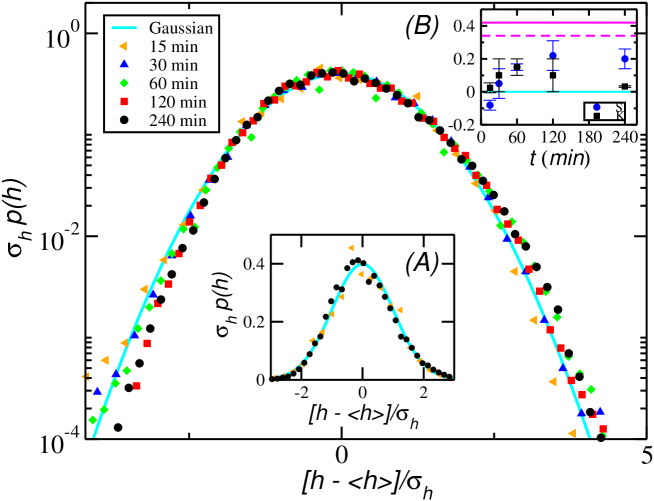
Figure 6.7: Rescaled height distributions at mean null and unitary variance for different growth times (symbols) from CdTe surfaces grown at $T=150\,^{\circ}\mathrm{C}$. The experimental data are compared to the Gaussian (solid cyan line). Inset (A) highlights the very good collapse between experimental data and the Gaussian close to the peak in a linear $\times$ log plot. Insertion (B) exhibits the experimental S and K evolving in time. Solid/dashed cyan and magent lines refers to the S/K values for the Gaussian-HD and KPZ-HD, respectively.

Experimental values for the Skewness ($S$) and Kurtosis ($K$) are displayed in the insertion (B) of the fig. 6.7, where their values seem to fluctuate around zero, as expected from interfaces having a Gaussian-HD. Adding to this result those coming from the scaling roughness analysis (see table 6.3) as well as those from the local dynamic, one can conclude that, at this low temperature, height-field fluctuations of CdTe films are Poissonian [160, 23].

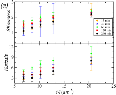
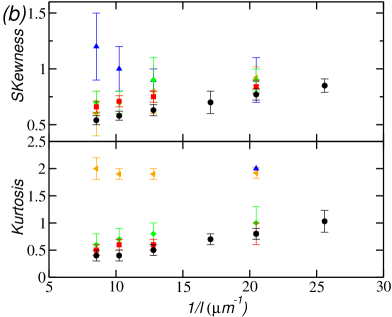
Figure 6.8: $S$ and $K$ values for (a) SLRDs and (b) MRHDs from CdTe surfaces grown at $T=150\,^{\circ}\mathrm{C}$ by 15 min (orange left triangles), 30 min (blue up triangles), 60 min (green diamonds), 120 min (red squares) and 240 min (black circles). No one convergence for S(l) and K(l) curves are observed, as expected for uncorrelated growing surfaces.

The $S$ and $K$ values as function of the box size ($l$) for SLRDs and MRHDs also go in favor to a uncorrelated growth - see figs. 6.8(a) and (b). As discussed in the sections 3.2 and 3.3, these “box” distributions must be evaluated in the range of $\zeta\ll l\ll\xi$. When $l$ satisfies this limit, $S$ and $K$ values become independent of $l$ and converge to universal values [130, 131, 135, 137]. However, when the surface is uncorrelated, $\xi$ keeps very small being of the same order of $\zeta$ (when there are grains at the surface). Thus, no one convergence of $S$ and $K$ should be observed, as can be confirmed in the figures 6.8(a) and 6.8(b).

6.4.2   Random-to-KPZ Crossover in CdTe Surface Fluctuations at $T=200\,^{\circ}\mathrm{C}$

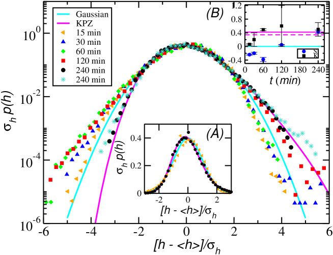
Figure 6.9: Rescaled height distributions, at mean null and unitary variance, for different growth times (symbols) from surfaces grown at $T=200\,^{\circ}\mathrm{C}$. The experimental data are compared to the Gaussian (solid cyan line) and to the numerical KPZ curve (solid magenta line). Inset (A) highlights the very good collapse between experimental and numerical data close to the peak in a linear $\times$ log plot. Insertion (B) exhibits the experimental $S$ and $K$ evolving in time. Solid/dashed cyan lines refers to the Gaussian S/K values, whereas the magenta line indicates the KPZ $S/K$ values.

HDs for CdTe films grown at $T=200\,^{\circ}\mathrm{C}$ can be seen in the fig. 6.9. Very interesting, one notices that the distributions at initial growth times are very far from the KPZ one. Instead, they are closer to a Gaussian. This is confirmed by $S(t)$ and $K(t)$, which are closer to zero than to the KPZ values - see inset B of the fig. 6.9. At long times, however, $S$ and $K$ values seem to converge to the KPZ ones and a very good agreement with the universal KPZ-HD is observed. This disagreement/agreement with a KPZ-HD is reinforced taking into account the collapse near of the peak (see inset A of the fig. 6.9) for surfaces grown at $t=15$ min and $t=240$ min, respectively.

Despite of large error bars related to S and K values, which stem from low statistics, the agreement between the longest growth time available and the expected KPZ values (see table 3.1) is remarkable, namely S${}_{t=240}=0.43(5)$ and K${}_{t=240}=0.5(2)$, whereas KPZ values are $S=0.42(1)$ and $K=0.34(2)$. Based on our previous local and roughening scaling study, we can argue that the HDs above show a crossover in time toward the KPZ regime. In particular, this kind of crossover is widely studied numerically (see [164, 165, 166] and ref. therein) and this experiment, as far as we know, is the first and clean experimental evidence of such random-to-KPZ growth in $d=2+1$.

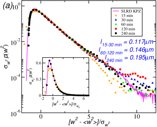
Figure 6.10: (a) Rescaled squared local roughness distributions for samples grown at $T=200\,^{\circ}\mathrm{C}$, by 15 min (orange left triangles), 30 min (blue up triangles), 60 min (green diamonds), 120 min (red squares) and 240 min (black circles). The curves shown are those whose the box size is indicated below the legend. They are different for each $t$ because the appropriate interval $\zeta\ll l\ll\xi$ depends on $t$. The inset shows the poor/nice collapse around the peak for the thinnest/thickest film grown. (b) Skewness and Kurtosis values as function of the box size $l$.

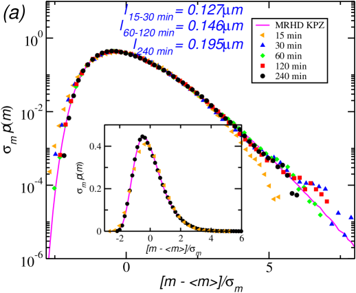
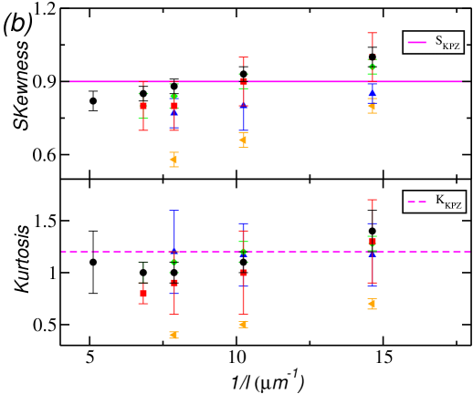
Figure 6.11: (a) Rescaled maximal relative height distributions for samples grown at $T=200\,^{\circ}\mathrm{C}$, by 15 min (orange left triangles), 30 min (blue up triangles), 60 min (green diamonds), 120 min (red squares) and 240 min (black circles). The curves shown are those whose the box size is indicated next to the legend. They are different for each $t$ because the appropriate interval $\zeta\ll l\ll\xi$ depends on $t$. The inset shows the good collapse around the peak for the thinnest and the thickest film grown. (b) Skewness and Kurtosis values as function of the box size $l$.

The SRLDs and MRHDs also support these findings, as exhibited in the figures 6.10 and 6.11. At initial times, SLRDs curves do not present the stretched exponential decay at the right tail, which is known to be a KPZ landmark [133]. Moreover, $S$ and $K$ values for these times do not converge to the KPZ one as the box size is increased (see the fig. 6.10(b)). The comparison between the SLRD for surfaces grown at $t=15$ min and the KPZ-SLRD around the peak gives more evidences of such discrepancy - inset of fig. 6.10(a). Nevertheless, the situation is totally different at long times, where the agreement between the experimental data and the theoretical one reaches more than four decades around the peak with $S$ and $K$ values converging to the KPZ values as the continuous limit is approached, constrained to $\zeta\ll l\ll\xi$. Results coming from the MRHDs (fig. 6.11) are not so accurate as those emerging from SRLDs, but they also corroborate that, for CdTe thin-films grown at $T=200\,^{\circ}\mathrm{C}$, a Random-to-KPZ crossover takes place.

6.4.3   KPZ Growth with Deposition Refused: CdTe Surface Fluctuations at $T=300\,^{\circ}\mathrm{C}$

Finally, the analysis of films grown at $T=300\,^{\circ}\mathrm{C}$ enclose this section and bring to out the real UC of CdTe thin films grown at high temperatures. Figure 6.12 depicts the experimental HDs being compared to numerical KPZ, MH (linear-MBE equation) and VLDS (non-linear MBE equation) curves.

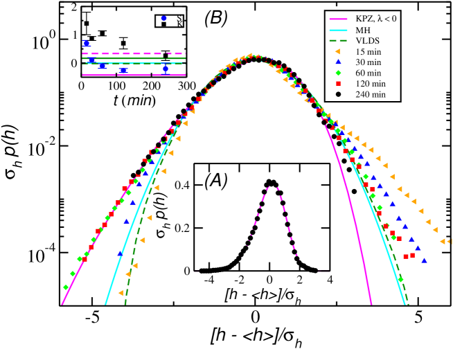
Figure 6.12: Rescaled height distributions at mean null and unitary variance for different growth times (symbols) from surfaces grown at $T=300\,^{\circ}\mathrm{C}$. The experimental data are compared to the numerical KPZ curve (solid magenta line) considering $\lambda<0$, to the universal HD-MH (solid cyan line) and to the universal HD-VLDS (dashed green line). Inset (A) highlights the very good collapse between experimental and KPZ numerical data close to the peak in a linear $\times$ log plot. Insertion (B) exhibits the experimental S and K evolving in time. Solid/dashed lines refers to the expected S/K values.

Just to mention, we have checked the universality for the HDs of these diffusion-dominated classes by integrating the linear equation as well as simulating several discrete models (see [95, 97, 167] and ref. therein) that belong to the MH and VLDS classes. As an additional note, the KPZ HD plotted is that one for $\lambda<0$, which is the same HD plotted in the previous figures, but reflected around the origin. Anyway, one can observe that HDs for early growth times do not agree with distributions of any class, but, for long times, once again, a reasonable agreement with the KPZ-HD is observed. The left tails seem to converge faster than the right ones to the KPZ curve - see HDs for $t>30$ min. As demonstrated by the AFM images (fig. 6.1(e) and (f)) and by the local exponent $\alpha_{1}$ (inset of the fig. 6.4(c)), the top of grains become smoother as the time evolves. It leads the right tail of the HDs to move in the left direction and, consequently, to approach to the KPZ-HD.

Unlike the exponents, the experimental HDs discard the MH and VLDS classes as possibles UC of the CdTe growth. For the largest time available, the inset A of the fig. 6.12 presents a nice collapse around the peak between the experimental result and the numerical one. Moreover, it is clear seen that $S(t)$ and $K(t)$ values are approaching to the KPZ ones, within the error bars - inset B of the fig. 6.12. Particularly, for $t=240$ min, one has S${}_{t=240}=-0.2(2)$ and K${}_{t=240}=0.3(2)$, which agree with the KPZ values (table 3.1), for $\lambda<0$, considering the large error bars.

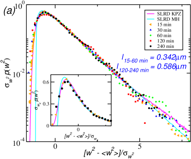
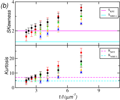
Figure 6.13: (a) Rescaled squared local roughness distributions for samples grown at $T=300\,^{\circ}\mathrm{C}$ by 15 min (orange left triangles), 30 min (blue up triangles), 60 min (green diamonds), 120 min (red squares) and 240 min (black circles). The curves shown are those whose the box size is indicated below the legend. They are different for each $t$ because the appropriate interval $\zeta\ll l\ll\xi$ depends on $t$. The inset shows the good collapse around the peak for the thinnest and the thickest film grown. (b) Skewness and Kurtosis values as function of the box size $l$.

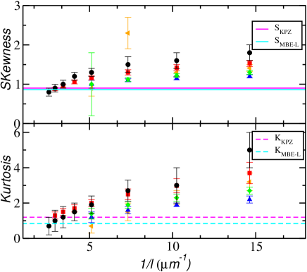
Figure 6.14: $S$ and $K$ as function of the box size for MRHDs for samples grown at $T=300\,^{\circ}\mathrm{C}$. Solid/dashed line indicates the expected values for the $S$ and $K$ for the KPZ (magenta line) and for the MH class (cyan line).

To gain further evidence of KPZ scaling, the SLRDs and MRHDs have been calculated and are depicted in the figures 6.13 and 6.14, respectively. From the left tail and from the peak of the SLRDs (fig. 6.13 and its inset), one notices that experimental results are very well described by the KPZ curve, whereas the decay at the right tail can not make a clear distinction between the KPZ and the MH class. In the fig. 6.13(b), $S$ values converge to the KPZ ones, in the meantime that $K$ values also can not be distinguished from that expected for the KPZ-MRHD and MH-MRHD. In this situation, where the exponent analysis point to KPZ or to MH growth, the MRHDs are not suitable to make a separation between these two classes. As showed in the fig. 6.14, the expected $S$ and $K$ values for the KPZ and the MH class are very close between each other and, from the experimental point of view, one can not distill the UC based only on this result.

These findings help us to see how hard is determining the UC of the two-dimensional experimental films. Anyhow, guided by the local-structure evolution, roughening scaling results $\&$ distributions analysis, we can conclude that the CdTe interface for $T=300\,^{\circ}\mathrm{C}$ evolves according the KPZ equation (eq. 3.1) with $\lambda<0$. This indicate the existence of a mechanism of refusing the deposition of particles depending on the local slopes as occurs in the famous RSOS model [129]. A possible explanation for $\lambda<0$ is that the sticking coefficient is smaller in regions with very large slopes at surface. Indeed, one notices in the fig. 6.4(b) that $\left\langle(\nabla h)^{2}\right\rangle$ for $T=300\,^{\circ}\mathrm{C}$ is very larger than that for lower $T$. This can explain why this effect appears only at high $T$ [62, 168].

6.5   Final Remarks

A detailed study on how the deposition temperature affects the CdTe growth dynamic in a wide range of temperature [150, 300]$\,{}^{\circ}\mathrm{C}$ has been performed. The local mound evolution has been explained in terms of an interplay between a local energy barrier $E_{GB}$ that tends repelling the diffusion and the deposition of particles at defect sites (yielded by the colision of GBs of neighboring grains) and the effectiveness of the relaxation process at these GBs, which tends to eliminate defects on the active zone of the CdTe interface. In turn, the last mechanism depends sensintively on the substrate temperature. Thus, for $T=150\,^{\circ}\mathrm{C}$, the low diffusion at the GBs of colided neighboring grains prevents coalescences and the propagation of correlations at interface, so that inter-grain fluctuations are described by Possianian process. This dynamic also happens at short times for films grown at $T=200\,^{\circ}\mathrm{C}$, however the relaxation at (and around) the GB’s of colided neighboring grains gives rise to coalescences and, hence, an asymptotic correlated growth. For higher $T$, where diffusion rate is higher, these processes start early as well as the KPZ scaling.

In terms of KPZ equation (eq. 3.1), the random growth at low $T$ implies $\nu\approx 0$ and $\lambda\approx 0$. For $T=200\,^{\circ}\mathrm{C}$, one expects $\lambda>0$, but small, so that growth is dominated by noise/non-linear effects initially/asymptotically. The absence of a crossover when $T=250\,^{\circ}\mathrm{C}$ [64] indicates that $\lambda$ is positively large. The same interplay also takes place in this temperature, but as the diffusion is still more operative than that for lower $T$, coalecence processes start early enhancing the activity the grain-packing (discussed in the previous chapter) and, hence, the strength of $\lambda>0$. Thus, $\lambda(T)$ seems to be a positive increasing function in this range of $T$. However, for $T=300\,^{\circ}\mathrm{C}$, the evidences of KPZ scaling and the negative skewed HDs-KPZ reveals $\lambda<0$, which is typical of KPZ systems where there is deposition refuse as in the RSOS model [129]. A possible explanation is that the the sticking coefficient becomes smaller in regions with very large slopes at surface. This reasoning is corroborated by $\left\langle(\nabla h)^{2}\right\rangle$ for films grown $T=300\,^{\circ}\mathrm{C}$, where one confirms the presence of larger slopes than those for lower $T$. This can explain why this effect appears only at high $T$ [62, 168]. Anyway, it is astonishing that so contrasting KPZ mechanisms can emerge in the CdTe growth system only adjusting $T$.

7   Conclusions and Perspectives

In this work one has performed a detailed study on the growth dynamic at both short- and large-wavelength scales of CdTe thin films grown on Si(001) substrates by Hot Wall Technique. The results have provided, for the first time, a clear and robust evidence of a system in d = 2 + 1 dimensions which belongs to the Kardar-Parisi-Zhang class. Here, the phrase “robust evidence” means that the prove goes beyond the comparison with critical exponents, as confirmed by the (rescaled) height distributions, squared local roughness distributions and maximal relative height distributions. In the meantime, this work demonstrates the universality of these KPZ distributions, giving them a reliable reality beyond numerical simulations.

Along the analysis, one has found several pitfalls hampering the extraction of asymptotic scaling exponents. For instance, through the power-law in the $w_{loc}\times$ l plot, it was not possible to unearth the roughness exponent. Rather than, only the geometrical exponent, $\alpha_{1}$, which does not provide any information about the Universality Class (UC) of the system, was found. Another difficulty is the relation between the average mound size ($\zeta$) and the correlation length ($\xi$). The validity of $\zeta\approx\xi$ should be taken as true only for an appropriate range of time, for which local peaks on the top of large mounds do not strongly underestimate the measurement of $\zeta$. Thus, an initial deep-visual inspection of surfaces imaged by some microscope technique becomes important.

The KPZ mechanism occurring in CdTe films grown at $T=250\,^{\circ}\mathrm{C}$ is related to the form in which new particles attaches to grain boundaries (GBs) of colided neighboring grains, do not filling all available space in their neighborhood and, thus, generating excess of velocity, the KPZ landmark. As will be discussed below in details, this packing mechanism also should be present in other temperatures. Due to inexorable experimental obstacles it was not possible to validate the KPZ Ansätze in d = 2 + 1 dimensions. However, this is a natural extension of this work.

The effect of the deposition temperature ($T$) on the growth dynamic has also been distilled in broad range of $T$, namely, $T\in$ [150, 300]$\,{}^{\circ}\mathrm{C}$. A relation between short- and large-wavelength dynamics has been established. One has been found that the mound evolution is dictated by the interplay between the formation of defects at grain boundaries of colided neighboring grains and the relaxation process induced by diffusion and deposition of particles toward these regions. A simple Monte Carlo model corroborate this reasoning. This interplay leads to different scenarios at large-wavelength fluctuations as $T$ increases. For $T=150\,^{\circ}\mathrm{C}$, the low diffusion at the GBs prevents coalescences and the propagation of correlations at interface, so that inter-grain fluctuations are described by a Poissonian process. Scaling exponents and distributions give support to these reasonings.

For $T=200\,^{\circ}\mathrm{C}$, however, a more complex scenario has been found. In the range of growth time studied, the relaxation process overcomes the effects of the barrier at (and around of) the GBs and gives rise to a crossover in the CdTe growth dynamic. Results from dynamical scaling and distributions also corroborate with the presence of this crossover. Roughness scaling analysis, nevertheless, have not been able to, convincingly, point the UC of the CdTe growth at this deposition temperature. The supplemental study based on the distributions, in turn, have proved itself be essential for unveiling the UC of this system, once weaker finite-time effects than that in the standard roughness scaling has been found. Thus, it was possible to find a Random-to-KPZ crossover taking place in the CdTe growth, at the same time that the first robust experimental realization of such crossover in two-dimensional systems is demonstrated.

The growth of CdTe films at $T=300\,^{\circ}\mathrm{C}$ carries also its distinct importance. Although dynamical scaling analysis do not allow making a clear distinction among diffusion-dominated equations and the KPZ one for describing CdTe fluctuations at this high deposition temperature, the distributions discard the formers and point out the presence of KPZ growth with $\lambda<0$, differently of lower temperatures. This unanticipated result has been related to the decreasing of the sticking coefficient in regions with very large slopes at surface. The reasoning is corroborated by the squared-local slopes, which are about five times larger than those for lower temperatures, as can be noticed in the Atomic Force Microscope images. This can explain why this KPZ mechanism appears solely at high temperatures.

In terms of the KPZ equation (eq. 3.1), the results reveal that, for $T=150\,^{\circ}\mathrm{C}$, the “surface tension” ($\nu$) and the excess of velocity ($\lambda$) are very near of zero, so that noise dominates the growth. For CdTe films grown at $T=200\,^{\circ}\mathrm{C}$, however, the Random-to-KPZ crossover found indicates $\lambda>0$, but small, so that non-linear effects overcome the noise only at long growth times. In turn, a clean evidence of the KPZ scaling since inital growth times is present in CdTe films grown at $T=250\,^{\circ}\mathrm{C}$, in which $\lambda$ is positive and large. At the moment that all conspire to conjecture $\lambda(T)$ as an increasing function of $T$, the results coming from CdTe films grown at $T=300\,^{\circ}\mathrm{C}$ show that $\lambda$ is negative. This suggests that i) is possible to adjust $T$ at some specific $T_{EW}$, with $T\in$ ]250, 300[$\,{}^{\circ}\mathrm{C}$, in order to obtain $\lambda=0$, i.e, to have a growth described by the Edwards-Wilkinson equation and ii) to set $T_{(EW-KPZ)}=T_{EW}\pm\delta T$, so that EW-to-KPZ crossovers emerge into the dynamic of CdTe surface fluctuations. In summary, it is possible to adjust the KPZ non-linearity in the CdTe system only adjusting the deposition temperature. Figure 7.1 summarizes theses discussions, making clear different regimes that takes place in the growth as T is increased, namely: region I refers to the temperature interval in which a Poissonian(Random)-to-KPZ crossover rules the dynamic. This first region is localized at the rigth border of temperatures close to $150\,^{\circ}\mathrm{C}$, where $\lambda\rightarrow 0$ and where the Poissonian(Random) growth emerges; in the region II a clean KPZ scaling emerges and precedes the thin III regime, limited by $T=T_{EW}\pm\delta T$ and symmetric in relation to the $T_{EW}$ point, in which the pure EW growth ($\delta T=0\,^{\circ}\mathrm{C}$) and the EW-to-KPZ crossover are expected to take place. Finally, at high temperatures (although expected do not be much higher than $300\,^{\circ}\mathrm{C}$), the KPZ scaling is recoreved with $\lambda<0$.

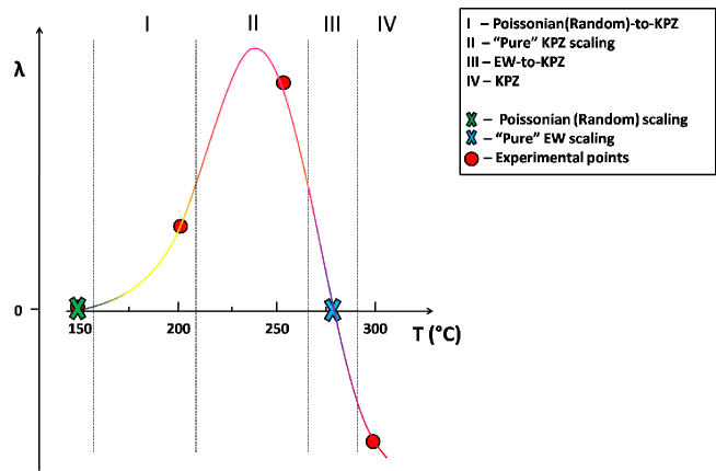
Figure 7.1: Conjecture for the behavior of the excess of velocity, $\lambda$, as function of the deposition temperature $T$ in the CdTe/Si(001) system. Circles refer to experimental points, and dashed lines indicates expected different regimes (I to IV) ruling the coarsening-grained dynamic. The “$\times$” point denotates temperatures for which global fluctuations are expected to belong to Random (green $\times$) and EW (blue $\times$) Classes.

We finish this work truly believing that the noveil procedure for investigating the UC of growing surfaces open and will motivate (as exemplified by T. Halpin-Healy and G. Palasantzas [65]) a new confident perspective in the field, as well as the application of these methods in previously studied systems. Our system also offer the experimental possibility of a close study of Random-to-KPZ and EW-to-KPZ crossovers.

Appendix A More Details About Continuum Growth Equations and Universality Classes

A.1   Random Growth equation

Concerning on EW and linear-MBE equations, one can easily see the particular case, where $\nu$ and $K$ are nulls respectively, resulting in the so called Random Growth equation:

$$\partial_{t}h=\eta(\textbf{x},t).$$ (A.1)

Once just the noise rules the growth dynamics, there are no correlations to be propagated through the system and we can argue $z\rightarrow\infty$. The $\alpha$ exponent is also ill defined, since the system never reaches the stationary regime. Nevertheless, we still can find as the variance of such random interfaces evolves with the deposition time. The result is anticipated if one looks at these surfaces as being composed by a set of independent Brownian motions.

Integrating the random eq. one obtains: $\int\partial_{t}h(\textbf{x},t)dt=\int\eta(\textbf{x},t)dt$. Averaging both sides, one has $\langle h(\textbf{x},t)\rangle=0$. But, if instead we square and average, one reaches $\langle h^{2}(\textbf{x},t)\rangle=2Dt$. So, the variance grows as in the eq. A.2, defining the “growth exponent” $\beta=1/2$.

$$w^{2}(t)=\langle h^{2}\rangle-\langle h\rangle^{2}=2Dt.$$ (A.2)

A.2   A derivation for the Linear-MBE equation

It is well known that in MBE environments, under usual conditions, desorption is a negligible process and, hence, the therm $\nabla^{2}h$ in the eq. 2.19 should not play an important role. Formation of overhangs and bulk defects are uncommon in the ideal epitaxy [156, 157] and discard the non-linear $(\nabla h)^{2}$ term. Our starting point for building a continuum growth equation for MBE environments is the conservation law:

$$\partial_{t}h=-\nabla\cdot\textbf{J}+\eta(\textbf{x},t),$$ (A.3)

where J represents a parallel current of particles diffusing onto the interface.

As interfaces growing in MBE chambers are driven by chemical bond in order to minimize their surface free energy through diffusion, J should be $\propto-\nabla\mu$. But the simplest assumption, in turn, points out that the chemical potential is proportional to $-1/R$, where R is the local curvature - see fig. A.1. The bottom of a valley (positive curvature, $R>0$), for instance, is the site where a particle have major number of neighbors and move away from there will be difficult. So, the bottom of a valley is a minimum for $\mu(\textbf{x},t)$. The opposite happens for the topest site of a island ($R<0$), where there is a local maximum for $\mu(\textbf{x},t)$. On a terrace, all particles have the same coordination number, and locally $\mu=0$ everywhere. Hence, on these considerations one can argue straightforwardly $\mu(\textbf{x},t)\propto-\nabla^{2}h$. Consequently, $\textbf{J}\propto\nabla(\nabla^{2}h)$ and one reaches to the eq. 2.23, after eq. A.3.

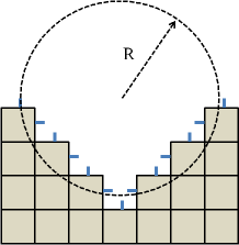
Figure A.1: Schematic of the chemical potential depending on the local curvature. At left to rigth: positive curvature, showing a valley, where there is a local minimum of $\mu(\textbf{x},t)$ because particles sticked at the bottom of the valley will not move away from there. On a terrace $R\rightarrow\infty$ and $\mu(\textbf{x},t)$ is null everywhere. Negative curvature, showing an island, where $\mu(\textbf{x},t)$ has a local maximum value because particles on the top of the island break off their bonds and hop to a closest neighbor site where the free energy of the interface is decreased.

A.3   The Non-Linear MBE equation and the VLDS class

In models with conserved dynamic, there is necessity of inserting non-linear terms, since $\alpha>1$ breaks the hypothesis that continuum approximations are valid in the limit of small slopes, $\nabla h\ll L^{\alpha-1}$ [23]. As pointed out by Wolf and Villain [73], the lowest non-linear term obeying conserved dynamic is the therm $\nabla^{2}(\nabla h)^{2}$. The geometrical interpretation (see ref. [169]) indicates that particles landing at high steps (large derivatives) relax to lower steps (small derivatives), corresponding to the “high-temperature” regime in MBE environments, where atoms break their bond and diffuse, with larger bias, to small slope kinks. The non-linear MBE equation (eq. A.4) was proposed formally in 1991 by Lai and Das Sarma [169].

$$\partial_{t}h(\textbf{x},t)=-K\nabla^{4}h+\lambda_{1}\nabla^{2}(\nabla h)^{2}+\eta(\textbf{x},t),$$ (A.4)

$\lambda_{1}$ has the same dimension of $\nu$ and accounts for the strength of diffusion of particles at local slopes towards small derivatives.

Critical exponents related to the non-linear MBE equation can be found by using Renormalization-Group (RG) approaches [169, 23]. The method predicts:

$$\alpha=\frac{4-d_{s}}{3};\qquad z=\frac{8+d_{s}}{3}$$ (A.5)

Other very important result coming from RG analysis is the hyper-scaling relation valid for any growth with conserved dynamic and non-conversed noise:

$$z-2\alpha-d_{s}=0$$ (A.6)

The set these exponents compose the Villain-Lai-Das-Sarma (VLDS) Universality Class. There are a small number of discrete models belonging to the VLDS class, among which possibly are the conserved restricted-solid-on-solid (CRSOS) model, proposed by Kim et al. [161] and the Das Sarma and Tamborenea one (DT) [92]. A very good numerical study and descriptions of these models can be found in the Ref. [167].

Appendix B Anomalous Scaling

Anomalous scaling occurs whenever a surface is not self-affine [68]. It means that local and global fluctuations do not evolve in the same way. Initially, the therm anomalous was used to describe the growth of interfaces in which the exponent $\alpha$ was found to be larger (or equal) than 1 [170, 171, 67, 172]. Indeed, this comes from the fact that, if $\alpha\geqslant 1$, there is a divergence of fluctuations in the steady state, making the surface super-rough, as indicated by the Family-Vicsek ansätze (eq. 2.11): $W_{sat}/L\sim L^{\alpha-1}$.

The current situation, however, is very different from that of almost twenty years ago. Nowadays, one knows that several systems display anomalous scaling, independently of the $\alpha$ value (see [71, 72] and references therein). Moreover, there are more than one possible scaling form to describe the local-fluctuations dynamic of a growing interface, being the FV one only a particular case where there is no difference between the local and global one [71]. A wide number of experimental studies have also corroborated this conjecture, among which are the development of wood fractures [173], the electrodeposition of Cu [159], the dissolution of pure iron [86] and the deposit of colloidal particles at the edge of evaporated drops [174].

The initial clues of a break in the FV hypothesis were found in the one-dimensional Wolf-Villain model [67, 74] and, subsequently, in other linear and non-linear growth models dominated diffusion [171, 172, 74, 97]. From there, analytical and numerical treatments were strongly devoted to this issue, leading to the conclusions:

• The condition $\alpha<1$ is not sufficient to prevent the system of exhibiting the anomalous scaling [68].

• There exist three types of anomaly: super-rough, intrinsic [69] and faceted [71] (they are defined below).

• Non-conserved growth models do not exhibit anomalous scaling and, in particular, intrinsic scaling can not occur in local growth models [70, 72].

It is worth mention that the presence of the anomaly affects only local correlation functions, keeping the global roughness, for instance, scaling according to the standard FV scaling [71] - this is proved in the following. For now, consider the Fourier transform of the function $h(\textbf{x},t)$ as,

$$\textrm{\^{h}}(\textbf{k},t)=L^{-d_{s}/2}\sum_{\textbf{x}}[h(\textbf{x},t)-\langle h(t)\rangle]\exp({i\textbf{k}\cdot\textbf{x})},$$ (B.1)

where k are the wave-numbers surviving within the space bounded by the substrate.

The called structure factor [$S(k,t)$] or power spectrum (eq. B.2) is a correlation function measuring the fluctuations in the reciprocal space.

$$S(k,t)=\langle\textrm{\^{h}}(\textbf{k},t)\textrm{\^{h}}(\textbf{-k},t)\rangle=\langle|\textrm{\^{h}}(\textbf{k},t)|^{2}\rangle.$$ (B.2)

$S(k,t)$ can be related to the global roughness and to the height-height correlation function ($C_{h}$) by the eqs. B.3 and B.4, respectively,

$$W^{2}(L,t)=\frac{1}{L^{d_{s}}}\sum_{k}S(k,t)=\int\frac{d^{d_{s}}{k}}{(2\pi)^{d_{s}}}S(k,t),$$ (B.3)

$$C_{h}(l,t)\propto\int[1-cos(\textbf{k}\cdot\textbf{x})]\frac{d^{d_{s}}{k}}{(2\pi)^{d_{s}}}S(k,t),$$ (B.4)

where the integrals run within the interval $2\pi/L\leq k\leq 2\pi/a$ for each $k$ direction, with $a$ being the lattice parameter.

The basic tools required to derive the different forms that anomalous scaling can appear are written in order in the equations above. Inserting the FV ansätze (eq. 2.11) into the relation of eq. B.3, it is straightforward showing that the power spectrum behaves as:

$$S(k,t)=k^{-(2\alpha+d_{s})}s_{FV}(kt^{1/z}),$$ (B.5)

where:

$$s_{FV}(u)\sim\left\{\begin{array}[]{c}const,\quad if\quad u\gg 1,\\ u^{2\alpha+d},\quad if\quad u\ll 1.\end{array}\right.$$ (B.6)

It means that for short-length scales ($k\gg 1/\xi$), the power-spectrum is time-independent and the curves for all times show a power-law scaling with $k^{-(2\alpha+d_{s})}$. This is the usual FV scaling in the reciprocal space. But now, look what happens when this scaling relation is inserted into the eq. B.4. When one sets $\alpha>1$, the integral in eq. B.4 becomes divergent in the limit of $l\ll\xi$ for $L\rightarrow\infty$, and $a\rightarrow 0$ [69]. Taking the limit $l\ll\xi$ first, and keeping $L$ and $a$ fixed, one obtains a different scaling relation for $C_{h}$:

$$C_{h}(l,t)\sim\left\{\begin{array}[]{c}l^{2}t^{2(\alpha-1)/z},\quad if\quad l\ll\xi\ll L,\\ l^{2}L^{2(\alpha-1)},\quad if\quad l\ll L\approx\xi.\end{array}\right.$$ (B.7)

So now a different roughness exponent has emerged and, locally, $C_{h}(l,t)\sim l^{2(\alpha_{loc})}$, where $\alpha_{loc}\neq\alpha$ and $\alpha_{loc}=1$. Moreover, a dependence in time for $C_{h}$ at wavelengths $l\ll\xi$ appears in the system scaling with $t^{2\kappa}$, where:

$$\kappa\equiv(\alpha-\alpha_{loc})/z.$$ (B.8)

Translating this scaling for the context of the fig. 2.3, one would see the curves for different growth times, shown in that figure, shifted to up as the time evolves for $l\ll\xi$. Figure B.1(a) shows very clearly this non-usual behavior by calculating the square-local-slope evolution (eq. B.9) for the one-dimensional Wolf-Villain model [67].

$$\langle(\nabla h)^{2}\rangle\sim C_{h}(l=1,t)\sim t^{2\kappa}.$$ (B.9)

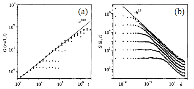
Figure B.1: Example of anomalous scaling. In (a) one has the function G(1,t) (corresponding to the $C_{h}(1,t)$ function) for several systems sizes L (from the bottom o the top L = 10, 15, 30, 60, 120, 240, 800 and 1024, respectively). (b) Shows the non-usual behavior for the structure factor S(k,t). From the bottom to the top the curves refer to growth times t = $2^{4}$, $2^{7}$, $2^{10}$, $2^{13}$, $2^{16}$, $2^{19}$, $2^{22}$, respectively. Figure extracted from ref. [67].

In the WV model, it was found $\kappa=0.19(1)$ during a transient regime, limited by both finite-size and finite-time corrections [67]. But this feature of non-usual behavior of correlations functions at local scales is not the complete scenarium in which the anomaly can emerge. Indeed, models incorporating random diffusion [69] and diffusion-dominated [175] presented a non-usual behavior not only for $C_{h}(l,t)$, but also for the power spectrum, i.e [S($k\gg 1/\xi$,t)] is time dependent - see fig. B.1(b). Thus, it became clear that the FV ansätze written in the reciprocal space (eq. B.6) could not be the general scaling dictating local fluctuations in the surface growth context.

The generic dynamic scaling in kinetic roughening has been developed along of many years [68, 69, 70], but a formal deduction has been achieved in the year of 2000, where Ramasco et al. [71] have proposed a scaling for $s(u)$ as,

$$s(u)\sim\left\{\begin{array}[]{c}u^{2(\alpha-\alpha_{s})},\quad if\quad u\gg 1,\\ u^{2\alpha+d},\qquad if\quad u\ll 1,\end{array}\right.$$ (B.10)

where $\alpha_{s}$ is a new exponent called spectral roughness exponent.

Thus, the power-spectrum, generically, scales as:

$$S(k,t)\sim\left\{\begin{array}[]{c}k^{-(2\alpha_{s}+d_{s})},\quad if\quad k\gg 1/t^{1/z},\\ t^{\frac{2\alpha+d_{s}}{z}},\qquad if\quad k\ll 1/t^{1/z}.\end{array}\right.$$ (B.11)

Inserting eq. B.10 in eq. B.3, one proves that global fluctuations are dictated by the standard Family-Vicsek scaling (eq. 2.11), independently of $\alpha$ and $\alpha_{s}$ values. Nevertheless, as we have shown above, the local scaling is modified, depending on the order of the several limits involved and on values of the exponents [71]. In a general way, two major cases can be distinguished, namely, $\alpha_{s}<1$ and $\alpha_{s}>1$. For the former, one obtains the same that in the eq. 2.10, but with $L\rightarrow l$ and $\alpha\rightarrow\alpha_{s}$, i.e:

$$w(l,t)=t^{\beta}f_{\alpha_{s}<1}(l/\xi),$$ (B.12)

with,

$$f_{\alpha_{s}<1}(u)\sim\left\{\begin{array}[]{c}u^{\alpha_{s}},\qquad if\quad u\ll 1,\\ const,\quad if\quad u\gg 1,\end{array}\right.$$ (B.13)

implying that $\alpha_{s}=\alpha_{loc}$ [69, 68]. This is called intrinsic anomaly: one has the power-spectrum and $w(l,t)$ [$C_{h}(l,t)$] behaving non-trivially. Family-Vicsek scaling is recovered when $\alpha=\alpha_{loc}$ [71].

Otherwise, for $\alpha_{s}>1$, the integral in the eq. B.4 is divergent when $L\rightarrow\infty$. Keeping L fixed, one finds that:

$$f_{\alpha_{s}>1}(u)\sim\left\{\begin{array}[]{c}u,\quad\qquad if\quad u\ll 1,\\ const,\quad if\quad u\gg 1.\end{array}\right.$$ (B.14)

This implies that $\alpha_{loc}=1$, independently of $\alpha_{s}$. Additionally, whether $\alpha=\alpha_{s}$, so the power-spectrum evolves trivially in time, whereas $w(l,t)$ and $C_{h}(l,t)$ do not. This is the super-roughening anomaly, discussed at the beginning of this section. However, when the equality between $\alpha$ and $\alpha_{s}$ is not fulfilled, so a new anomaly stems, namely, the faceted scaling [71]. The main characteristic of the faceted anomaly is that it can detected only by using the power spectrum because there is not a constrain between $\alpha$ and $\alpha_{loc}$, i.e, these exponents can be equal ($\kappa=0$) or different ($\kappa\neq 0$).

The summary of all conditions leading to the different scaling which can appear in surface growth is, hence:

$$\left\{\begin{array}[]{c}If\quad\alpha_{s}<1\quad\Rightarrow\quad\alpha_{loc}=\alpha_{s}\qquad\left\{\begin{array}[]{c}\alpha_{s}=\alpha\quad\Rightarrow\quad Family-Vicsek,\\ \alpha_{s}\neq\alpha\quad\Rightarrow\quad Intrinsic,\end{array}\right.\\ If\quad\alpha_{s}>1\quad\Rightarrow\quad\alpha_{loc}=1\qquad\left\{\begin{array}[]{c}\quad\alpha_{s}=\alpha\Rightarrow Super-rough,\\ \alpha_{s}\neq\alpha\Rightarrow Faceted.\end{array}\right.\end{array}\right.$$ (B.15)

From the experimental point of view, several studies have found the different anomalous scalings. For instance, a transition from intrinsic to faceted scaling has been reported during dissolution of iron [86], whereas a faceted dynamic has been claimed in the growth of CdTe on glass substrates [16]. Intrinsic anomaly seems to appear in the growth of TiN thin films by reactive sputtering [176] and during the deposit of colloidal particles at edge of evaporated water drops [174]. Other studies involving anomaly can be found in the Ref. [66].

Progress has also been made in the sense of classify when a possible anomaly can appear depending on the continuum equation considered. López et al. [72] has used a transformation $\Upsilon=\nabla h$ to study the roughness ($W_{\Upsilon}=\langle(\nabla h)^{2}\rangle$) of surfaces described by slopes fields. When such surfaces are rough, it implies $\kappa>0$ and one has anomaly (disconsidering the faceted case). From this starting point, one can show that non-conserved growth models, such those ruled by the Kardar-Parisi-Zhang (KPZ) class can not exhibit anomaly, whereas local growth models or display FV scaling or super-roughening. They can not be exhibit intrinsic anomaly [72].

Appendix C Concepts for Surfaces in Equilibrium and for the Thin Film Growth

C.1   Surface Tension and Equilibrium Shape

A system is in equilibrium when its macroscopic properties do not change appreciably with the length scale of measurement time [81]. In this regime, there is a suitable set of thermodynamic coordinates describing the system, which includes generalized displacements $\{\textbf{x}\}$ and their related generalized forces $\{\textbf{Q}\}$ [81, 82]. Examples for the former are the volume (V) for a gas or the area ($A_{f}$) for a film, whereas their related forces are the pressure (-P) and the surface tension ($\gamma$), respectively.

Depending on what coordinates are fixed in an experiment, the system state can be specified by appropriate thermodynamic potentials. For instance, for processes approaching to the equilibrium isothermally [the temperature (T) is constant] without work (đ$W=0$), the Helmholtz free energy $F_{H}=F_{H}(T,\{\textbf{x}\})$ is well defined. Otherwise, if only chemical work (đ$W_{che}=\sum_{i}\mu_{i}dN_{i}$, where $\mu_{i}$ is the ith-chemical potential and $N_{i}$ is the particle of ith-nature) is absent, one can use the Gibbs free energy $G=G(T,\{\textbf{Q}\})$. Both are minimum at the equilibrium and contains all thermodynamic information accessible to the system [81].

Once one dealing with surfaces (or interfaces), one shall consider that boundary atoms are more energetic than those in the bulk because they have dangling bonds. Thus, for creating a new surface of area $dA_{f}$, one must provide an amount of energy $dF_{H}|_{T,V}=\gamma dA_{f}$ necessary for breaking chemical bonds. In this situation, $\gamma$ is also interpreted as the excess of free energy per unit of area, often called superficial energy [3]. Otherwise, if there are particle migrations between the bulk and the surface, appears a term of chemical work and one must provide $d\Xi|_{T,V}=\gamma dA_{f}-\Sigma_{i}N_{i}d\mu_{i}$, with $\Xi$ being the grand potential.

Anyway, the important is: a surface minimizes its energy decreasing its area or changing $\gamma$. The first case is the reason for which a water drop does not spread on the dew, and for which without gravity its shape is perfectly spherical. Cappilarity phenomena and soap bubble dynamics are also dictated by the surface tension [4, 3, 177].

Typically, metals have higher $\gamma$ than oxides and organic structures [2]. Water liquid-vapor interfaces has $\gamma=72.94$ mN/m, whereas that ones formed by glycerine or methanol have 48.09 and 22.50 mN/m at $20\,^{\circ}\mathrm{C}$ [177]. If the surface cannot decrease its area, $\gamma$ variations leads to modifications in the atomic arrangements and are responsible for surface reconstructions in crystals [2, 3, 4].

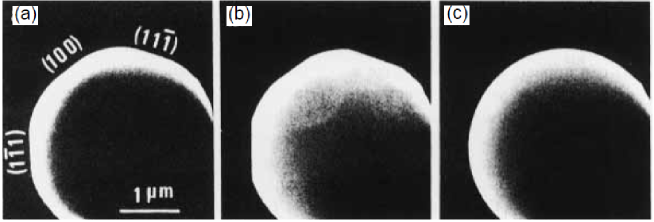
Figure C.1: SEM image of Pb crystal at equilibrium viewed from the [011] azimuth for (a) $300\,^{\circ}\mathrm{C}$, (b) $320\,^{\circ}\mathrm{C}$ and (c) $327\,^{\circ}\mathrm{C}$, above the Pb melting point. Extracted from [3].

The shape of an object at the equilibrium can be predicted by variational principle of the suitable thermodynamic potential [3]. For a crystal, the surface tension depends on what face is considered and $\gamma=\gamma(hkl,T)$, where $hkl$ are the Miller’s indices. This anisotropy governs the crystal shape and, as the temperature increases, it tends to be minimized [4]. Above the melting point, the anisotropy vanishes and the material must recover the spherical form [3, 4]. In the fig. C.1 one can seen equilibrium shapes for Pb crystals at different temperatures. As temperature increases the anisotropy decreases and fewer facets are formed. Above the melting point, where Pb is liquid, the spherical shape is achieved.

C.2   Nucleation

Nucleation is a fundamental process happening during a phase transition [2]. It is important for thin films because the structures appearing in the submonolayer regime strongly affects the dynamic of the growth [23, 160]. Simple models for nucleation are based on the liquid drop model, which also works for solids. The basic difference is that solids have two additional features: elasticity and commensurability [4]. These effects will be discussed along this section. Nucleation models are important just as a qualitative fashion once one deals with few atoms and, hence, a continuum description (on thermodynamic basis) of the phenomenon becomes doubtful [2].

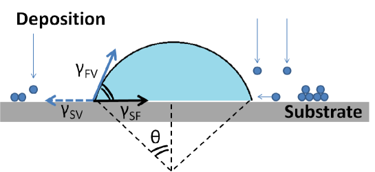
Figure C.2: Schematic of nucleation processes in a gas-to-solid phase transition.

Consider a possible heterogeneous nucleation of a condensed film on a crystalline substrate (see a scheme in the fig. C.2). Deposition can occurs solely if the vapor is supersaturated ($S_{s}>0$). It means there exist a $\Delta P$ driving the atoms toward the substrate. The eq. C.1 summarizes this condition:

$$\Delta G_{v}=-\frac{K_{B}T}{V_{a}}\ln(1+S_{s}),$$ (C.1)

where $\Delta G_{v}$ is the change in the free energy per unit volume; $K_{B}$ is the Boltzmann constant; $V_{a}$ the atomic volume; and $S_{s}\equiv\frac{P_{V}-P_{S}}{P_{S}}$ is the vapor supersaturation with $P_{V}-P_{S}$ being the difference between pressures of the vapor and above the solid, respectively.

The molecules (or atoms) impinge onto the substrate and produce, in a reasonable approximation, spherical nucleus of mean radius $r$. The change $\Delta G$ for the substrate-film system is due to three contributions: (1) the first associated with all bonds to create the nucleus ($\sim r^{3}\Delta G_{v}$); (2) a superficial film/vapor term owing the new nucleus ($\sim r^{2}\gamma_{fv}$); (3) and the contribution emerging from the difference between the energy at the old substrate/vapor surface ($\sim r^{2}\gamma_{sv}$) and at the new substrate/film interface ($\sim r^{2}\gamma_{sf}$). It reads:

$$\triangle G=a_{1}r^{3}\triangle G_{v}+a_{2}r^{2}\gamma_{fv}+a_{3}(r^{2}\gamma_{fs}-r^{2}\gamma_{sv}),$$ (C.2)

where $a_{1}=\frac{\pi}{3}(2-3cos\theta+cos^{3}\theta)$; $a_{2}=2\pi(1-cos\theta)$; $a_{3}=\pi sen^{2}\theta$; and $\theta$ is the wetting angle.

In the fig. C.3 there is a plot of $\Delta G$ as function of $r$. At an instable equilibrium point, $\frac{d\Delta G}{dr}=0$, there is a critical nucleus size, $r^{*}$, from which island growth becomes energetically favorable. In other words, at least an amount of $\Delta G^{*}=\Delta G(r^{*})$ energy must be supplied to the system for triggering spontaneous growth, where the nucleus size grows indefinitely.

An important question raises up: How islands reach the stable size, since for $r<r^{*}$ they tend to shrink? One must to take into account that theses processes are stochastic and thermal fluctuations ($K_{B}T\approx\Delta G^{*}$) are responsible to yield a density $N^{*}$ of stable islands per unit time. Assuming a Boltzmann statistic, then $N^{*}\sim exp[-\Delta G^{*}/K_{B}T]$. Since $\Delta G^{*}$ must be function of T and of the molecular flux F [atoms$/cm^{2}s$], one can get the feeling about how these parameters affect nucleation processes.

Figure C.3: Qualitative change of the free energy as function of the mean nucleus size during a gas-to-solid phase transition.

C.2.1   Nucleation dependence on substrate temperature

It is reasonable that molecular flux is directly related to $S$ such that one can replace $1+S_{s}$ by $F/F_{e}$ in the eq. C.1, with $F_{e}$ being the evaporation rate from the film at equilibrium. Inserting this in $\Delta G$ and extracting $r^{*}$ from the instable equilibrium point, one can show (considering $\partial\gamma/\partial T\approx 0$ N/mK [2]):

$$(\partial r^{*}/\partial T)_{|_{F}}\sim[a_{2}\gamma_{fv}+a_{3}(\gamma_{fs}-\gamma_{sv})]/T^{2}.$$ (C.3)

At this point it is clear that the behavior of the critical size, as function of T, depends on the relationship between the surface tensions. Indeed, this relationship is also used to describe growth modes of films (see next section). For instance, taking the simplest situation, where $\gamma_{fs}\approx\gamma_{sv}$, one has $(\partial r^{*}/\partial T)_{|_{F}}>0$. Hence, locally, mean critical size of the islands becomes larger as temperature increases (at least for a range of T, because the result $\sim 1/T^{2}$). By using the same procedure one can also find:

$$\partial(\Delta G^{*})/\partial T)_{|_{F}}>0,$$ (C.4)

likewise $r^{*}$, the energy barrier $\Delta G^{*}$ increases as T increases. This result implies that the nucleation rate is reduced exponentially in accordance with the Boltzmann statistic. Qualitatively, theses results have already been found in the classical work on supercooled liquid tin and water drops, backing to the 1950’s [178]. The crystallizations of synthetic granite and granodiorite [179], as well as the famous growth of Si on Si(001) [180] agree with those results. However, there are also examples going in the opposite direction. S. O. Ferreira et al. [9, 10] have explored direct three-dimensional island formation in the growth of CdTe on Si(111) substrates for showing that the Quantum-Dots (QD’s) density increases with T in the range of 200 to $300\,^{\circ}\mathrm{C}$, whilst the mean QD’s size decreases (fig. C.4).

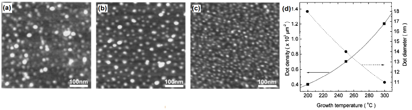
Figure C.4: Atomic force microscopy images of CdTe Quantum-Dots grown by HWE on Si(111) substrates at (a) $200\,^{\circ}\mathrm{C}$, (b) $250\,^{\circ}\mathrm{C}$, and (c) $300\,^{\circ}\mathrm{C}$. (d) Dot density ($\blacksquare$) and diameter (•) as function of T. Courtesy of Prof. S. O. Ferreira. These results can be found in the Ref. [9, 10].

C.2.2   Nucleation dependence on molecular flux

Once one has $r^{*}=r^{*}(T,F)$, it is straightforward showing the dependence on $F$ at T constant. Considering the same simplest situation, one reaches to:

$$(\partial r^{*}/\partial F)_{|_{T}}<0\qquad\textrm{and }\qquad[\partial(\Delta G^{*})/\partial F]_{|_{T}}<0.$$ (C.5)

Eq. C.5 tells us that nuclei size are smaller as the molecular flux increases, but at the same time, the nucleation rate is bigger. This result agree with the intuitive feeling that when more particles arrive onto substrate per unit time there is no time enough for the particles find an already stable island where they can pile up. Consequently, it is likely they form dimers and other instable small islands. These results match, for instance, with those reported for the growth of InAs/GaAs QD’s on GaAs(001) substrates by MBE [183]. At $T=490\,^{\circ}\mathrm{C}$ and $F=0.016$ ML $s^{-1}$, the QD’s density is about $0.2\times 10^{11}$ $cm^{-2}$ and their diameter is near from 200 Å. However, as $F$ is increased to $0.094$ ML $s^{-1}$, at fixed temperature, the QD’s density also increases at least five times, whereas the QD’s diameter goes to about 150 Å.

Studies converging in this vein (and related to them) can be found in the cap. 9 of the Ref. [160] as well as in the already cited Refs. [178, 179, 180, 9, 10, 183] and Refs. therein.

C.3   Growth and structure of films

C.3.1   Growth Modes

The mechanical equilibrium condition (eq. C.6), predicted by the drop liquid model, provide a reasonable way to explain three basic growth modes for solids.

$$\gamma_{sv}=\gamma_{sf}+\gamma_{fv}\cos{\theta}.$$ (C.6)

When the film “wets” the whole substrate surface, nucleating two-dimensional islands on the interface, then $\theta\cong 0$ and $\gamma_{sv}\geq\gamma_{sf}+\gamma_{fv}$. This is the called Frank-van der Merwe (FM) or layer-by-layer growth mode, often observed in metal deposited on metal and homoepitaxial growth [2]. In this mode, ideally, the subsequent layer starts growing just after the complete formation of the precedent layer.

Otherwise, when there is not the “wetting layer” and three-dimensional islands are nucleated directly on the substrate, the Volmer-Weber (VW) growth mode takes place. In this situation parts of the substrate remain exposed and the energy is minimized reducing the film/vapor interface, since $\gamma_{fv}\gg\gamma_{sv}+\gamma_{sf}$. CdTe grown on Si(111) (fig. C.4), for instance, follows this kind of growth [9, 10].

Lastly, the Stranski-Krastanov (SK) growth mode is understood as a transition between FM to VW mode [2]. At the first 3-5 monolayers of deposition, $\gamma_{sv}$ dominates growth making wetting. After that, direct three-dimensional islands start to nucleate on the subsequent layers. Any energetic disturb (defects, accumulated strain, etc.) can be the origin of this transition [2, 3, 4]. A typical example of SK growth mode occurs in Ge films deposited on Si(001), where a metastable phase containing small clusters precedes the “macroscopic” three-dimensional growth. See the fig. C.5 [184].

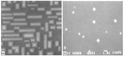
Figure C.5: Ge films grown on Si(001) through SK mode. (a) Scanning Tunneling Microscopy (STM) 2500 x 2500 Å image of “hut” Ge clusters on Ge layers grown in the FM growth mode. The clusters are $\lesssim$ 1000 Å long and 20-40 Å high. One believes that this is a signature preceding macroscopic three-dimensional nucleations. (b) SEM image of the subsequent growth dominated by the macroscopic three-dimensional Ge islands. These clusters are $\sim$ 250 Å high and much larger than the hut clusters, which can not be viewed in this scale. Images extracted and edited from [184].

It is very important mention that the growth mode depends not only on the materials involved in the process, but mainly on the growth parameters, including whether impurities are present. The growth of Ag on Ag(111) in the range of temperature from 175 to 575 K, for instance, changes gradually from three-dimensional (VW) to step-flow growth. However, if submonolayer deposits of Sb are present, so the growth behavior becomes layer-by-layer (FM) over the entire range of 225K to 375 K [185].

C.3.2   Commensurability and Polycrystallinity

During a nucleation, under very special conditions, the film can “copy” the substrate crystalline structure [2]. In these cases, one says that the growth is commensurate or epitaxial [4]. Several semiconductor devices depends on epitaxy. The most commons are optoelectronic ones, as LEDs and lasers based on GaInN materials, and those used in high-speed microelectronic digital (wireless communications), composed of Ge_xSi_1-x [2]. Typically, the first step in epitaxial films is the homo-epitaxial Si on Si growth by CVD. The reason is that the epilayer is free from defects, purer than the wafer and can be doped independently of it.

Epitaxy depends on the mismatch between the lattice parameters ($|a_{f}-a_{s}|/a_{s}$) of the film ($a_{f}$) and of the substrate ($a_{s}$), including their thermal dependence via the dilatation coefficient [156, 157, 151]. It occurs whether the relative mismatch is below $\approx 10-15\%$ [156, 157]. Nevertheless, exotic cases (called hard epitaxy) as the hetero-epitaxial CdTe layers grown on Si(111) also exist [154], in spite of almost $19\%$ and $48\%$ mismatch of the lattice parameter and thermal coefficient, respectively. Larger mismatch implies larger accumulated strain (elastical energy) which can be released as defects or can support a transition from FM to VW growth mode.

It is worth mention that the effect of heteroepitaxy can be included in the drop liquid model replacing the term ($\sim\Delta G_{v}$) by $[\sim(\Delta G_{v}+\Delta G_{s})]$ in the eq. C.2, where $\Delta G_{s}$ inserts the extra energy accumulated in the strain form. $\Delta G^{*}$ increases leading the nucleation rate to decline. Other effects as impurities, defects, chemical reactions also can be inserted into the model in order to get the felling about their consequences on nucleations [2].

Unlike epitaxial single-crystals, polycrystalline films are composed by an collection of grains, each of them having its own crystallographic orientation. These environments lead to a complex competition between neighboring grains which are droved by the surface tensions, once $\gamma=\gamma(hkl)$ [2, 3, 4]. Generally, a preferential direction of growth ($\Lambda$), called texture [2, 151, 186], appears and evolves as deposition proceeds. Grains_Λ grow faster than the others and, eventually, dominate the surface. Texture affects mechanical and electrical features of films, including their elastic modulus, yield strength, magnetic permeability, etching rate, diffusion rate, and others [2]. Standard procedure quantifying texture is based on X-ray diffraction techniques [186, 151].

C.4   Kinetic Phenomena and Superficial Structures

Crystal (surface) growth is a far-from-equilibrium phenomenon. During a growth from vapor phase, atoms impinge onto the substrate (interface) breaking and/or forming local bonds, changing the morphology and hampering the system to minimize its free energy [160]. As the substrate is heated, the adosrbed atoms, or molecules, (called adatoms) might diffuse on the surface performing Brownian motions. Commonly, these adatoms stick at positions which maximize their number of coordination and deposition occurs [2]. Thermal fluctuation may also induces desorption, i.e, adatoms leave the surface, returning to the vapor [23]. Deposition, desorption and aggregation mediated by diffusion are the basic mechanisms ruling a general growth. Of course, specific situations excludes one, maybe two of these processes, but we are considering the wide case. These last two, and other cited below, are thermally activated, namely, they occur with rates given by Arrhenius’ laws (eq. C.7) [2, 3, 4, 23]:

$$\tau=\tau_{0}\exp{[-E_{\tau}/K_{B}T]},$$ (C.7)

where $\tau$ is a rate of a particular event, $\tau_{0}$ a constant, and $E_{\tau}$ is the energy associated with the $\tau$ process.

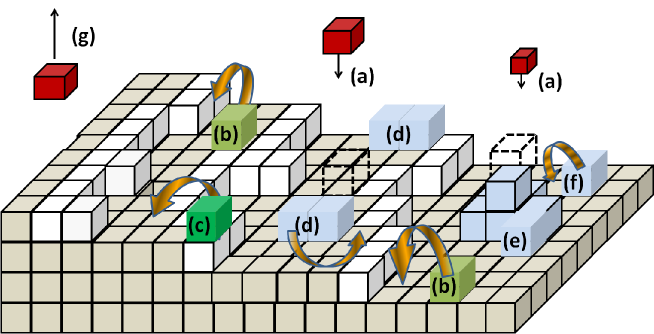
Figure C.6: Schematic of kinetic processes occurring during the growth.

A crystal surface is not a perfect plane. Indeed, it presents large pieces (terraces) separated by steps of atomic height (or multiples of an atomic heigth) - see and follow the fig. C.6. Even theses steps are not perfectly straight, rather they contain straight parts separated by kinks [4]. Particles arriving at the substrate (a) have an amount of energy relative to the vapor phase [3]. They use this energy for breaking chemical bonds already established at surface and/or for becoming adatoms (b). Adatoms diffuse with a rate $\tau_{diff}$, since that, for each hop, an adatom must overcome the lattice potential existing between neighboring positions (see fig. C.7). This potential depends on the nature of compounds involved in the growth and on the substrate face.

Preferential sites for sticking are the edge of steps and kinks, once they have a larger number of dangling bonds [4]. However, adatoms reach these positions only if the temperature is sufficiently high for promoting a length diffusion ($x_{diff}$) comparable to the terrace separation length ($x_{terr}$) [3]. Step-flow growth is achieved when $x_{diff}\gg x_{terr}$ [4]. Interestingly, if an adatom diffuses on a terrace, but towards another one (c), it tends to come back instead to jump off the terrace. This is known as Ehrlich-Schowoebel effect (ES) [181, 160]. In the fig. C.7 the effect of the ES barrier is added. In cases where the ES barrier dominates the growth (see Pt grown on Pt(111), fig. 102 in the ref. [160]) structures looking like wedding cakes are formed [160]. Among several ways to define an expression for the diffusion energy that includes the ES barrier, one usually employed is:

$$E_{diff}=E_{0}+nE_{n}+E_{es},$$ (C.8)

where $n$ is the number of coordination; $E_{n}$ is the energy per unit bond and $E_{es}$ is the associated energy to the ES barrier. Typically, $E_{n}\sim 0.1$ eV and $E_{es}\sim 0.01$ eV [23]. However, it is worth keep in mind that these values may change appreciably depending on the system considered. Additionally, the eq. C.8 is solely a simplified model which does not catch all source of energies involved in real processes.

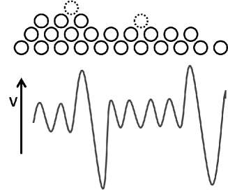
Figure C.7: Schematic of the lattice potential.

Since an adatom establishes bonds, deposition happens. When an adatom meets another atom, they can form a dimer (d). Dimers also diffuse, albeit it is (much)less probable due to the enhance of $E_{diff}$. Sometimes, dimers grow and become a two- or three-dimensional island (e), which tend to capture adatoms (f) (if $r>r^{*}$). At the same time, some atoms break off their bonds and leave the surface (g). So, desorption occurs. Desorption is an effect competing with deposition. Due to this effect, the molecular flux migth be different from the deposition rate. However, in usual MBE (and related technique) conditions, desorption is a neglegible process [2, 3, 4, 23]. For Ga on GaAs(111) over the range 860K to 960 K, the desorption energy is $E_{des}\approx 2.5$ eV [23]. Assuming $1/\tau_{0des}=10^{-14}$ s and $T=850$ K in the inverse of eq. C.7, one obtains that only one Ga atom is desorbed from the surface in each 2 $s$. Comparing this desorption rate with the deposition rate used in MBE ($\sim 10^{16-18}$ atoms $cm^{-2}$ $s^{-1}$), it eases to see that desorption phenomenon is inoperative [23].

List of Acronyms and Symbols

Acronyms

Acronym	Description
AFM	Atomic Force Microscopy
BD	Ballistic Deposition
CF	Correlation Function
CRSOS	Conserved Restricted Solid-On-Solid
CVD	Chemical Vapor Deposition
DI	Deionized
DPRM	Directed Polymer in a Random Medium
DT	Das-Sarma-Tamborenea
EVS	Extreme-Value Statistics
EW	Edwards-Wilkinson
FM	Frank-van-der-Merwe
FV	Family-Vicsek
GBs	Grain Boundaries
GOE	Gaussian Orthogonal Ensemble
GPS	Global Position System
GUE	Gaussian Unitary Ensemble
H	Height of “grains” used as parameter in a Kinetic Monte Carlo Model
HDs	Height Distributions
HWE	Hot Wall Epitaxy
IC	Initial Conditions
KPZ	Kardar-Parisi-Zhang
LEDs	Light Emission Diodes
MBE	Molecular Beam Epitaxy
MH	Mullins-Herring
ML	Mono-Layer
MRHDs	Maximal Relative Height Distributions
pdf	probability density function
PNG	Poly-Nuclear-Growth
QDs	Quantum Dots
RDSR	Random Deposition with Surface Relaxation
RSOS	Restricted Solid-On-Solid
SEM	Scanning Electron Microscopy
SK	Stranski-Krastanov
SLRDs	Squared Local Roughness Distributions
STM	Scanning Tunelling Microscopy
TASEP	Totally Asymetric Exclusion Process
TW	Tracy-Widom
UC	Universality Class
VLDS	Villain-Las-Das-Sarma
VW	Volmer-Weber
WV	Wolf-Villain
XPS	X-ray Photoelectron Spectroscopy
XRD	X-Ray Diffraction

Symbols

Latin Symbols	Description
$a_{f}$	Lattice parameter of the film
$a_{s}$	Lattice parameter of the substrate
$A$	Static amplitude in the KPZ context
$A_{f}$	Area of a film
$A_{\theta-2\theta}$	Absortion factor for a $\theta-2\theta$ XRD geometry
$C_{h}$	Heigth-difference correlation function
$C_{s}$	Spatial covariance
$d$	Dimension of a growth process
$d_{s}$	Substrate dimension
$\sqrt{D}$	Amplitude of the white noise
$E_{0}$	Enery of the lattice potential
$E_{diff}$	Characteristic energy of diffusion
$E_{es}$	Ehrlich-Showoebel barrier energy
$E_{gap}$	Energy gap
$E_{n}$	Energy per unit bond
$E_{GB}$	Energy barrier at GBs of colided neighboring grains
$E_{R}$	Relaxation energy barrier at the GBs of colided neighboring grains
$E_{\tau}$	Energy of a particular kinetic effect
$F$	Molecular Flux
$F_{0}$	Baik-Rains distribution
$F_{e}$	Evaporation rate from the film at equilibrium
$F_{H}$	Helmholtz free energy
$G$	Gibbs free energy
$G_{s}$	Gibbs free energy related to strain
$G_{v}$	Gibbs free energy per unit volume
$G^{*}$	Critical gibbs free energy
$G(X;m)$	Gumbel pdf of the X variable; m-th order
$h_{i}$	Surface height at the site i
$h(x,t)$	Surface height at the substrate position $x$ at time t
$\langle h^{n}\rangle_{c}$	n-th cumulant of h
ĥ	Surface height in the reciprocal space
$I_{111}$	Intensity of the (111) peak in a XRD spectrum
$j$	Current density
$J$	Current density parallel to the surface
$K$	Kurtosis coefficient
$K_{d}$	Strength of diffusion
$K_{B}$	Boltzman constant
$l^{*}$	Characteristic box size
$L$	Lateral size of the substrate
$m_{n}$	nth-moment of a pdf
$m^{*}$	Maximal height relative to the mean height of an interface
$n_{coar}$	Coarsening exponent
$N_{h}$	Number of points at the surface with height h
$N^{*}$	Density of stable islands per unit time
$p(h)$	Density probability of the variable $h$
p̃$(k)$	Characteristic function
$P$	Pressure
$P_{D}$	Probability of particle diffusing towards a defect site
$P_{R}$	Probability of ocurring a relaxation process at GBs
$P_{S}$	Pressure above vapor the solid
$P_{V}$	Pressure of the vapor phase
$P(h)$	Probability of the variable $h$
$Q$	Generalized thermodynamic force
$r$	Mean radius of a quasi-spherical nucleus
$r_{c}$	Average grain size
$r_{m}$	First minimum/zero of the Slope-Slope spatial covariance
$r^{*}$	Critical size of an island
$R$	Local curvature
$S$	Skewness coefficient
$\overleftrightarrow{S}$	Space-time referential
$S(k,t)$	Structure factor or Power-spectrum
$S_{s}$	Supersaturation
$t$	Growth time
$th$	Thickness of a thin film
$t_{x}$	Crossover time
$T$	Temperature of the substrate
$T_{EW}$	Substrate temperature corresponding to an EW growth
$T_{EW-KPZ}$	Substrate temperature corresponding to an EW-to-KPZ crossover
$v$	Average growth velocity of an interface
$v_{\infty}$	Asymptotic growth velocity of an interface
$V$	Volume
$V_{a}$	Atomic volume
$w_{loc}$	Local roughness
$w_{sat}$	Saturation value for the roughness
$w(L,t)$	Global roughness
$W$	Thermodynamical work
$x_{diff}$	Characteristic length for diffusion
$x_{diff}$	Length of a terrace
$z$	Dynamic exponent
Greek Symbols	Description
$\alpha$	Roughness exponent
$\alpha_{1}$	Geometrical exponent
$\alpha_{s}$	Spectral roughness exponent
$\gamma$	Surface energy or Surface tension
$\gamma_{fv}$	Surface tension at the film-vapor interface
$\gamma_{p}$	Non-universal parameter in the KPZ scaling theory context
$\gamma_{sf}$	Surface tension at the substrate-film interface
$\gamma_{sv}$	Surface tension at the substrate-vapor interface
$\Gamma$	Non-universal parameter in the KPZ scaling theory context
$\Gamma_{f}$	Gamma function
$\Gamma(l,t)$	Slope-Slope spatial covariance
$\epsilon$	Tilting angle
$\zeta$	Characteristic length in the surface
$\zeta_{p}$	Non-universal parameter in the KPZ scaling theory context
$\eta$	Noise
$\eta_{p}$	Non-universal parameter in the KPZ scaling theory context
$\theta_{hkl}$	Wetting angle
$\theta_{hkl}$	Angle of reflection for the (hkl) peak in a XRD measurement
$\Theta$	Functional of x, h and t
$\kappa$	Kappa exponent
$\lambda$	Excess of velocity of an interface
$\lambda_{Cu_{K\alpha}}$	Wavelenght of the radiation in a Kα transition for a Cu atom
$\Lambda$	Preferential direction of growth - Texture direction
$\mu$	Chemical potential
$\mu_{v}$	Chemical potential in a vapor phase
$\nu$	Strength of the “surface tension”
$\xi$	Correlation length
$\xi_{||}$	Parallel correlation length
$\Xi$	Grand potential
$\sigma_{h}$	Standard deviation of h
$\sigma_{\chi}$	Standard deviation of $\chi$
$\varsigma$	Scale factor
$\tau$	Rate of a particular kinetic effect
$\tau_{0des}$	Rate of desorption
$\tau_{diff}$	Rate of diffusion
$\Phi$	Universal scaling function
$\chi$	Random variable
$\langle\chi\rangle$	Mean of $chi$
$\langle\chi^{2}\rangle_{c}$	Second cumulant of $\chi$
$\psi_{k}$	Polygamma function of kth-order
$\Psi$	Universal scaling function
$\Omega$	Aspect ratio of a grain/mound

References

- [1]
- [2] M. Ohring, Materials science of thin films. Academic press (2001).
- [3] J. A. Venables, Introduction to surface and thin film processes. Cambridge University Press (2000).
- [4] A. Pimpinelli, J. Villain, Physics of crystal growth. Cambridge University Press (1999).
- [5] R. Triboulet, P. Siffert, CdTe and Related Compounds: Physics, Defects, Hetero- and Nano-structures, Crystal Growth, Surfaces and Applications. Elsevier Science (2009).
- [6] L. Chen, Y. Wu, J. Poplawsky, T. J. Pennycook, N. Paudel, W. Yin, S. J. Haigh, M. P. Oxley, A. R. Lupini, M. Al-Jassim, S. J. Pennycook, Y. Yan, “Grain-Boundary-Enhanced Carrier Collection in CdTe Solar Cells”, Phys. Rev. Lett. 112, 156103 (2014).
- [7] J. Rams, N. V. Sochinskii, V. Munõz, J. M. Cabrera, “CdTe epilayers for uses in optical waveguides”, Appl. Phys. A 71, 277 (2000).
- [8] L. Manna, D. J. Milliron, A. Meisel, E. C. Scher, A. P. Alivisatos, “Controlled growth of tetrapod-branched inorganic nanocrystals”, Nature Materials 2, 382 (2003).
- [9] S. O. Ferreira, E. C. Paiva, G. N. Fontes, B. R. A. Neves, “Characterization of CdTe quantum dots grown on Si(111) by hot wall epitaxy”, J. Appl. Phys. 93, 1195 (2003).
- [10] J. Suela, I. R. B. Ribeiro, S. O. Ferreira, A. Malachias, G. N. Fontes, L. A. Montoro, A. J. Ramirez “Evolution of crystalline domain size and epitaxial orientation of CdTe/Si(111) quantum dots”, J. Appl. Phys 107, 064305 (2010).
- [11] B. L. Williams, D. P. Halliday, B. G. Mendis, K. Durose, “Microstructure and point defects in CdTe nanowires for photovoltaic applications”, Nanotechnology 24, 135703 (2013).
- [12] M. Saba, C. Ciuti, J. Bloch, V. Thierry-Mieg, R. André, L. S. Dang, S. Kundermann, A. Mura, G. Bongiovanni, J. L. Staehli, B. Deveaud, “High-temperature ultrafast polariton parametric amplification in semiconductor microcavities”, Nature (London) 414, 731 (2001).
- [13] S. O. Ferreira, I. R. B. Ribeiro, J. Suela, I. L. Menezes-Sobrinho, S. C. Ferreira, S. G. Alves, “Effect of temperature on the Hurst and growth exponents of CdTe polycrystalline films”, Appl. Phys. Lett. 88, 244102 (2006).
- [14] I. R. B. Ribeiro, J. Suela, J. E. Oliveira, S. O. Ferreira, P. Motisuke, “Low temperature growth of high quality CdTe polycrystalline layers”, J. Phys. D: Appl. Phys. 40, 4610 (2007).
- [15] A. S. Mata, S. C. Ferreira, I. R. B. Ribeiro, S. O. Ferreira, “Anomalous scaling and super-roughness in the growth of CdTe polycrystalline films”, Phys. Rev. B 78, 115305 (2008).
- [16] F. S. Nascimento, S. C. Ferreira, S. O. Ferreira, “Faceted anomalous scaling in the epitaxial growth of semiconductor films”, Europhys. Lett. 94, 68002 (2011).
- [17] H. Assender, V. Bliznyuk, K. Porfyrakis, “How Surface Topography Relates to Materials’ Properties”, Science 297, 973 (2002).
- [18] D. Siniscalco, M. Edely, J. F. Bardeu, N. Delorme, “Statistical Analysis of Mounded Surfaces: Application to the Evolution of Ultrathin Gold Film Morphology with Deposition Temperature”, Langmuir 29, 717 (2013).
- [19] M. Kardar, Statistical physics of fields. Cambridge University Press (2007).
- [20] A. -L. Barabási, R. Albert, “Emergence of scaling in random networks”, Science 286, 509 (1999).
- [21] J. P. Sethna, K. A. Dahmen, C. R. Myers, “Crackling noise”, Nature 410, 242 (2001).
- [22] C. Castellano, S. Fortunato, V.Loreto, “Statistical physics of social dynamics”, Rev. of Modern Phys. 81, 591 (2009).
- [23] A. -L. Barabási, H. E. Stanley, Fractal concepts in surface growth. Cambridge university press (1995).
- [24] B. B. Mandelbrot, The fractal geometry of nature. Times Books, (1983).
- [25] M. Kardar, G. Parisi, Y. -C. Zhang, “Dynamic scaling of growing interfaces”, Phys. Rev. Lett. 56, 889 (1986).
- [26] T. Halpin-Healy, Y. -C. Zhang, “Kinetic roughening phenomena, sthocastic growth, directed polymers and all that: Aspects of multidisciplinary statistical mechanics”, Phys. Rep. 254, 215 (1995).
- [27] I. Corwin, “The Kardar-Parisi-Zhang Equation and Universality Class”, Theory Appl., 01, 1130001 (2012).
- [28] K. Johansson, “Shape Fluctuations and Random Matrices”, Comm. Math. Phys. 209, 437 (2000).
- [29] M. Prähofer, H. Sphon, “Universal Distributions for Growth Process in 1 + 1 Dimensions and Random Matrices”, Phys. Rev. Lett. 22, 4882 (2000).
- [30] C. A. Tracy, H. Widom, “Level-spacing distributions and the Airy kernel”, Commun. Math. Phys. 159, 151 (1994); 77, 727 (1996).
- [31] C. A. Tracy, H. Widom, “On orthogonal and symplectic matrix ensenbles”, Commun. Math. Phys. 77, 727 (1996).
- [32] M. Kardar, “Comment on the Roughening by impurities at finite temperatures”, Phys. Rev. Lett. 55, 2923 (1985).
- [33] T. Sasamoto, H. Spohn, “One-Dimensional Kardar-Parisi-Zhang Equation: An Exact Solution and its Universality”, Phys. Rev. Lett. 104, 230602 (2010).
- [34] G. Amir, I. Corwin, J. Quastel, “Probability distribution of the free energy of the continuum directed random polymer in 1 + 1 dimensions”, Commun. Pure Appl. Math. 64, 466 (2011).
- [35] P. Calabrese, P. Le Doussal, A. Rosso, “Free-energy distribution of the directed polymer at high temperature”, Europhys. Lett. 90, 20 002 (2010).
-
[36]
V. Dotsenko, “Bethe ansatz derivation of the Tracy-Widom distribution for one-dimensio-
nal directed polymers”, Europhys. Lett. 90, 20 003 (2010). - [37] P. Calabrese, P. Le Doussal, “Exact Solution for the Kardar-Parisi-Zhang Equation with Flat Initial Conditions”, Phys. Rev. Lett. 106, 250603 (2011).
- [38] T. Imamura, T. Sasamoto, “Exact Solution for the Stationary Kardar-Parisi-Zhang Equation”, Phys. Rev. Lett. 108, 190603 (2012).
- [39] K. A. Takeuchi, M. Sano, “Universal Fluctuations of Growing Interfaces: Evidence in Turbulent Liquid Crystals”, Phys. Rev. Lett. 104, 230601 (2010).
- [40] K. A. Takeuchi, M. Sano, T. Sasamoto, H. Sphon, “Growing interfaces uncover universal fluctuations behind scale invariance”, Sci. Rep. 1, 34 (2011).
- [41] K. A. Takeuchi, “Crossover from Growing to Stationary Interfaces in the Kardar-Parisi-Zhang Class”, Phys. Rev. Lett. 110, 210604 (2013).
- [42] K. A. Takeuchi, M. Sano, “Evidence for Geometry-Dependent Universal Fluctuations of the Kardar-Parisi-Zhang Interfaces in Liquid-Crystal Turbulence”, J. Stat. Phys. 147, 853 (2012).
- [43] J. Maunuksela, M. Myllys, O. -P. Kähkönen, J. Timonen, N. Provatas, M. J. Alava, and T. Ala-Nissila, “Kinetic Roughening in Slow Combustion of Paper” , Phys. Rev. Lett. 79, 1515 (1997).
- [44] M. Myllys, J. Maunuksela, M. J. Alava, T. Ala-Nissila, and J. Timonen, “Scaling and Noise in Slow Combustion of Paper”, Phys. Rev. Lett. 84, 1946 (2001).
- [45] M. Myllys, J. Maunuksela, M. Alava, T.Ala-Nissila, J. Merikoski, and J. Timonen, “Kinetic roughening in slow combustion of paper”, Phys. Rev. E 64, 036101 (2001).
- [46] J. Merikoski, J. Maunuksela, M. Myllys, and J. Timonen, “Temporal and Spatial Persistence of Combustion Fronts in Paper”, Phys. Rev. Lett. 90, 024501 (2003).
- [47] P. J. Yunker, M. A. Lohr, T. Still, A. Borodin, D. J. Durlan, and A. G. Yodh, “Effects of Particle Shape on Growth Dynamics at Edges of Evaporating Drops of Colloidal Suspensions”, Phys. Rev. Lett. 110, 035501 (2013).
- [48] S. G. Alves, T. J. Oliveira, S. C. Ferreira, “Universal Fluctuations in radial growth models belonging to the KPZ universality class”, Europhys. Lett. 96, 48003 (2011)., J. Stat. Mech. 2013, 05007 (2013).
- [49] T. J. Oliveira, S. C. Ferreira, S. G. Alves, “Universal fluctuations in Kardar-Parisi-Zhang growth on one-dimensional flat substrates”, Phys. Rev. E 85, 010601(R) (2012).
- [50] S. Prolhac, H. Sphon, “Height distribution of the Kardar-Parisi-Zhang equation with sharp-wedge initial condition: Numerical evaluations”, Phys. Rev. E 84, 011119 (2011).
- [51] T. Halpin-Healy, Y. Lin, “Universal aspects of curved, flat, and stationary-state Kardar-Parisi-Zhang statistics”, Phys. Rev. E 89, 010103(R) (2014).
- [52] J. Kelling, G. Ódor, “Extremly large-scale simulation of a Kardar-Parisi-Zhang model using graphics cards”, Phys. Rev. E 84 061150 (2011).
- [53] E. Marinari, A. Pagnani, G. Parisi, “Critical exponents of the KPZ equation via multi-surface coding numerical simulations”, J. Phys. A: Math. Gen. 33, 8181 (2000).
- [54] F. D. A. Aarão Reis, “Universality in two-dimensional Kardar-Parisi-Zhang growth”, Phys. Rev. E 69, 021610 (2004).
- [55] Z. Rácz, M. Plischke, “Width distribution for (2+1)-dimensional growth and deposition processes”, Phys. Rev. E 50, 3530 (1994).
- [56] E. Marinari, A. Pagnani, G. Parisi, Z. Rácz, “Width distributions and the upper critical dimension of Kardar-Parisi-Zhang interfaces”, Phys. Rev. E 65, 026136 (2002).
- [57] T. J. Oliveira, F. D. A. Aarão Reis, “Maximal- and minimal-height distributions of fluctuating interfaces”, Phys. Rev. E 77, 041605 (2008).
- [58] T. Halpin-Healy, “(2+1)-Dimensional Directed Polymer in a Random Medium: Scaling Phenomena and Universal Distributions”, Phys. Rev. Lett. 109, 170602 (2012).
-
[59]
T. Halpin-Healy, “Extremal paths, the stochastic heat equation, and the three-dimensio-
nal Kardar-Parisi-Zhang universality class”, Phys. Rev. E 88, 042118 (2013). - [60] T. J. Oliveira, S. G. Alves, S. C. Ferreira, “Kardar-Parisi-Zhang universality class in (2+1) dimensions: Universal geometry-dependent distributions and finite-time corrections” Phys. Rev. E 87, 040102(R) (2013).
- [61] I. S. S. Carrasco, K. A. Takeuchi, S. C. Ferreira, T. J. Oliveira, “Interface fluctuations for deposition on enlarging flat substrates”, New J. Phys. 16, 123057 (2014).
- [62] F. Ojeda, R. Cuerno, R. Salvarezza, and L. Vázquez, “Dynamics of Rough Interfaces in Chemical Vapor Deposition: Experiments and a Model for Silica”, Phys. Rev. Lett. 84, 3125 (2000).
- [63] See the references [7] in Ojeda F. et al., Phys. Rev. Lett. 84, 3125 (2000).
- [64] R. A. L. Almeida, S. O. Ferreira, T. J. Oliveira, F. D. A. Aarão Reis, “Universal fluctuations in the growth of semiconductor thin films”, Phys. Rev. B 89, 045309 (2014).
- [65] T. Halpin-Healy, G. Palasantzas, “Universal correlators distributions as experimental signatures of 2 + 1 dimensional Kardar-Parisi-Zhang growth”, Europhys. Lett. 105, 50001 (2014).
- [66] R. Cuerno, L. Vázquez, “Universality issues in surface kinetic roughening of thin solid films.”, arXiv preprint cond-mat/0402630 (2004).
- [67] M. Schroeder, M. Siegert, D. E. Wolf, J. D. Shore, and M. Plischke, “Scaling of Growing Surfaces with Large Local Slopes”, Europhys. Lett. 24, 563 (1993).
- [68] J. M. López, M. A. Rodríguez, “Lack of self-affinity and anomalous roughening in growth processes”, Phys. Rev. E 54, R2189 (1996).
- [69] J. M. López, M. A. Rodriíguez, R.Cuerno, “Superroughening versus intrinsic anomalous scaling of surfaces”, Phys. Rev. E 56, 3993 (1997).
- [70] J. M. López, “Scaling Approach to Calculate Critical Exponents in Anomalous Surface Roughening”, Phys. Rev. Lett. 83, 4594 (1999).
- [71] J. J. Ramasco, J. M. López, M. A. Rodríguez, “Generic Dynamic Scaling in Kinetic Roughening”, Phys. Rev. Lett. 84, 2199 (2000).
- [72] J. M. López, “Scaling of Local Slopes, Conservation Laws, and Anomalous Roughening in Surface Growth”, Phys. Rev. Lett. 94, 166103 (2005).
- [73] D. Wolf, J. Villain, “Growth with surface diffusion”, Europhys. Lett. 13, 389 (1990).
- [74] P. S̆milauer, M. Kotrla, “Crossover effects in the Wolf-Villain model of epitaxial growth in 1+1 and 2+1 dimensions”, Phys. Rev. B 49, 5769 (1994).
- [75] Z. Xun, G. Tang, K. Han, H. Xla, D. Hao, Y. Li, “Asymptotic dynamic scaling behavior of the (1+1)-dimensional Wolf-Villain model”, Phys. Rev. E 85, 041126 (2012).
- [76] E. Machling, An introduction to Aspects of Thermodynamics and Kinetics Relevant to Material Science. Elsevier Science Techology Books (2007).
- [77] T. J. Oliveira, F. D. A. Aarão Reis, “Effects of grains’ features in surface roughness scaling”, J. Appl. Phys. 101, 063507 (2007).
- [78] T. J. Oliveira, F. D. A. Aarão Reis, “Roughness exponents and grain shapes”, Phys. Rev. E 83, 041608 (2011).
- [79] M. Nicoli, R. Cuerno, M. Castro, “Dimensional fragility of the Kardar-Parisi-Zhang universality class”, J. Stat. Mech.:Theor. Exp. 11, P11001 (2013).
- [80] R. A. L. Almeida, S. O. Ferreira, I. R. B. Ribeiro, and T. J. Oliveira, “Temperature effect on (2+1) experimental Kardar-Parisi-Zhang growth”, Europhys. Lett. 109, 46003 (2015).
- [81] M. Kardar, Statistical physics of particles. Cambridge University Press, (2007).
- [82] H. B. Callen, Thermodynamics and an introduction to thermostatistics. John Wiley Sons, (2006).
- [83] F. Family, T. Vicsek, “Scaling of the active zone in the Eden process on percolation networks and the ballistic deposition model”, J. Phys. A 18, L75 (1985).
- [84] J. Krug, “Originis of scale invariance in growth processes”, Adv. Phys. 46, 139 (1997).
- [85] E. Vivo, “Generic Scale Invariance in Continuum Models of Two-Dimensional Surfaces”, Doctorate Thesis in Physics, Universidad Carlos III de Madrid, Spain (2014); E. Vivo, M. Nicoli, R. Cuerno, “Strong anisotropy in two-dimensional surfaces with generic scale invariance: Gaussian and related models”, Phys. Rev. E 86, 051611 (2012); E. Vivo, M. Nicoli, M. Engler, T. Michely, L. Vázquez, R. Cuerno, “Strong anisotropy in surface kinetic roughening: Analysis and experiments”, Phys. Rev. E 86, 245427 (2012); E. Vivo, M. Nicoli, R. Cuerno ,“Strong anisotropy in two-dimensional surfaces with generic scale invariance: Nonlinear effects”, Phys. Rev. E 89, 042407 (2014).
- [86] P. Córdoba-Torres, T. J. Mesquita, I. N. Bastos, R. P. Nogueira, “Complex Dynamics during Metal Dissolution: From Intrinsic to Facted Anomalous Scaling”, Phys. Rev. Lett. 102, 055504 (2009).
- [87] S. F. Edwards, D. R. Wilkinson, “The surface statistics of a granular aggregate”, Proc. Roy. Soc. London, Ser. A 381, 17 (1982).
- [88] F. Family, “Scaling of rough surfaces: effects of surface diffusion”, J. Phys. A 19, 441 (1986).
- [89] T. Salditt, T. H. Metzger, J. Peisl, “Kinetic Roughness of Amorphous Multilayers Studied by Diffuse X-Ray Scattering”, Phys. Rev. Lett. 73, 2228 (1994).
- [90] T. Salditt, T. H. Metzger, Ch. Brandt, U. Klemradt, J. Pelsi, “Determination of the static scaling exponent of self-affine interfaces by nonspecular x-ray scattring”, Phys. Rev. B 54, 5860 (1996).
- [91] R. C. Salvarezza, L. Vázquez, H. Míguez, R. Mayoral, C. López, F. Meseguer, “Edward-Wilkinson Behavior of Crystal Surfaces Grown By Sedimention of SiO2 Nanospheres”, Phys. Rev. Lett. 77, 4572 (1996).
- [92] S. Das Sarma, P. Tamborenea, “A new universality class for kinetic growth: One-dimensional molecular-beam epitaxy”, Phys. Rev. Lett. 66, 325 (1991).
- [93] C. Herring, “Diffusional viscosity of a polycrystalline solid”, J. Appl. Phys. 21, 301 (1950).
- [94] Mullins W. W., “Theory of thermal grooving”, J. Appl. Phys. 28, 333 (1957).
- [95] S. Das Sarma, S. V. Ghaisas, “Solid-on-Solid rules and models for nonequelibrium growth in 2 + 1 dimensions”, Phys. Rev. Lett. 69, 3762 (1992).
- [96] J. M. Kim, S. Das Sarma, “Discrete models for conserved growth equations”, Phys. Rev. Lett. 72, 2903 (1994).
- [97] S. Das Sarma, C. J. Lanczyckl, R. Kotlyar, S. V. Ghaisas, “Scale invariance and dynamical correlations in growth models of molecular beam epitaxy”, Phys. Rev. E 53, 359 (1996).
- [98] H.-N. Yang, G.-C. Wang, T. M. Lu, “Instability in Low-Temperature Molecular-Beam Epitaxy Growth of Si/Si(111)”, Phys. Rev. Lett. 73, 2348 (1994).
- [99] H.-N. Yang, Y.-P. Zhao, G.-C. Wang, T.-M. Lu, “Noise-Induced Roughening Evolution of Amorphous Si films Grown by Thermal Evaporation”, Phys. Rev. Lett. 76, 3774 (1996).
- [100] J. H. Jeffries, J.-K. Zuo, M. M. Craig, “Instability of Kinetic Roughening in Sputter-Deposition Growth of Pt on Glass”, Phys. Rev. Lett. 76, 4931 (1996).
- [101] L. Vázquez, R. C. Salvarezza, P. Herrasti, P. Ocón, J. M. Vara, A. J. Arvia, “Dynamic-scaling exponents and the roughening kinetics of gold electrodeposits”, Phys. Rev. B 52, 2032 (1995).
- [102] M. U. Kleinke, J. Davalos, C. P. Fonseca, A. Gorenstein, “Scaling laws in annealed LiCoOx films”, Appl. Phys. Lett. 74, 1683 (1995).
- [103] A. Brú, J. M. Pastor, I. Fernaud, I. Brú, S. Melle, C. Berenguer, “Super-Rough Dynamics on Tumor Growth”, Phys. Rev. Lett 81, 4008 (1998).
- [104] L. Vázquez, R. C. Salvarezza, A. J. Arvia, “Validity of the Linear Growth Equation for Interface Evolution for Copper Electrodeposition in the Presence of Organic Additives”, Phys. Rev. Lett. 79, 709 (1997).
- [105] J. Ebothé, A. E. Hichou, P.Vautrot, M. Addou, “Flow rate and interface roughness of zinc oxide thin films deposited by spray pyrolysis technique”, J. of Appl. Phys. 93, 632-640 (2003).
- [106] S. Mendez, G. Andreasen, P. Schilardi, M. Figueroa, L. Vázquez, R. C. Salvarezza, A. J. Arvia, “Dynamic Scaling Exponents of Copper Electrodeposits from Scanning Force Microscopy Imaging. Influence of a Thiourea Additive on the Kinetics of Roughening and Brightening”, Langmuir 14, 2515 (1998).
- [107] T. G. S. Cruz, M. U. Kleinke, A. Gorenstein, “Evidence of local and global scaling regimes in thin films deposited by sputtering: An atomic force microscopy and electrochemical study”, Appl. Phys. Lett. 81, 4922 (2002).
- [108] N. C. Souza, V. Zucolotto, J. R. Silva, F. R. Santos, D. S. Santos Jr., D. T. Balogh, O. N. Oliveira Jr., J. A. Giacometti, “Morphology characterization of layer-by-layer films from PAH/MA-co-DR13: the role of film thickness”, J. Colloid Interface Sci. 285, 544 (2005).
- [109] N. C. Souza, J. R. Silva, M. A. Pereira-Da-Silva, M. Raposo, R. M. Faria, J. A. Giacometti, O. N. Oliveira Jr., “Morphology characterization of Langmuir-Blodgett films from polyaniline and a ruthenium complex (Rupy): the influence of relative concentration of Rupy”, Nanotechnology 18, 075713 (2007).
- [110] Eden M., in Proceedings of the Fourth Berkeley Symposium on Mathematical Statistics and Probability, Volume IV: Biology and Problems of Health, edited by J. Neyman (University of California Press, Berkeley, 1961).
- [111] M. J. Vold, “A numerical approach to the problem of sediment volume”, J. Coll. Sci. 14, 168-174 (1959).
- [112] M. Prähofer, H. Sphon, “Statistical self-similarity of one-dimensional growth process”, Phys. A 279, 342 (2000).
- [113] P. L. Ferrari, H. Spohn, “Scaling limit for the space-time covariance of the stationary tottaly asymmetric simples exclusion process”, Commun. Math. Phys. 256, 1 (2006).
- [114] J. Krug, P. Meakin, T. Halpin-Healy, “Amplitude universality for driven interfaces and directed polymers in random media”, Phys. Rev. A 45, 638 (1992).
- [115] S. G. Alves, T. J. Oliveira, S. C. Ferreira; “Non-universal parameters, corrections and universality in Kardar–Parisi–Zhang growth”, J. of Stat. Mech. 05, P05007 (2013).
- [116] J. M. Burgers, The Nonlinear Diffusion Equation, Riedel, Boston (1974).
- [117] S. G. Alves, S. C. Ferreira, T. J. Oliveira, “On the origins of scaling corrections in ballistic growth models”, Phys. Rev. E 90, 052405 (2014).
- [118] J. Krug, P. Meakin, “Microstructure and surface scaling in ballistic deposition at oblique incidece”, Phys. Rev. A 40, 2064 (1989).
- [119] J. Krug, P. Meakin, “Universal finite-size effects in the rate of growth processes”, J. Phys. A 23, L987 (1990).
- [120] J. Baik, E. M. Rains, “Limiting distributions for a polynuclear growth model with external sources”, J. Stat. Phys. 100, 523 (2000).
- [121] T. Sasamoto, “Spatial correlations of the 1D KPZ surface on a flat substrate”, J. Phys. A: Math. Theor. 38, L549 (2005).
- [122] K. Johansson, “Discrete polynuclear growth and determinantal processes”, Commun. Math. Phys. 242, 277 (2003).
- [123] A. Borodin, P. Ferrari, T. Sasamoto, “Transition between Airy1 and Airy2 processes and TASEP fluctuations”, Commun. on Pure and Appl. Math. 61, 1603 (2008).
- [124] M. Prähofer, H. Sphon, “Scale invariance of the PNG droplet and the Airy process”, J. Stat. Phys. 108, 1071 (2002).
- [125] See references [7-10] in K. A. Takeuchi, and M. Sano, Phys. Rev. Lett. 104, 230601 (2010) for evidences in one dimension.
- [126] Gumbel E. J., Statistics of Extremes, Columbia University Press, New York, (1958).
- [127] P. L. Ferrari, R. J. Frings, “Finite time corrections in KPZ growth models”, J. Stat. Phys. 144, 1123 (2011).
- [128] S. G. Alves, T. J. Oliveira, S. C. Ferreira, “Universality of fluctuations in the Kardar-Parisi-Zhang class in high dimensions and its upper critical dimension”, Phys. Rev. E 90, 020103 (2014).
- [129] J. M. Kim, J. M. Kosterlitz, “Growth in a restricted solid-on-solid model”, Phys. Rev. Lett. 62, 2289 (1989).
- [130] G. Foltin, K. Oerding, Z. Rácz, R. L. Workman, R. K. P. Zia, “Width distribution for random-walk interfaces”, Phys. Rev. E 50, R639 (1994).
- [131] M. Plischke, Z. Rácz, “Width distribution of curvature-driven interfaces: A study of universality”, Phys. Rev. E 50, 3589 (1994).
- [132] T. Antal, M. Droz, G. Györgyi, Z. Rácz, “Roughness distributions for signals”, Phys. Rev. E 65, 046140 (2002).
- [133] F. D. A. Aarão Reis, “Numerical study of roughness distributions in nonlinear models of interface growth”, Phys. Rev. E, 72, 032601 (2005).
- [134] T. Paiva, F. D. A. Aarão Reis, “Height and roughness distributions in thin films with Kardar-Parisi-Zhang scaling”, Surf. Sci. 601, 419 (2007).
- [135] S. Raychaudhuri, M. Cranston, C. Przybyla, Y. Shapir, “Maximal Height Scaling of Kinetically Growing Surfaces”, Phys. Rev. Lett. 87, 136101 (2001).
- [136] G. Györgyi, P. C. W. Holdsworth, B. Portelli, Z. Rácz, “Statistics of extremal intensities for Gaussian interfaces”, Phys. Rev. E 68, 056116 (2003).
- [137] S. N. Majumdar, A. Comtet, “Exact Maximal Height Distribution of Fluctuating Interfaces”, Phys. Rev. Lett. 92, 225501 (2004).
- [138] D. -S. Lee, “Distribution of Extremes in the Fluctuations of Two-Dimensional Equilibrium Interfaces”, Phys. Rev. Lett. 95, 150601 (2005).
- [139] L. Otero, “Hot Wall Epitaxy”, Thin Solid Films 49, 3-57 (1978).
- [140] G. M. Lalev, J. Wang, S. Abe, K. Masumoto, M. Isshiki, “Hot wall epitaxy of high-quality CdTe/Si(111)”, J. of Crystal Growth 256, 20-26 (2003).
- [141] G. M. Lalev, J. Wang, J.-W. Lim, S. Abe, K. Masumoto, M. Isshiki, “Direct growth of CdTe(100) epilayers on Si(100) substrate by hot wall epitaxy”, Appl. Surf. Sci. 242, 295 (2005).
- [142] S. O. Ferreira, F. F. Leal, T. E. Faria, J. E. Oliveira, P. Motisuke, E. Abramof, “Characterization of CdTe Thinf Films Grown on Glass by Hot Wall Epitaxy”, Braz. J. of Phys. 36, 2A (2006).
- [143] G. Binnig, C. F. Quate, Ch. Gerber, “Atomic Force Microscope”, Phys. Rev. Lett. 56, 930 (1986).
- [144] A. Ishizaka, Y. Shiraki, “Low Temperature Surface Cleaning of Silicon and Its Application to Silicon MBE”, J. Electrochem. Soc. 133, 666 (1986).
- [145] T. Takahagi, I. Nagai, A. Ishitani, H. Kuroda, Y. Nagasawa, “The formation of hydrogen passivated silicon single-crystal surfaces using ultraviolet cleaning and HF ecthing”, J. Appl. Phys. 64, 3516 (1988).
- [146] Y. Kawabata, S. Adachi, “Studies of Si(111) surfaces treated in aqueous fluorine-based solutions”, Appl. Surf. Sci. 152, 177 (1999).
- [147] N. Hirashita, M. Kinoshita, I. Aikawa, T. Ajioka, “Effects of surface hydrogen on the air oxidation at room temperature of HF-treated Si(100) surfaces”, Appl. Phys. Lett. 56, 451 (1990).
- [148] Y. J. Chabal, G. S. Higashi, K. Raghavachari, V. A. Burrows, “Infrared spectroscopy of Si(111) and Si(100) surfaces after HF treatment: Hydrogen termination and surface morphology” J. Vac. Sci. Tech. A 7, 2104 (1989).
- [149] G. S. Higashi, Y. J. Chabal, G. W. Trucks, K. Raghavachari, Appl. Phys. Lett. 56, 656 (1990).
- [150] R. Sporken, S. Sivananthan, K. K. Mahavadi, G. Monfroy, M. Boukerche, J. P. Faurie, “Molecular beam epitaxial growth of CdTe and HgCdTe on Si (100)”, Appl. Phys. Lett. 55, 1879 (1989).
- [151] M. Birkholz, Thin Film Analysis by X-Ray Scattering. John Wiley Sons (2006).
- [152] J. S. Tello, A. F. Bower, E. Chason, and B. W. Sheldon, “Kinetic Model of Stress Evolution during Coalescence and Growth of Polycrystalline Thin Films”, Phys. Rev. Lett. 98, 216104 (2007).
- [153] A. González-González, C. Polop, E. Vasco, “Postcoalescence Evolution of Growth Stress in Polycrystalline Films”, Phys. Rev. Lett. 110, 056101 (2013).
- [154] J. M. Oliveira, A. Malachias, C. A. Ospina, S. O. Ferreira, “Nondestructive Monitoring of Defect Evolution in Epitaxial CdTe Thin Layers Grown on Si(111)”, J. of Phys. Chem. C 118, 1968 (2014).
- [155] D. Kwon, Y. Shim, J. G. Amar, A. D. Compaan, “Grain growth, anomalous scaling, and grain boundary grooving in polycrystalline CdTe thin films”, J. Appl. Phys. 116, 183501 (2014).
- [156] M. A. Herman, W. Richter, H. Sitter, Epitaxy Physical Principles and Technical Implementation. Springer (2004).
- [157] M. A. Herman, S. Helmut, Molecular beam epitaxy: fundamentals and current status. Berlin: Springer-Verlag (1989).
- [158] T. J. Oliveira, Efeitos de Grãos na Superfície na Escala da Rugosidade. Master Dissertation in Physics, Universidade Federal Fluminense, Brazil (2006).
- [159] S. Huo, W. Schwarzacher, “Anomalous Scaling of the Surface Width during Cu Electrodeposition”, Phys. Rev. Lett. 86, 256 (2001); M. C. Lafouresse, P. J. Heard and W. Schwarzacher, “Anomalous Scaling for Thick Electrodeposited Films”, Phys. Rev. Lett. 98, 236101 (2007).
- [160] J. W. Evans, P. A. Thielb, M. C. Bartelt, “Morphological evolution during epitaxial thin film growth: Formation of 2D islands and 3D mounds”, Surf. Sci. Rep., 61, 1-128 (2006).
- [161] Y. Kim, D. K. Park, J. M. Kim, “Conserved growth in a restricted solid-on-solid model”, J . Phys. A 27, L533 (1994).
- [162] C. E. Botez, P. F. Miceli, P. W. Stephens, “Temperature dependence of surface roughening during homoepitaxial growth on Cu(001)”, Phys. Rev. B 64, 125427 (2011).
- [163] W. C. Elliott, P. F. Miceli, T. Tse, P. W. Stephens, “Temperature and orientation dependence of kinetic roughening during homoepitaxy: A quantitative x-ray-scattering study of Ag”, Phys. Rev. B 54, 17938 (1996).
- [164] J. S. Oliveira-Filho, T. J. Oliveira, J. A. Redinz, “Surface and bulk properties of ballistic deposition models with bond breaking”, Physica A 392, 2479 (2013).
- [165] A. Kolakowska, M. A. Novotny, P. S. Verma, “Universal scaling in mixing correlated growth with randomness”, Phys. Rev. E 73, 011603 (2006).
- [166] A. Kolakowska, M. A. Novotny, “Nonuniversal effects in mixing correlated-growth processes with randomness: Interplay between bulk morphology and surface roughening”, Phys. Rev. E 91, 012147 (2015).
- [167] F. D. A. Aarão Reis, “Numerical study of discrete models in the class of the nonlinear molecular beam epitaxy equation”, Phys. Rev. E 70, 031607 (2004).
- [168] Y.-P. Zhao, J. T. Drotar, G.-C. Wang, T.-M. Lu, “Morphology Transition during Low-Pressure Chemical Vapor Deposition”, Phys. Rev. Lett. 87, 136102 (2001).
- [169] Z. -W. Lai, S. Das Sarma, “Kinetic growth with surface relaxation: Continuum versus atomistic models”, Phys. Rev. Lett. 66, 2348 (1991).
- [170] H. Leschhorn, L.-H. Tang, “Comment on Elastic String in a Random Potential”, Phys. Rev. Lett. 70, 2973 (1993).
- [171] J. G. Amar, P.-M. Lam, F. Family “Groove instabilities in surface growth with diffusion”, Phys. Rev. E 47, 3242 (1993).
- [172] S. Das Sarma, S. V. Ghaisas, J. M. Kim, “Kinetic super-roughening and anomalous dynamic scaling in nonequelibrium growth models”, Phys. Rev. E 49, 122 (1994).
- [173] J. M. López, J. Schmittbuhl, “Anomalous scaling of fracture surface”, Phys. Rev. E 57, 6405 (1998).
- [174] M. Nicoli, R. Cuerno, M. Castro, “Comment on Effects of Particle Shape on Growth Dynamics at Edges of Evaporating Drops of Colloidal Suspensions”, Phys. Rev. Lett. 111, 209601 (2013).
- [175] M. Plischke, J. D. Shore, M. Schroeder, M. Siegert, D. E. Wolf, “Comment Solid-on-Solid Rules and Models for Nonequilibrium Growth in 2 + 1 Dimensions”, Phys. Rev. Lett. 71, 2509 (1993).
- [176] M. A. Auger, L. Vázquez, R. Cuerno, M. Castro, M. Jergel, O. Sánchez, “Intrinsic anomalous surface roughening of TiN films deposited by reactive sputtering”, Phys. Rev. B 73, 045436 (2006).
- [177] A. W. Adamson, A. P. Gast, Physical chemistry of surfaces, (1967).
- [178] B. Vonnegut, “Variation with temperature of the nucleation rate of supercooled liquid tin and water drops”, Journal of Colloid Science 3, 563 (1948).
- [179] S. E. Swanson, “Relation of nucleation and crystal-growth rate to the development of granitic textures”, American Mineralogist 62, 966 (1977).
- [180] M. G. Lagally, “Atom motion on surfaces”, Physics Today 46, 24 (1993).
- [181] G. Ehrlich, F. G. Hudda, “Atomic View of Surface Self-Diffusion: Tungsten on Tungsten”, J. Chem. Phys. 44, 1039 (1966). R. L. Schwoebel, E. J. Shipsey, “Step motion on crystal surfaces”, J. Appl. Phys. 37, 3682 (1966).
- [182] F. F. Leal, Modelagem da Formação de Estruturas Tridimensionais Em Crescimento Epitaxial. Doctoral Thesis in Physics, Universidade Federal de Viçosa, Brazil (2011).
- [183] P. B. Joyce, T. J. Krzyzewski, G. R. Bell, T. S. Jones, S. Malik, D. Childs, R. Murray, “Effect of growth rate on the size, composition, and optical properties of InAs/GaAs quantum dots grown by molecular-beam epitaxy”, Phys. Rev. B 62, 10891 (2000).
- [184] Y.-W. Mo, D. E. Savage, B. S. Swartzentruber, M. G. Lagally, “Kinetic pathway in Stranski-Krastanov growth of Ge on Si(001)”, Phys. Rev. Lett. 65, 1020 (1990).
- [185] H. A. van der Vegt, H. M. van Pinxteren, M. Lohmeier, E. Vlieg, J. M. C. Thornton, “Surfactant-induced layer-by-layer growth of Ag on Ag(111)”, Phys. Rev. Lett. 68, 3335 (1992).
- [186] M. Birkholz, B. Selle, F. Fenske, W. Fuhs, “Structure-function relationship between preferred orientation of crystallites and electrical resistivity in thin polycrystalline ZnO:Al films”, Phys. Rev. B 68, 205414 (2003).