Energy-Efficient Adaptive Power Allocation for Incremental MIMO Systems

Abstract

We consider energy-efficient adaptive power allocation for three incremental multiple-input multiple-output (IMIMO) systems employing ARQ, hybrid ARQ (HARQ) with Chase combining (CC), and HARQ with incremental redundancy (IR), to minimize their rate-outage probability (or equivalently packet drop rate) under a constraint on average energy consumption per data packet. We first provide the rate-outage probability expressions for the three IMIMO systems, and then propose methods to convert them into a tractable form and formulate the corresponding non-convex optimization problems that can be solved by an interior-point algorithm for finding a local optimum. To further reduce the solution complexity, using an asymptotically equivalent approximation of the rate-outage probability expressions, we approximate the non-convex optimization problems as a unified geometric programming problem (GPP), for which we derive the closed-form solution. Illustrative results indicate that the proposed power allocation (PPA) offers significant gains in energy savings as compared to the equal-power allocation (EPA), and the simple closed-form GPP solution can provide closer performance to the exact method at lower values of rate-outage probability, for the three IMIMO systems.

I Introduction

Multiple-input multiple-output (MIMO) transmission schemes are most suitable for systems with high spectral efficiency requirement. Despite having many advantages, one of the fundamental limitations of MIMO systems is the cost, increased power/energy consumption and the complexity associated with their implementation in practical systems [1]. Towards addressing these problems associated with the conventional MIMO systems, spatial modulation (SM) has been proposed in [2] as a low-complexity MIMO transmission scheme that can improve the energy efficiency (EE) with only channel state information known at the receiver [3].

Incremental MIMO (IMIMO) [4, 5] is a variation of SM, in which the multiple antennas at the transmitter are used in an incremental fashion by utilizing the ARQ feedback to improve the reliability. In an IMIMO system, the encoder functionality is simplified by letting only one antenna from the transmit antenna array to be used to transmit the information at any given time. Because of this, only a single RF chain and a single power amplifier can be used on the transmitter side and the receiver with multiple antennas can decode the message optimally with relatively low complexity. After sending the information from a chosen transmit antenna, the transmitter waits for the ARQ feedback. If the information is received successfully, the receiver sends a positive acknowledgment (ACK) and the next packet in the queue is transmitted in the next transmission round. If the transmission is not successful, a negative ACK (NACK) is sent from the receiver, the same message is encoded and sent through a different transmit antenna to exploit the spatial diversity. There are three possible ways in which the encoding and decoding operations can be performed during the transmission of an erroneous packet and they are IMIMO using ARQ, CC-HARQ and IR-HARQ, respectively. Readers are encouraged to refer to [4, 5] for more details of the three IMIMO systems considered in this work and their advantages over the conventional MIMO systems.

Related Work: Previous works on MIMO with ARQ considered different aspects of the system performance. In [6], diversity-multiplexing-delay tradeoff of MIMO ARQ systems has been studied. A multi-bit feedback scheme for MIMO IR-HARQ was proposed and an outage analysis was presented in [7]. A progressive ARQ precoder design for MIMO transmission systems to minimize the mean-square error has been proposed in [8]. The idea of using ARQ feedback for low-complexity MIMO system implementation was proposed in [4, 5] along with an outage analysis of IMIMO systems employing three retransmission mechanisms. In [9], among other things, the authors showed that for many MIMO-ARQ schemes, the efficiency of ARQ protocols is dependent on the considered scheme through the accumulated mutual information and is independent of the performance metric.

Recently many works have been focusing on the optimization of resources in HARQ systems when the channel state information (CSI) is not available at the transmitter. A fixed outage probability analysis of HARQ in block-fading channels with statistical CSI at the transmitter was presented in [10]. Optimal power allocation for improving the average rate performance of HARQ schemes was presented in [11] for quasi-static fading channels with different forms of CSI feedback. Power adaptation to minimize the average transmission power under a fixed rate-outage probability constraint for both the IR- and CC-HARQ schemes was studied in [12]. A rate allocation and adaptation policy based on dynamic programming (DP) was proposed in [13] for truncated IR-HARQ systems. In the works of [14, 15], the authors proposed power adaptation for IR- and CC-HARQ systems in single-input single-output (SISO) i.i.d. Rayleigh fading channels to minimize the rate-outage probability under an average energy constraint.

Contributions: We consider the problem of minimizing the rate-outage probability of IMIMO systems employing ARQ, CC-HARQ and IR-HARQ under a constraint on average energy consumption per packet. In particular, we first generalize the system model of [4] to allow for adaptation of transmission power in different ARQ rounds and provide the expressions for the rate-outage probability of IMIMO employing ARQ, CC-HARQ and IR-HARQ. We then formulate the optimization problems for each of the three IMIMO schemes using the derived outage probability expressions. However, the given rate-outage probability expressions are not mathematically tractable to be used in an optimization problem formulation. Hence, we propose methods to convert these expressions into a tractable form and formulate a non-convex optimization problem that can be solved by an interior-point algorithm for finding a local optimum. To further reduce the solution complexity, we propose an asymptotically equivalent approximation of the derived rate-outage probability expressions to approximate the non-convex optimization problems as a unified geometric programming problem (GPP), for which the closed-form solution is derived.

Even though we consider the same optimization problem as in [14, 15, 16], the present work differs in terms of the system model in the sense that here we consider low-complexity IMIMO systems which utilize the ARQ feedback to exploit the spatial diversity, whereas, in [14, 15, 16], point-to-point SISO systems with IR and CC-HARQ were considered.

II System Model and Rate-Outage Analysis

\psfrag{TVK}[0.8][0]{Encoder}\psfrag{KVT}[0.7][0]{Decoder}\psfrag{1}[0.7][0]{$1$}\psfrag{2}[0.7][0]{$2$}\psfrag{M}[0.7][0]{$M$}\psfrag{N}[0.7][0]{$N$}\psfrag{ABC}[0.7][0]{ACK/NACK feedback}\psfrag{H}[0.7][0]{Channel}\includegraphics[clip,scale={0.31}]{setup_conference}

Figure 1: System model for the IMIMO.

We consider a point-to-point IMIMO system having $M$ antennas at the transmitter and $N$ antennas at the receiver as shown in Fig. 1. We assume a frequency-flat Rayleigh block-fading channel. The fading coefficient between the $m$th transmitting antenna and the $n$th receiving antenna $h_{n,m},1\leq n\leq N\mbox{ and }1\leq m\leq M$ is i.i.d. with distribution $\mathcal{CN}\left(0,1\right)$. It is assumed that $h_{n,m}$ remains unchanged during a fading block of a fixed number of transmissions, and change independently from one block to another. As in [4, 5], we define one IMIMO round as up to $L$ possible transmissions for each data packet. If the destination is not able to decode a packet after $L$ transmission attempts, the packet is dropped. The transmitter is assumed to have only statistical knowledge of the fading coefficients, whereas, the receiver is assumed to know the fading coefficients perfectly. Moreover, in IMIMO systems, a new transmit antenna is used for sending an erroneous packet in each transmission round (ARQ round). Hence the effective channel changes independently within each ARQ round of IMIMO and the instantaneous CSI feedback from the receiver is not useful. We also assume that $L\leq M$ so that the quasi-static Rayleigh block-fading IMIMO system model described above can be seen as a single-input multiple-output (SIMO) system using ARQ or HARQ, in which the channel fading block is equivalent to one ARQ round.

Each ARQ round consists of $T$ symbols. We assume that the modulation symbols have unit average energy and the same power scaling factor $P_{l}$ is applied to all the $T$ symbols during the $l$th ARQ round. We write the received signal during the $t$th channel use of $l$th ARQ round using the $m$th antenna for transmission as $\mathbf{y}_{l}\left[t\right]=\sqrt{P_{l}}\mathbf{h}_{m}x_{m,l}\left[t\right]+\mathbf{z}_{l}\left[t\right]$, where $\mathbf{h}_{m}=\left[h_{1,m},\ldots,h_{N,m}\right]^{T}$ denotes the channel vector from the $m$th antenna to the $N$ antennas at the receiver. The index of the antenna used for transmission in each ARQ round is assumed to be known to the receiver. $x_{m,l}\left[t\right]\in\mathcal{C}$ denotes the modulation symbol from the $m$th transmit antenna in the $t$th channel use of the $l$th ARQ round. $\mathbf{y}_{l}\left[t\right]=\left[y_{1,l}\left[t\right],\ldots,y_{N,l}\left[t\right]\right]^{T}$ denotes the channel output and $\mathbf{z}_{l}\left[t\right]=\left[z_{1,l}\left[t\right],\ldots,z_{N,l}\left[t\right]\right]^{T}$ represents the noise at the receiver and we assume $z_{n,l}\left[t\right]\sim\mathcal{CN}\left(0,1\right)$ for $n=1,\ldots,N$ and $l=1,\ldots,L$. The codebook construction and decoding operations for each of the three IMIMO schemes has been described in [4, 17]. Using similar assumptions as in [14, 15, 16] about the codewords, we consider rate-outage probability defined as the probability that the instantaneous rate is smaller than the target rate as a performance metric.

II-A Rate-Outage Analysis of IMIMO Employing ARQ

For the case of IMIMO employing ARQ, the receiver only uses the information from the current ARQ round to decode a message. For a target transmission rate of $R$ bps/Hz, the probability of outage after $l$ ARQ rounds is given by:

$$\mathrm{p}_{\mathrm{out,}l}^{\mathrm{IMIMO,ARQ}} \triangleq\prod_{k=1}^{l}\Pr\left\{\log\left(1+P_{k}\left\|\mathbf{h}_{k}\right\|^{2}\right)<R\right\}$$ (1a)

$$\!\!\!\!\!\!\!\!\!\!\!\!\!\!\!\!\!\!\!\!\!\!\!\!\!\!\!\!\!\!=\prod_{k=1}^{l}\gamma\left(N,Z_{k}\right)$$ (1b)

$$\!\!\!\!\!\!\!\!\!\!\!\!\!\!\!\!\!\!\!\!\!\!\!\!\!\!\!\!\!\!=\left(Z_{1}\cdots Z_{l}\right)^{N}\!e^{-\left(\sum_{k=1}^{l}Z_{k}\right)}\!\prod_{k=1}^{l}\sum_{n=0}^{\infty}\!\frac{\left(Z_{k}\right)^{n}}{\left(N\right)\!\ldots\left(N+n\right)}$$ (1c)

$$\!\!\!\!\!\!\!\!\!\!\!\!\!\!\!\!\!\!\!\!\!\!\!\!\!\!\!\!\!\!=\frac{\left(Z_{1}Z_{2}\cdots Z_{l}\right)^{N}}{N^{l}}+O\left(\frac{1}{P_{\mathrm{min}}^{lN+1}}\right)$$ (1d)

where $\gamma\left(s,x\right)=\frac{1}{\Gamma\left(s\right)}\int_{0}^{x}t^{s-1}e^{-t}\mathrm{d}t$ is the normalized lower incomplete Gamma function, $\Gamma\left(N\right)$ is the Gamma function and $Z_{k}=\left(2^{R}-1\right)/P_{k},1\leq k\leq l$. The relation in (1b) uses the fact that $\left\|\mathbf{h}_{k}\right\|^{2}\sim\chi^{2}$ distributed random variable with $2N$ degrees of freedom and whose probability density function is given by $f_{\left\|\mathbf{h}_{k}\right\|^{2}}\left(\mathfrak{h}\right)=\frac{1}{\Gamma\left(N\right)}\mathfrak{h}^{N-1}e^{-\mathfrak{h}},\mathfrak{h}\geq 0$. In (1d), $P_{\mathrm{min}}=\min\left(P_{1},\cdots,P_{l}\right)$, and we have written the rate-outage probability as the sum of the first term and the higher-order terms.

II-B Rate-Outage Analysis of IMIMO Employing CC-HARQ

In case of IMIMO employing CC-HARQ, the receiver combines the information received across different transmission rounds using maximal-ratio-combining (MRC). The rate-outage probability after $l$ ARQ rounds can be expressed as:

$$\mathrm{p}_{\mathrm{out,}l}^{\mathrm{IMIMO,CC-HARQ}} \triangleq\Pr\left\{\log\left(1+\sum_{k=1}^{l}P_{k}\left\|\mathbf{h}_{k}\right\|^{2}\right)<R\right\}$$

$$=\Pr\left\{\sum_{k=1}^{l}\alpha_{k}<\underbrace{2^{R}-1}_{\triangleq Z}\right\}$$ (2)

where $\alpha_{k}\triangleq P_{k}\left\|\mathbf{h}_{k}\right\|^{2},1\leq k\leq l$ has Gamma distribution with the shape parameter $N$ and the scale parameter $P_{k}$. The term $\Theta\triangleq\sum_{k=1}^{l}\alpha_{k}$ is a sum of independent and non-identically distributed Gamma random variables. Using the results from [18, 20], we can express (2) as:

$$\mathrm{p}_{\mathrm{out,}l}^{\mathrm{IMIMO,CC-HARQ}}$$

$$\!\!\!\!\!\!\!\!\!\!\!\!\!\!\!\!\!\!\!\!\!\!\!\!\!\!\!\!\!\!\!\!\!\!\!\!\!\!\!\!\!\!\!=\!\frac{1}{2}\!-\!\frac{1}{\pi}\!\int_{0}^{\infty}\!\frac{\sin\!\left(\!\sum_{k=1}^{l}N\tan^{-1}\!\left(xP_{k}\right)\!-\!Zx\right)}{\prod_{k=1}^{l}\left(1+\left(xP_{k}\right)^{2}\right)^{\frac{N}{2}}}\frac{dx}{x}$$ (3a)

$$\!\!\!\!\!\!\!\!\!\!\!\!\!\!\!\!\!\!\!\!\!\!\!\!\!\!\!\!\!\!\!\!\!\!\!\!\!\!\!\!\!\!\!=\!\frac{\left(Z_{1}\cdots Z_{l}\right)^{N}}{\Gamma\left(lN+1\right)}\!\underbrace{\!\sum_{i_{1}=0}^{\infty}\!\!\cdots\!\!\sum_{i_{l}=0}^{\infty}\!\frac{\left(N\right)_{i_{1}}\!\cdots\left(N\right)_{i_{l}}\!}{\left(Nl+1\right)_{i_{1}+\cdots+i_{l}}}\left(\prod_{k=1}^{l}\frac{\left(\!-Z_{k}\!\right)^{i_{k}}}{i_{k}!}\right)}_{\triangleq\Phi_{2}^{l}\!\left(\!N,\!\cdots\!,\!N;Nl+1;\!-Z_{1},\!\cdots\!,\!-Z_{l}\!\right)}$$ (3b)

$$\!\!\!\!\!\!\!\!\!\!\!\!\!\!\!\!\!\!\!\!\!\!\!\!\!\!\!\!\!\!\!\!\!\!\!\!\!\!\!\!\!\!\!=\frac{\left(Z_{1}Z_{2}\cdots Z_{l}\right)^{N}}{\Gamma\left(lN+1\right)}\!+\!O\!\left(\!\frac{1}{P_{\mathrm{min}}^{lN+1}}\!\right)$$ (3c)

where the notation $\left(x_{1}\right)_{y_{1}}=\Gamma\left(x_{1}+y_{1}\right)/\Gamma\left(x_{1}\right)$ with $\left(x_{1}\right)_{0}=1$ and the function $\Phi_{2}^{l}\left(.\right)$ in (3b) is the confluent Lauricella hypergeometric function of $l$ variables [21]. In (3c), we have written the rate-outage probability expression as the sum of the first term and the higher-order terms.

II-C Rate-Outage Analysis of IMIMO Employing IR-HARQ

The rate-outage probability after $l$ ARQ rounds for an IMIMO system with IR-HARQ can be expressed as [4, 5]:

$$\mathrm{p}_{\mathrm{out,}l}^{\mathrm{IMIMO,IR-HARQ}} \triangleq \Pr\left\{\sum_{k=1}^{l}\log\left(1+P_{k}\left\|\mathbf{h}_{k}\right\|^{2}\right)<R\right\}$$ (4)

$$=2^{R}{\color[rgb]{0,0,1}{\color[rgb]{0,0,0}g}}_{l}\left(-R\ln 2\right)-{\color[rgb]{0,0,1}{\color[rgb]{0,0,0}g}}_{l}\left(0\right)$$

where,

$${\color[rgb]{0,0,1}{\color[rgb]{0,0,0}g}}_{l}\left(t\right) =q_{1}\left(t\right)*q_{2}\left(t\right)*\cdots*q_{l}\left(t\right),$$

$$q_{1}\left(t\right) =-\!e^{t}\!\left(\!1\!-\!\gamma\!\left(\!N,\frac{e^{-t}-1}{P_{1}}\!\right)\!\right)\!u\left(-t\right)\!-\!e^{t}\!\left(1\!-\!u\left(-t\right)\right),\mbox{ and }$$

$$q_{i}\left(t\right) =\frac{\left(e^{-t}\!-1\right)^{N-1}e^{t+\frac{1-e^{-t}}{P_{i}}}}{P_{i}^{N}\Gamma\left(N\right)}u\left(-t\right),2\leq i\leq l$$

with $u\left(t\right)$ being the unit step function defined as $u\left(t\right)=1,\mbox{ for }t>0\mbox{ and }u\left(t\right)=0,\mbox{\,\ for\,\,}t<0$, and the symbol $*$ represents the convolution operation. The derivation of $\mathrm{p}_{\mathrm{out,}l}^{\mathrm{IMIMO,IR-HARQ}}$ and $q_{1}\left(t\right)$ is similar to the derivations given in [4]. We provide the derivation of $q_{i}\left(t\right),2\leq i\leq l$ in Appendix A.

We use the Jensen’s inequality in (4) together with the results from Section II-B to write:

$$\mathrm{p}_{\mathrm{out,}l}^{\mathrm{IMIMO,IR-HARQ}} \geq\Pr\left\{\log\left(1+\frac{1}{l}\sum_{k=1}^{l}P_{k}\left\|\mathbf{h}_{k}\right\|^{2}\right)<\frac{R}{l}\right\}$$

$$=\frac{\left(Z_{1}^{{}^{\prime}}Z_{2}^{{}^{\prime}}\cdots Z_{l}^{{}^{\prime}}\right)^{N}}{\Gamma\left(lN+1\right)}+O\left(\frac{1}{P_{\mathrm{min}}^{lN+1}}\right)$$ (5)

where $Z_{i}^{{}^{\prime}}\triangleq Y\left(l\right)/P_{i},1\leq i\leq l\mbox{ and }Y\left(l\right)=l\left(2^{R/l}-1\right)$.

III Optimization Problems and Solutions

In this section, we first state the general optimization problem and describe methods to solve the problem for each of three IMIMO systems considered in this work. We define the average transmit energy per packet as:

$$E_{\mathrm{avg}}\triangleq T\sum_{l=1}^{L}P_{l}\mathrm{p}_{\mathrm{out,}l-1}^{\mathrm{IMIMO,ARQ/HARQ\,type}}.$$

We also define the quantity $\overline{E}_{\mathrm{avg}}\triangleq E_{\mathrm{avg}}/T$ for mathematical tractability. Similar to [14, 15], we formulate the general optimization problem as:

$$\min_{\left(P_{1},P_{2},\ldots,P_{L}\right)}\mathrm{\mathrm{p_{out,\mathit{L}}^{IMIMO,ARQ/HARQ\,type}}}$$

$$\mathrm{subject\,to\quad} 0\leq P_{l},\quad\mbox{for}\quad 1\leq l\leq L,$$ (6)

$$\sum_{l=1}^{L}P_{l}\mathrm{p}_{\mathrm{out,}l-1}^{\mathrm{IMIMO,ARQ/HARQ\,type}}\leq\overline{E}_{\mathrm{given}}$$

III-A Solution for IMIMO employing ARQ

The rate-outage probability expressions for an IMIMO system employing ARQ given in (1b) and (1c) involve product of integrals and an infinite summation, respectively. Hence, for mathematical tractability, and to be used in (6), we approximate (1b) using the standard Gauss-Legendre approximation as:

$$\mathrm{p_{out,\mathit{l}}^{IMIMO,ARQ}} =\frac{\left(Z_{1}\cdots Z_{l}\right)^{N}}{\left(\Gamma\left(N\right)\right)^{l}}\left(\prod_{k=1}^{l}\int_{0}^{1}\underbrace{t^{N-1}e^{-tZ_{k}}}_{=f_{k}}dt\right)$$

$$\approx\!\frac{\left(Z_{1}\!\cdots Z_{l}\right)^{N}}{\left(2\,\Gamma\left(N\right)\right)^{l}}\!\left(\!\prod_{k=1}^{l}\sum_{i=1}^{M_{1}}w_{i}f_{k}\left(\!\frac{t_{i}+1}{2}\!\right)\!\right)$$ (7)

where $w_{i}$ and $t_{i}$ are, respectively, the $i$th weight and the $i$th zero of the Legendre polynomial of order $M_{1}$ [22, eq. (25.4.30)]. Note that the accuracy of the approximation in (7) depends on $M_{1}$. An arbitrarily accurate approximation can be obtained by selecting an appropriate value of $M_{1}$. In practical systems using retransmission schemes with a typical value of $L=3$, outage probability values in the order up to $10^{-4}$ are of interest [24], and we observed through numerical results that $M_{1}=1024$ approximates the outage probability values with an approximation error smaller than $10^{-6}$. Using the approximation in (7), we can write the optimization problem in (6) for ARQ as:

$$\!\!\!\!\!\!\!\!\!\!\!\!\!\!\!\!\!\!\!\!\!\!\!\min_{\left(P_{1},P_{2},\ldots,P_{L}\right)}\frac{\left(Z_{1}\cdots Z_{l}\right)^{N}}{\left(2\,\Gamma\left(N\right)\right)^{L}}\left(\prod_{k=1}^{L}\left[\sum_{i=1}^{M_{1}}w_{i}f_{k}\left(\frac{t_{i}+1}{2}\right)\right]\right)$$

$$\mathrm{subject\,to\quad} 0\leq P_{l},\mbox{ for }1\leq l\leq L,$$ (8)

$$\!\!\!\!\!\!\!\!\!\!\!\!\!\!\!\!\!\!\!\!\!\!\!\!\!\!\!\!\!P_{1}\!+\!\sum_{l=2}^{L}\!P_{l}\!\frac{\left(Z_{1}\!\cdots Z_{l}\right)^{N}}{\left(2\,\Gamma\left(N\right)\right)^{l-1}}\!\left(\!\prod_{k=1}^{l-1}\left[\!\sum_{i=1}^{M_{1}}w_{i}f_{k}\!\left(\!\frac{t_{i}+1}{2}\!\right)\!\right]\!\right)\!\leq\!\overline{E}_{\mathrm{given}}$$

The optimization problem in (8) is non-convex and hence we are not guaranteed to find the globally optimum solution to the problem unless an exhaustive search is performed. However, nonlinear optimization techniques can be used to find a local optimum of (8). We use an interior-point algorithm outlined in [25] which uses either a Newton step or a conjugate gradient step using a trust region to find a solution. For each feasible point $\left(P_{1},\ldots,P_{L}\right)$, we need to perform $\left(M_{1}L-M_{1}\right)$ function evaluations at the zeros of the Legendre polynomial, hence the complexity of finding a solution is high.

III-B Solution for IMIMO employing CC-HARQ

The expressions given in (3a) and (3b) are not mathematically tractable as functions of optimization variables $\left(P_{1},\cdots,P_{L}\right)$. Hence for mathematical tractability, we approximate (3a) using the standard Gauss-Legendre approximation as:

$$\mathrm{p}_{\mathrm{out},\mathit{l}}^{\mathrm{IMIMO,CC-HARQ}}$$

$$\!\!\!\!\!\!\!\!\!\!\!\!\!\!\!\!\!\!\!\!\!\!\!\!\!\!\!\!\!\!\!\!\!\!\!\!\!\!\!\!\!\!\!\!\!=\frac{1}{2}\!-\!\frac{1}{\pi}\!\int_{0}^{1}\!\underbrace{\left(\!\!\frac{\sin\!\left(\!\sum_{k=1}^{l}N\tan^{-1}\!\left(\frac{t}{1-t}P_{k}\right)-\frac{Zt}{1-t}\right)}{\left[\!\prod_{k=1}^{l}\!\left(\!1+\left(\frac{t}{1-t}P_{k}\right)^{2}\!\right)^{\frac{N}{2}}\!\right]\!\left(t-t^{2}\right)}\!\!\right)}_{\triangleq k_{l}\left(t\right)}\!dt$$

$$\!\!\!\!\!\!\!\!\!\!\!\!\!\!\!\!\!\!\!\!\!\!\!\!\!\!\!\!\!\!\!\!\!\!\!\!\!\!\!\!\!\!\!\!\!\approx\!\frac{1}{2}\!-\!\frac{1}{2\pi}\!\left[\!\sum_{i=1}^{M_{2}}w_{i}k_{l}\left(\frac{t_{i}+1}{2}\right)\!\right]$$ (9)

In this case also, an arbitrarily accurate approximation can be obtained by selecting an appropriate value of $M_{2}$. We observed through numerical results that $M_{2}=512$ approximates the outage probability values with an approximation error smaller than $10^{-6}$. Using (9), the optimization problem in (6) for CC-HARQ case can equivalently be written as:

$$\min_{\left(P_{1},P_{2},\ldots,P_{L}\right)}\frac{1}{2}-\frac{1}{2\pi}\left[\sum_{i=1}^{M_{2}}w_{i}k_{L}\left(\frac{t_{i}+1}{2}\right)\right]$$

$$\mathrm{subject\,to\quad} 0\leq P_{l},\mbox{ for }1\leq l\leq L,$$ (10)

$$\!\!\!\!\!\!\!\!\!\!\!\!\!\!\!\!\!\!\!\!\!\!\!\!\!\!\!P_{1}+\sum_{l=2}^{L}P_{l}\left(\frac{1}{2}-\frac{1}{2\pi}\left[\sum_{i=1}^{M_{2}}w_{i}k_{l-1}\left(\frac{t_{i}+1}{2}\right)\right]\right)\leq\overline{E}_{\mathrm{given}}$$

We used the same interior-point algorithm outlined [25] to find a solution for (10).

III-C Solution for IMIMO employing IR-HARQ

Using (4), the optimization problem for the IR-HARQ case can be written as:

$$\min_{\left(P_{1},P_{2},\ldots,P_{L}\right)}2^{R}{\color[rgb]{0,0,1}{\color[rgb]{0,0,0}g}}_{L}\left(-R\ln 2\right)-{\color[rgb]{0,0,1}{\color[rgb]{0,0,0}g}}_{L}\left(0\right)$$

$$\mathrm{subject\,to\quad} 0\leq P_{l},\quad\mbox{for}\quad 1\leq l\leq L,$$ (11)

$$\!\!\!\!\!\!\!\!\!\!\!\!\!\!\!\!\!\!\!\!\!\!\!\!\!\!\!P_{1}+\sum_{l=2}^{L}P_{l}\left(2^{R}{\color[rgb]{0,0,1}{\color[rgb]{0,0,0}g}}_{l-1}\left(-R\ln 2\right)-{\color[rgb]{0,0,1}{\color[rgb]{0,0,0}g}}_{l-1}\left(0\right)\right)\leq\overline{E}_{\mathrm{given}}$$

where the function ${\color[rgb]{0,0,1}{\color[rgb]{0,0,0}g}}_{l}\left(t\right),1\leq l\leq L$ is obtained by the convolution of the functions $q_{1}\left(t\right),\cdots,q_{l}\left(t\right)$ defined in Section II-C. We can express this convolution operation in terms of a multiple-integral in $l-1$ dimensions. Similar to the techniques used in Sections III-A and III-B, we can approximate the finite dimensional integrals as finite sums using the Gauss-Legendre approximation, or by applying the method described in [26] for two dimensions. These finite summations can then be used in the optimization problem of (11) and can be solved using interior-point methods.

IV GPP Approach and Closed-form Solution

In this section, we provide approximate expressions for the rate-outage probability of IMIMO systems employing ARQ, CC-HARQ and IR-HARQ to formulate an unified geometric programming problem (GPP), for which the closed-form solution is derived. From the rate-outage probability expressions for IMIMO using ARQ, CC-HARQ and IR-HARQ given in (1d), (3c) and (5), respectively, we neglect the higher-order terms and write an asymptotically equivalent approximation as:

$$\mathrm{p}_{\mathrm{out,}l}^{\mathrm{IMIMO,ARQ/HARQ\,type}}\backsimeq\frac{W_{l}}{\left(P_{1}^{N}\cdots P_{l}^{N}\right)}.$$ (12)

where

$$W_{l}=\begin{cases}\frac{Z^{lN}}{N^{l}}&\mbox{for\,\ IMIMO using ARQ}\\ \frac{Z^{lN}}{\Gamma\left(lN+1\right)}&\mbox{for\,\ IMIMO using CC-HARQ}\\ \frac{Y\left(l\right)^{lN}}{\Gamma\left(lN+1\right)}&\mbox{for\,\ IMIMO using IR-HARQ}\end{cases}$$ (13)

The motivation for the approximation in (12) is: i) as $P_{\mathrm{min}}=\min\left(P_{1},\cdots,P_{l}\right)\rightarrow\infty$ , the $O\left(.\right)$ terms in (1d), (3c) and (5) go to zero faster than the approximated terms in (12), (13); and ii) the maximum possible diversity order achievable in a Rayleigh fading channel for IMIMO system with $N$ receiving antennas after $l$ ARQ rounds is $lN$, which is also achieved by the approximations in (12) and (13). Even though the asymptotically equivalent approximations of the rate-outage probability for the three IMIMO methods have a similar structure, they differ in terms of the coefficient $W_{l}$ as shown in (13). The similarity in the structure of approximated outage probability expressions in (12) allows us to approximate the optimization problem in (6) as a unified GPP as:

$$\min_{\left(P_{1},P_{2},\ldots,P_{L}\right)}\frac{W_{L}}{\left(P_{1}^{N}\cdots P_{L}^{N}\right)}$$

$$\mathrm{Subject\,to\quad} 0\leq P_{l},\quad\mbox{for}\quad 1\leq l\leq L,$$ (14)

$$P_{1}+\sum_{l=2}^{L}P_{l}\frac{W_{l-1}}{\left(P_{1}^{N}\cdots P_{l-1}^{N}\right)}\leq\overline{E}_{\mathrm{given}}$$

In the following theorem, we provide the closed-form solution for the problem in (14).

Theorem 1.

The closed-form solution for the problem in (14) is given by:

$$P_{1}^{*} =\frac{\overline{E}_{\mathrm{given}}N\left(N+1\right)^{L-1}}{\left(N+1\right)^{L}-1},$$

$$P_{i}^{*} =\frac{W_{i-2}}{W_{i-1}\left(1+N\right)}\left(P_{i-1}^{*}\right)^{N+1},\,\mbox{ for }2\leq i\leq L$$ (15)

Proof:

Please see Appendix B. ∎

As can be seen from (15), the solution of the GPP approach differs for different IMIMO methods through the coefficient values $W_{l},1\leq l\leq L$.

V Numerical Illustrations and Discussion

In this section, we present illustrative examples for a performance comparison of the proposed power allocation (PPA) and equal power allocation (EPA). For the non-convex optimization case, we solve the optimization problems (8), (10) and (11) using the interior-point algorithm presented in [25]; this method is labeled as ‘PPA-exact method’ in the plots. For the ‘PPA-GPP approach’ we solved the approximated optimization problem in (14) for IMIMO with ARQ, CC-HARQ and IR-HARQ, respectively. For the EPA case, we solved for $P$ using the additional constraint $P_{1}=\cdots=P_{L}=P,$ in (8), (10) and (11).

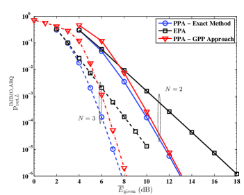
(a) IMIMO with ARQ

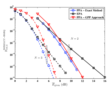
(b) IMIMO with CC-HARQ

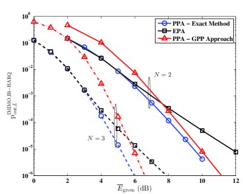
(c) IMIMO with IR-HARQ

Figure 2: Performance comparison of the proposed power allocation with the equal power allocation for an IMIMO system employing ARQ, CC-HARQ and IR-HARQ. The parameters for the simulation are $L=2,M=2$ and $R=2$ bps/Hz.

Proposed Power Allocation vs Equal Power Allocation: Figure 2 shows a performance comparison of PPA and EPA for IMIMO employing ARQ, CC-HARQ and IR-HARQ under different system parameter values. We plotted $\mathrm{p}_{\mathrm{out,}l}^{\mathrm{IMIMO,ARQ/HARQ\,type}}$ as a function of $\overline{E}_{\mathrm{given}}$. Following observations can be made from Figs. 2(a)-2(c). First, for higher values of outage probability, the EPA has a similar performance as that of the ‘PPA-exact method’, especially when the diversity order is high. The gains offered by the ‘PPA-exact method’ over EPA are more significant for smaller values of rate-outage probability (equivalently for higher average energy limit). Second, for the case of $L=N=2$, at a rate-outage probability of $10^{-5}$, the gain for the ‘PPA-exact method’ over the the EPA solution is 4 dB, 3.1 dB and 2.3 dB, for IMIMO with ARQ, CC-HARQ and IR-HARQ, respectively. However, the gains reduce as the diversity order of the system increases (i.e., as the value of $N$ increases). Third, in general, the closed-form ‘PPA-GPP approach’ provides higher outage probability than the ‘PPA-exact method’ and the performance gap between the two proposed schemes get closer as the energy limit $\overline{E}_{\mathrm{given}}$ increases, especially for smaller values of $L$ and $N$. The reason for the “loss” seen by the ‘PPA-GPP approach’ relative to the EPA for higher values of rate-outage probability is as follows. The approximation error of outage probability expressions is non-negligible for smaller values of $\overline{E}_{\mathrm{given}}$. The approximations become tighter (asymptotically equivalent) and the performance of the ‘GPP approach’ matches that of the exact method as $\overline{E}_{\mathrm{given}}$ value increases. To reduce the loss of the ‘PPA-GPP approach’ relative to ‘PPA-exact method’, one method is to use tighter approximations by considering the higher-order terms of the rate-outage probability expressions. However, when higher-order terms are also considered, they may include both positive and negative terms in the approximations, and this may restrict the use of the geometric programming approach to find a solution.

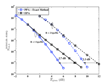
Figure 3: Performance comparison of PPA-exact method and EPA for IMIMO system employing IR-HARQ with different values of spectral efficiency, and $M=L=N=2$.

Comparison for Different Values of $R$: For an IMIMO system employing ARQ and CC-HARQ, we have the following proposition.

Proposition 1.

In an IMIMO system employing ARQ and CC-HARQ, for a given maximum number of transmissions $L$ and target rate-outage probability value of $\rho$, if $\left(P_{1,R_{1}},P_{2,R_{1}},\cdots,P_{L,R_{1}}\right)$ is the optimal power allocation solution with the average energy $E_{\mathrm{avg},1}$ for a spectral efficiency $R_{1}>0$ , then the optimal power allocation solutions and the average energy for a spectral efficiency of $R_{2}\neq R_{1}$ are given by

$$P_{l,R_{2}} =P_{l,R_{1}}\left(\frac{2^{R_{2}}-1}{2^{R_{1}}-1}\right),1\leq l\leq L,$$ (16)

$$E_{\mathrm{avg},2} =E_{\mathrm{avg},1}\left(\frac{2^{R_{2}}-1}{2^{R_{1}}-1}\right)$$

Proof:

The proof follows the same arguments as in the proof of Proposition 1 in [15]. ∎

Hence, for an IMIMO system employing ARQ and CC-HARQ, it is sufficient to solve the optimization problem in (6) for a single value of $R$ and scale the resulting power values according to (16) to obtain the optimal power values for a different value of $R$. In fact, a similar result as in Proposition 1 applies to EPA and GPP approaches as well. Hence for a given change in the value of $R$, the performance of all power allocation methods shift by the same amount and hence the relative performance difference remains the same independent of the value of $R$. However, for an IMIMO system with IR-HARQ, optimal power values for different values of $R$ does not scale according to (16), and hence performance difference between ‘PPA-exact method’ and EPA is different for different values of $R$, this can be seen from Fig. 3.

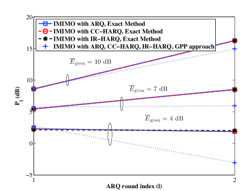
(a) $L=2,M=2,N=2,R=2\,\mbox{bpcu}$.

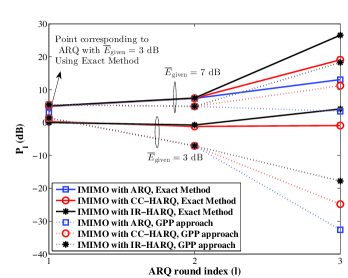
(b) $L=3,M=3,N=2,R=2\,\mbox{bpcu}$.

Figure 4: Comparison of $P_{l},1\leq l\leq L$ values to be used in different ARQ rounds for the three IMIMO schemes for a given $\overline{E}_{\mathrm{given}}$.

Power Values: Figure 4 shows the power values obtained by solving the optimization problems using different approaches. As can be seen from Fig. 4(a), for a given value of $\overline{E}_{\mathrm{given}}$, and for $L=2$, the three IMIMO systems have similar optimal power values obtained using the exact method, and the same power values obtained using the GPP approach. The reason for this can be explained by noting that, all the three optimization problems have the same average energy constraint as $\mathrm{p}_{\mathrm{out},1}^{\mathrm{IMIMO,ARQ/HARQ\,type}}$ is the same for all the three IMIMO systems (both the exact and approximated value). The approximated expression for packet drop probability $\mathrm{p}_{\mathrm{out},2}^{\mathrm{IMIMO,ARQ/HARQ\,type}}\propto 1/\left(P_{1}^{2}P_{2}^{2}\right)$ for all the three IMIMO systems, and hence they have the same solution using the GPP approach and similar optimal power values using the exact method. For $L=3$ in Fig. 4(b), we can clearly see the difference in the values of $P_{l}$ for the three IMIMO schemes using the exact method. Furthermore, as the value of $\overline{E}_{\mathrm{given}}$ increases, more power is allocated for “later ARQ rounds”, which are towards the end of the ARQ process. Since the objective of the optimization is to minimize the outage after $L$ ARQ rounds, we need to improve the probability of successful decoding during these later ARQ rounds. In other words, the energy cost associated with an unsuccessful decoding during these later ARQ rounds increases. Hence, for large values of $\overline{E}_{\mathrm{given}}$, PPA assigns high power values to these later ARQ rounds. We can also note from Fig. 4(b) that for smaller values of $\overline{E}_{\mathrm{given}}$, in case of IMIMO with ARQ, it is optimal to use the total transmission power during the first transmission attempt.

Practical Aspects: For limited real-time computational resources, one can solve the optimization problems offline by using nonlinear optimization techniques and store the results in a lookup table. For real-time online power allocation, using nonlinear optimization techniques to solve (6) may be too costly. In such cases, to achieve low target rate-outage probability, the simple closed-form ‘PPA-GPP approach’ is more computationally efficient and can provide closer performance to the ‘PPA-exact method’. If high outage probability (e.g., around $10^{-3}$ or higher) is acceptable, then one can use the EPA method.

VI Conclusions

We considered the problem of energy-efficient adaptive power allocation in IMIMO systems. In general, these optimization are difficult to solve as the rate-outage probability expressions are not mathematically tractable. We developed methods to convert the rate-outage probability expressions into a tractable form and solved the optimization problems using interior-point algorithms. We used asymptotically equivalent expressions of rate-outage probability and presented an unified geometric programming formulation for which the closed-form solution is derived. Possible extensions to the current work include, i) considering IMIMO systems with a subset of antennas transmitting (as in generalized spatial modulation) in each ARQ round instead of a single transmit antenna; ii) solving the optimization problems with the objective of minimizing the average delay or maximizing the long-term average throughput.

Appendix A Proof of $q_{i}\left(t\right),2\leq i\leq l$

Define $Q_{i}\left(s\right)$ as in [4]:

$$Q_{i}\left(s\right) =\frac{U\left(N,N+s,\frac{1}{P_{i}}\right)}{P_{i}^{N}}$$

$$=\int_{0}^{\infty}\frac{r^{N-1}\left(r+1\right)^{s-1}e^{-\frac{r}{P_{i}}}}{P_{i}^{N}\Gamma\left(N\right)}dr,i=2,\cdots,l$$ (17)

where $U\left(a,b,c\right)$ is the Tricomi confluent hypergeometric function [23], and $q_{i}\left(t\right),i=2,\cdots,l$ can be obtained as:

$$q_{i}\left(t\right) =\!L^{-1}\left(Q_{i}\left(s\right)\right)$$

$$=\int_{0}^{\infty}\!\underbrace{\left[\!\frac{1}{2\pi j}\int_{c-j\infty}^{c+j\infty}\!e^{st}\left(r+1\right)^{s-1}ds\!\right]}_{=\mathcal{L}^{-1}\left(\left(r+1\right)^{s-1}\right)}\!\frac{r^{N-1}e^{-\frac{r}{P_{i}}}}{P_{i}^{N}\Gamma\left(N\right)}dr\!$$

$$=\!\frac{e^{t}\!\left(e^{-t}-1\right)^{N-1}e^{\frac{1-e^{-t}}{P_{i}}}}{P_{i}^{N}\Gamma\left(N\right)}u\left(\!-t\right)$$ (18)

In (18), we used the relation $\mathcal{L}^{-1}\left(\left(r+1\right)^{s-1}\right)=\frac{1}{r+1}\mathcal{L}^{-1}\left(\left(r+1\right)^{s}\right)=\frac{1}{r+1}\mathcal{L}^{-1}\left(e^{s\ln\left(r+1\right)}\right)=\frac{1}{r+1}\delta\left(t+\ln\left(r+1\right)\right)$ and $\delta\left(.\right)$ is the Dirac delta function.

Appendix B Proof of Theorem 1

We write the Lagrangian function of (14) as:

$$\mathscr{L}\left(P_{1},\cdots,P_{L},\lambda,\mu_{1},\cdots,\mu_{L}\right) =\frac{W_{L}}{\left(P_{1}^{N}\cdots P_{L}^{N}\right)}\!+$$

$$\!\!\!\!\!\!\!\!\!\!\!\!\!\!\!\!\!\!\!\!\!\!\!\!\!\!\!\!\!\!\!\!\!\!\!\!\!\!\!\!\!\!\!\!\!\!\!\!\!\!\!\!\!\!\!\!\!\!\!\!\!\!\!\!\!\!\!\!\!\!\lambda\!\left(\!P_{1}\!+\!\sum_{l=2}^{L}\!P_{l}\frac{W_{l-1}}{\left(P_{1}^{N}\cdots P_{l-1}^{N}\right)}\!-\!\overline{E}_{\mathrm{given}}\!\right)-\sum_{l=1}^{L}\mu_{l}P_{l}$$ (19)

where $\lambda,\mu_{1},\cdots,\mu_{L}$ are the Lagrangian coefficients. Since the Karush-Khun-Tucker (KKT) conditions are necessary for an optimal solution, we have:

$$\!\!\!\!\!\!\!\!\!\!\!\!\!\!\!\!\!\!\!\!\!\!\!\!\!\!\!\!\!\!\left.\frac{\partial\mathscr{L}}{\partial P_{l}}\right|_{\left(P_{1}^{*},\cdots,P_{L}^{*},\lambda^{*},\mu_{1}^{*},\cdots,\mu_{L}^{*}\right)}=0,\mbox{ for }1\leq l\leq L$$ (20a)

$$\lambda^{*}\!\left(P_{1}^{*}\!+\!\sum_{l=2}^{L}\!P_{l}^{*}\!\frac{W_{l-1}}{\left(P_{1}^{*}\cdots P_{l-1}^{*}\right)^{N}}-\overline{E}_{\mathrm{given}}\right)=0$$ (20b)

$$\mu_{l}^{*}P_{l}^{*}=0,\mbox{ for }1\leq l\leq L$$ (20c)

Since the objective is to minimize $W_{L}/\left(P_{1}^{N}\cdots P_{L}^{N}\right)$, from (20c), it is clear that $\mu_{l}^{*}=0,\mbox{ for }1\leq l\leq L$. Considering (20a) for $l=L$ and simplifying, we have $\lambda^{*}=NW_{L}/\left(W_{L-1}\left(P_{L}^{*}\right)^{N+1}\right)$. Now considering (20a) $\mbox{for }1\leq l\leq L-1$, together with $\lambda^{*}$, we obtain

$$\left(P_{l}^{*}\right)^{N+1} =\frac{1}{W_{l-1}\prod_{m=l+1}^{L}\!\left(\!P_{m}^{*}\right)^{N}}\left(\!\vphantom{\left[\prod_{m=k+1}^{L}\left(P_{m}^{*}\right)^{N}\right]}\left(N+1\right)W_{L-1}\left(\!P_{L}^{*}\!\right)^{N+1}\!+\!\right.$$

$$\left.N\sum_{k=l}^{L-2}W_{k}P_{k+1}^{*}\left[\prod_{m=k+1}^{L}\left(P_{m}^{*}\right)^{N}\right]\right).$$ (21)

Substituting for $\left(P_{l+1}^{*}\right)^{N+1}$ in (21) and simplifying, we obtain the recursive relation for $2\leq l\leq L$ as:

$$P_{l}^{*}=\frac{W_{l-2}}{\left(1+N\right)W_{l-1}}\left(P_{l-1}^{*}\right)^{N+1},$$ (22)

Now to solve for $P_{1}^{*}$, we use the fact that the average energy constraint should be satisfied with equality at the optimal solution, i.e.,

$$P_{1}^{*}+\frac{W_{1}P_{2}^{*}}{\left(P_{1}^{*}\right)^{N}}+\frac{W_{2}P_{3}^{*}}{\left(P_{1}^{*}P_{2}^{*}\right)^{N}}+\frac{W_{L-1}P_{L}^{*}}{\left(P_{1}^{*}\cdots P_{L-1}^{*}\right)^{N}}=\overline{E}_{\mathrm{given}},$$ (23)

Now using (22) recursively in (23) with $W_{0}=1$, we obtain the solution for $P_{1}^{*}$ as in (15).

References

- [1] A. Mohammadi and F. Ghannouchi, “Single RF front-end MIMO transceivers,” IEEE Commun. Mag., vol. 49, no. 12, pp. 104–109, Dec. 2011.
- [2] R. Mesleh et al., “Spatial modulation,” IEEE Trans. Veh. Technol., vol. 57, no. 4, pp. 2228–2241, July 2008.
- [3] A. Stavridis et al., “Energy evaluation of spatial modulation at a multi-antenna base station,” in the Proc. of IEEE VTC, 2013.
- [4] P. Hesami and J. N. Laneman, “Incremental use of multiple transmitters for low-complexity diversity transmission in wireless systems,” IEEE Trans. Commun., vol. 60, no. 9, pp. 2522–2533, Sep. 2012.
- [5] P. Hesami and J. N. Laneman, “Low-complexity incremental use of multiple transmitters in wireless communication systems”, Proc. of Allerton, pp. 1613–1618, 2011.
- [6] H. El Gamal, G. Caire, and M. O. Damen, “The MIMO ARQ channel: diversity-multiplexing-delay tradeoff,” IEEE Trans. Inf. Theory, vol. 52, no. 8, pp. 3601–3621, Aug. 2006.
- [7] K. Nguyen, L. Rasmussen, A. Guillen i Fabregas, and N. Letzepis, “MIMO ARQ with multibit feedback: outage analysis,” IEEE Trans. Inf. Theory, vol. 58, no. 2, pp. 765–779, Feb. 2012.
- [8] H. Sun, J. H. Manton, and Z. Ding, “Progressive linear precoder optimization for MIMO packet retransmissions,” IEEE J. on Sel. Areas in Commun., vol. 24, no. 3, pp. 448–456, 2006.
- [9] B. Makki and T. Eriksson, “ On the performance of MIMO-ARQ systems with channel state information at the receiver,” IEEE Trans. Commun., vol. 62, no.5, pp. 1588-1603, May 2013.
- [10] P. Wu and N. Jindal, “Performance of hybrid-ARQ in block-fading channels: a fixed outage probability analysis,” IEEE Trans. Commun., vol. 58, no.4, pp. 1129-1141, Apr. 2010.
- [11] C. Shen, T. Liu, and M. P. Fitz, “On the average rate performance of hybrid-ARQ in quasi-static fading channels,” IEEE Trans. Commun., vol. 57, no. 11, pp. 3339–3352, Nov. 2009.
- [12] B. Makki, A. Graell I Amat, and T. Eriksson, “Green communication via power-optimized HARQ protocols,” IEEE Trans. veh. Tech., vol. 63, no. 1, pp. 161–177, Jan 2014.
- [13] L. Szczecinski, S. R. Khosravirad, P. Duhamel, and M. Rahman, “Rate allocation and adaptation for incremental redundancy truncated HARQ,” IEEE Trans. Commun., vol. 61, no. 6, pp. 2580–2590, Jun. 2013.
- [14] T. V. K. Chaitanya and E. G. Larsson, “Outage-optimal power allocation for hybrid ARQ with incremental redundancy,” IEEE Trans. Wireless Commun., vol. 10, no. 7, pp. 2069–2074, July 2011.
- [15] ——, "Optimal power allocation for hybrid ARQ with Chase combining in i.i.d. Rayleigh fading channels,” IEEE Trans. Commun., vol. 61, no. 5, pp. 1835–1846, May 2013.
- [16] ——, “Adaptive power allocation for HARQ with Chase combining in correlated Rayleigh fading channels,” IEEE WIreless Commun. Letters, vol. 3, no. 2, pp. 169-172, Apr. 2014.
- [17] G. Caire and D. Tuninetti, “The throughput of hybrid-ARQ protocols for the Gaussian collision channel,” IEEE Trans. Inform. Theory, vol. 47, no. 5, pp.1971–1988, July 2001.
- [18] G. P. Efthymoglou et al., “Performance analysis of coherent DS-CDMA systems in a Nakagami fading channel with arbitrary parameters,” IEEE Trans. Veh. Tech., vol. 46, no. 2, pp. 289–297, May 1997.
- [19] V. A. Aalo, T. Piboongungon, and G. P. Efthymoglou, “Another look at the performance of MRC schemes in Nakagami-m fading channels with arbitrary parameters,” IEEE Trans. Commun., vol. 53, no. 12, pp. 2002-2005, Dec. 2005.
- [20] S. Kalyani and R. M. Karthik, “The asymptotic distribution of maxima of independent and identically distributed sums of correlated or non-identical gamma random variables and its applications,” IEEE Trans. Commun., vol. 60, no. 9, pp. 2747–2758, Sep. 2012.
- [21] H. Exton, Multiple Hypergeometric Functions and Applications. Ellis Horwood, 1976.
- [22] M. Abramowitz and I. A. Stegun, Handbook of Mathematical Functions with Formulas, Graphs, and Mathematical Tables, 10th ed. U.S. Department of Commerce - N.B.S., Dec. 1972.
- [23] I. S. Gradshteyn and I. M. Ryzhik, Table of Integrals, Series, and Products, 7th edition. Academic Press, 2007.
- [24] A. Larmo et al., “The LTE link-layer design,” IEEE Commun. Mag., vol. 47, no. 4, pp. 52–59, Apr. 2009.
- [25] R. A. Waltz, J. L. Morales, J. Nocedal, and D. Orban, “An interior algorithm for nonlinear optimization that combines line search and trust region steps,” Mathematical Programming, vol. 107, no. 3, pp. 391–408, 2006.
- [26] L. F. Shampine, “Vectorized adaptive quadrature in Matlab,” J. of Comp. and App. Mathematics, vol. 211, no. 2. pp. 131–140, 2008.
- [27]