Accelerated materials property predictions and design using motif-based fingerprints
Abstract
Data-driven approaches are particularly useful for computational materials discovery and design as they can be used for rapidly screening over a very large number of materials, thus suggesting lead candidates for further in-depth investigations. A central challenge of such approaches is to develop a numerical representation, often referred to as a fingerprint, of the materials. Inspired by recent developments in chem-informatics, we propose a class of hierarchical motif-based topological fingerprints for materials composed of elements such as C, O, H, N, F, etc., whose coordination preferences are well understood. We show that these fingerprints, when representing either molecules or crystals, may be effectively mapped onto a variety of properties using a similarity-based learning model and hence can be used to predict relevant properties of a material, given that its fingerprint can be defined. Two simple procedures are introduced to demonstrate that the learning model can be inverted to identify the desired fingerprints and then, to reconstruct molecules which possess a set of targeted properties.
pacs:
71.15.Mb, 81.05.-t, 71.15.DxI Introduction
Data-driven approaches towards materials design and discovery are rapidly increasing in popularity, demand and potency. Hautier_review ; Curtarolo:nature ; Vinit_Nature ; Rampi:MLbook ; hastie:MLbook ; Curt:QSPR1 ; Curt:QSPR2 ; Tu:QSPR ; Curtarolo:03 ; Rajan200538 ; schon:ZAAC ; Meredig:14 ; Hansen:13 ; GuhaBook ; Varnek This emerging trend is fueled by the availability and emergence of large materials databases,MaterialsProject ; Bergerhoff:database ; Grazulis2012 as well as our ability to progressively accumulate materials data via high-throughput computations Ramakrishnan:SD ; Pilania_SR and experiments.MaterialsProject ; Bergerhoff:database ; Grazulis2012 Data-driven strategies aimed at rapid property predictions, and ultimately to rational or informed materials design, rely on exploiting the information content of past data, and using such information within heuristic or statistical interpolative learning models to provide estimates of properties of a new material. This approach is entirely analogous to similar pursuits undertaken within chem- and bio-informatics wherein lead candidates worthy of further in-depth investigations are identified rapidly in a first-level of screening.Rampi:MLbook ; hastie:MLbook ; GuhaBook
Data-driven property prediction strategies have two steps. The first involves representing materials numerically via descriptors, attribute vectors, or fingerprints. In the second step, using available “training” data sets, a mapping is established between the numerical representation of materials and their properties, thus leading to a prediction model. Subsequently, the properties of a new material are estimated using this model after reducing the material to its numerical representation.
One of the central challenges in this whole process is deciding on an appropriate and acceptable numerical representation of materials. The specific choice of this representation is entirely application dependent, and can range from high level descriptors (e.g., -band center, atomic electronegativities) Andriotis:14 ; ChiDam to topological features (e.g., substructural motifs) Brown:96 ; Brown:97 ; Pilania_SR to microscopic fingerprints that may capture chemical and configurational degrees of freedom (e.g., coulomb matrix, symmetry functions).CoulombMatrix ; Hansen:14 ; Lilienfeld:RDF ; Venke:14 Regardless of the specific choice, the representations are expected to satisfy certain basic requirements. These include invariance of the representation with respect to transformations of the material such as translation, rotation, and permutation of like elements. Moreover, it is desired that the representation be intuitive, elegant and physically and chemically meaningful.
In this contribution, inspired by developments in chem-informatics,GuhaBook ; Varnek we propose a class of hierarchical motif-based topological fingerprints. This choice, in which the motifs are molecular fragments of varying sizes, is particularly suited to representing molecules and solids composed of elements such as H, C, N, O, F, etc., whose coordination preferences are well understood. Large datasets of molecules and solids are considered, and it is shown that the fingerprints may be effectively mapped to a variety of properties using a similarity based learning algorithm. Moreover, it is demonstrated that the learning model may be inverted to identify fingerprints, and subsequently, to reconstruct actual molecules that possess a desired set of target properties.
II Datasets
In the present work, we restrict ourselves to systems composed of C, O and H. We used two datasets, one for molecules and one for crystals, to demonstrate the applicability of the proposed fingerprints. Of these two datasets, the former was taken from Ref. Ramakrishnan:SD, while the latter was prepared by us.
II.1 Molecule dataset
A dataset of more than 134,000 small molecules made up of C, O, H, N, and F was reported in Ref. Ramakrishnan:SD, . This reliable dataset, which contains the optimized geometries, and energetic, electronic, and thermodynamic properties calculated using the B3LYP hybrid exchange-correlation (XC) functional and the 6-31G(2df,p) basis set with the Gaussian 09 software, sets up the stage for many interesting data-mining works.Lilienfeld:delta ; Lilienfeld:molec A subset of this dataset, containing 45,708 molecules composed of C, O, and H was used in this work. Five properties were considered, including the atomization energy , the energy gap between highest occupied and lowest unoccupied molecular orbitals (HOMO-LUMO gap), the isotropic polarizability , the heat capacity , and the zero-point vibration energy .
II.2 Crystal dataset
In addition to the molecules dataset, we prepared another dataset of 215 organic crystals comprising of C, O, and H. This includes
-
1.
12 existing polymers composed of C, O, and H,
-
2.
16 new polymer structures predicted by the minima-hopping methodMHM:OrganovBookChapter ; Goedecker:MHM ; Amsler:MHM and USPEXUSPEX for 16 quasi-one-dimensional polymer chain models reported in Ref. Vinit_Nature, ,
-
3.
34 organic crystals composed of C and H and 153 organic crystals composed of C, O, and H obtained from Crystallography Open Database. Grazulis2012
The obtained structures were optimized by first-principles calculations within the DFT formalism as implemented in Vienna Ab initio Simulation Package (vasp), vasp1 ; vasp2 ; vasp3 ; vasp4 utilizing the semi-local rPW86 XC functional MurrayrPW86 and a plane wave energy cutoff of 400 eV. A Monkhorst-Pack k-point meshmonkhorst with the spacing of no more than Å-1 in the reciprocal space were used for sampling the Brillouin zone, while the van der Waals interactions were estimated with the non-local density functional vdW-DF2. vdW-DF2 Convergence was assumed when the atomic forces exerting on the atomic sites are smaller than 0.01 eV/Å. The entire crystals dataset, which includes the optimized structures, the atomization energies , the band gaps , and the electronic and ionic parts of the dielectric constants, and , can be found in the Supplemental Material. supplement
III Fingerprints
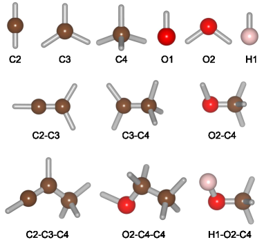
A hierarchy of equilibrium structure fingerprints of the same family with increasing levels of sophistication are proposed here. The construction of fingerprints was guided by two simple chemical concepts, i.e., chemical bonds and coordination number. The former intuitively characterizes the short-range interatomic interactions Pauling while the latter is the number of bonds involving a given atom. In major classes of materials composed of light elements like C, H, O, N, and F, these concepts are well-defined. In particular, the length of a given bond involving these elements falls in a narrow range (see Refs. Allen:Table, ; AllenBook, for a comprehensive bond length statistics). For instance, the equilibrium length of a single bond between two C atoms is Å, the length of a double bond between two C atoms is Å, and the length of a double bond between a C atom and an O atom is Å.Allen:Table ; AllenBook The coordination number is also well-defined, i.e., for a C atom, it can only be 2, 3, or 4 while each O atom can generally bond with 1 or 2 other atoms. Therefore, atoms in a structure can be unambiguously classified (or labeled) by where is the type of the element () and is its coordination number. Likewise, bonds can be specified by the types of its two ends, e.g., . For the datasets of C, O, and H, the six possible atom types are C2, C3, C4, O1, O2, and H1 while there are sixteen chemically permissible types of bonds, namely C2-C2, C2-C3, C2-C4, C2-O1, C2-O2, C2-H1, C3-C3, C3-C4, C3-O1, C3-O2, C3-H1, C4-C4, C4-O2, C4-H1, O2-O2, and O2-H1. Except C2-O1, C2-O2, and O2-O2, thirteen of them are present in our molecules and crystals datasets. The atom and bond types belong to a family of related structural building units (subsequently described) that can be used to numerically represent the materials structures and hence, are used to define the fingerprints. In particular, the order fingerprint is defined in terms of its components as
| (1) |
Here, is the number of building units (or fragments or motifs) of type and is the number of atoms either in the molecule or in the unit cell of a crystal. Four types of fingerprints, namely , , , and , are discussed in the following subsections.
III.1 -order fingerprint,
The simplest (-order) fingerprint represents the fractions of all the element types existing in the structures, i.e., . Therefore, in the definition (1) of , is the number of atoms of element . This fingerprint is a three-dimensional vector whose components satisfy a simple normalization condition .
III.2 -order fingerprint,
Next in the hierarchy is the case in which is the number of atoms which are fold coordinated. is a 6-dimensional vector, satisfying several constraints established from the definition or from the chemistry. The first one is the normalization condition, given as
| (2) |
Within the two datasets, all the C2 atoms should be grouped by pairs, forming triple bonds. Therefore, the number of C2 atoms, which is , must be an even integer. Moreover, since each C3 atom only make a double bond with either an O1 atom or another C3 atom, one must have while is an even number. By examining the connectivity of a structure, another constraint reads
| (3) |
where is the number of closed loops of bonds and is a structure-dependent parameter. For molecules and crystals composed of isolated substructures (or molecules), while for crystals composed of connected substructures, . The derivation of this constraint is given in Appendix A. The last constraint of is written in the form of a recursion relation, i.e.,
| (4) |
III.3 -order fingerprint,
Both and are local, representing the density of the atom types of a material. The equilibrium interatomic distance is somehow captured by the -order fingerprint where all the possible bonds are counted. is a 13-dimensional vector whose components, , represent the normalized number of the bonds in the structure. From , can readily be determined by a recursion relation
| (5) |
where is used to remove the double counting when [see Appendix B for the derivation of (5)]. Through this recursion relation, all the constraints that obeys are applicable for . We note that was discussed in several previous works, e.g., in Refs. bond_energy, ; CoulombMatrix, ; Moussa:2012, under the name of “bond counting”. This fingerprint can also be regarded as a generalization of “doubles”, the fingerprint defined in Ref. Pilania_SR, for the chain models of polymers.
III.4 -order fingerprint,
In the -order fingerprint , the number of two-bond catenation is represented, i.e., . In particular, the definition (1) for involves , which is the number of sequences, or equivalently, the catenation of two bonds and . Considering compounds of C, O, and H, there are 125 possible distinct catenation of two bonds and . From , can be determined as (see Appendix B)
| (6) |
Similar to , can be viewed as a generalization of “triples”, the fingerprint examined in Ref. Pilania_SR, .
IV Property prediction model
A learning model is critical in order to map the fingerprints to properties. In this work, we chose Gaussian kernel ridge regression (KRR),hofmann2008 ; Muller:KRR ; hastie:MLbook the technique which has successfully been used in material properties predictions CoulombMatrix ; Pilania_SR ; Venke:14 ; Lilienfeld:delta ; Lilienfeld:molec Within this model, the input fingerprints are transformed into higher-dimensional space whereby a linear relation between the transformed fingerprints and the associated properties can be established. This mapping involves the distances between fingerprints and can be regarded as a similarity-based prediction model, i.e., similar properties may be predicted for materials with similar fingerprints.
In the KRR model, the property of a structure is predicted as an weighted sum of Gaussians
| (7) |
where runs over all the fingerprints in the training dataset. Here, is the distance between fingerprints and , defined as the Euclidean metric . The Gaussian width parameter and the regression coefficients are determined within the training phase whence a regularized objective function is minimized.hofmann2008 ; Muller:KRR ; hastie:MLbook During this phase, and the regularization parameter are determined by -fold cross validation on the training set ( in this work). Within this method, the training dataset is split into bins, any of the bins is considered to be a new test dataset while the remaining bins form a new training datatest. This procedure is repeated for each of the bins and for every value of and on a preselected logarithmic-scale grid. The optimal values of and , i.e., those leading to the minimum -fold cross-validation (mean absolute) error, are used to compute of the entire dataset.
V Property prediction results
V.1 Molecules dataset
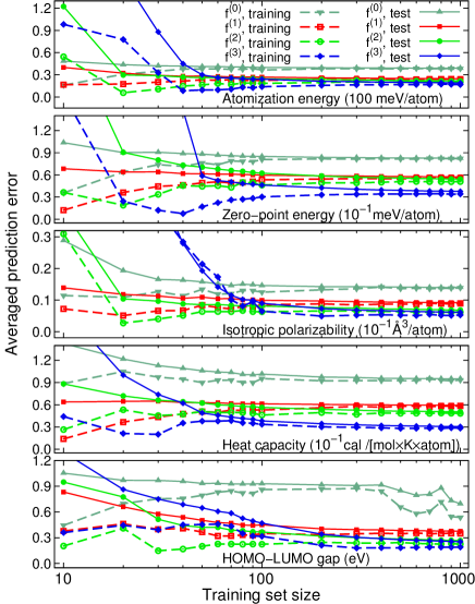
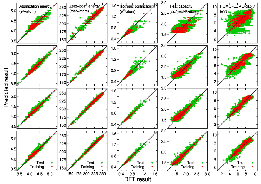
The four fingerprints considered, namely , , , and , were used to represent the molecules dataset. To mimic the learning and prediction processes, the dataset was randomly partitioned into a training dataset and a test dataset. The KRR model was then trained on the training dataset using five-fold cross validation before predictions were made on the test dataset. We show in Fig. 2 the learning curves of , , , , and , plotting the training and test errors against the number of molecules in the training dataset (data reported in this figure was averaged over 30 independent runs). In addition, predictions for the test dataset of 44,708 molecules after training the KRR model on a dataset of 1,000 molecules are shown in Fig. 3. As discussed in detail below, both Fig. 2 and Fig. 3 indicate that all of these properties can be very well predicted by using either or , provided that the KRR model is trained on a training dataset of or more data points.
The general tendency, as revealed by Fig. 2, is that higher-order fingerprints offer more accurate predictions. The -order fingerprint can be used to roughly estimate energy-related quantities, i.e., and while it can not be used for others. For instance, can not be predicted with because this fingerprint is totally local in nature, encoding no information at any finite range. Consequently, the finite conjugation length, known to signal the energy gap reduction in complex (conjugated) systems (see, for example Ref. StallingaBook, ), is not captured by . Fingerprints of higher orders, e.g., , and , contain some information at increasing ranges, allowing for systematically better predicting . These fingerprints also work sufficiently well in predicting and . With , the averaged error in predicting is meV/atom while this error is reduced to meV/atom and meV/atom if and , respectively, are used. The very good power of in predicting reproduces the similar conclusions drawn for the “bond counting” fingerprint by Ref. Moussa:2012, . This behavior is understandable because the dissociation energy of chemical bonds in organic molecules and crystals, which dominates the stability of these systems, are well-defined bond_energy in the same fashion with the bond length as previously discussed. Interestingly, this predictive power can significantly be improved if more advanced fingerprints, i.e., those can capture the small perturbations of interatomic distances like Coulomb matrix, are used.Lilienfeld:delta ; Lilienfeld:molec Compared to and , is significantly better in predicting . The considerable improvement in the predictions of when is used instead of may indicate the key contribution from polar bonds to the high-value regime of .
V.2 Crystals dataset
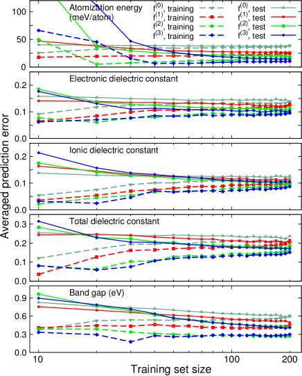
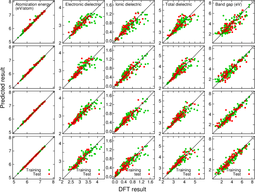
We performed similar predictions for the dataset of 215 crystals containing C, O, and H. Using the KRR model coupled with , , , and , five properties of these crystals, including the atomization energies , the band gap , the electronic dielectric constant , the ionic dielectric constant , and the total dielectric constant , were predicted. We show in Fig. 4 the learning curves, representing the errors of the predictions using these fingerprints, averaged over independent runs. In Fig. 5, the predictions for the five properties are given, using the KRR model trained on a random training set of data points.
Clearly, the tendency of the prediction performances on the crystals dataset is similar to those of the molecules dataset, i.e., high accuracies are obtained with fingerprints of higher orders, and properties which are governed by long-ranged information, e.g., band gap , can only be predicted with high-order fingerprints. For the atomization energy , predictions with and leads to quite high averaged errors, which reduced to meV/atom and meV/atom when and , respectively, were used. Overall, all the five examined properties can be predicted well when high-order fingerprints are used to represent the crystals. For instance, by employing , the averaged error in predicting is eV while the electronic dielectric constant and the ionic dielectric constant can be predicted with an averaged error of .
VI Utilities of the fingerprints
The demonstrated predictive power of the KRR model, which uses to represent materials structures, inspires the idea of using this model to rationally optimize materials for a targeted property , the concept often referred to as “inverse design”. Ceder ; Besenbacher20031998 ; FrancesNature ; QUA:QUA24687 In fact, a large number of success stories along this direction have been reported in the past, using various approaches, e.g., iteratively optimizing the properties of a given compound or on-the-fly screening when searching for stable structures. Lilienfeld:inverse ; Marcon:07 ; Lilienfeld:energy_gradient ; Lilienfeld:alchemi ; Wang:design_molec ; Keinan_design_molec ; Keinan_design_molec_2 ; Rinderspacher_design_molec ; Curtarolo2003 ; Greeley ; Avezac2012 ; XiangInvDesign ; Phillips:ML Here, our idea is that starting from a trained KRR model, fingerprints which correspond to the desired properties can be predicted. Then, molecular structures will be reconstructed from the predicted fingerprints. Finally, the targeted properties will be verified by DFT calculations at the same level with those used for the training dataset.
The greatest challenge of this procedure is to ensure that the predicted fingerprint is physically and chemically meaningful, i.e., at least one material structure can be reconstructed from it.Lilienfeld:CCS ; Lilienfeld:ensemble Therefore, one must mathematically define the subspace of the meaningful fingerprints, and then limit the search for desired fingerprints within this subspace. We present two approaches which can be used for designing molecules (the work of designing crystals is not considered here).
VI.1 Design via enumeration
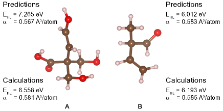
The central idea of this approach is that the components of a given fingerprint can be enumerated in a given way so that it is meaningful. We used for a demonstration because predictions using this fingerprint are good while its dimensionality is not too high like . We first implemented the applicable rules involving bonds and coordination numbers by defining five “backbone” blocks. They include C4, CC (a pair of C3 atoms with a double bond), CC (a pair of C2 atoms with a triple bond), CO (one C3 and one O1 atom linked by a double bond), and O2. By definition, all of the dangling bonds starting from these blocks are single, thus any of them can be connected to others without any constraint. Then, given a set of backbone blocks, all the possible arrangements can be scanned, keeping track of the connectivity to eliminate some dangling bonds, and saturating the remaining dangling bonds by either H1 or OH, referred to as “ending” blocks. From the obtained arrangements, can be unambiguously determined and their properties were predicted. Those with targeted properties were singled out to rebuild molecular structures for validating calculations. We show in Fig. 6 two optimized molecules constructed from two of the predicted fingerprints, labeled by A and B, accompanied by the predicted and calculated and . The results given in Fig. 6 indicate that the desired molecules are indeed obtained.
VI.2 Design via inversion
Different from the enumeration approach, this procedure aims to directly determine the fingerprints, starting from desired properties. This goal can be achieved by optimizing an objective function, aiming towards the desired properties while applying the constraints that ensure the fingerprints considered are meaningful. Because the reconstruction step requires a simple enough fingerprint, was selected for this approach. Among the constraints established for , (2) and (3) are explicitly imposed in the objective function defined below
| (8) |
Here, , and are the Lagrange multipliers associated with the constraints while is the property (or properties) of the trial fingerprint predicted by the trained KRR model. In practice, we evaluated by averaging many predictions, each of them was given by the KRR model trained on a randomly selected training dataset of 1,000 data points. All the terms in (8) are given in the quadratic form to smoothen . Generally, the problem of minimizing (performed with simulated annealingKirkpatrick13051983 in this work) returns many solutions . For each of them, was determined by minimizing another objective function defined as
| (9) |
where returns the closest integer to . Once is determined, a post-screening step is performed to consider the possibility of and to single out the fingerprints so that and are positive even numbers. Such fingerprints are meaningful, i.e., molecules can be built up from any of them.
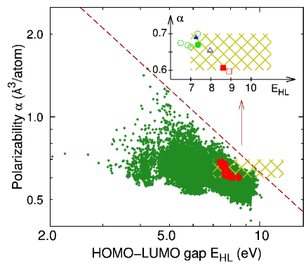
We demonstrate this procedure by optimizing two properties simultaneously, i.e., and . We note that these properties seem to be competing, as shown in Fig. 7 where an asymptotic limit of the form can be seen (similar limit between two related properties of crystals, namely and was documented earlier in Ref. Chenchen:polymer, ). An examination of Fig. 3 reveals that the prediction of using is fairly good in the region of Å3/atom. For this reason, we searched for new molecules, i.e., those that do not exist in the molecules dataset, of which Å3/atom while eV and show the results in Fig. 7. While the calculated of the molecules dataset can reach the upper limit of eV, all the predictions for by the KRR model are below 9 eV. The reason is given in Fig. 3 which clearly implies that when is coupled with the KRR model, high values of ( eV) are generally underestimated by roughly 1 eV. Three of the predicted fingerprints, labeled by C, D, and E, were selected for rebuilding new molecules. From either C or E, only one molecule can be constructed while many different molecules correspond to D. All of the molecules reconstructed from C, D, and E were optimized and then their and were calculated with Gaussian 09,GAUSSIAN09 using the 6-31G(2df,p) basis set and the B3LYP XC functional.B3LYP1 ; B3LYP2 The results are summarized in Table 1 and in the inset of Fig. 7, demonstrating that the molecules with desired values of and were actually obtained. Detailed information on all of the designed molecules can be found in the Supplemental Material.supplement
VI.3 Remarks
It is worth noting that the key feature of which is useable for the described enumeration and inversion design procedures is their discontinuity with respect to slight configurational perturbations. Because all the possible chemical bonds appearing in a molecule comprising C, O, and H are well-defined, it is very likely that the optimization step performed on the reconstructed molecules preserves the predicted fingerprint. Moreover, the efficiency of the designing approaches depends on several factors, including the prediction accuracy of the fingerprints used. Although predictions by using high-order fingerprints are systematically better, the complexity generated by their high dimensionality is significant. Comparing to the procedure described above, that utilizing or needs roughly 10 and 100 more constraints for ensuring the considered fingerprints are meaningful. If the dimensionality of can considerably be reduced, it may then be used for the inversion approach.
VII Conclusions
To summarize, we have systematically studied a family of motif-based topological fingerprints which can numerically represent major classes of molecules and crystals. By using a similarity based learning algorithm, these fingerprints can be mapped onto various properties of molecules and crystals, significantly accelerating their properties prediction. A major advantage of these fingerprints is clearly demonstrated via two procedures for designing molecules, one by enumeration and the other by inversion. These procedures rely on the accelerated properties prediction to identify the desired fingerprints, and then to reconstruct molecules that possess one or more targeted properties. We note that although only molecules and crystals comprising C, O, and H are considered in this contribution, our results can straightforwardly be generalized to those containing other light elements whose coordination preferences are well established, e.g., N and F.
| Label | Predicted | Calculated | ||||
|---|---|---|---|---|---|---|
| C | 11 | |||||
| D | 18 | |||||
| E | 14 | |||||
Acknowledgements.
The authors thank Venkatesh Botu, Ghanshyam Pilania, and Vinit Sharma for useful discussions and O. Anatole von Lilienfeld for drawing our attention to some important relevant works. The present work was supported by a Multi-University Research Initiative (MURI) grant from the Office of Naval Research, under award number N00014100944. Part of the computational work was done with our sponsored TeraGrid XSEDE allocation.xsede_allocationAppendix A Constraint of derived from elementary chemical rules
Constraint (3) was derived with an assumption that the desired molecular structure is connected, i.e., any pair of atoms are connected by at least one sequence of the allowed chemical bonds. Let us take a molecule in which is the number of the blocks . Starting from the applicable chemical rules, all the two-fold coordinated carbon atoms are grouped by pairs, forming units of , each of which is a pair of carbon atoms linked by a triple bond. Next, one-fold coordinated oxygen atoms must bond with three-fold coordinated carbon atoms to form units of . Then, the remaining three-fold coordinated carbon atoms are grouped together by pairs, forming units of . Therefore, the set of the blocks now contains units of , , , and . Assuming that these units are isolated, the total number of dangling bonds starting from them is , or simply
| (10) |
By joining units together, the number of dangling bonds that will be annihilated to form inter-unit bonds is where is the number of loops of bonds, each of which costs extra 2 bonds. Therefore, the number of remaining dangling bonds is
| (11) |
All of these dangling bonds must be saturated by hydrogen atoms, thus
| (12) |
The constraint (3) can then be obtained when we divide Eq. (12) by . This constraint is applicable not only for molecules but also for crystals formed by repeatedly placing an isolated molecule in a periodic grid. If these molecules are not isolated, i.e., they form a network of dimensions, dangling bonds are used to form the network (assuming that the network are formed only by single bonds). Thus, Eq. 12 is given as
| (13) |
In the general case when not only single bonds involve the network formation, the parameter used in Eq. 13 is not necessarily an integer.
Appendix B Derivation of the recursion relations of and
B.1 Recursion relations of
The number of blocks can be determined by counting all the bonds of type. By summing all the number of bonds, the bonds are counted twice. Therefore
| (14) |
Then, the recursion relation of can be obtained by dividing (14) by the total number of atoms .
B.2 Recursion relations of
Similar to the derivation of (14), the fingerprint component can be determined by counting the number of sequences before dividing by . In such a procedure, the sequences are counted twice. Thus, after removing the double counting, we obtain
| (15) |
We note that one can also count the number of sequences before dividing the total number by . Thus
| (16) |
By dividing (15) and (16) by , two equivalent recursion relations are obtained. Moreover, we note that (15) and (16) set up a constraint that must also satisfy.
References
- (1) G. Hautier, A. Jain, and S. Ong, J. Mater. Sci. 47, 7317 (2012).
- (2) S. Curtarolo, G. L. W. Hart, M. B. Nardelli, N. Mingo, S. Sanvito, and O. Levy, Nat. Matter. 12, 191 (2013).
- (3) V. Sharma, C. C. Wang, R. G. Lorenzini, R. Ma, Q. Zhu, D. W. Sinkovits, G. Pilania, A. R. Oganov, S. Kumar, G. A. Sotzing, S. A. Boggs, and R. Ramprasad, Nat. Commun. 5, 4845 (2014).
- (4) T. Mueller, A. G. Kusne, and R. Ramprasad (unpublished).
- (5) T. Hastie, R. Tibshirani, and J. Friedman, The Elements of Statistical Learning: Data Mining, Inference, and Prediction, 2nd ed. (Springer-Verlag, New York, 2009).
- (6) C. M. Breneman and M. Rhem, J. Comput. Chem. 18, 182 (1997).
- (7) N. Sukumar, M. Krein, Q. Luo, and C. Breneman, J. Mater. Sci. 47, 7703, (2012).
- (8) T. Le, V. C. Epa, F. R. Burden, and D. A. Winkler, Chem. Rev. 112, 2889 (2012).
- (9) S. Curtarolo, D. Morgan, K. Persson, J. Rodgers, and G. Ceder, Phys. Rev. Lett. 91, 135503 (2003).
- (10) K. Rajan, Mater. Today 8, 38 (2005).
- (11) J. C. Schön, Z. Anorg. All. Chem. 640, 2717 (2014).
- (12) B. Meredig, A. Agrawal, S. Kirklin, J. E. Saal, J. W. Doak, A. Thompson, K. Zhang, A. Choudhary, and C. Wolverton, Phys. Rev. B 89, 094104 (2014).
- (13) K. Hansen, G. Montavon, F. Biegler, S. Fazli, M. Rupp, M. Scheffler, O. A. von Lilienfeld, A. Tkatchenko, and K.-R. Müller, J. Chem. Theor. Comput. 9, 3404 (2013).
- (14) R. Guha and A. Bender, Computational Approaches in Cheminformatics and Bioinformatics (John Willey & Sons, New York, 2011).
- (15) A. Varnek, in Chemoinformatics and Computational Chemical Biology, Vol. 672 of Methods in Molecular Biology, edited by J. Bajorath (Humana Press, New York, NY, 2011), pp. 213–243.
- (16) A. Jain, S. P. Ong, G. Hautier, W. Chen, W. D. Richards, S. Dacek, S. Cholia, D. Gunter, D. Skinner, G. Ceder, and K. A. Persson, APL Materials 1, 011002, (2013).
- (17) G. Bergerhoff, I. Brown, F. Allen, G. Bergerhoff, and R. Sievers, Crystallographic Databases (International Union of Crystallography, Chester, 1987).
- (18) S. Gražulis, A. Daškevič, A. Merkys, D. Chateigner, L. Lutterotti, M. Quirós, N. R. Serebryanaya, P. Moeck, R. T. Downs, and A. Le Bail, Nucleic Acids Res. 40, D420 (2012).
- (19) R. Ramakrishnan, P. O. Dral, M. Rupp, and O. A. von Lilienfeld, Sci. Data 1, 140022 (2014).
- (20) G. Pilania, C. Wang, X. Jiang, S. Rajasekaran, and R. Ramprasad, Sci. Rep. 3, 2810 (2013).
- (21) A. N. Andriotis, G. Mpourmpakis, S. Broderick, K. Rajan, S. Datta, M. Sunkara, and M. Menon, J. Chem. Phys. 140, 094705 (2014).
- (22) H. C. Dam, T. L. Pham, T. B. Ho, A. T. Nguyen, and V. C. Nguyen, J. Chem. Phys. 140, 044101 (2014).
- (23) R. D. Brown and Y. C. Martin, J. Chem. Inf. Comput. Sci. 36, 572 (1996).
- (24) R. D. Brown and Y. C. Martin, J. Chem. Inf. Comput. Sci. 37, 1 (1997).
- (25) M. Rupp, A. Tkatchenko, K.-R. Müller, and O. A. von Lilienfeld, Phys. Rev. Lett. 108, 058301 (2012).
- (26) K. Hansen, F. Biegler, O. A. von Lilienfeld, K.-R. Müller, and A. Tkatchenko (unpublished).
- (27) O. A. von Lilienfeld, R. Ramakrishnan, M. Rupp, and A. Knoll, Int. J. Quant. Chem. (2015), accepted.
- (28) V. Botu and R. Ramprasad, Int. J. Quant. Chem. (2015), DOI: 10.1002/qua.24836.
- (29) R. Ramakrishnan, P. O. Dral, M. Rupp, and O. A. von Lilienfeld, arXiv:1503.04987 (unpublished).
- (30) R. Ramakrishnan and O. A. von Lilienfeld, Chimia (2015), accepted.
- (31) S. Goedecker, in Modern Methods of Crystal Structure Prediction, edited by A. R. Oganov (Wiley-VCH, Weinheim, Germany, 2011), Chap. 7, pp. 147–180.
- (32) S. Goedecker, J. Chem. Phys. 120, 9911 (2004).
- (33) M. Amsler and S. Goedecker, J. Chem. Phys. 133, 224104 (2010).
- (34) C. W. Glass, A. R. Oganov, and N. Hansen, Comput. Phys. Commun. 175, 713 (2006).
- (35) G. Kresse and J. Hafner, Phys. Rev. B 47, 558 (1993).
- (36) G. Kresse, Ph.D. thesis, Technische Universität Wien, 1993.
- (37) G. Kresse and Furthmüller, J. Comput. Mater. Sci. 6, 15 (1996).
- (38) G. Kresse and J. Furthmüller, Phys. Rev. B 54, 11169 (1996).
- (39) E. D. Murray, K. Lee, and D. C. Langreth, J. Chem. Theor. Comput. 5, 2754 (2009).
- (40) H. J. Monkhorst and J. D. Pack, Phys. Rev. B 13, 5188 (1976).
- (41) K. Lee, É. D. Murray, L. Kong, B. I. Lundqvist, and D. C. Langreth, Phys. Rev. B 82, 081101(R) (2010).
- (42) See Supplemental Material for more information reported in this paper.
- (43) L. Pauling, J. Am. Chem. Soc. 54, 3570 (1932).
- (44) F. H. Allen, O. Kennard, D. G. Watson, L. Brammer, A. G. Orpen, and R. Taylor, J. Chem. Soc., Perkin Trans. II S1 (1987).
- (45) F. H. Allen, D. G. Watson, L. Brammer, A. G. Orpen, and R. Taylor, in International Tables for Crystallography, Mathematical, Physical and Chemical Tables, 3rd ed., edited by E. Prince (Kluwer Academic Publishers, Norwell, MA, USA, 2004), Chap. 9.5.
- (46) S. W. Benson, J. Chem. Educ. 42, 502 (1965).
- (47) J. Moussa, Phys. Rev. Lett. 109, 059801 (2012).
- (48) T. Hofmann, B. Sch lkopf, and A. J. Smola, Ann. Stat. 36, 1171 (2008).
- (49) K. Muller, S. Mika, G. Ratsch, K. Tsuda, and B. Scholkopf, IEEE Trans. Neural Netw. 12, 181 (2001).
- (50) P. Stallinga, Electrical characterization of organic electronic materials and devices (John Wiley & Sons, West Sussex, UK, 2009).
- (51) G. Ceder, Y. M. Chiang, D. R. Sadoway, M. K. Aydinol, Y. I. Jang, and B. Huang, Nature 392, 694 (1998).
- (52) F. Besenbacher, I. Chorkendorff, B. S. Clausen, B. Hammer, A. M. Molenbroek, J. K. N rskov, and I. Stensgaard, Science 279, 1913 (1998).
- (53) A. Franceschetti and A. Zunger, Nature 402, 60 (1999).
- (54) T. Weymuth and M. Reiher, Int. J. Quant. Chem. 114, 823 (2014).
- (55) O. A. von Lilienfeld, R. D. Lins, and U. Rothlisberger, Phys. Rev. Lett. 95, 153002 (2005).
- (56) V. Marcon, O. A. von Lilienfeld, and D. Andrienko, J. Chem. Phys. 127, 064305 (2007).
- (57) O. A. von Lilienfeld, J. Chem. Phys. 131, (2009).
- (58) D. Sheppard, G. Henkelman, and O. A. von Lilienfeld, J. Chem. Phys. 133, 084104 (2010).
- (59) M. Wang, X. Hu, D. N. Beratan, and W. Yang, J. Am. Chem. Soc. 128, 3228 (2006).
- (60) S. Keinan, X. Hu, D. N. Beratan, and W. Yang, J. Phys. Chem. A 111, 176 (2007).
- (61) S. Keinan, W. D. Paquette, J. J. Skoko, D. N. Beratan, W. Yang, S. Shinde, P. A. Johnston, J. S. Lazo, and P. Wipf, Org. Biomol. Chem. 6, 3256 (2008).
- (62) B. C. Rinderspacher, J. Andzelm, A. Rawlett, J. Dougherty, D. N. Beratan, and W. Yang, J. Chem. Theor. Comput. 5, 3321 (2009).
- (63) S. Curtarolo, D. Morgan, K. Persson, J. Rodgers, and G. Ceder, Phys. Rev. Lett. 91, 135503 (2003).
- (64) J. Greeley and M. Mavrikakis, Nat. Mater. 3, 810 (2004).
- (65) M. d’Avezac, J.-W. Luo, T. Chanier, and A. Zunger, Phys. Rev. Lett. 108, 027401 (2012).
- (66) H. J. Xiang, B. Huang, E. Kan, S.-H. Wei, and X. G. Gong, Phys. Rev. Lett. 110, 118702 (2013).
- (67) C. L. Phillips and G. A. Voth, Soft Matter 9, 8552 (2013).
- (68) O. A. von Lilienfeld, Int. J. Quant. Chem. 113, 1676 (2013).
- (69) O. A. von Lilienfeld and M. E. Tuckerman, J. Chem. Phys. 125, 154104 (2006).
- (70) S. Kirkpatrick, C. D. Gelatt, and M. P. Vecchi, Science 220, 671 (1983).
- (71) C. C. Wang, G. Pilania, S. A. Boggs, S. Kumar, C. Breneman, and R. Ramprasad, Polymer 55, 979 (2014).
- (72) M. J. Frisch, G. W. Trucks, H. B. Schlegel, G. E. Scuseria, M. A. Robb, J. R. Cheeseman, G. Scalmani, V. Barone, B. Mennucci, G. A. Petersson, H. Nakatsuji, M. Caricato, X. Li, H. P. Hratchian, A. F. Izmaylov, J. Bloino, G. Zheng, J. L. Sonnenberg, M. Hada, M. Ehara, K. Toyota, R. Fukuda, J. Hasegawa, T. Ishida, Nakajima, Y. Honda, O. Kitao, H. Nakai, T. Vreven, J. A. Montgomery, Jr., J. E. Peralta, F. Ogliaro, M. Bearpark, J. J. Heyd, E. Brothers, K. N. Kudin, V. N. Staroverov, R. Kobayashi, J. Normand, K. Raghavachari, A. Rendell, J. C. Burant, S. S. Iyengar, J. Tomasi, M. Cossi, N. Rega, J. M. Millam, M. Klene, J. E. Knox, J. B. Cross, V. Bakken, C. Adamo, J. Jaramillo, R. Gomperts, R. E. Stratmann, O. Yazyev, A. J. Austin, R. Cammi, C. Pomelli, J. W. Ochterski, R. L. Martin, K. Morokuma, V. G. Zakrzewski, G. A. Voth, P. Salvador, J. J. Dannenberg, S. Dapprich, A. D. Daniels, O. Farkas, J. B. Foresman, J. V. Ortiz, J. Cioslowski, and D. J. Fox, Gaussian 09, Revision A.02, Gaussian, Inc., Wallingford CT, 2009.
- (73) A. D. Becke, J. Chem. Phys. 98, 5648 (1993).
- (74) P. J. Stephens, F. J. Devlin, C. F. Chabalowski, and M. J. Frisch, J. Phys. Chem. 98, 11623 (1994).
- (75) J. Towns, T. Cockerill, M. Dahan, I. Foster, K. Gaither, A. Grimshaw, V. Hazlewood, S. Lathrop, D. Lifka, G. D. Peterson, R. Roskies, J. R. Scott, and N. Wilkins-Diehr, Comput. Sci. Eng. 16, 62 (2014).