Nonlinear time-series analysis revisited

Abstract

In 1980 and 1981, two pioneering papers laid the foundation for what became known as nonlinear time-series analysis: the analysis of observed data—typically univariate—via dynamical systems theory. Based on the concept of state-space reconstruction, this set of methods allows us to compute characteristic quantities such as Lyapunov exponents and fractal dimensions, to predict the future course of the time series, and even to reconstruct the equations of motion in some cases. In practice, however, there are a number of issues that restrict the power of this approach: whether the signal accurately and thoroughly samples the dynamics, for instance, and whether it contains noise. Moreover, the numerical algorithms that we use to instantiate these ideas are not perfect; they involve approximations, scale parameters, and finite-precision arithmetic, among other things. Even so, nonlinear time-series analysis has been used to great advantage on thousands of real and synthetic data sets from a wide variety of systems ranging from roulette wheels to lasers to the human heart. Even in cases where the data do not meet the mathematical or algorithmic requirements to assure full topological conjugacy, the results of nonlinear time-series analysis can be helpful in understanding, characterizing, and predicting dynamical systems.

Nonlinear time-series analysis comprises a set of methods that extract dynamical information about the succession of values in a data set. This framework relies critically on the concept of reconstruction of the state space of the system from which the data are sampled. The foundations for this approach were laid around 1980, when deterministic chaos became a popular field of research and scientists were looking for evidence of chaos in natural and laboratory systems. One of the first—and still most spectacular—applications was the prediction of the path of a ball on a roulette wheel, which nicely demonstrated the power of these methods. Since then, nonlinear time-series analysis has left this narrow niche and moved into much broader use across all branches of science and engineering, as well as social science, the humanities, and beyond.

I Why nonlinear time series analysis?

The goal of time-series analysis is to learn about the dynamics behind some observed time-ordered data. Early approaches to this employed linear stochastic models—more precisely, autoregressive (AR) and moving average (MA) modelsBox and Jenkins (1976). These stationary Gaussian stochastic processes are fully characterized by their two-point auto-correlation function

$$c(\tau)=\frac{\langle(x_{t}-x_{t+\tau})^{2}\rangle}{\langle x_{t}^{2}\rangle}$$ (1)

or by their power spectrum, respectively. There are many data sets where this type of analysis leads to a good characterization, such as temperature anomalies: differences between the daily (maximum, mean, minimum) temperature at a given place and the many-year average of that quantity for the corresponding calendar day. Data of this type possess an almost Gaussian distribution with an almost exponentially decaying auto-correlation function; typically the null hypothesis that they are generated by an AR(1) process cannot be rejected easily on the basis of observed data.

Of course, we know that temperatures can be predicted much more accurately by high-dimensional physics-based models of the atmosphere than by AR(1) models. That scalar temperature data look like AR data comes from the projection of dynamics in a high-dimensional state space onto a single quantity. This illustrates that, depending on one’s point of view and one’s access to a system’s variables, the very same system might appear to have very different complexity.

As in any other analysis, the choice of a specific time-series analysis method requires justification by some hypothesis about the appropriate data model. Time-series analysis is essentially data compression: we compute a few characteristic numbers from a large sample of data. This reduced information can only enhance our knowledge about the underlying system if we can interpret it, and it becomes interpretable through the fact that the chosen number has some specific meaning within some model framework. If the data do not stem from the appropriate model class, the chosen quantity might not make much sense, even if we can compute its numerical value on the given data set using some numerical algorithm. An illustrative example is the computation of the mean and the variance of some sample: we know how to do this, but are these two numbers always meaningful? If the hypothesis is well justified that the observed data are a sample from a Gaussian distribution, then these numbers characterize it completely and there is nothing else to compute. If, on the other hand, the data stem from a bimodal distribution, then the (still well defined) mean value is very atypical and the variance is not the most interesting feature.

The collection of ideas and techniques known as nonlinear time-series analysis can be extremely effective when the data model is deterministic dynamics in some state space. This analysis framework allows us to solve an inverse problem of considerable complexity: from data, we can infer properties of the invariant measure of some hidden dynamical system. In the best case, we can even determine equations of motion. And, if the underlying system is deterministic and low dimensional, this analysis framework brings out the relationships between geometry (fractal dimension), instability (Lyapunov exponents), and unpredictability (K-S entropy), which is a beautiful theoretical result from ergodic theory. Of course, the assumption of determinism makes these methods largely unsuitable for characterizing stochastic aspects of data. Anomalous diffusion, as first observed in Hurst’s study of time-series data of the river NileHurst (1951), is nowadays studied using detrended fluctuation analysis Peng et al. (1994); behavior like this is a signature of both nonlinearity and non-Gaussianity in the underlying stochastic process.

In this article, we want to describe—without too much detail or any attempt at a comprehensive bibliography—the ideas and concepts of nonlinear time-series analysis, to give a fair account of their usefulness, and to offer some perspectives for the future. Readers who want to enter this subject more deeply should consult one of the many comprehensive review articles or useful monographs on this topic, such as Abarbanel (1996); Kantz and Schreiber (2004).

II The Basics

State-space reconstruction is the foundation of nonlinear time-series analysis. This quite remarkable result, which was first proposed by Packard et al. in 1979 and 1980 Crutchfield (1979); Packard et al. (1980) and formalized by Takens soon thereafter Takens (1981), allows one to reconstruct the full dynamics of a complicated nonlinear system from a single time series, in principle. The reconstruction is not, of course, identical to the internal dynamics, or this procedure would amount to a general solution to control theory’s observer problem: how to identify all of the internal state variables of a system and infer their values from the signals that can be observed. Even so, these reconstructions—if done right—can still be extremely useful because they are guaranteed to be topologically identical to the full dynamics. And since many important properties of dynamical systems are invariant under diffeomorphism, this means that conclusions drawn about the reconstructed dynamics also hold for the true dynamics of the system.

II.1 Delay-coordinate embedding

The standard strategy for state-space reconstruction is delay-coordinate embedding, where a series of past values of a single scalar measurement $y$ from a dynamical system are used to form a vector that defines a point in a new space. Specifically, one constructs $m$-dimensional reconstruction-space vectors $\vec{R}(t)$ from $m$ time-delayed samples of the measurements $y(t)$, such that

$$\vec{R}(t)=[y(t),\;y(t-\tau),\;y(t-2\tau),\;\dots\;,\;y(t-(m-1)\tau)]$$

An example is shown in Figure 1. Mathematically, one can equivalently take forward delays instead of backward ones, but for practical purposes (e.g., predictions) it is better to obey causality in one’s notation.

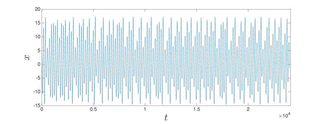
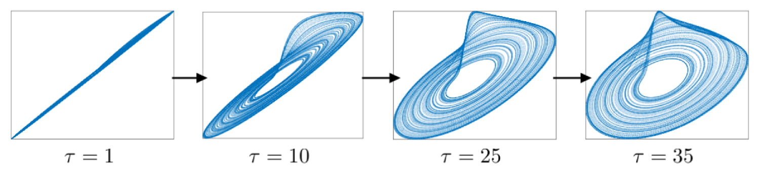
Figure 1: A time series from the Rossler system (top) and a number of delay-coordinate embeddings of that time series with different values of the delay parameter, $\tau$.

If $\tau$ is very small, the $m$ coordinates in each of these vectors are strongly correlated and so the embedded dynamics lie close to the main diagonal of the reconstruction space; as $\tau$ is increased, that reconstruction ‘unfolds’ off that subspace.

The original embedding theorems only require that $\tau$ be nonzero and not a multiple of any any orbit’s period. This is only valid, however, when one is using real-valued arithmetic on an infinite amount of noise-free data from perfect sensors. In practice—when noisy, finite-length time-series data and floating-point arithmetic are involved—one needs a higher $\tau$ to properly unfold the dynamics off the main diagonal. The $\tau=1$ embedding in Figure 1, for instance, will be indistinguishable from a diagonal line if its thickness is smaller than the measurement noise level. Since improperly unfolded reconstructions are not topologically conjugate to the true dynamics, this is a real problem. For this and other reasons, it can be a challenge to estimate good values for the $\tau$ parameter, as described in more depth in Section II.2.

The original embedding theorems also require $m>2d$ to assure topological conjugacy, where $d$ is the true dimension of the underlying dynamics. The trajectory crossings in the two-dimensional projection of the embedded Rossler data in Figure 1, for instance, do not exist in the real attractor, and so the two structures do not have the same topology. Sauer et al. Sauer, Yorke, and Casdagli (1991) loosened this requirement to $m>2d_{A}$, where $d_{A}$ is the capacity dimension of the attractor. In practice, however, $d$ is rarely known and $d_{A}$ cannot be calculated without first embedding the data. A large number of heuristic methods have been proposed to work around this quandary. Many of these methods are computationally expensive, most of them require significant interpretation by—and input from—a human expert, and all of them break down if one has a short or noisy time series. These methods, and their limitations, are also discussed in Section II.2.

There are two other requirements in the delay-coordinate embedding theorems, one of which is implicit in the formula above: that one has evenly spaced values of $y$. Data-acquisition systems do not have perfect time bases, so this can be a problem in practice. An obvious workaround here is interpolation, but then one is really studying a mix of real and interpolated dynamics. The final requirement is that the measurement process that produces $y$ is a smooth, generic function on the state space of the system. This will not be the case, for instance, if some event counter in the data-acquisition system overflows. It can be hard to know whether the measurement function satisfies the theoretical requirement; strategies for doing so include changing the sampling frequency or measuring a different quantity and then repeating the analysis. If the results do not change, one can be more confident that they are correct. Formal proofs of that correctness, of course, are not possible because of the nature of real-world data and digital computers.

Multivariate time-series data are useful for other reasons besides the corroboration that is afforded via individual analyses of different components. It is also possible to perform multi-element reconstructions that combine the information in those components. In their 1980 paperPackard et al. (1980), Packard et al. conjectured that any $m$ quantities that “…uniquely and smoothly label the states of the attractor” could serve as effective elements of a reconstruction-space vector. This powerful idea is used surprisingly rarely, even though it is fully supported by all routines of the tisean software packageHegger, Kantz, and Schreiber (1999). With the improvement of sensor technology, the dynamical analysis of multivariate data will likely become more important in the coming years, as discussed in Section V.

The kind of ‘due diligence’ exercise mentioned above is critical to the success of any nonlinear time-series analysis task. Data length, noise, nonstationarity, algorithm parameters, and the like have strong effects on the results, and the only way to know whether those effects are at work in one’s results is to repeat the analysis while manipulating the data (downsampling, for instance, or analyzing the first and last half of the data set separately) and the analysis parameters—the $m$ and $\tau$ values, the algorithmic scale parameters, etc. If one can also manipulate the experimental parameters, repeated analyses can reveal whether the data are sampled too coarsely in time to capture the details of the dynamics, or for too short a period to sample its overall structure.

II.2 Estimation of embedding parameters

The theoretical requirements on the embedding parameters—the delay $\tau$ and the embedding dimension $m$—are, as mentioned in the previous section, quite straightforward. In practice, however, one does not know the dimension of the system under study, nor does one have perfect data or a computer that uses infinite-precision arithmetic. Estimating good value for $m$ and $\tau$ in the face of these difficulties is one of the main challenges of delay-coordinate embedding. Dozens of methods for doing so have been developed in the past few decades; we will only cover a few representative members of this set.

In traditional practice, one chooses $\tau$ first, most often by computing a statistic that measures the independence of $\tau$-separated points in the time series. The first zero of the autocorrelation function of the time series, for instance, yields the smallest $\tau$ that maximizes the linear independence of the coordinates of the embedding vector; the first minima of the average mutual information Fraser and Swinney (1986) or the correlation sum Liebert and Schuster (1989); Grassberger and Procaccia (1983a) occur at $\tau$ values that maximize more-general forms of independence. (One wants the smallest $\tau$ that is reasonable because the reconstructed attractor can fold over on itself as $\tau$ grows, causing other problems.) There are also geometry-based strategies for estimating $\tau$ by, for example, examining the continuity on the reconstructed attractor or the amount of space that it fills. While there has been some theoretical discussionCasdagli et al. (1991) of what constitutes an optimal $\tau$, there are no universal strategies for putting those ideas into practice—especially since the process is system-dependent, and since a $\tau$ that works well for one purpose (e.g., prediction) may not work well for another (e.g., computing dynamical invariants).

After choosing a value for $\tau$, the next step is to estimate the embedding dimension $m$. As in the case of $\tau$, bigger is not necessarily better—since a single noisy point in the time series will affect $m$ of the points in an $m$-embedding—so one wants the smallest $m$ that affords a topologically correct result. There are two broad families of approaches to this, one based on the false near neighbor (FNN) algorithm of Kennel et al. Kennel, Brown, and Abarbanel (1992) and another that might be termed the “asymptotic invariant” approach. In the latter, one embeds the data for a range of dimensions, computes some dynamical invariant (e.g., those discussed in Section III), and selects the $m$ where the value of that invariant settles down. In an FNN-based method, one embeds the data, computes each point’s near neighbors, increases the embedding dimension, and repeats the near-neighbor calculation. If any of the relationships change—i.e., some neighbor in $k$ dimensions is no longer a neighbor in $k+1$ dimensions—that is taken as an indication that the dynamics were not properly unfolded with $m=k$. Noise also disturbs neighbor relationships, though, and thus can affect the operation of FNN-based algorithms. No member of either family of methods provides a guarantee, but both offer effective strategies for estimating $m$. Again, it can be very useful to employ several different methods to corroborate one’s results.

This two-step process is not the only approach. It has been noted that what really matters is the $m*\tau$ product—i.e., how much of the data are spanned by the embedding vector—and thus that estimating the two parameters at the same time, in combination, may be more effective Liebert, Pawelzik, and Schuster (1991); Pecora et al. (2007). It has also been suggested that one need not use the same $\tau$ across all $m$ coordinates of the embedding vector—i.e., that a systematically skewed embedding space may correspond better to the true dynamicsGrassberger, Schreiber, and Schaffrath (1991).

III Mathematical beauty: Characterization of the invariant measure

The invariant measure of a dynamical system can be characterized in a number of different ways: the fractal dimension of the invariant set, for instance, from the point of view of state-space geometry, or the Kolmogorov-Sinai (K-S) entropy if one is interested in uncertainty about the future of a chaotic trajectory. The stability with respect to infinitesimal perturbations can be quantified by the Lyapunov exponents. The topological equivalence guaranteed by the embedding theorems allows all of these quantities—and many others not mentioned here—to be determined from the time-series data.

III.0.1 Dimension estimates

There is a whole family of fractal dimensions $D_{q}$, usually called the Renyi dimensions. Their most intuitive definition is through a partitioning of the state space: the number of boxes $N_{\epsilon}$ of size $\epsilon$ needed to cover a fractal set with dimension $D_{0}$ scales with the box size $\epsilon$ as $\epsilon^{-D_{0}}$. This is an evident generalization of the integer dimensions, as one can easily verify: a line segment, for instance, will yield $D_{0}=1$ via this procedure, regardless of whether the surrounding space has two, three or more dimensions. $D_{0}$, often called the capacity dimension, is closely related to the Hausdorff dimension. For the generalized dimensions, one has to determine the measure on every box from the partition and raise that measure to the power $q$, with $\sum p_{i}^{q}\propto\epsilon^{(1-q)D_{q}}$ for $\epsilon\to 0$ and $p_{i}$ being the weight on the $i$th box.

Direct application of these box-counting methods to the points in the reconstructed state space is possible, but involves significant memory and processing demands and its results can be very sensitive to data length. A more-efficient, more-robust estimator of fractal dimensions is the Grassberger-Procaccia correlation sumGrassberger and Procaccia (1983b). We recall only the simplest version, which yields $D_{2}$. Rather than count boxes that are occupied by data points, one instead examines the scaling of the correlation sum as a function of $\epsilon$:

$$C_{2}(m,\epsilon):=\frac{1}{2N(N-T)}\sum_{i}\sum_{j<i-T}\Theta(\epsilon-||\vec{x}_{i}-\vec{x}_{j}||)\;,$$ (2)

where $\Theta$ is the Heaviside step function. $C_{2}(m,\epsilon)$ represents the fraction of pairs of data points in the $m$-dimensional embedding space whose spatial distance (measured by the Euclidean or maximum norm) is smaller than the scale $\epsilon$. This number scales as $\epsilon^{D_{2}}$ if $m>D_{2}$Sauer and Yorke (1993). The parameter $T$, going back to TheilerTheiler (1986), ensures that the temporal spacing between potential pairs of points is large enough to represent an independently identically distributed sample.

Formally, of course, the dimension of any finite point-set data should be zero. In the limit as $\epsilon\rightarrow 0$, methods that simply count occupied boxes correctly reflect this fact. In nonlinear time-series analysis, however, we are interested in the dimension of the set that is represented by the point-set data. The correlation sum provides an unbiased estimator for that quantity, and one that is accurate for small $\epsilon$—unlike the box method, which is strongly biased towards small $D$ values in this limitGrassberger (1988).

There is a conundrum involved in any estimation of the dimension of a delay-coordinate embedding, which is sometimes known as the conflict between redundancy and irrelevancyCasdagli et al. (1991). Specifically, in order to assure that successive elements of a delay vector are independent, the time lag $\tau$ should be sufficiently large. This can, however (as mentioned in the second paragraph of Section II.2) ‘overfold’ the reconstructed dynamics—especially if the embedding dimension is high. In these situations, it can require extremely well-sampled data in order to correctly resolve the folds and voids in complicated chaotic attractors. One can turn this reasoning around to estimate the number of data points $N$ needed to estimate the dimension of a data set; a pessimistic answer to this Olbrich and Kantz (1997) is $N\approx\sqrt{100^{D_{2}}e^{D_{2}h_{2}\tau}}$, where $h_{2}$ is the correlation entropy of the dynamics, $\tau$ the time delay of the reconstruction, and $e^{D_{2}h_{2}\tau}$ describes the effects of folding in the delay embedding space due to the minimal embedding dimension $m>D_{2}$. Among other things, this means that the number of points needed to estimate the dimension of chaotic dynamics reconstructed from a scalar time series is much larger than in the original state space, where the entropy factor can be ignored and $N>42^{D_{2}}$ has been suggestedSmith (1988).

III.0.2 Lyapunov exponents

Dimension estimate have pitfalls and caveats, but they are quite robust. Estimates of Lyapunov exponents are unstable. A number of creative strategies have been developed for estimating the full set of $m$ Lyapunov exponents $\lambda_{k}$ in the $m$-dimensional embedding space (e.g., Eckmann et al. (1986)); there are also many algorithms for estimating $\lambda_{1}$, the largest exponent, alone (e.g., Wolf et al. (1985); Sano and Sawada (1985)). Every one of these algorithms involves free parameters, however, and their results are often extremely sensitive to the values of those parameters—as well as to data length, noise, and the like. When working with reconstructed dynamics, one must also be aware of the issue of spurious exponents, since the number of Lyapunov exponents is equal to the number of dimensions in the ambient space. Scalar time-series data sampled from $D$-dimensional dynamical systems are typically embedded in $m$ dimensions with $m>D$, and those dynamics have $m$ Lyapunov exponents. Ideally, one would like to find $D$ exponents that correspond to those of the original dynamics—or at least to identify the $m-D$ extra ones that are spurious. There is a neat theory that predicts the numerical values of these spurious exponents in lowest-order approximationSauer, Tempkin, and Yorke (1998), but this cannot usually be reproduced in practice due to inaccessability of these scalesYang, Radons, and Kantz (2012).

III.0.3 The Kolmogorov-Sinai entropy

Theoretically, the K-S entropy (rate) $h_{KS}$ can be determined via Pesin’s identityPesin (1977), which states that it is the sum of the positive Lyapunov exponents. Since spurious exponents are hard to identify, though, and can even be positive, it is difficult to put this into practice in the context of embedded data (or to use the Kaplan-Yorke formula in order to determine the Lyapunov dimension). Rather, one typically estimates $h_{KS}$ through refined partitions, closely following its definition (e.g., Schuster and Just (2005)). The most straightforward implementation of this approach discretizes the space of joint probabilities and searches for sequences of successive delay vectors in specific sequences of boxes. As in the case of box-counting implementations of fractal dimension calculations, this can lead to underestimation: a sequence that exists in the underlying dynamics may not be ‘sampled’ by a given set of observations. In the box-counting implementation, every sequence with estimated probability 0 will systematically reduce the estimate of the K-S entropy. A way around this is to compute the correlation entropy (rate) $h_{2}$, which can be estimated by the correlation sum. To do this, one calculates Eq.(2) for a range of dimensions $m$ that are larger than the assumed minimum for an embedding, obtaining $h_{m}(\epsilon)=\ln C(m,\epsilon)-\ln C(m+1,\epsilon)$. Ideally, for some range of $\epsilon$, one should see a convergence of $h_{m}(\epsilon)\to h_{2}$ for large $m$. For a consistency check, one can then go back to Pesin’s identity and compare the estimate of $h_{2}$ to the sum of the positive Lyapunov exponents.

IV What practitioners need

A precise characterization of the invariant measure is not the goal of most time-series analyses; moreover, few real-world data sets are measured by perfect sensors operating on low-dimensional dynamics, which means that a proper determination of, e.g., Lyapunov exponents, is out of reach, anyway. In practice, one typically wants to describe a signal in some formalized manner, perhaps in order to discriminate between it and some other signal. Other important tasks include noise reduction, detection of changes in dynamical properties within a given signal, or prediction of its future values. In all of these situations, nonlinear time-series analysis has something to contribute.

IV.1 Signal and system characterization

A typical task is to characterize a single time series by a small set of numbers—for the purposes of classification, for instance, or comparison with other time series. Examples include medical diagnostics (is a patient healthy or sick?) or monitoring of machines (is a lathe bearing wearing out?). In these and many other important applications, nonlinear time-series analysis offers a large zoo of useful approaches, a few of which we describe below.

IV.1.1 Surrogate data

In cases where strong evidence for some property is missing, one must resort to statistical hypothesis testing. With a finite data set, one can never prove results about the underlying dynamics; one can only calculate probabilities that a particular finding is unprobable using a simple null hypothesis. This approach can provide some evidence that a more-complex (nonlinear, chaotic) dynamics is plausible, for instance.

In nonlinear time-series analysis, the test statistics—Lyapunov exponents, entropies, prediction errors, etc.—are complicated and their probability distributions under simple null hypotheses are typically unknown. Furthermore, the “simple” null hypotheses are typically not so simple. In the face of these challenges, one can proceed as follows. First, one chooses a particular statistical estimator (e.g., the violation of time inversion invarianceSchreiber and Schmitz (1997), which is a nonlinear property). Second, one determines its value $v_{d}$ on the target data set. Third, one interprets that value by comparing it to the distribution of values $v_{s}$ obtained from a large number of time series that fulfill a certain null hypothesis (e.g., of AR processes). Depending on where the computed value $v_{d}$ falls in this $v_{s}$ distribution, one can compute the probability of obtaining that value “by chance.” This provides a confidence level by which the null hypothesis can be rejected.

How does one obtain the distribution of the test statistics under the null hypothesis? This is where surrogate dataTheiler et al. (1991) enter the game. These are data that share certain properties of the time series under study and also fulfill a certain null hypothesis. The idea is that if one can produce a number of such surrogate time series, one can numerically compute the distribution of the test statistic on the null hypothesis. The critical questions here are

• which properties of the original data should be shared by the surrogates?

• what should the null hypothesis be?

Some of the answers are easy: since insufficient time-series length poses severe problems, the individual surrogate data sets should have the same length as the series under study. Others are not: ideally, for instance, each of these sequences should represent the same marginal probability distribution as the original data. Since a rather powerful null model is the class of ARMA models, it is reasonable to require the surrogate data to have the same power spectrum (more precisely, the same periodogram) as the original data—i.e., that temporal two-point correlations are identical. This is very useful when one wants to test for nonlinearities, which express themselves in nontrivial temporal $n$-point-correlations.

The technical way to create surrogate data with identical two-point correlations and identical marginal distributionSchreiber and Schmitz (1996) is to Fourier transform one’s original data, randomize the relative Fourier phases, back transform (this creates close-to-Gaussian random numbers with identical Fourier spectrum), and map the results onto the original time-series values by rank ordering. The third step restores the original marginal distribution but partly destroys the correlations, so the power spectrum has to be re-adjusted by Wiener filtering. Some iteration of these steps is generally required until the features of the surrogate data converge. See Schreiber and Schmitz (2000) for a careful discussion of this family of methods.

While surrogate data tests are very useful—and very different than the bootstrapping techniques used in other data-analysis fields—there are a number of caveats of which one must be aware when using them. Prominent among these is the nonstationarity trap: surrogates, by construction, are stationary, whereas the original data may be nonstationary. A difference in test statistics between surrogates and original data, then, might have its origin in nonstationarities rather than in nonlinearities.

IV.1.2 Permutation Entropy

Since the 1950s, entropy has been a well-established measure of the complexity and predictability of a time seriesShannon (1951). This is all very well in theory; in practice, however, estimating the entropy of an arbitrary, real-valued time series is a significant challenge. The K-S entropy, for instance, is defined as the supremum of the Shannon entropy rates of all partitions Petersen (1989), but not any partition will do for this computation. There are creative ways to work around this, as described in Section III.0.3. The main issue is discretization: these entropy calculations require categorical data—symbols drawn from a finite alphabet—but time-series data are usually real-valued and binning real-valued data from a dynamical system with anything other than a generating partition can destroy the correspondence between the true and symbolized dynamicsLind and Marcus (1995).

Permutation entropyBandt and Pompe (2002) is an elegant way to work around this problem. Rather than computing the statistics of sequences of categorical values, as in the calculation of K-S and Shannon entropy, permutation entropy considers the statistics of ordinal permutations of short subsequences of the time series. If $(x_{1},x_{2},x_{3})=(9,1,7)$, for example, then its ordinal pattern, $\phi(x_{1},x_{2},x_{3})$, is $231$ since $x_{2}\leq x_{3}\leq x_{1}$. The ordinal pattern of the permutation $(x_{1},x_{2},x_{3})=(9,7,1)$ is $321$. To compute the permutation entropy, one considers all the permutations $\pi$ in the set $\mathcal{S}_{n}$ of all $n!$ permutations of order $n$, determines the relative frequency with which they occur in the time series, $\{x_{t}\}_{t=1,\dots,T}$:

$$p(\pi)=\frac{\left|\{t|t\leq T-n,\phi(x_{t+1},\dots,x_{t+n})=\pi\}\right|}{T-n+1}$$

where $|\cdot|$ is set cardinality, and computes

$$H_{PE}(n)=-\sum_{\pi\in\mathcal{S}_{n}}p(\pi)\log_{2}p(\pi)$$

Like many algorithms in nonlinear time-series analysis, this calculation has a free parameter: the length $n$ of the subsequences used in the calculation. The key consideration in choosing it is that the value be large enough to expose forbidden ordinal patterns but small enough that reasonable statistics over the ordinals can be gathered from the given time series. When this value is chosen properly, permutation entropy can be a powerful tool; among other things, it is robust to noise, requires no knowledge of the underlying mechanisms, and is identical to the Shannon entropy for many large classes of systems Amigó (2012).

IV.1.3 Recurrence plots

A recurrence plotEckmann, Kamphorst, and Ruelle (1987) is a two-dimensional visualization of a sequential data set—essentially, a graphical representation of the recurrence matrix of that sequence. The pixels located at $(i,j)$ and $(j,i)$ on a recurrence plot (RP) are black if the distance between the $i^{th}$ and $j^{th}$ points in the time series falls within some threshold corridor

$$\delta_{l}<||\vec{x}_{i}-\vec{x}_{j}||<\delta_{h}$$

for some appropriate choice of norm, and white otherwise. These plots can be very beautiful, particularly in the case of chaotic signals; see Figure 2 for an example.

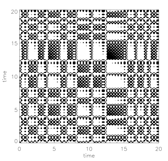
Figure 2: A signal and its recurrence plot. Reproduced with permission from Chaos. 2:596 (2002). Copyright 2002 AIP Publishing.

(There are also “unthresholded” RPs, which use color-coding schemes to represent a range of distances according to hue; these are even more striking.)

RPs are useful in that they bring out correlations at all scales in a manner that is obvious to the human eye, and they are one of the few analysis techniques that work with nonstationary time-series data, but their rich geometric structure—which, in the case of chaotic signals, is related to the unstable periodic orbits in the dynamicsBradley and Mantilla (2002)—can make them hard to interpret. Recurrence quantification analysis (RQA)Zbilut and Webber (1992) defines a number of quantitative metrics to describe this structure: the percentage of black points on the plot, for example, or the percentage of those black points that are contained in lines parallel to (but excluding) the main diagonal. RQA has been applied very successfully to many different kinds of time-series data, notably from physiological experiments (e.g., Webber and Zbilut (1994)). An extremely useful review article is Marwan et al. (2007).

IV.1.4 Network characteristics for time series

Recently, recurrence plots have been interpreted in a very different way, namely as the adjacency matrix of an undirected networkDonner et al. (2011). In this approach, an RP of an $N$-point time series is converted into a network of $N$ nodes, pairs of which are connected where the corresponding entries of the adjacency matrix are non-zero. One can then determine numerical values for different network characteristics, such as centrality, shortest path length, clustering coefficients, and many more. There are some evident questions, the most relevant being about the invariance of findings under variation of the threshold value $\delta_{l}$, since this value determines the link density of the network and all network characteristics become trivial in the limit of full connectivity.

IV.2 Prediction

Prediction strategies that work with state-space models have a long history—and a rich tradition—in nonlinear dynamics. The reconstruction machinery of Section II plays a critical role in these strategies, as it allows them to be brought to bear on the problem of predicting a scalar time seriesEckmann and Ruelle (1985). In 1969, for instance, Lorenz proposed his “Method of Analogues,” which searches the known state-space trajectory for the nearest neighbor of a given point and takes that neighbor’s forward path as the forecastLorenz (1969); not long after the original embedding papers, Pikovsky showed that the Method of Analogues also works in reconstructed state spacesPikovsky (1986).

Of course the canonical prediction example in deterministic nonlinear dynamics is the roulette work of the Chaos Cabal at the University of California at Santa Cruz, a project that not only catalyzed a lot of nonlinear science—including the original embedding paperPackard et al. (1980)—but also a lot of interest in the field from both scientific and lay communitiesBass (1992) that continues to this daySmall and Tse (2012).

In the decades since Lorenz’s Method of Analogues and the roulette project, a large number of creative strategies have been developed to predict the future course of a nonlinear dynamical systemCasdagli and Eubank (1992). Most of these methods build some flavor of local model in ‘patches’ of a reconstructed state space and then use that model to make the prediction of the next point. Early examples include Farmer and Sidorowich (1987); Smith (1988); Casdagli (1989); Sugihara and May (1990). This remains an active area of research and has even spawned a time-series prediction competitionWeigend and Gershenfeld (1993).

The Method of Analogues is not only applicable to deterministic dynamics. The short-term transition probability density of a Markov process depends only on the current state, which can be approximated by a delay vector. The “futures” of delay vectors from a small neighborhood can be viewed as a sample of the distribution, one time step ahead. This approach has been used for modelingPaparella et al. (1997) and predictingRagwitz and Kantz (2002) nonlinear stochastic processes.

Surprisingly, perfect embeddings are not required for successful predictions. In particular, reconstructions that do not satisfy the theoretical requirements on the embedding dimension $m$ can give prediction methods enough traction to match or even exceed the accuracy of the same methods working in a full embedding—particularly when the data are noisy Garland and Bradley (2015). One can then try to optimize, e.g., the embedding parameters. Of course, overfitting can be an issue in any prediction strategy; one must be careful not to fool oneself by over-optimizing a predictor to the given data.

IV.3 Noise and filtering

All real-world signals are contaminated by measurement noise. Most commonly, noise is treated as an additive random process on top of the true signal. Some forms of experimental apparatus contaminate the signal in different ways, however: “shot” noise, for instance, which appears only intermittently, or systematic bias in some measurement device. Regardless of its form, noise can interfere with nonlinear time-series analysis if it is too large—where “too large” depends greatly on the method that one wants to use.

Many studies in the literature are concerned with the fundamental issue of distinguishing chaos and noise (see Cencini et al. (2002) and references therein). This can be a real challenge. Both types of signals exhibit irregular temporal fluctuations, with a fast decay of the auto-correlation function, and both are hard to forecast. They differ in the dynamical origin of these features: chaos is a deterministic process, noise not. In a deterministic system, the short-term futures of two almost-identical states should be similar; in a pure noise process that is improbable. But, as mentioned above, noise takes on many forms. The simplest and most tractable is white noise: sequences of independently identically distributed (iid) random numbers. Their statistical independence, as expressed by the factorization of their joint probability distributions, can be easily identified by statistical tests.

If the noise is not additive, the challenge mounts. A noise-driven chaotic system—e.g., a nonlinear stochastic differential equation—produces something we might call noise. Mathematically speaking, such a system will, in any delay-coordinate embedding space, generate an invariant measure whose support has the full state-space dimension without fractal structure. In such a system, infinitesimally close trajectories will not diverge exponentially fast, but rather separate diffusively, at least on short time scales. Nonetheless, if such dynamical noise or interactive noise is sufficiently weak, one can still identify and characterize the deterministic properties of the system. However, there is often a smooth transition between chaos and noise, leaving the whole issue without a clear resolution.

It is, however, our impression that this issue is over-emphasized. In most time-series applications, it is not most critical to “distinguish between chaos and noise,” but rather to decide on the complexity of the process: whether is it linear or nonlinear, where it falls on the spectrum between redundancy and irrelevancy, etc. And then we are much better off, as there exist quite powerful tools for answering these questions (see, e.g., Sections IV.1.1 and IV.1.2).

Removing noise from a signal can also be a real challenge. Traditional filtering strategies discriminate between signal and noise using some sort of frequency threshold: e.g., removing all of the high-frequency components of the signal. In a chaotic signal, where the frequency spectrum is broad band, such a scheme will filter signal out along with the noiseTheiler and Eubank (1993). To be effective, filtering strategies for nonlinear time-series data must be tailored to and informed by the unique properties of nonlinear dynamics. One can, for instance, use the native geometry of the stable and unstable manifolds in a chaotic attractorFarmer and Sidorowich (1988) or local models of the dynamics on the attractorKostelich and Yorke (1988); Grassberger et al. (1993), to reduce noise. One can also exploit the topology of such attractors in nonlinear filtering schemesRobins, Rooney, and Bradley (2004).

IV.4 Issues and limitations

Nonlinear time-series analysis in the reconstructed state space is a powerful and useful idea, but it does has some practical limitations. These limitations are by no means fatal, but one has to be aware of them in order to report correct results.

In theory, delay-coordinate embedding is only guaranteed to work for an infinitely long noise-free observation of a single dynamical system. This poses a number of problems in practice, beginning with nonstationarity: embedding a time series gathered from a system that is undergoing bifurcations, for instance, will produce a topological stew of those different attractors. “Invariants” computed from such a structure, needless to say, will not accurately describe any of the associated dynamical regimes. One can use the tests described at the end of Section II.1 to determine whether these effects are at work in one’s results: e.g., repeating the analysis on different subsequences of the data and seeing if the results change. The recurrence plots described in Section IV.1.3 can also be helpful in these situations, allowing one to quickly see if different parts of the signal have different dynamical signatures.

The analysis of different subsequences of a time series has many other uses besides detecting nonstationarity, including determining whether or not one has enough data to support one’s analysis. The original embedding theorems require an infinite amount of data, but looser bounds have since been established for different problemsTsonis, Elsner, and Georgakakos (1993); Smith (1988); Eckmann and Ruelle (1992). It is important to know and attend to these limits; a computation of a Lyapunov exponent of a five-dimensional system from a data set that contains 100 points, for instance, should probably not be trusted. It is also important to keep these effects in mind when repeating analyses on subsets of one’s data, since the changes in the results that one wants to use as a diagnostic tool can simply be the result of short data lengths.

Dimension is a major practical issue for many reasons, not just because it is not known a priori and can be a challenge to estimate. Most of the results cited above regarding the data length that is necessary for success in nonlinear time-series analysis scale with the dimension of the dynamical system—often quite badly. This becomes even more of a challenge in spatially extended systems, where the state space is high (or even infinite) dimensional and the dynamics is spatio-temporal. In cases like this, the full attractor cannot be reconstructed by delay-coordinate embedding. This can in some cases be circumvented by exploiting homogeneity of the system, however: if the dynamics is translationally invariant, local dynamics can be reconstructed and used for predictionsM.Bär, Hegger, and Kantz (1999); Parlitz and Merkwirth (2000).

Noise effects also scale with dimension, since any noisy time-series point will affect $m$ of the points in an $m$-dimensional embedding of those data. The detection and filtering strategies mentioned in Section IV.3 can help with noise problems, and subsequence analysis can be used to explore whether the data are adequate to support the analysis, but in the end there is simply no way around not having enough data.

Delay-coordinate embedding, as formulated at the beginning of Section II, requires data that are evenly sampled in time. If this is not true, constructing the delay vector $\vec{R}$ is impossible without interpolation, which introduces spurious dynamics into the results. There is, however, an elegant way around this issue if the data consist of discrete events, like the spikes generated by a neuron: one simply embeds the inter-spike intervalsSauer (1995). The idea here is that if the spikes can be considered to be the result of an integrate-and-fire process, then their spacing is an effective proxy for the integral of the corresponding internal variable, and that is a wholly justifiable quantity to embed. Even without integrate-and-fire dynamics, one can interpret interspike intervals as a specific Poinaré map, which justifies their embeddingHegger and Kantz (1997). This also applies to the time series formed by all maxima (all minima) of the signal.

Even though for practical purposes it is quite handy, using the same value of $\tau$ in between successive elements of a delay vector may not be optimal. Indeed, using delay vectors of the form $y(t),y(t-\tau_{1}),y(t-\tau_{1}-\tau_{2}),....,y(t-\tau_{1}-\tau_{2}-\ldots-\tau_{m-1})$, with non-negative $\tau_{i}$, can introduce more time scales into the reconstruction, which has been shown to be useful in many situationsPecora et al. (2007); Holstein and Kantz (2009). Such strategies might be also a way to tackle signals from multi-scale dynamics: if there are different time and length scales involved, a fixed $\tau$ may be too large to resolve the short ones and/or too small to resolve the long ones. This is particularly evident when embedding a human ECG signal: using standard delay vectors, one can either unfold the QRS complex or represent the t-wave as a loop, but not both.

V Perspectives

When getting involved in time-series analysis some 25 years ago, we could not have anticipated the wealth of data that would be available in 2015, facilitated by cheap and powerful sensors for all sorts of quantities, data-acquisition systems with sub-microsecond sampling rates and terabytes of memory, widespread remote-sensing technology, and incredible sense/compute power in small devices carried by the majority of the population of Earth. Commercial hardware and software are available to monitor all kinds of things, from physiological parameters obtained during daily activity by watch-sized objects to real-time traffic flows gathered by cameras on highways. These data can be used to suggest life-changing health interventions, produce routing suggestions to avoid traffic jams that have not yet formed, and the like.

All this involves data analysis: often, time-series analysis. The bulk of the techniques used in the various academic and commercial communities that are concerned with this problem—data mining, machine learning, and the like—are linear and statistical. Analysis techniques that accommodate nonlinearity and determinism could be an extremely important weapon in this arsenal, but nonlinear time-series analysis is currently underused outside the field of nonlinear science. (Of course, much of this software is proprietary, so one must be careful about such generalizations; nonlinear time-series analysis may already be running on Google’s computers and it would be hard for those outside the company to know.)

There are some serious barriers for the movement of nonlinear time-series analysis beyond the university desks of physicists and into widespread professional practice, however. Linear techniques have a long history and are taught in most academic programs. They are comparatively easy to use and they almost always produce answers. Whether or not those answers are correct, or meaningful, is a serious issue: cf., the discussion in Section I of the mean of a bimodal distribution. But to a community that is familiar with these linear techniques, the notion of learning a whole new methodology—one that relies on more-complex mathematics and only works if the data are good and the algorithm parameters are set right—can be daunting. One of us (EB) encountered significant resistance when attempting to convince the computer systems community to attend to nonlinearity and chaos in computer dynamics—an effect that could significantly impact the designs of those systems. Only when those effects become apparent and meaningful to those communities will nonlinear time-series analysis become more widespread. Another relevant issue here is whether low-dimensional deterministic dynamics is a good data model for broader use. So the only prediction that we make here is that nonlinear time-series analysis is still far from its culmination point, in terms of application.

What will be the relevant issues concerning the methodology itself? Here we can only speculate. It is evident that nonstationarity is still a major problem and many of its facets are not fully explored. Change-point detection is one of these. Distilling causality relationships from data is another critical open problem in nonlinear time-series analysis (e.g., couplings in climate science). Will this ever be possible? It is hard to say. On the algorithmic end of things, the various free parameters—and the sensitivity of the results to their values—are important issues. Will it be possible to design algorithms whose free parameters can be chosen systematically, via intuition, or perhaps even automatically? Such developments would streamline nonlinear time-series analysis, making it an indispensible tool to make sense out of the real world.

References

- Box and Jenkins (1976) G. E. P. Box and F. M. Jenkins, Time Series Analysis: Forecasting and Control (Holden Day, 1976) second edition.
- Hurst (1951) H. Hurst, “Long-term storage of water reserviors,” Transactions of the American Society of Civil Engineers 116 (1951).
- Peng et al. (1994) C. Peng, S. Buldyrev, S. Havlin, M. Simons, H. Stanley, and A. Goldberger, “Mosaic organization of DNA nucleotides,” Physical Review E 49, 1685 (1994).
- Abarbanel (1996) H. Abarbanel, Analysis of Observed Chaotic Data (Springer, 1996).
- Kantz and Schreiber (2004) H. Kantz and T. Schreiber, Nonlinear Time Series Analysis (Cambridge University Press, 2004).
- Crutchfield (1979) J. Crutchfield, “Prediction and stability in classical mechanics,” (1979), senior thesis in physics and mathematics, University of California, Santa Cruz.
- Packard et al. (1980) N. Packard, J. Crutchfield, J. Farmer, and R. Shaw, “Geometry from a time series,” Physical Review Letters 45, 712 (1980).
- Takens (1981) F. Takens, “Detecting strange attractors in fluid turbulence,” in Dynamical Systems and Turbulence, edited by D. Rand and L.-S. Young (Springer, Berlin, 1981) pp. 366–381.
- Sauer, Yorke, and Casdagli (1991) T. Sauer, J. Yorke, and M. Casdagli, “Embedology,” Journal of Statistical Physics 65, 579–616 (1991).
- Hegger, Kantz, and Schreiber (1999) R. Hegger, H. Kantz, and T. Schreiber, “Practical implementation of nonlinear time series methods: The TISEAN package,” Chaos: An Interdisciplinary Journal of Nonlinear Science 9, 413–435 (1999).
- Fraser and Swinney (1986) A. Fraser and H. Swinney, “Independent coordinates for strange attractors from mutual information,” Physical Review A 33, 1134–1140 (1986).
- Liebert and Schuster (1989) W. Liebert and H. Schuster, “Proper choice of the time delay for the analysis of chaotic time series,” Physics Letters A 142, 107–111 (1989).
- Grassberger and Procaccia (1983a) P. Grassberger and I. Procaccia, “Measuring the strangeness of strange attractors,” Physica D 9, 189–208 (1983a).
- Casdagli et al. (1991) M. Casdagli, S. Eubank, J. Farmer, and J. Gibson, “State space reconstruction in the presence of noise,” Physica D 51, 52–98 (1991).
- Kennel, Brown, and Abarbanel (1992) M. B. Kennel, R. Brown, and H. D. I. Abarbanel, “Determining minimum embedding dimension using a geometrical construction,” Physical Review A 45, 3403–3411 (1992).
- Liebert, Pawelzik, and Schuster (1991) W. Liebert, K. Pawelzik, and H. Schuster, “Optimal embeddings of chaotic attractors from topological considerations,” Europhysics Letters 14, 521 (1991).
- Pecora et al. (2007) L. Pecora, L. Moniz, J. Nichols, and T. Carroll, “A unified approach to attractor reconstruction,” Chaos: An Interdisciplinary Journal of Nonlinear Science 17, 013110 (2007).
- Grassberger, Schreiber, and Schaffrath (1991) P. Grassberger, T. Schreiber, and C. Schaffrath, “Nonlinear time sequence analysis,” International Journal of Bifurcation and Chaos 1, 521 (1991).
- Grassberger and Procaccia (1983b) P. Grassberger and I. Procaccia, “Measuring the strangeness of strange attractors,” Physica D 9, 189 (1983b).
- Sauer and Yorke (1993) T. Sauer and J. Yorke, “How many delay coordinates do you need?” International Journal of Bifurcation and Chaos 3, 737 (1993).
- Theiler (1986) J. Theiler, “Spurious dimension from correlation algorithms applied to limited time series data,” Physical Review E 34, 2427 (1986).
- Grassberger (1988) P. Grassberger, “Finite sample corrections to entropy and dimension estimates,” Physics Letters A 128, 369 (1988).
- Olbrich and Kantz (1997) E. Olbrich and H. Kantz, “Inferring chaotic dynamics from time series: On which length scale determinism becomes visible,” Physics Letters A 232, 63–69 (1997).
- Smith (1988) L. Smith, “Intrinsic limits on dimension calculations,” Physics Letters A 133, 283–288 (1988).
- Eckmann et al. (1986) J. Eckmann, S. Oliffson-Kamphorst, D. Ruelle, and S. Ciliberto, “Lyapunov exponents from time series,” Physical Review A 34, 4971 (1986).
- Wolf et al. (1985) A. Wolf, J. Swift, H. Swinney, and J. Vastano, “Determining Lyapunov exponents from time series,” Physica D 16, 285 (1985).
- Sano and Sawada (1985) M. Sano and Y. Sawada, “Measurement of the Lyapunov spectrum from a chaotic time series,” Physical Review Letters 55, 1091 (1985).
- Sauer, Tempkin, and Yorke (1998) T. Sauer, J. Tempkin, and J. Yorke, “Spurious Lyapunov exponents in attractor reconstruction,” Physical Review Letters 81, 4341 (1998).
- Yang, Radons, and Kantz (2012) H.-L. Yang, G. Radons, and H. Kantz, “Covariant Lyapunov vectors from reconstructed dynamics: The geometry behind true and spurious Lyapunov exponents,” Physical Review Letters 109, 244101 (2012).
- Pesin (1977) Y. Pesin, “Characteristic Lyapunov exponents and smooth ergodic theory,” Russian Mathematical Surveys. 32, 55 (1977).
- Schuster and Just (2005) H. Schuster and W. Just, Deterministic chaos (Wiley, 2005).
- Schreiber and Schmitz (1997) T. Schreiber and A. Schmitz, “Discriminating power of measures for nonlinearity in a time series,” Physical Review E 55, 5443 (1997).
- Theiler et al. (1991) J. Theiler, S. Eubank, A. Longtin, B. Galdrikian, and J. Farmer, “Testing for nonlinearity in time series: The method of surrogate data,” Physica D 58, 72–94 (1991).
- Schreiber and Schmitz (1996) T. Schreiber and A. Schmitz, “Improved surrogate data for nonlinearity tests,” Physical Review Letters 77, 635 (1996).
- Schreiber and Schmitz (2000) T. Schreiber and A. Schmitz, “Surrogate time series,” Physica D 142, 346–382 (2000).
- Shannon (1951) C. E. Shannon, “Prediction and entropy of printed English,” Bell System Techical Journal 30, 50–64 (1951).
- Petersen (1989) H. Petersen, Ergodic Theory (Cambridge University Press, 1989).
- Lind and Marcus (1995) D. Lind and B. Marcus, An Introduction to Symbolic Dynamics and Coding (Cambridge University Press, 1995).
- Bandt and Pompe (2002) C. Bandt and B. Pompe, “Permutation entropy: A natural complexity measure for time series,” Physical Review Letters 88, 174102 (2002).
- Amigó (2012) J. Amigó, Permutation Complexity in Dynamical Systems: Ordinal Patterns, Permutation Entropy and All That (Springer, 2012).
- Eckmann, Kamphorst, and Ruelle (1987) J.-P. Eckmann, S. Kamphorst, and D. Ruelle, “Recurrence plots of dynamical systems,” Europhysics Letters 4, 973–977 (1987).
- Bradley and Mantilla (2002) E. Bradley and R. Mantilla, “Recurrence plots and unstable periodic orbits,” Chaos: An Interdisciplinary Journal of Nonlinear Science 12, 596–600 (2002).
- Zbilut and Webber (1992) J. Zbilut and C. Webber, “Embeddings and delays as derived from recurrence quantification analysis,” Physics Letters A 171, 199–203 (1992).
- Webber and Zbilut (1994) C. Webber and J. Zbilut, “Dynamical assessment of physiological systems and states using recurrence plot strategies,” Journal of Applied Physiology 76, 965–973 (1994).
- Marwan et al. (2007) N. Marwan, M. Romano, M. Thiel, and J. Kurths, “Recurrence plots for the analysis of complex systems,” Physics Reports 438, 237 (2007).
- Donner et al. (2011) R. Donner, M. Small, J. Donges, N. Marwan, Y. Zou, R. Xiang, and J. Kurths, “Recurrence-based time series analysis by means of complex network methods,” International Journal of Bifurcation and Chaos 21, 1019–1046 (2011).
- Eckmann and Ruelle (1985) J.-P. Eckmann and D. Ruelle, “Ergodic theory of chaos and strange attractors,” Reviews of Modern Physics 57, 617 (1985).
- Lorenz (1969) E. Lorenz, “Atmospheric predictability as revealed by naturally occurring analogues,” Journal of the Atmospheric Sciences 26, 636–646 (1969).
- Pikovsky (1986) A. Pikovsky, “Noise filtering in the discrete time dynamical systems,” Soviet Journal of Communications Technology and Electronics 31, 911–914 (1986).
- Bass (1992) T. Bass, The Eudaemonic Pie (Penguin, New York, 1992).
- Small and Tse (2012) M. Small and C. Tse, “Predicting the outcome of roulette,” Chaos: An Interdisciplinary Journal of Nonlinear Science 22, 033150 (2012).
- Casdagli and Eubank (1992) M. Casdagli and S. Eubank, eds., Nonlinear Modeling and Forecasting (Addison Wesley, 1992).
- Farmer and Sidorowich (1987) J. Farmer and J. Sidorowich, “Predicting chaotic time series,” Physical Review Letters 59, 845–848 (1987).
- Casdagli (1989) M. Casdagli, “Nonlinear prediction of chaotic time series,” Physica D 35, 335–356 (1989).
- Sugihara and May (1990) G. Sugihara and R. May, “Nonlinear forecasting as a way of distinguishing chaos from measurement error in time series,” Nature 344, 734–741 (1990).
- Weigend and Gershenfeld (1993) A. Weigend and N. Gershenfeld, eds., Time Series Prediction: Forecasting the Future and Understanding the Past (Santa Fe Institute Studies in the Sciences of Complexity, Santa Fe, NM, 1993).
- Paparella et al. (1997) F. Paparella, A. Provenzale, L. Smith, C. Taricco, and R. Vio, “Local random analogue prediction of nonlinear processes,” Physics Letters A 235, 233–240 (1997).
- Ragwitz and Kantz (2002) M. Ragwitz and H. Kantz, “Markov models from data by simple nonlinear time series predictors in delay embedding spaces,” Physical Review E 65, 056201 (2002).
- Garland and Bradley (2015) J. Garland and E. Bradley, “Prediction in projection,” (2015), arxiv.org/abs/1503.01678.
- Cencini et al. (2002) M. Cencini, M. Falcioni, E. Olbrich, H. Kantz, and A. Vulpiani, “Chaos or noise: Difficulties of a distinction,” Physical Review E 62, 427 (2002).
- Theiler and Eubank (1993) J. Theiler and S. Eubank, “Don’t bleach chaotic data,” Chaos: An Interdisciplinary Journal of Nonlinear Science 3, 771–782 (1993).
- Farmer and Sidorowich (1988) J. Farmer and J. Sidorowich, “Exploiting chaos to predict the future and reduce noise,” in Evolution, Learning and Cognition (World Scientific, 1988).
- Kostelich and Yorke (1988) E. Kostelich and J. Yorke, “Noise reduction in dynamical systems,” Physical Review A 38, 1649–1652 (1988).
- Grassberger et al. (1993) P. Grassberger, R. Hegger, H. Kantz, C. Schaffrath, and T. Schreiber, “On noise reduction methods for chaotic data,” Chaos: An Interdisciplinary Journal of Nonlinear Science 3, 127 (1993).
- Robins, Rooney, and Bradley (2004) V. Robins, N. Rooney, and E. Bradley, “Topology-based signal separation,” Chaos: An Interdisciplinary Journal of Nonlinear Science 14, 305–316 (2004).
- Tsonis, Elsner, and Georgakakos (1993) A. Tsonis, J. Elsner, and K. Georgakakos, “Estimating the dimension of weather and climate attractors: Important issues about the procedure and interpretation,” Journal of the Atmospheric Sciences 50, 2549–2555 (1993).
- Eckmann and Ruelle (1992) J.-P. Eckmann and D. Ruelle, “Fundamental limitations for estimating dimensions and Lyapunov exponents in dynamical systems,” Physica D 56, 185–187 (1992).
- M.Bär, Hegger, and Kantz (1999) M.Bär, R. Hegger, and H. Kantz, “Fitting partial differential equations to space-time dynamics,” Physical Review E 59, 337 (1999).
- Parlitz and Merkwirth (2000) U. Parlitz and C. Merkwirth, “Prediction of spatiotemporal time series based on reconstructed local states,” Physical Review Letters 84, 1890 (2000).
- Sauer (1995) T. Sauer, “Interspike interval embedding of chaotic signals,” Chaos: An Interdisciplinary Journal of Nonlinear Science 5, 127 (1995).
- Hegger and Kantz (1997) R. Hegger and H. Kantz, “Embedding of sequences of time intervals,” Europhysics Letters 38, 267–272 (1997).
- Holstein and Kantz (2009) D. Holstein and H. Kantz, “Optimal Markov approximations and generalized embeddings,” Physical Review E 79, 056202 (2009).
- Aurell et al. (1997) E. Aurell, G. Boffetta, A. Crisanti, G. Paladin, and A. Vulpiani, “Predictability in the large: An extension of the concept of Lyapunov exponent,” Journal of Physics A: Mathematics and General 30, 1 (1997).