Holographic operator mapping in dS/CFT and cluster decomposition

Abstract

The bulk to boundary mapping for massive scalar fields is constructed, providing a de Sitter analog of the LSZ reduction formula. The set of boundary correlators thus obtained defines a potentially new class of conformal field theories based on principal series representations of the global conformal group. Conversely, we show bulk field operators in de Sitter may be reconstructed from boundary operators. While consistent at the level of the free field theory, the boundary CFT does not satisfy cluster decomposition. The resulting conformal field theory does not satisfy the basic axioms of Euclidean quantum field theory due to Osterwalder and Schrader, so is likely not well-defined once interactions are included.

I Introduction

The Bekenstein-Hawking entropy (Bekenstein, 1973; Hawking, 1975)

$$S=\frac{A}{4G}\,,$$

states that the entropy of any black hole is proportional to its surface area. This is law widely applicable in various kinds of spacetime. This law suggests that any theory in the bulk can be described in terms of some boundary theory of spacetime in one lesser dimension.

There has been a lot of progress in understanding this correspondence between bulk quantum theory in anti-de Sitter spacetime and boundary conformal field theory (Aharony et al., 2000). One expects these ideas to carry over in some form to the cases of asymptotically flat spacetime and asymptotically de Sitter spacetime. In these cases the situation is much less clear, and our aim in the present work is to carefully set up the bulk/boundary correspondence in the de Sitter case. This will allow us to draw some interesting conclusions about the structure of the novel conformal field theories that must appear in this case, and their ultimate consistency.

Various different formulations of dS/CFT has been proposed, following Strominger’s initial work (Strominger, 2001). Some formulations simply extend the AdS/CFT correspondence to the dS space via analytic continuation, which has been successful for massless fields (and possibly sub-Hubble mass fields) and the massless higher spin gravity theories (Anninos et al., 2011). Our goal in the present work is to investigate the situation for generic fields with masses larger than the Hubble scale, which are related by analytic continuation to tachyonic fields in anti-de Sitter spacetime. New methods must be developed to treat this case. It is worth noting that in the CFT these fields will correspond to quasi-primary fields with complex conformal weights. Nevertheless, these form unitary representations of the global conformal group (Chernikov and Tagirov, 1968; Tagirov, 1973; Güijosa and Lowe, 2004; Güijosa et al., 2005), opening the door to possibility that an entirely new class of conformal field theories might be defined based on these representations.

One of the key mysteries in the dS/CFT correspondence is the origin of bulk time, since the dual CFT is a purely Euclidean theory. In the AdS/CFT correspondence this is not an issue because the bulk time is parallel to the boundary time and the CFT lives in a spacetime with Lorentzian signature. As a result, it becomes more interesting to see how unitarity and time ordering in the bulk theory emerges from the Euclidean CFT, and we will obtain partial results in this direction.

The paper is organized as follows. We begin by presenting an analog of the LSZ construction (Lehmann et al., 1955) for quantum fields in de Sitter spacetime, which provides a clear definition of correlators in the boundary CFT. This step is necessary because the representations of the conformal group in question, the principal series, are not commonly studied in the context of conformal field theory. The construction is inspired by the integral geometry approach of Gelfand (Gel’fand et al., 1966), and many of the results detailed there carry over to the present case. For the most part, our focus will be on three-dimensional de Sitter spacetime, though many of the ideas carry over to the higher dimensional case.

We then consider the inverse map, reconstructing bulk field operators in terms of the CFT data. At leading order (essentially the free level from the viewpoint of quantum field theory in the bulk) we construct bulk creation and annihilation field operators using operators in the CFT. Bulk operator ordering in correlators can be accomplished by adopting an $i\epsilon$-prescription, complexifying the radial direction in the CFT. This is sufficient to recover the bulk Wightman two-point correlation function, with the correct Hadamard singularity at light-like separations. This approach may also be used to build higher point correlators, for bulk theories with perturbative expansions, by using the creation and annihilation operators to reproduce the Wick expansion. However a completely general nonperturbative understanding of the bulk operator ordering, and hence the origin of bulk time, is elusive.

The construction we describe allows one to define a CFT from some set of bulk correlators in de Sitter spacetime. We may then proceed to analyze the basic consistency of the resulting CFT, to check whether it satisfies the basic axioms expected of a Euclidean quantum field theory. These are known as the Osterwalder-Schrader axioms (Osterwalder and Schrader, 1973, 1975). One of these axioms is the Euclidean version of cluster decomposition, which requires correlators to factorize in the limit of large separations. We find this fails in the case of the principal series, if, for example, operators of the form $L_{1}\bar{L}_{1}\mathcal{O}_{\Delta}$ are considered, where $L_{1}$ and $\bar{L}_{1}$ are conformal generators that raise the weight by $1$, and $\mathcal{O}_{\Delta}$ is a quasi-primary operator with weight $\Delta$. Note in ordinary CFTs with $\mathcal{O}_{\Delta}$ a primary field with positive conformal weight, the combination $L_{1}\mathcal{O}_{\Delta}$ would vanish. The operator $L_{1}\bar{L}_{1}\mathcal{O}_{\Delta}$ will be dual to a graviton plus a massive matter field insertion. The failure of cluster decomposition signals that the vacuum of the CFT is not unique, i.e. there can be many excitations in the bulk that give rise to nontrivial operators on the boundary satisfying $L_{0}=\bar{L}_{0}=0$. This follows from the lack of a positive energy theorem in the bulk theory (Abbott and Deser, 1982),. We note this does not immediately imply infrared divergences in the bulk theory. In fact, the classical stability of de Sitter spacetime for pure gravity or massless conformal matter coupled to gravity has been demonstrated (Friedrich, 1986a, b, 1991). Most likely, this result should be interpreted as an incompleteness in the CFT dual to an interacting theory in de Sitter spacetime, a point we hope to return to in future work.

A related construction of bulk operators from boundary operators in dS/CFT has been considered in (Xiao, 2014; Sarkar and Xiao, 2015). There are numerous differences in the details and conclusions with the present work.

II Basic setup

In this section we will introduce some notation, broadly following the integral geometry approach of (Gel’fand et al., 1966) in imaginary Lobachevskian space, also known as elliptic de Sitter spacetime (Folacci and Sanchez, 1987; Parikh et al., 2003). Elliptic de Sitter is simply global de Sitter modulo the antipodal map. Our main focus will be global de Sitter. In some ways elliptic de Sitter is simpler because there is a single connected boundary at infinity, while in global de Sitter there are two disconnected boundaries, one in the distant past, and one in the distant future. We will find in global de Sitter a CFT may be defined on either boundary, and for the sake of definiteness we choose the past boundary. Our formulas will be explicitly written for the case of three-dimensional de Sitter spacetime, but the results generalize immediately to higher dimensions.

The de-Sitter space can be realized on a hyperboloid embedded in four-dimensional Minkowski spacetime

$$x_{0}^{2}-x_{1}^{2}-x_{2}^{2}-x_{3}^{2}=-R^{2}\,,$$ (1)

where $R$ is some positive constant. The geodesic distance $r$ between any two points

$$\cosh^{2}kr=\frac{\left\langle x,y\right\rangle^{2}}{\left\langle x,x\right\rangle\left\langle y,y\right\rangle}\,,$$ (2)

where

$$\left\langle x,y\right\rangle=x_{0}y_{0}-x_{1}y_{1}-x_{2}y_{2}-x_{3}y_{3}\,,$$

is the inner product of two vectors and $k=\frac{1}{R}$ is another positive constant.

The family of points satisfying $\left\langle x,x\right\rangle=-R^{2}$ with antipodal points ($x\sim-x$) identified is called imaginary Lobachevskian space or elliptic de Sitter spacetime. Without the identification we have ordinary global de Sitter spacetime. The distance $r$ can be real and non-negative (if $1\leq\cosh kr\leq\infty$) or imaginary in the interval $[0,\frac{\pi i}{2k}]$ (if $0\leq\cosh kr\leq 1$). Any point on the light cone in the embedding space will be denoted by $\xi$, that is $[\xi,\xi]=0$.

Now let us consider some surfaces in de Sitter with particularly simple transformation properties under the isometry group. The equation describing a sphere of radius $r$ with center at $a$ is given by

$$\left\langle x,a\right\rangle{}^{2}=c\left\langle a,a\right\rangle\left\langle x,x\right\rangle\,.$$

Consider taking the center to the infinity while ensuring that the sphere passes through a fixed point $b$. The surface obtained in this way is called a horosphere. In this limit, the product $c\left\langle a,a\right\rangle$ is fixed to some constant $c_{1}$ to obtain the surface

$$\left\langle x,\xi\right\rangle{}^{2}=c_{1}\left\langle x,x\right\rangle\,.$$ (3)

When $c_{1}<0$ this is called a horosphere of the first kind. It is possible to normalize $c_{1}=-1$ by normalizing $\xi$. If we set $R=1$, so that $\left\langle x,x\right\rangle=-1$ then the horospheres of the first kind look like

$$|\left\langle x,\xi\right\rangle|=1\,.$$ (4)

Thus a horosphere of the first kind may be specified by choosing a point $\xi$ on the positive cone, $\left\langle\xi,\xi\right\rangle=0\,,\xi_{0}>0$.

When $c_{1}=0$ one gets a horosphere of the second kind

$$\left\langle x,\xi\right\rangle=0\,.$$ (5)

In this paper, our focus will be on the horospheres of the first kind, which will correspond to principal series representations of the de Sitter group (Gel’fand et al., 1966). We consider further the horospheres of the second kind, which correspond to the discrete series representations, in future work.

III Boundary CFT operators

It is useful to begin by reviewing the decomposition of some general bounded, normalizable function on de Sitter into components that transform as unitary irreducible representations of the conformal group (Gel’fand et al., 1966). For every $f(x)$ one constructs the integral transform

$$h(\omega)=\int_{\omega}f(x)d\sigma\,,$$ (6)

and $d\sigma$ is an invariant measure, and the integral is over a horosphere of first kind $\omega$. Let the equation of a horosphere be $|\left\langle x,\xi\right\rangle|=1$. Equation (6) can also be written as

$$h(\xi)=\int f(x)\delta\left(|\left\langle x,\xi\right\rangle|-1\right)dx\,,$$ (7)

where $dx$ is the invariant measure on the de Sitter spacetime. This above map is nothing but a generalization of the Fourier transform, which takes a function defined on the horosphere to a function defined on the lightcone labelled by $\xi$. As we will see, $\xi$ can be used to parametrize the boundary at past infinity in de Sitter.

Now consider functions $h(\xi)$ over the positive sheet of the light cone where $\xi^{0}>0$. These functions may be decomposed into components with well-defined conformal weights by Fourier transforming

$$F(\xi;\rho)=\int_{0}^{\infty}h(t\xi)t^{-i\rho}dt\,,$$ (8)

where the complex conformal weight $\Delta$ is related to the real parameter $\rho$ via $i\rho=1-\Delta$. Let us note that inserting (7) into (8) we have

$$F(\xi;\rho)=\int_{0}^{\infty}dt\int dxf(x)\delta\left(\left|\left\langle x,t\xi\right\rangle\right|-1\right)t^{-i\rho}\,.$$

Performing the integral over $t$ we arrive at

$$F(\xi;\rho)=\int dxf(x)\left|\left\langle x,\xi\right\rangle\right|^{-\Delta}\,.$$ (9)

Generalizing $f$ to some bulk correlator of some scalar field of mass $m$, our goal will then be to view the analog of $F$ as a boundary correlator. A key difference with the work of Gelfand is that we must give up the condition of normalizability (in the sense that $\int|f(x)|^{2}dx$ is finite). As we will see, this the de Sitter isometry covariant component of (7) will correspond to the residue of a pole in $\rho^{2}-m^{2}$ reminiscent of the LSZ reduction formula in flat spacetime (Lehmann et al., 1955).

III.1 Flat slicing

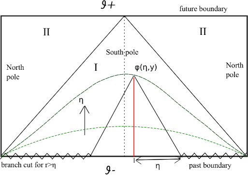
Figure 1: Penrose diagram for de-Sitter space. The vertical dashed line is the South pole. The left and right edges are North pole which are identified with each other. Horizontal dashed lines are constant $\eta$ slices. The figure shows the calculation of bulk field from boundary operator in the past boundary. The boundary operator is smeared over the whole boundary. There is branch cut in the smearing function for $r>\eta$. Continuing $r$ and $\eta$ to the complex plane via an $i\epsilon$ prescription selects the branch yielding a Bunch-Davies/Euclidean vacuum positive or negative frequency mode.

Horospheres of the first kind are diffeomorphic to flat spatial slices in de Sitter. It therefore will be convenient to express the general coordinate invariant expression (9) on flat slices. See (Drechsler and Sasaki, 1978) for some related work in the context of four-dimensional de Sitter. Setting $R=1$, the 3-dimensional de Sitter hyperboloid can be parameterized by the coordinates $(\eta,y_{1},y_{2})$ via

$$x^{0} = \frac{1}{2}(\eta-\frac{1}{\eta})-\frac{\sum y_{i}^{2}}{2\eta}$$

$$x^{1} = \frac{y_{1}}{\eta}$$

$$x^{2} = \frac{y_{2}}{\eta}$$

$$x^{3} = -\frac{1}{2}(\eta+\frac{1}{\eta})+\frac{\sum y_{i}^{2}}{2\eta}\,,$$

yielding the de Sitter metric with a flat spatial slicing and conformal time $\eta$

$$ds^{2}=\frac{d\eta^{2}}{\eta^{2}}-\frac{1}{\eta^{2}}\left(dy_{1}^{2}+dy_{2}^{2}\right)\,.$$

The volume measure is

$$dx=\frac{1}{\eta^{3}}d\eta dy_{1}dy_{2}\,.$$ (10)

A point on a light cone may be parameterized by

$$\xi=k\lambda(1+z^{2},2z_{1},2z_{2},1-z^{2})\,,$$ (11)

where $z^{2}=z_{1}^{2}+z_{2}^{2}$. The coordinates $z_{1},z_{2}$ label a point on the boundary at past infinity in de Sitter. In these coordinates we have

$$\left\langle x,\xi\right\rangle=\lambda\eta\left(1-\frac{(y_{1}+z_{1})^{2}}{\eta^{2}}-\frac{(y_{2}+z_{2})^{2}}{\eta^{2}}\right)\,.$$

We will also need the measure on the cone

$$d\xi=\frac{d\xi_{1}d\xi_{2}d\xi_{3}}{\xi_{0}}\,,$$

and the measure on the boundary at infinity

$$d\omega=d^{2}z\,.$$

III.2 Transform from bulk to boundary

Our aim is to use the transform of Gelfand (Gel’fand et al., 1966) as a guide to constructing the transform for the class of functions that appear in correlation functions of quantum fields in de Sitter. In particular, these functions do not satisfy the compact support condition used in Gelfand’s inversion theorem. This will lead us to build an analog of the flat-spacetime LSZ reduction formula for de Sitter spacetime, requiring some important differences with Gelfand’s construction.

We begin by noting the mode expansion for a bulk scalar field of mass $m$ (Birrell and Davies, 1982)

$$\phi(\eta,y)=c_{1}\int\frac{d^{2}k}{(2\pi)^{2}}\left(a_{k}\eta H_{i\mu}^{(2)}\left(|k|\eta\right)e^{ik.y}+a_{k}^{\dagger}\eta H_{i\mu}^{*(2)}\left(|k|\eta\right)e^{-ik.y}\right)\,,$$ (12)

where $c_{1}=\frac{\sqrt{\pi}}{2}e^{\frac{\pi\mu}{2}},$ $\mu=\sqrt{m^{2}-1}$, and $H_{i\mu}^{(2)}(|k|\eta)$ are Hankel functions of second kind. The operators $a_{k}$ and $a_{k}^{\dagger}$ are annihilation and creation operators, with the $a_{k}$ annihilating the Bunch-Davies vacuum, and

$$[a_{k},a_{k^{\prime}}^{\dagger}]=(2\pi)^{2}\delta^{(2)}(k-k^{\prime})\,.$$

To construct the boundary operator, we perform the following integral over region I of figure 1,

$$\Phi_{\Delta}(z) = c_{1}\int\frac{d^{2}k}{(2\pi)^{2}}(a_{k}\eta H_{i\mu}^{(2)}(|k|\eta)e^{ik.y}+a_{k}^{\dagger}\eta H_{i\mu}^{*(2)}(|k|\eta)e^{-ik.y})$$ (13)

$$\left(1-\frac{(y_{1}+z_{1})^{2}}{\eta^{2}}-\frac{(y_{2}+z_{2})^{2}}{\eta^{2}}\right)^{-\Delta}\eta^{-(3+\Delta)}d\eta d^{2}y\,.$$

We define the cut in the $x^{-\Delta}$ factor as

$$x^{-\Delta}=|x|^{-\Delta}e^{-i\Delta\arg x}\,,$$

where $\arg x\in(-\pi,\pi]$. Note this choice of phase differs from the expression (9) and will be related to the choice of the Bunch-Davies/Euclidean vacuum for the free theory. Other phase conventions can lead to the more general $\alpha$-vacua (Allen, 1985) which are thought to be unphysical (Goldstein and Lowe, 2003).

At the level of the bulk correlators, the operator ordering is determined by continuing the bulk time $\eta\to\eta\pm i\epsilon$. This then yields the distinctive signature of the Hadamard singularity of the two-point correlator in the light-like limit, which in turn matches the short-distance singularities of flat-spacetime (Spradlin et al., 2001). This continuation determines the branch of the cut in (13), and as we will see projects onto the $a_{k}$ or the $a_{k}^{\dagger}$ terms dependent on the sign. Therefore we define $P_{\Delta}$ and $P_{\Delta}^{\dagger}$ as follows

$$P_{\Delta}(z) = \Phi_{\Delta}(z)\,,\qquad\eta\to\eta+i\epsilon$$

$$P_{\Delta}^{\dagger}(z) = \Phi_{\Delta}(z)\,,\qquad\eta\to\eta-i\epsilon$$

with $\epsilon>0$. Performing the integrals we then get

$$P_{\Delta}(z) = d(\Delta)\frac{1}{(\Delta-1)^{2}+\mu^{2}}\int\frac{d^{2}k}{(2\pi)^{2}}a_{k}|k|^{-1+\Delta}e^{ik\cdot z}$$

$$P_{\Delta}^{\dagger}(z) = \tilde{d}(\Delta)\frac{1}{(\Delta-1)^{2}+\mu^{2}}\int\frac{d^{2}k}{(2\pi)^{2}}a_{k}^{\dagger}|k|^{-1+\Delta}e^{-ik\cdot z}\,,$$

where

$$d(\Delta) = i2^{2-\Delta}e^{-i\pi\Delta/2}\sqrt{\pi}\Gamma(1-\Delta)\sin\left(\pi\Delta\right)$$

$$\tilde{d}(\Delta) = -i2^{2-\Delta}e^{i\pi\Delta/2}\sqrt{\pi}\Gamma\left(1-\Delta\right)\sin\left(\pi\Delta\right)$$

We note the prefactors of the boundary operators have poles when $\Delta=1\pm i\mu$, reminiscent of the poles arising in momentum space when one performs the LSZ reduction in flat spacetime, which yields the S-matrix. In the same way, we find by taking the residues of these poles, we are able to define conformally covariant operators on the boundary

$$\mathcal{O}_{\Delta}(z)=d(\Delta)\frac{i}{2(\Delta-1)}\int\frac{d^{2}k}{(2\pi)^{2}}a_{k}|k|^{-1+\Delta}e^{ik\cdot z}\,,$$ (14)

where now $\Delta=1-i\mu$. The other pole yields the operator $\mathcal{O}_{2-\Delta}(z)$. As we will see there is an equivalence between these two operators, since either may be used to reconstruct the bulk annihilation mode. A similar relation is found in the work of Gelfand. For the principal series, the representations corresponding to $\Delta$ and $2-\Delta$ are equivalent, so the minimal spectrum of representations corresponds to $\mu>0$. The formulas carry over straightforwardly to the operators $\mathcal{O}_{\Delta}^{\dagger}$ and $\mathcal{O}_{2-\Delta}^{\dagger}$ .

Using this construction, we may then build the boundary two-point correlators from the bulk Wightman function by plugging into (13). The bulk Wightman function is (Spradlin et al., 2001)

$$G_{E}(x,x^{\prime})=\frac{\Gamma(\Delta)\Gamma(2-\Delta)}{(4\pi)^{3/2}\Gamma\left(\frac{3}{2}\right)}\,_{2}F_{1}\left(\Delta,2-\Delta;\frac{3}{2};\frac{1+\left\langle x,x^{\prime}\right\rangle}{2}\right)\,,$$ (15)

where $x$ and $x^{\prime}$ are complexified to give the correct $i\epsilon$ prescription near the light-like singularity. This may also be written in terms of the integral over mode functions as

$$G_{E}(x,x^{\prime})=c_{1}^{2}\int\frac{d^{2}k}{(2\pi)^{2}}\eta H_{i\mu}^{(2)}\left(|k|\eta\right)\eta^{\prime}H_{i\mu}^{(2)*}\left(|k|\eta^{\prime}\right)e^{ik.(y-y^{\prime})}\,.$$

Performing the bulk to boundary transform on each mode function, and taking residues yields the non-vanishing two-point correlators

$$\left\langle\mathcal{O}_{\Delta}(z)\mathcal{O}_{\Delta}^{\dagger}(0)\right\rangle = -\frac{\pi\sin\left(\pi\Delta\right)}{\left(\Delta-1\right)^{2}}\frac{1}{|z|^{2\Delta}}$$

$$\left\langle\mathcal{O}_{2-\Delta}(z)\mathcal{O}_{2-\Delta}^{\dagger}(0)\right\rangle = \frac{\pi\sin\left(\pi\Delta\right)}{\left(\Delta-1\right)^{2}}\frac{1}{|z|^{2(2-\Delta)}}\,.$$

It is helpful to recall that scalings and translations fix the form of the correlator, but only covariance under inversions gives the requirement that each operator in the two-point function have the same conformal weight. Potential off-diagonal contributions vanish as required when the integrals (13) are performed.

The operators $\mathcal{O}_{\Delta}$, etc. are quasi-primary operators, in the sense that they transform under $SL(2,C)$ transformations

$$z \to \frac{\alpha z+\beta}{\gamma z+\delta},\qquad\alpha\delta-\beta\gamma=1$$

$$\mathcal{O}_{\Delta}(z) \to \left|\gamma z+\delta\right|^{-2\Delta}\mathcal{O}_{\Delta}\left(\frac{\alpha z+\beta}{\gamma z+\delta}\right)\,.$$

Note, however, that in the principal series, they are not annihilated by the positive weight generators of $SL(2,C)$. Thus $L_{1}\mathcal{O}_{\Delta}\neq 0$ and $\bar{L}_{1}\mathcal{O}_{\Delta}\neq 0$ so that the operators are not primary operators. The only representations of the conformal group that behave as the usual CFT primary operators are the discrete series.

The appearance of $\mathcal{O}_{\Delta}$ and $\mathcal{O}_{\Delta}^{\dagger}$ as separate operators in the CFT is somewhat unusual. The Hermitian conjugation is not the natural one typically used in conformal field theory, but rather refers to bulk Hermitian conjugation with respect to the Klein-Gordon inner product. Likewise, it is with respect to this bulk inner product, the one typically used in quantum field theory in curved spacetime, that the representations are unitary.

Having performed this construction for a single set of de Sitter mode functions, and the two-point function, one can try to generalize to higher point functions. As is clear from the above discussion, the residue of the integral transform (13) essentially picks off a free ingoing or outgoing mode, depending on the branch of the integrand the $i\epsilon$ term picks. Therefore, if the bulk quantum field theory satisfies cluster decomposition, one may apply the transform to a multi-point correlation function to define a de Sitter version of the S-matrix, in analogy with the LSZ reduction formula. The resulting S-matrix should transform covariantly under global conformal transformations. As we will see shortly, the existence of this S-matrix will hinge on this assumption of cluster decomposition.

IV Reconstructing the Bulk

It is helpful to again recall the integral geometry construction of (Gel’fand et al., 1966). Having constructed the boundary function $h(\xi)$, the bulk function is reconstructed by the inverse transform

$$f(x)=-\frac{1}{16\pi^{2}}\int\delta^{\prime\prime}\left(\left|[x,\xi]\right|-1\right)h(\xi)d\xi\,,$$ (16)

where the measure $d\xi$ is described in more detail in (Gel’fand et al., 1966). This can also be written as

$$f(x)=-\frac{1}{16\pi^{2}}\int_{0}^{\infty}\delta^{\prime\prime}(t-1)H(x,t)dt=-\frac{1}{16\pi^{2}}H_{t}^{\prime\prime}(x,1)\,,$$ (17)

where

$$H(x,t)=\int h(\xi)\delta\left(\left|[x,\xi]\right|-t\right)d\xi\,.$$

Now consider functions $h(\xi)$ over the positive sheet of the light cone. These functions may be decomposed into components with well-defined conformal weights by Fourier transforming

$$F(\xi;\rho)=\int_{0}^{\infty}h(t\xi)t^{-i\rho}dt\,,$$ (18)

where the complex conformal weight $\Delta$ is related to the real parameter $\rho$ via $i\rho=1-\Delta$. The inverse Fourier transform becomes

$$h(\xi)=\frac{1}{8\pi}\int_{-\infty}^{\infty}F(\xi;\rho)d\rho\,.$$ (19)

Using equation (18) and (19) we get

$$f(x)=-\frac{1}{2(4\pi)^{3}}\int_{-\infty}^{\infty}\int F(\xi;\rho)\delta^{\prime\prime}\left(|[x,\xi]|-1\right)d\xi d\rho\,.$$ (20)

This can be written in the form

$$f(x)=\frac{1}{4(8\pi)^{3}}\int_{-\infty}^{\infty}d\rho\,\rho(\rho+4i)\int_{\Gamma}d\omega\,F(\xi;\rho)\left|[x,\xi]\right|{}^{-i\rho-1}\,,$$ (21)

where $d\omega$ is a measure on the boundary at infinity, obtained by modding out the overall scale from $d\xi$. The surface $\Gamma$ is an arbitrary surface on the light-cone that intersects each of its generators, and $d\omega$ is defined by $d\xi=d\omega dP$ where $P(\xi)=1$ is the equation of $\Gamma$. Thus we get a function in the bulk by applying the inverse integral transform to functions on the boundary transforming with well-defined conformal weights. Finally, a symmetry of this integral relates the integral over $\rho$ from $-\infty,0$ to the range $0,\infty$, allowing the range to be collapsed to one copy of each irreducible principal series representation $\rho=0\cdots\infty$.

IV.1 Bulk operators

Again we will need to generalize these methods to the distributions encountered in quantum field theory. Our goal is to reconstruct the bulk field, at the free level (12) using only the covariant boundary operators (14). For simplicity we assume only a single mass field with mass $m$ is present. Generalization to the quasi-free case, where a superposition of masses is present is straightforward. The inverse transform of $\mathcal{O}_{\Delta}$ , in the flat-slicing, is

$$\phi_{-}(\eta,y)=-\frac{\left(\Delta-1\right)^{2}}{2\pi^{2}}\left(\cot\pi\Delta+i\right)\int d^{2}z\left(\frac{\eta^{2}-z^{2}}{\eta}\right)^{\Delta-2}\mathcal{O}_{\Delta}(z+y)\,.$$

The continuation of $\eta\to\eta-i\epsilon$ defines the branch of the integrand. Likewise we define

$$\phi_{+}(\eta,y)=\frac{\left(\Delta-1\right)^{2}}{2\pi^{2}}\left(\cot\pi\Delta-i\right)\int d^{2}z\left(\frac{\eta^{2}-z^{2}}{\eta}\right)^{\Delta-2}\mathcal{O}_{\Delta}^{\dagger}(z+y)\,,$$

where now $\eta\to\eta+i\epsilon$. Inserting the expression (14) and performing the integrals, one recovers (12) with $\phi=\phi_{+}+\phi_{-}$.

The same method may be used to reconstruct the bulk Wightman function in the Bunch-Davies/Euclidean vacuum

$$\left\langle\phi\left(\eta_{1},y_{1}\right)\phi\left(\eta_{2},y_{2}\right)\right\rangle = -\frac{\left(\Delta-1\right)^{4}}{4\pi^{4}}\csc^{2}\left(\pi\Delta\right)\int d^{2}z_{1}\left(\frac{\eta_{1}^{2}-z_{1}^{2}}{\eta_{1}}\right)^{\Delta-2}\int d^{2}z_{2}\left(\frac{\eta_{2}^{2}-z_{2}^{2}}{\eta_{2}}\right)^{\Delta-2}$$

$$\times \left\langle\mathcal{O}_{\Delta}(z_{1}+y_{1})\mathcal{O}_{\Delta}^{\dagger}(z_{2}+y_{2})\right\rangle\,,$$

where on the right-hand-side a CFT correlator appears, while on the left, a bulk Wightman function appears. In this formula, it is understood that $\eta_{1}\to\eta_{1}-i\epsilon$ and $\eta_{2}\to\eta_{2}+i\epsilon$. Likewise the boundary radial directions must be continued in the same way, which regulates the singularity in the integrand when points coincide. We emphasize this reproduces the full bulk Wightman function for general points in the bulk of de Sitter (15).

This construction allows us to build field operators at arbitrary bulk points in de Sitter yielding important insight into how the de Sitter time arises from the purely Euclidean CFT. Likewise, the Euclidean CFT does not have a natural operator ordering. In the bulk, this arises from the complexification of the radial direction in the CFT, combined with the branch choices in the smearing functions. This allows us to build ingoing or outgoing modes in the bulk. For a bulk theory with some perturbative expansion, this approach is sufficient to reconstruct the bulk correlators from the boundary correlators, by reconstructing the Wick expansion of the bulk correlators, using the building blocks we have presented.

V Euclidean axioms

For a well-defined set of bulk correlators, we can use the prescription of section III to define a conformally covariant set of boundary correlators. These then may be viewed as a definition of some Euclidean conformal field theory that includes quasi-primary operators corresponding to the principal series.

The basic axioms of Euclidean quantum field theory were formulated long-ago by Ostwerwalder and Schraeder. One of the most elementary axioms needed for a consistent Euclidean theory is that of cluster decomposition, namely

$$\lim_{r\to\infty}\left\langle\phi(r)\phi^{\prime}(0)\right\rangle=\left\langle\phi(r)|0\right\rangle\left\langle 0|\phi^{\prime}(0)\right\rangle\,,$$

so that correlators factorize when groups of insertions are separated by long distance. This is the Euclidean analog of uniqueness of the vacuum state in Lorentzian signature. It is straightforward to see this can never be the case for a CFT that contains operators based on the principal series. Consider the CFT correlator

$$\left\langle\left(L_{1}\bar{L}_{1}\right)^{n}\mathcal{O}_{\Delta}(z)\left(L_{1}\bar{L}_{1}\right)^{n}\mathcal{O}_{\Delta}^{\dagger}\right\rangle\propto\frac{1}{|z|^{2\Delta-4n}}\,.$$

This grows with distance for $n>0$, violating cluster decomposition. If instead one had a typical CFT, and $\mathcal{O}$ was a primary operator, one would have the identity $L_{n}\mathcal{O}=0$ for $n>1$, avoiding this problem.

We interpret the results of this paper as a proof by contradiction that nontrivial CFTs based on the principal series cannot exist. Nevertheless, this result has important implications for theories in the bulk. In analogy with AdS/CFT, we can interpret the operator $\left(L_{1}\bar{L}_{1}\right)\mathcal{O}_{\Delta}(z)$ as dual to a composite of a bulk graviton and a scalar matter field. This violation of cluster decomposition on the boundary arises because the bulk theory has no positive energy theorem (Abbott and Deser, 1982). The Killing vector associated with $L_{0}+\bar{L}_{0}$ is not globally timelike. There are therefore many bulk excitations satisfying $L_{0}=\bar{L}_{0}=0$ at the boundary, which will appear as intermediate states when one tries to factorize a CFT correlator.

We conclude then that the Euclidean CFT associated with a free massive scalar in de Sitter violates the basic axioms of Euclidean quantum field theory. We take this as a sign that the holographic dual is incomplete as a CFT, and we hope to return to a more constructive approach to building the correct holographic dual in future work.

Acknowledgements

This research was supported in part by DOE grant DE-SC0010010 and an FQXi grant. D.L. thanks the Amherst Center for Fundamental Interactions for hospitality and Jennie Traschen and David Kastor for discussions.

References

- Bekenstein (1973) J. D. Bekenstein, Phys. Rev. D 7, 2333 (1973).
- Hawking (1975) S. Hawking, Commun.Math.Phys. 43, 199 (1975).
- Aharony et al. (2000) O. Aharony, S. S. Gubser, J. M. Maldacena, H. Ooguri, and Y. Oz, Phys.Rept. 323, 183 (2000), eprint hep-th/9905111.
- Strominger (2001) A. Strominger, JHEP 0110, 034 (2001), eprint hep-th/0106113.
- Anninos et al. (2011) D. Anninos, T. Hartman, and A. Strominger (2011), eprint 1108.5735.
- Chernikov and Tagirov (1968) N. A. Chernikov and E. A. Tagirov, Annales Poincare Phys. Theor. A9, 109 (1968).
- Tagirov (1973) E. Tagirov, Annals Phys. 76, 561 (1973).
- Güijosa and Lowe (2004) A. Güijosa and D. A. Lowe, Phys. Rev. D69, 106008 (2004), eprint hep-th/0312282.
- Güijosa et al. (2005) A. Güijosa, D. A. Lowe, and J. Murugan, Phys. Rev. D72, 046001 (2005), eprint hep-th/0505145.
- Lehmann et al. (1955) H. Lehmann, K. Symanzik, and W. Zimmermann, Nuovo Cim. 1, 205 (1955).
- Gel’fand et al. (1966) I. M. Gel’fand, M. I. Graev, and N. Y. Vilenkin, Generalized Functions, vol. 5 (Academic Press, New York, 1966).
- Osterwalder and Schrader (1973) K. Osterwalder and R. Schrader, Commun.Math.Phys. 31, 83 (1973).
- Osterwalder and Schrader (1975) K. Osterwalder and R. Schrader, Commun.Math.Phys. 42, 281 (1975).
- Abbott and Deser (1982) L. F. Abbott and S. Deser, Nucl. Phys. B195, 76 (1982).
- Note (1) Note1, there is a positive energy theorem for the global timelike conformal Killing vector of de Sitter (Kastor and Traschen, 2002), but it is not clear if this is well-defined on the conformal compactification of de Sitter. So its relation to the dual CFT is not currently understood.
- Friedrich (1986a) H. Friedrich, Communications In Mathematical Physics 107, 587 (1986a).
- Friedrich (1986b) H. Friedrich, Journal of Geometry and Physics 3, 101 (1986b), ISSN 0393-0440.
- Friedrich (1991) H. Friedrich, J.Diff.Geom. 34, 275 (1991).
- Xiao (2014) X. Xiao, Phys.Rev. D90, 024061 (2014), eprint 1402.7080.
- Sarkar and Xiao (2015) D. Sarkar and X. Xiao, Phys. Rev. D91, 086004 (2015), eprint 1411.4657.
- Folacci and Sanchez (1987) A. Folacci and N. G. Sanchez, Nucl.Phys. B294, 1111 (1987).
- Parikh et al. (2003) M. K. Parikh, I. Savonije, and E. P. Verlinde, Phys. Rev. D67, 064005 (2003), eprint hep-th/0209120.
- Drechsler and Sasaki (1978) W. Drechsler and R. Sasaki, Nuovo Cim. A46, 527 (1978).
- Birrell and Davies (1982) N. Birrell and P. Davies, Cambridge Monogr.Math.Phys. (1982).
- Allen (1985) B. Allen, Phys. Rev. D32, 3136 (1985).
- Goldstein and Lowe (2003) K. Goldstein and D. A. Lowe, Nucl. Phys. B669, 325 (2003), eprint hep-th/0302050.
- Spradlin et al. (2001) M. Spradlin, A. Strominger, and A. Volovich (2001), eprint hep-th/0110007.
- Kastor and Traschen (2002) D. Kastor and J. H. Traschen, Class. Quant. Grav. 19, 5901 (2002), eprint hep-th/0206105.