Fluctuating hydrodynamics of multi-species reactive mixtures

Abstract

We formulate and study computationally the fluctuating compressible Navier-Stokes equations for reactive multi-species fluid mixtures. We contrast two different expressions for the covariance of the stochastic chemical production rate in the Langevin formulation of stochastic chemistry, and compare both of them to predictions of the chemical Master Equation for homogeneous well-mixed systems close to and far from thermodynamic equilibrium. We develop a numerical scheme for inhomogeneous reactive flows, based on our previous methods for non-reactive mixtures [K. Balakrishnan, A. L. Garcia, A. Donev and J. B. Bell, Phys. Rev. E 89:013017, 2014]. We study the suppression of non-equilibrium long-ranged correlations of concentration fluctuations by chemical reactions, as well as the enhancement of pattern formation by spontaneous fluctuations. Good agreement with available theory demonstrates that the formulation is robust and a useful tool in the study of fluctuations in reactive multi-species fluids. At the same time, several problems with Langevin formulations of stochastic chemistry are identified, suggesting that future work should examine combining Langevin and Master Equation descriptions of hydrodynamic and chemical fluctuations.

I Introduction

Chemical reactions are of central importance in both natural and industrial processes spanning the range of length scales from the microscopic, through the mesoscopic, and up to macroscopic scales. It is the rule, rather than the exception, that chemical reactions are strongly coupled to hydrodynamic transport processes, such as advection, diffusion, and thermal conduction. Prominent examples include diffusion-limited aggregation, pattern and chemical wave formation in reactive solutions, reaction-driven convective instabilities, heterogeneous catalysis, combustion, complex biological processes, and others. Even in a homogeneous system with only slightly exothermic reactions, the chemistry is coupled to the hydrodynamics, leading to non trivial effects such as fluctuation induced transitions Lemarchand and Nowakowski (2004).

Fluctuations affect reactive systems in multiple ways. In stochastic biochemical systems, such as reactions inside the cytoplasm, or in catalytic processes, some of the reacting molecules are present in very small numbers and therefore discrete stochastic models are necessary to describe the system. In diffusion-limited reactive systems, such as simple coagulation $2A\rightarrow A_{2}$ or annihilation $A+B\rightarrow C$, spatial fluctuations in the concentration of the reactants grow as the reaction progresses and must be accounted for to accurately model the correct macroscopic behavior. Kang and Redner (1984); Winkler and Frey (2012) In unstable systems, such as diffusion-driven Turing instabilities Lemarchand and Nowakowski (2011); Dziekan et al. (2013); Cao and Erban (2014); Zheng-Ping et al. (2008); Dziekan et al. (2014), detonation Lemarchand and Nowakowski (2004), or buoyancy-driven convective instabilities Almarcha et al. (2013), fluctuations are responsible for initiating the instability and may profoundly affect its subsequent temporal and spatial development. In systems with a marginally-stable manifold, fluctuations lead to a drift along this manifold that cannot be described by the traditional law of mass action, and has been suggested as being an important mechanism in the emergence of life Brogioli (2010, 2011, 2013).

Much of the work on modeling stochastic chemistry has been for homogeneous, “well-mixed” systems, such as continuously stirred tank reactors (CSTRs), but there is increasing interest in spatial models Mahmutovic et al. (2012). When hydrodynamic transport is included, the focus has almost exclusively been on species diffusion, and there is a large body of literature on stochastic reaction-diffusion models. A Master Equation approach, notably, the Chemical Master Equation (CME), is widely accepted for modelling well-mixed systems. The Reaction-Diffusion Master Equation (RDME) extends this type of approach to spatially-varying systems Malek-Mansour and Nicolis (1975); Nicolis and Prigogine (1977); Gardiner (2003). In the RDME, the system is subdivided into reactive subvolumes (cells) and diffusion is modeled as a discrete random walk by particles moving between cells, while reactions are modeled using local CMEs Erban et al. (2007); Fange et al. (2012). A large number of efficient and elaborate event-driven kinetic Monte Carlo algorithms for solving the CME and RDME, exactly or approximately, have been developed with many tracing their origins to the Stochastic Simulation Algorithm (SSA) of Gillespie Gillespie (1976, 2007). The issue of convergence as the RDME grid is refined is delicate. Fange et al. (2010); Hellander et al. (2015); Isaacson (2013) Variants of the RDME have been proposed that improve or eliminate the sensitivity of the results to the grid resolution, such as the convergent RDME (CRDME) of Isaacson Isaacson (2013) in which reactions can happen between molecules in neighboring cells as well. Particle-based spatial methods for stochastic chemistry include reactive Brownian dynamics Dobrzynski et al. (2007); Andrews et al. (2010), Green’s Function Reaction Dynamics van Zon and ten Wolde (2005a, b), first-passage kinetic Monte Carlo Oppelstrup et al. (2009); Donev et al. (2010a); Mauro et al. (2014); Bezzola et al. (2014), the small-voxel tracking algorithm Gillespie et al. (2014), and others.

In large part, the development of stochastic reaction-diffusion models has been divorced from work in the fluid dynamics community. Full hydrodynamic transport including advection, sound waves, viscous stress, thermal conduction, etc., as well as nonequilibrium thermodynamics and chemistry, are fairly common in the reacting flow community. See, for example, textbooks by Kuo Kuo (2005) and Law Law (2006). However work in this area focuses on macroscopic modeling; spontaneous thermal fluctuations, either chemical or hydrodynamic, are typically not considered.

Within the field of nonequilibrium thermodynamics, the fluctuation-dissipation theorem provides the connection between hydrodynamic transport and spontaneous fluctuations. In particular, as an extension of conventional hydrodynamic theory, fluctuating hydrodynamics incorporates mesoscopic fluctuations in a fluid by adding stochastic flux terms to the deterministic fluid equations Zarate and Sengers (2007). These noise terms are white in space and time and are formulated using fluctuation-dissipation relations to yield equilibrium covariances of the fluctuations in agreement with equilibrium statistical mechanics. Linearized fluctuating hydrodynamics was first introduced by Landau and Lifshitz Landau and Lifshitz (1959) and has since been used to study simple and binary fluid systems in and out of equilibrium Zarate and Sengers (2007).

A number of numerical algorithms for solving the equations of fluctuating hydrodynamics have also been developed Garcia et al. (1987); Adhikari et al. (2005); Bell et al. (2010); Donev et al. (2010b); Shang et al. (2012); Balakrishnan et al. (2014); Donev et al. (2014a, 2015). These algorithms draw from a wealth of deterministic computational fluid dynamics (CFD) techniques and handle transport such as diffusion in a much more sophisticated fashion than random hopping between cells. For example, they include effects such as cross-diffusion, barodiffusion, thermodiffusion (i.e., Soret effect) as well as advection by fluid motion. Furthermore, semi-implicit temporal discretizations and higher-order spatial discretizations can be used, even as fluctuations due to the discrete nature of the fluid are accounted for. In this spirit, Koh and Blackwell Koh and Blackwell (2012) propose using a more traditional gradient-driven diffusive flux formulation consistent with CFD practice within an CME-based description; however, their treatment of fluctuations is rather ad hoc and not consistent with the formulation of stochastic mass fluxes in fluctuating hydrodynamics. Very recently a spatial chemical Langevin formulation (SCLE) was proposed Ghosh et al. (2015) in which the chemical Langevin approximation Gillespie (2000) is applied to the RDME treating diffusive hops as another reaction in a very large reaction network. While this leads to a formulation similar to fluctuating hydrodynamics it has several shortcomings, notably, it does not allow one to treat diffusion using advanced CFD algorithms.

Investigations utilizing fluctuating hydrodynamics have revealed the crucial importance of hydrodynamic fluctuations in transport mechanisms, especially mass and heat diffusion. Notably, it is now well-known that all nonequilibrium diffusive mixing processes are accompanied by long-range correlations of fluctuations. In certain scenarios these nonequilibrium fluctuations grow in physical extent well beyond molecular scales with magnitudes far greater than those of equilibrium fluctuations. These so-called “giant fluctuations” are observed in laboratory experiments Segrè et al. (1993); Vailati and Giglio (1997); Vailati et al. (2011), and arise because of the coupling between thermal velocity fluctuations and concentration or temperature fluctuations. In fact, it has recently been shown using nonlinear fluctuating hydrodynamics that mass diffusion in liquids is dominated by advection by thermal velocity fluctuations Donev et al. (2014b). Therefore, modeling diffusion using collections of independent random walkers, as done in the RDME, is fundamentally inappropriate for describing the nature of hydrodynamic fluctuations at microscopic and mesoscopic scales; instead, hydrodynamic coupling (correlations) between the diffusing particles must be taken into account Donev and Vanden-Eijnden (2014). Including fluctuations within the continuum description has also been shown to be important in particle-continuum hybrids Donev et al. (2010c), and should also benefit hybrid models for reaction-diffusion systems Franz et al. (2013).

In the hydrodynamic equations chemical reactions may be treated as a white noise source term Haken (2004); Gardiner (2003), in a fashion analogous to the stochastic transport fluxes. The study of fluctuating hydrodynamic models that include chemical reactions is relatively recent and there are few computational studies in the literature. Stochastic reaction-diffusion equations are considered by Atzberger in Atzberger (2010), but only within the reaction-diffusion framework and not accounting for fluctuations in the chemical production rates. A thorough discussion of stochastic formulations of chemical reactions within the framework of statistical mechanics can be found in the monograph by Keizer Keizer (1987); Keizer does not, however, consider hydrodynamic transport in spatially-extended systems in depth. In a sequence of important papers Pagonabarraga et al. (1997); Bedeaux et al. (2010); de Zárate et al. (2007); Bedeaux et al. (2011), chemical reactions have been incorporated in a nonlinear nonequilibrium thermodynamic formalism, making it possible to combine realistic nonlinear deterministic models based on the traditional law of mass action (LMA) kinetics with fluctuating hydrodynamics. When considering fluctuations, however, a linearized approximation was used by the authors, limiting the range of applicability to modeling small Gaussian fluctuations around a macroscopic state that evolves in a manner unaffected by the fluctuations. A more phenomenological approach was followed to fit the LMA into the nonequilibrium thermodynamics GENERIC formalism by Grmela and Ottinger Öttinger and Grmela (1997), but fluctuations were not considered. Here, we formulate a complete set of fluctuating hydrodynamic equations for a reactive multispecies mixture of ideal gases. We account for mass, momentum and energy transport, and chemical reactions, and consider a nonlinear formalism for describing the thermal fluctuations.

Hydrodynamics is a macroscopic coarse-grained description, and fluctuating hydrodynamics is a mesoscopic coarse-grained description. As such, both descriptions rely on the approximation that the length and time scales under consideration are much larger than molecular, i.e, that each coarse-grained degree of freedom involves an average over many molecules. In fact, although formally written as a continuum model, fluctuating hydrodynamics is, in truth, a discrete model that only makes sense when seen as a coarse-grained description for the evolution of a collection of spatially-discrete hydrodynamic variables involving averages over many nearby molecules Español et al. (2009); de la Torre et al. (2015). The fact that many molecules are involved in the reactions allows for a Langevin-like continuum description (i.e., diffusion processes) of the fluctuations instead of discrete models such as master equations (i.e., jump processes). The accuracy of Langevin formulations for chemically reacting systems has long been a topic of debate Grima et al. (2011); Gillespie et al. (2013). In this work, we take the first step in combining realistic fluid dynamics with a stochastic chemical description and adopt a Langevin approach to describing fluctuations. In future work, we will explore combining Langevin and ME approaches together, thus further bridging the apparent gap between the two.

Here, we first formulate the fluctuating reactive Navier-Stokes-Fourier equations, discuss their physical validity, and develop numerical methods for solving the stochastic partial differential equations. The methodology is a direct extension of our previous work on fluctuating hydrodynamics for non-reactive multispecies gas mixtures Balakrishnan et al. (2014) to include a Langevin model of chemical reactions. We consider two distinct Langevin models, which are identical when very close to chemical equilibrium but differ far from thermodynamic equilibrium. The first model, which we term the Log-Mean equation (LME), is based on the GENERIC formulation of Grmela and Ottinger Öttinger and Grmela (1997), but can be traced to older work on the subject as well Grabert et al. (1983); Hanggi et al. (1984); Keizer (1987). The second Langevin model is the more familiar Chemical Langevin Equation Gillespie (2000); Keizer (1987); Anderson and Kurtz (2011).

The resulting algorithms are used to assess the importance of thermal fluctuations in several simple but relevant examples. The first example is a simple dimerization reaction, which has been studied theoretically in prior work by others Bedeaux et al. (2010); de Zárate et al. (2007); Bedeaux et al. (2011). Our second example is the Baras-Pearson-Mansour (BPM) reaction network Baras et al. (1990, 1996), which exhibits a rich behavior ranging from bistability to limit cycles. We study these examples in both well-mixed small-scale systems, comparing with the Chemical Master Equation, and in spatially-extended systems, comparing with fluctuating hydrodynamic theory and previous numerical work. For the latter, rather than imposing the non-equilibrium constraint by fixing concentrations in the bulk, the constraints are applied as boundary conditions, thus maintaining strict consistency with equilibrium thermodynamics, including microscopic reversibility (detailed balance), in all of the models we study. These examples illustrate how thermal fluctuations drive giant concentration fluctuations and how they affect the rate of pattern formation in an inhomogeneous system.

II Theory

In this section, we summarize the mathematical formulation of the complete fluctuating Navier-Stokes (FNS) equations for compressible reactive multispecies fluid mixtures. The details for non-reactive fluid mixtures are presented in Balakrishnan et al. (2014); here we focus on the chemistry. The formulation is first presented in its general form; the specific case of reactions in ideal gas mixtures is treated in Section II.3.

The species density, momentum and energy equations of hydrodynamics for a mixture of $N_{\mathrm{S}}$ species are given by

$$\frac{\partial}{\partial t}\left(\rho_{s}\right)+{\bf\nabla}\cdot\left(\rho_{s}{\bf v}\right)+{\bf\nabla}\cdot{\bm{\mathcal{F}}}_{s}=m_{s}\Omega_{s},\qquad(s=1,\ldots N_{\mathrm{S}})$$ (1)

$$\frac{\partial}{\partial t}\left(\rho{\bf v}\right)+{\bf\nabla}\cdot\left[\rho{\bf v}{\bf v}^{T}+p\mathbf{I}\right]+{\bf\nabla}\cdot{\bm{\Pi}}=\rho{\bf g},$$ (2)

$$\frac{\partial}{\partial t}\left(\rho E\right)+{\bf\nabla}\cdot\left[(\rho E+p){\bf v}\right]+{\bf\nabla}\cdot\left[{\bm{\mathcal{Q}}}+\bm{\Pi}\cdot{\bf v}\right]=\rho{\bf v\cdot g},$$ (3)

where $\rho_{s}$, $m_{s}$, and $\Omega_{s}$ are the mass density, molecular mass, and number density production rate for species $s$. The variables ${\bf v}$, $p$, and $E$ denote, respectively, fluid velocity, pressure, and specific total energy for the mixture. The total density is $\rho=\sum_{s=1}^{N_{\mathrm{S}}}\rho_{s}$, ${\bf g}$ is gravitational acceleration, and superscript $T$ denotes transpose.

We consider a system with $N_{\mathrm{R}}$ elementary reactions with reaction $r$ written in the form,

$$\mathfrak{R}_{r}:\qquad\sum_{s=1}^{N_{\mathrm{S}}}\nu_{sr}^{+}\mathfrak{M}_{s}\rightleftarrows\sum_{s=1}^{N_{\mathrm{S}}}\nu_{sr}^{-}\mathfrak{M}_{s}$$

Here $\mathfrak{M}_{s}$ are the chemical symbols and $\nu_{si}^{\pm}$ are the molecule numbers for the forward and reverse reaction $r$. The stoichiometric coefficients are $\nu_{sr}=\nu_{sr}^{-}-\nu_{sr}^{+}$ and mass conservation requires that $\sum_{s}\nu_{sr}m_{r}=0$. Keizer (1987) For simplicity of notation, when there is no ambiguity we omit the range of the sums and write $\sum_{s}$ for sums over all species, and write $\sum_{r}$ for sums over all reactions. Note that chemistry does not appear explicitly in the energy equation (3) since the species heat of formation is included in the specific total energy.

Transport properties are given in terms of the species diffusion flux, ${\bm{\mathcal{F}}}$, viscous tensor, ${\bm{\Pi}}$, and heat flux, ${\bm{\mathcal{Q}}}$. Mass conservation requires that the species diffusion flux and the production rate due to chemical reactions satisfy the constraints,

$$\sum_{s}\bm{\mathcal{F}}_{s}=0\qquad\mathrm{and}\qquad\sum_{s}m_{s}\Omega_{s}=0$$ (4)

so that summing the species equations gives the continuity equation,

$$\frac{\partial}{\partial t}\rho+{\bf\nabla}\cdot\left(\rho{\bf v}\right)=0.$$ (5)

The detailed form of the transport terms is summarized in Appendix A, see Balakrishnan et al. (2014) for details. It is important to note that we neglect any possible effect of the chemical reactions on the transport coefficients of the mixture.

We write the chemical production rate as the sum of a deterministic and a stochastic contribution, $\Omega_{s}=\overline{\Omega}_{s}+\widetilde{\Omega}_{s}$, with the stochastic rate going to zero in the deterministic limit. Arnold and Theodosopulu ; Arnold (1980) To formulate these production rates we define the dimensionless chemical affinity as,

$$\mathcal{A}_{r}=-\frac{1}{k_{B}T}\sum_{s}\nu_{sr}m_{s}\mu_{s}=\sum_{s}\nu_{sr}^{+}\hat{\mu}_{s}-\sum_{s}\nu_{sr}^{-}\hat{\mu}_{s},$$ (6)

where $\mu_{s}$ is the specific chemical potential (i.e., per unit mass) and $\hat{\mu}_{s}=m_{s}\mu_{s}/k_{B}T$ is the dimensionless chemical potential per particle; $T$ and $k_{B}$ are temperature and Boltzmann’s constant, respectively. Summing over reactions gives the deterministic production rate for species $s$ as Öttinger and Grmela (1997)

$$\overline{\Omega}_{s}=\sum_{r}\nu_{sr}\frac{p}{\tau_{r}k_{B}T}\hat{\mathcal{A}}_{r}$$ (7)

where

$$\hat{\mathcal{A}}_{r}=\exp\left(\sum_{s}\nu_{sr}^{+}\hat{\mu}_{s}\right)-\exp\left(\sum_{s}\nu_{sr}^{-}\hat{\mu}_{s}\right)=\prod_{s}e^{\nu_{sr}^{+}\hat{\mu}_{s}}-\prod_{s}e^{\nu_{sr}^{-}\hat{\mu}_{s}}$$ (8)

and $\tau_{r}$ is a time scale characterizing the reaction rate. This form of the deterministic equations, while at first sight appearing different from the more familiar law of mass action (LMA), is fully consistent with it. The production rate, as given by (7) and (8), is also consistent with nonequilibrium thermodynamics Bedeaux et al. (2010); this way of expressing the production rate in terms of a thermodynamic driving force (difference of exponentials of chemical potentials) can be seen as a generalization of the LMA to non-ideal systems, as elaborated in Section II.3.

For a binary mixture undergoing a dimerization reaction, the deterministic part of the complete set of hydrodynamic equations including chemical reactions has been fit into a nonlinear nonequilibrium thermodynamics formalism in Ref. Bedeaux et al. (2010) by introducing an additional reaction coordinate, as inspired by earlier work of Pagonabarraga et al. Pagonabarraga et al. (1997). This extends earlier considerations of dimerization reactions in a strictly linear fluctuating chemistry formalism Grossmann (1976). In the limit of high reaction barrier the equations written in Bedeaux et al. (2010) are equivalent to the ones we employ here even though our notation is different. However, fluctuating contributions in Bedeaux et al. (2010) are only considered in a linearized approximation, severely limiting the range of applicability to describing small Gaussian fluctuations around a deterministic average flow.

In next two sub-sections we develop two nonlinear forms for the stochastic contribution to the reactive production rates, one coming from irreversible thermodynamics cast in the GENERIC formalism Öttinger and Grmela (1997), and the other being a generalization of the more familiar form associated with the chemical Langevin equation (CLE) Gillespie (2000); Keizer (1987); Anderson and Kurtz (2011).

II.1 The Log-Mean Equation

Grmela and Ottinger Öttinger and Grmela (1997) cast the phenomenological LMA (7) in the GENERIC formalism and obtain a nonlinear form for the dissipative matrix, under the assumption of a quadratic dissipative potential. Note that the entropy production rate can uniquely be written as a quadratic function of the thermodynamic driving force only for a single reaction; the resulting peculiar form of the mobility (dissipative) matrix (see Eq. (113) in Öttinger and Grmela (1997)) involving a logarithmic mean has recently been justified from a model reduction perspective Ottinger (2015). Here we assume that there is no cross-coupling between different reactions and thus associate an independent stochastic production rate with each reaction. Coupling between distinct reactions has been considered within a nonequilibrium thermodynamic framework only in some very specific cases Bedeaux et al. (2014); Bedeaux and Kjelstrup (2008) and a general formulation requires more detailed knowledge about the coupling mechanism than is available in practice.

Following the general principles for including fluctuations in the GENERIC formalism Öttinger (2005), it is straightforward to write a Gaussian stochastic production rate assuming independence among the different reaction channels,

$$\widetilde{\Omega}^{\mathrm{LM}}_{s}=\sum_{r}\nu_{sr}\sqrt{2\mathcal{D}^{\mathrm{LM}}_{r}}\diamond\mathcal{Z}^{\Omega}_{r}$$ (9)

where

$$\mathcal{D}_{r}^{\mathrm{LM}}=\frac{p}{\tau_{r}k_{B}T}\frac{\hat{\mathcal{A}}_{r}}{\mathcal{A}_{r}}$$ (10)

and where $\mathcal{Z}^{\Omega}_{r}$ are independent white-noise random scalar fields with covariance

$$\langle\mathcal{Z}^{\Omega}_{r}(\mathbf{r},t)\mathcal{Z}^{\Omega}_{r^{\prime}}(\mathbf{r}^{\prime},t^{\prime})\rangle=\delta_{r,r^{\prime}}\,\delta(\mathbf{r}-\mathbf{r}^{\prime})\,\delta(t-t^{\prime}),$$

with each $\mathcal{Z}^{\Omega}_{r}$ driving the stochastic production rate of a single chemical reaction $r$. We refer to this formulation for the stochastic chemistry as the “log-mean” form; the reasoning behind this name will become evident when presented in Section II.3 for ideal mixtures. Note that (9) uses the kinetic or Klimontovich interpretation Klimontovich (1994); Hütter and Öttinger (1998) of the stochastic integral, formally denoted as a kinetic stochastic product with a $\diamond$ symbol in (9). The variance of the stochastic forcing $\mathcal{D}_{r}^{\mathrm{LM}}$ can be seen to be positive because $\hat{\mathcal{A}}$ and $\mathcal{A}$ always have the same sign Öttinger and Grmela (1997). Note that $\sum_{s}m_{s}\overline{\Omega}_{s}=\sum_{s}m_{s}\widetilde{\Omega}^{\mathrm{LM}}_{s}=0$, as required by mass conservation.

For the purposes of exposition it is useful to consider a homogeneous “well-mixed” system of volume $\Delta V$, which will correspond to a single hydrodynamic cell after spatial discretization of (1). The dynamics of the (intensive) number density $n_{s}=N_{s}/\Delta V$, where $N_{s}=\Delta V\rho_{s}/m_{s}$ is the number of molecules of species $s$ in the cell, is given by,

$$\frac{dn_{s}(t)}{dt}=\sum_{r}\nu_{sr}\left[\frac{p}{\tau_{r}k_{B}T}\hat{\mathcal{A}}_{r}+\sqrt{\frac{2\mathcal{D}^{\mathrm{LM}}_{r}}{\Delta V}}\diamond\mathcal{W}^{\Omega}_{r}\right],$$ (11)

which can also be written in Ito form as,

$$\frac{dn_{s}(t)}{dt}=\sum_{r}\nu_{sr}\left[\frac{p}{\tau_{r}k_{B}T}\hat{\mathcal{A}}_{r}+\sqrt{\frac{2\mathcal{D}^{\mathrm{LM}}_{r}}{\Delta V}}\,\mathcal{W}^{\Omega}_{r}+\frac{1}{\Delta V}\sum_{s^{\prime}=1}^{N_{\mathrm{S}}}\nu_{s^{\prime}r}\left(\frac{\partial\mathcal{D}_{r}^{\mathrm{LM}}}{\partial{n_{s^{\prime}}}}\right)\right],$$ (12)

where $\mathcal{W}^{\Omega}_{r}(t)$ are independent scalar white noise processes with covariance $\langle\mathcal{W}^{\Omega}_{r}(t)\mathcal{W}^{\Omega}_{r^{\prime}}(t^{\prime})\rangle=\delta_{r,r^{\prime}}\delta(t-t^{\prime})$. We call this system of stochastic ordinary differential equations (SODEs) the “log-mean” equation (LME).

The derivative in the last stochastic drift term in (12) is the directional derivative of $\mathcal{D}_{r}^{\mathrm{LM}}$ along the reaction coordinate. Unlike the more familiar Ito or Stratonovich interpretations of the noise, the kinetic form of the noise ensures that the corresponding Fokker-Planck equation has the traditional form Grabert (1982),

$$\frac{\partial P(\bm{n},t)}{\partial t}=\sum_{r}\sum_{s}\frac{\partial}{\partial n_{s}}\left\{\nu_{sr}\mathcal{D}_{r}^{\mathrm{LM}}\left[-\mathcal{A}_{r}P+\frac{1}{\Delta V}\sum_{s^{\prime}}\nu_{s^{\prime}r}\frac{\partial P}{\partial n_{s^{\prime}}}\right]\right\},$$

This ensures that the LME is in detailed balance with respect to the Einstein distribution $\sim S/(k_{B}T)$ for a closed system at thermodynamic equilibrium, where $S$ is the total entropy of the system Öttinger (2005). We note that it is not possible to obtain the LME from the chemical master equation (CME) with a systematic procedure; one must invoke some guiding principles about the structure of coarse-grained Fokker-Planck equations to “derive” this form of the noise Grabert et al. (1983); Hanggi et al. (1984); Grabert (1982).

II.2 The Chemical Langevin Equation

Since both $\mathcal{A}$ and $\hat{\mathcal{A}}$ are equal to zero at chemical equilibrium, near chemical equilibrium we can linearize (10) to first order in the affinity $\mathcal{A}$, and approximate the amplitude of the stochastic production rate in terms of a sum over each forward and reverse reaction, that is,

$$\frac{\hat{\mathcal{A}}_{r}}{\mathcal{A}_{r}}\approx\exp\left(\sum_{s}\nu_{sr}^{+}\hat{\mu}_{s}\right)+\exp\left(\sum_{s}\nu_{sr}^{-}\hat{\mu}_{s}\right)=\prod_{s}e^{\nu_{sr}^{+}\hat{\mu}_{s}}+\prod_{s}e^{\nu_{sr}^{-}\hat{\mu}_{s}}.$$ (13)

Since this sum of products of exponentials is evidently positive, we can potentially use it even far from chemical equilibrium, and write the stochastic production rate as,

$$\widetilde{\Omega}_{s}^{\mathrm{CL}}=\sum_{r}\nu_{sr}\left(\sqrt{2\mathcal{D}_{r,+}^{\mathrm{CL}}}\,\mathcal{Z}^{\Omega}_{r,+}+\sqrt{2\mathcal{D}_{r,-}^{\mathrm{CL}}}\,\mathcal{Z}^{\Omega}_{r,-}\right)$$ (14)

where

$$\mathcal{D}_{r,\pm}^{\mathrm{CL}}=\frac{1}{2}\left(\frac{p}{\tau_{r}k_{B}T}\right)\prod_{s}e^{\nu_{sr}^{\pm}\hat{\mu}_{s}}.$$ (15)

Here $\mathcal{Z}^{\Omega}_{r,+}$ are independent white-noise scalar random fields that give the stochastic contribution from the forward reaction, while $\mathcal{Z}^{\Omega}_{r,-}$ correspond to the reverse reactions; the forward and reverse reactions are taken to be independent. In the next section the production rate factors, $\mathcal{D}^{\mathrm{LM}}_{r}$ and $\mathcal{D}_{r}^{\mathrm{CL}}$, are further simplified for the case of ideal gas mixtures.

The form (14) for the amplitude of the stochastic production rate is found in most work on the subject Gillespie (2000); Kjelstrup et al. (2010); Bedeaux et al. (2010); de Zárate et al. (2007); Bedeaux et al. (2011). For example, though not written in this form, eqn. (8f) in Ref. Bedeaux et al. (2011) contains a sum of two exponential terms and is equivalent to (13) for the specific reaction considered there . For a well-mixed homogeneous system of volume $\Delta V$, the number densities of molecules of the different species follow the system of SODEs,

$$\frac{dn_{s}(t)}{dt}=\sum_{r}\nu_{sr}\left[\frac{p}{\tau_{r}k_{B}T}\hat{\mathcal{A}}_{r}+\sqrt{\frac{2\mathcal{D}^{\mathrm{CL}}_{r}}{\Delta V}}\mathcal{W}^{\Omega}_{r}\right]\;\;\;.$$ (16)

The stochastic equation (16) is commonly referred to as the chemical Langevin equation (CLE) following Gillespie Gillespie (2000), and can be obtained from the CME by an uncontrolled truncation of the Kramers-Moyal expansion to second order. It is traditional to assume an Ito interpretation of the noise in the CLE, even though no precise justification for this can be made within the accuracy to which the CLE approximates the CME Anderson and Kurtz (2011). Mathematically, the nonlinear CLE contains similar information to the central limit theorem (i.e., linearized fluctuating hydrodynamics) corresponding to the CME in the limit of weak noise (large number of reactant molecules).

As seen from (13), the two stochastic differential equations for the number densities, the LME using the kinetic noise (12) and the CLE using the Ito noise (16), are equivalent near chemical equilibrium. They are, however, different far from chemical equilibrium, as we illustrate in more detail in Section IV.1. Notably, the forward and reverse reactions are treated together in the LME, consistent with the fact that, due to microscopic reversibility, there is only one independent rate coefficient for each reaction. Keizer (1987) The ratio of the forward and reverse reaction rates is related to the equilibrium reaction constant, which is a thermodynamic and not a kinetic quantity. In fact, the LME is closely-related to the notion of the existence of a state of thermodynamic equilibrium in which each pair of forward and reverse reactions are in detailed balance with each other; one cannot write an LME for a system with irreversible reactions, which fundamentally violate detailed balance.

By contrast, the forward and reverse reactions are treated completely independently in the CLE and there is no difficulty in writing a CLE for a system with irreversible reactions. The CLE is evidently inconsistent with the notion of detailed balance and is, in fact, inconsistent with equilibrium thermodynamics. Although written in a different form, Keizer’s (4.8.37) is the CLE, and Keizer’s (4.8.36) is the LME Keizer (1987); Keizer argues that the CLE is the correct equation and concludes: “Although the theoretical description of nonequilibrium ensembles would be greatly simplified if the phenomenological choice [LME] were correct, this appears not to be the case.” We will compare and contrast these two equations on some specific examples in Section IV.1.

II.3 The Law of Mass Action and Ideal Gas Mixtures

In the formulation of hydrodynamic transport one normally works with the specific chemical potential, which has the general form, Kuiken (1994)

$$\mu_{s}(p,T,\bm{X})=\frac{k_{B}T}{m_{s}}\left(\ln X_{s}+\ln\gamma_{s}\right)+\mu_{s}^{o}(p,T),$$

where $\mu_{s}^{o}$ is the chemical potential at a reference state, $X_{s}=N_{s}/\sum_{s^{\prime}}N_{s^{\prime}}$ is the mole fraction, and $\gamma_{s}(p,T,\bm{X})$ is the activity coefficient of species $s$. For chemistry it is more convenient to work with a dimensionless chemical potential per particle,

$$\hat{\mu}_{s}=\frac{m_{s}\mu_{s}}{k_{B}T}=\ln(X_{s}\gamma_{s})+\hat{\mu}_{s}^{o},$$

where $\hat{\mu}_{s}^{o}=(m_{s}\mu_{s}^{o})/(k_{B}T)$. Note that $X_{s}\gamma_{s}$ is the activity (i.e., effective concentration) and for an ideal mixture, $\gamma_{s}=1$. Kondepudi and Prigogine (1998) This gives

$$\exp\left(\nu_{sr}^{\pm}\hat{\mu}_{s}\right)=\exp\left(\nu_{sr}^{\pm}\hat{\mu}_{s}^{o}\right)\left(X_{s}\gamma_{s}\right)^{\nu_{sr}^{\pm}}\;\;,$$

which leads to a generalized law-of-mass action (LMA) of the form

$$\overline{\Omega}_{s}=\sum_{r}\nu_{sr}\frac{p}{\tau_{r}k_{B}T}\hat{\mathcal{A}}_{r} = \sum_{r}\nu_{sr}\left(\kappa_{r}^{+}\prod_{s^{\prime}}\left(X_{s^{\prime}}\gamma_{s^{\prime}}\right)^{\nu_{{s^{\prime}}r}^{+}}-\kappa_{r}^{-}\prod_{s^{\prime}}\left(X_{s^{\prime}}\gamma_{s^{\prime}}\right)^{\nu_{{s^{\prime}}r}^{-}}\right),$$ (17)

where $\kappa_{r}^{\pm}(T,p,\bm{X})$ are the more familiar forward/reverse reaction rates (per unit time and per unit volume). Since there is only one independent timescale parameter, $\tau_{r}$, the forward and reverse rates are not independent and the LMA gives the ratio to be the equilibrium constant,

$$K_{r}(p,T)=\frac{\kappa_{r}^{+}}{\kappa_{r}^{-}}=\left[\frac{\prod_{s}\left(X_{s}\gamma_{s}\right)^{\nu_{{k}r}^{-}}}{\prod_{s}\left(X_{s}\gamma_{s}\right)^{\nu_{{k}r}^{+}}}\right]_{\mathrm{eq}}=\exp\left(-\sum_{s}\nu_{sr}\hat{\mu}_{s}^{o}\right),$$ (18)

which is a purely thermodynamic quantity (closely related to the dimensionless reference Gibbs energy for the reaction at a unit reference pressure) that can be calculated from pure component data Zemansky and Dittman (1981); Kjelstrup et al. (2010). Note that in chemistry texts the equilibrium constant is typically defined in terms of concentrations rather than activities as we have done here.

For ideal gas mixtures we can further simplify the generalized LMA (17) to the more familiar form using number densities instead of mole fractions. From classical statistical mechanics, for an ideal gas mixture we can write

$$\hat{\mu}_{s}=\ln n_{s}+\ln\left(\frac{\Lambda_{s}^{3}(T)}{j_{s}(T)}\right),$$ (19)

where $\Lambda_{s}=h/\sqrt{2\pi m_{s}k_{B}T}$ is the thermal wavelength of a structure-less particle and $j(T)$ is the partition function for the internal degrees of freedom. Pathria and Beale (2011) In general $j(T)$ is a complicated function depending on the quantized energy levels of a molecule but in the classical approximation $j(T)=(T/T_{o})^{\frac{1}{2}z}$ where $z$ is the number of classical internal degrees of freedom and $T_{o}$ is a reference temperature.

For ideal gas mixtures the chemical production rate (17) can be written in the familiar power-law form,

$$\overline{\Omega}_{s}=\sum_{r}\nu_{sr}\left(k_{r}^{+}\prod_{s^{\prime}}n_{s^{\prime}}^{\nu_{s^{\prime}r}^{+}}-k_{r}^{-}\prod_{s^{\prime}}n_{s^{\prime}}^{\nu_{s^{\prime}r}^{-}}\right),$$ (20)

where $k_{r}^{\pm}$ are the forward/reverse reaction rates for the LMA formulated in terms of number density instead of activity. For uni-molecular reactions (e.g., $\mathfrak{M}_{1}\rightarrow\ldots$) the “decay time” for a particle is usually assumed to be constant, in which case the corresponding reaction rate (e.g., $k_{r}^{+}$) is a constant. For bi-molecular reactions (e.g., $\mathfrak{M}_{1}+\mathfrak{M}_{2}\rightarrow\ldots$) the production rate is usually assumed to be proportional to the collision frequency times an Arrhenius factor, in which case the corresponding reaction rate is only a function of temperature. Giovangigli (1999)

For the stochastic production rate in an ideal gas mixture, using,

$$\mathcal{A}_{r}=\sum_{s}\nu_{sr}^{+}\hat{\mu}_{s}-\sum_{s}\nu_{sr}^{-}\hat{\mu}_{s}=\ln\frac{\exp\left(\sum_{s}\nu_{sr}^{+}\hat{\mu}_{s}\right)}{\exp\left(\sum_{s}\nu_{sr}^{-}\hat{\mu}_{s}\right)}=\ln\frac{k_{r}^{+}\prod_{s}n_{s}^{\nu_{sr}^{+}}}{k_{r}^{-}\prod_{s}n_{s}^{\nu_{sr}^{-}}}.$$

gives

$$\mathcal{D}_{r}^{\mathrm{LM}} = \frac{k_{r}^{+}\prod_{s}n_{s}^{\nu_{sr}^{+}}-k_{r}^{-}\prod_{s}n_{s}^{\nu_{sr}^{-}}}{\ln\left(k_{r}^{+}\prod_{s}n_{s}^{\nu_{sr}^{+}}\right)-\ln\left(k_{r}^{-}\prod_{s}n_{s}^{\nu_{sr}^{-}}\right)}=\mathrm{logmean}\left\{k_{r}^{+}\prod_{s}n_{s}^{\nu_{sr}^{+}},\;k_{r}^{-}\prod_{s}n_{s}^{\nu_{sr}^{-}}\right\}$$ (21)

$$\mathcal{D}_{r}^{\mathrm{CL}} = \frac{1}{2}\left[k_{r}^{+}\prod_{s}n_{s}^{\nu_{sr}^{+}}+k_{r}^{-}\prod_{s}n_{s}^{\nu_{sr}^{-}}\right]=\mathrm{arthmean}\left\{k_{r}^{+}\prod_{s}n_{s}^{\nu_{sr}^{+}},\;k_{r}^{-}\prod_{s}n_{s}^{\nu_{sr}^{-}}\right\}.$$ (22)

where $\mathrm{logmean}$ and $\mathrm{arthmean}$ are the logarithmic and arithmetic mean, respectively. Note that $\mathcal{D}_{r}^{\mathrm{LM}}$ is zero if either reaction rate equals zero while $\mathcal{D}_{r}^{\mathrm{CL}}$ is non-zero if either reaction rate is non-zero. The logarithmic mean form of the noise in the ideal mixture case has appeared, phenomenologically, in several early papers Grabert et al. (1983); Hanggi et al. (1984) and in more recent work Ottinger (2015); Mielke (2013, 2011) by other authors.

III Numerical Scheme

The numerical integration of (1)-(3) is based on a method of lines approach in which we discretize the equations in space and then use an SODE integration algorithm to advance the solution using the basic overall approach described in  Balakrishnan et al. (2014). The spatial discretization uses a finite volume representation with cell volume $\Delta V$, where $\mathbf{U}_{i,j,k}^{n}$ denotes the average value of $\mathbf{U}=(\rho_{s},\rho\mathbf{v},\rho E)$ in cell-$(i,j,k)$ at time step $n$. To ensure that the algorithm satisfies discrete fluctuation-dissipation balance, the spatial discretizations for the hydrodynamic fluxes are done using centered discretizations; see Donev et al. (2010b) and Balakrishnan et al. (2014) for details.

Discretization of the system in space results in a system of SODEs driven by a collection of independent white-noise processes $\bm{\mathcal{W}}(t)$ that represent a spatial discretization of the random Gaussian fields $\bm{\mathcal{Z}}(\bm{r},t)$ used to construct the noise. After temporal discretization these white noise processes are represented by a collection of i.i.d. standard normal variates $\bm{Z}$, which can be thought of as a spatio-temporal discretization of $\bm{\mathcal{Z}}$; the discretization is reflected in the presence of a prefactor $1/\sqrt{\Delta V\Delta t}$ in the expressions for $\widetilde{\Omega}$ given below Delong et al. (2013).

For temporal integration we use the low-storage third-order Runge-Kutta (RK3) scheme previously used to solve the single and two-component FNS equations Donev et al. (2010b), using the weighting of the stochastic forcing proposed by Delong et al. Delong et al. (2013). With this choice of weights, the temporal integration is weakly second-order accurate for additive noise (e.g., the linearized equations of fluctuating hydrodynamics Delong et al. (2014)). As discussed at length in Ref. Delong et al. (2014) the hydrodynamic stochastic fluxes should be considered as additive noise in a linearized approximation.

The implementation of the methodology supports three boundary conditions in addition to periodicity. The first is a specular, adiabatic wall which is impermeable to momentum, mass or heat transport (i.e., all fluxes are zero at the wall). A second type of boundary condition is a no slip, reservoir wall at which the normal velocity vanishes (i.e., the total mass flux at the boundary vanishes) and the other velocity components, mole fractions and temperature satisfy inhomogeneous Dirichlet boundary conditions; this mimics a permeable membrane connected to a reservoir on the other side of the boundary. The third boundary condition is a variant of the no slip condition for which the wall is impermeable to mass but conducts heat. When a Dirichlet condition is specified for a given quantity, the corresponding diffusive flux is computed as a difference of the cell-center value and the value on the boundary. In such cases the corresponding stochastic flux is multiplied by $\sqrt{2}$ to ensure discrete fluctuation-dissipation balance, as explained in detail Usabiaga et al. (2012); Donev et al. (2014a).

Because the noise arising from the chemical reactions is multiplicative special care must be taken to capture the correct stochastic drift terms arising from the kinetic interpretation of the noise in the LME. Kloeden and Platen (2010); Öttinger (2012) We have chosen to write the equations in Ito form, which leads to an additional stochastic drift term in the LME (12). To integrate the Ito form in time, we evaluate the amplitude of the noise at the beginning of the time step and reuse the same random increments in all three stages of the RK3 scheme. The stochastic drift term arising in the LME is treated as a deterministic term but is also only evaluated at the beginning of the time step. The resulting scheme is only first-order weakly accurate. It is possible to construct second-order weak integrators by using the special one-dimensional nature (i.e., there is only a single reaction coordinate for each reaction even if there are many species involved) of the chemical noise Anderson and Mattingly (2011). However, in our simulations the time step is typically limited by stability considerations for advective and diffusive hydrodynamic processes, and therefore chemistry is accurately resolved even by a first-order scheme. Alternative temporal integration strategies will be discussed in the Conclusions.

The chemical Langevin form of the noise in (16) is discretized as,

$$(\widetilde{\Omega}^{\mathrm{CL}}_{s})_{i,j,k}^{n}=\sum_{r}\nu_{sr}\sqrt{\frac{2(\mathcal{D}^{\mathrm{CL}}_{r})_{i,j,k}^{n}}{\Delta V\Delta t}}\,{(Z_{r}^{\Omega})_{i,j,k}^{n}},\qquad\qquad s=1,\ldots,N_{\mathrm{S}},$$ (23)

where $\left(Z_{r}^{\Omega}\right)_{i,j,k}$ are zero-mean normal Gaussian variates generated independently in each cell at the beginning of each time step, $\langle(Z_{r}^{\Omega})_{i,j,k}^{n}(Z_{r^{\prime}}^{\Omega})_{i^{\prime},j^{\prime},k^{\prime}}^{n^{\prime}}\rangle=\delta_{i,i^{\prime}}\delta_{j,j^{\prime}}\delta_{k,k^{\prime}}\delta_{n,n^{\prime}}\delta_{r,r^{\prime}}.$ Note that the two terms in (14) have been combined into a single white-noise process with amplitude $\mathcal{D}_{r}^{\mathrm{CL}}=\mathcal{D}_{r,+}^{\mathrm{CL}}+\mathcal{D}_{r,-}^{\mathrm{CL}}$. As discussed above, the LME noise (9) leads to an Ito correction in (12),

$$(\widetilde{\Omega}_{s}^{\mathrm{LM}})_{i,j,k}^{n}=\sum_{r=1}^{N_{\mathrm{R}}}\nu_{sr}\left[\sqrt{\frac{2(\mathcal{D}_{r}^{\mathrm{LM}})_{i,j,k}^{n}}{\Delta V\Delta t}}\,{(Z_{r}^{\Omega})_{i,j,k}^{n}}+\frac{1}{\Delta V}\sum_{s^{\prime}=1}^{N_{\mathrm{S}}}\nu_{s^{\prime}r}\left(\frac{\partial\mathcal{D}_{r}^{\mathrm{LM}}}{\partial{n_{s^{\prime}}}}\right)\right].$$

The directional derivative of $\mathcal{D}_{r}^{\mathrm{LM}}$ in the last term can be evaluated analytically, or, for simplicity of implementation, it can be efficiently approximated numerically using a finite difference along the reaction coordinate.

IV Numerical Results

In this section we describe several test problems that demonstrate the capabilities of the numerical methodology. We consider two reaction systems, the first being simple dimerization,

$$\mathfrak{R}_{1}:\qquad 2A\leftrightarrows A_{2}$$ (24)

where $\mathfrak{M}=(A,A_{2})$, that is, species 1 is the monomer and species 2 is the dimer. In Section IV.1.1 we investigate simple dimerization in a homogeneous system; in Section IV.2 we investigate the “giant fluctuation” phenomenon in the presence of dimerization for a system with an applied concentration gradient.

The second model we consider is based on the Gray-Scott (GS) model Gray and Scott (1983, 1985), which is known to exhibit a rich morphology of stationary and time-dependent patterns Pearson (1993). This model, as formulated by Pearson Pearson (1993), consists of the reactions,

$$\mathfrak{R}_{1}: \qquad U+2V\rightarrow 3V$$

$$\mathfrak{R}_{2}: \qquad V\rightarrow S$$

$$\mathfrak{R}_{3}: \qquad U\leftrightarrows U_{f}$$

$$\mathfrak{R}_{4}: \qquad V\rightarrow V_{f}$$

where the concentrations of the “feed species”, $U_{f}$ and $V_{f}$, are held fixed and species $S$ is inert. Since elementary reactions are rarely trimolecular in nature, we consider a variation of the GS model developed by Baras et al. Baras et al. (1990, 1996). The Baras-Pearson-Mansour (BPM) model is,

$$\mathfrak{R}_{1}: \qquad U+W\leftrightarrows V+W$$

$$\mathfrak{R}_{2}: \qquad 2V\leftrightarrows W+S$$

$$\mathfrak{R}_{3}: \qquad V\leftrightarrows S$$

$$\mathfrak{R}_{4}: \qquad U\leftrightarrows U_{f}$$

$$\mathfrak{R}_{5}: \qquad V\leftrightarrows V_{f}$$

with $\mathfrak{M}=(U,V,W,S,U_{f},V_{f})$. This model was developed as a more realistic variant of the Gray-Scott model suitable for particle simulations of dilute gases. Note that the first and third reactions are irreversible in the original BPM model, which is not consistent with detailed balance. The BPM model has not been studied as extensively as the GS model but its dynamics are expected to be qualitatively similar. Note that the BPM model replaces the trimolecular reaction in the GS model with a pair of bimolecular reactions and introduces $W$ as an intermediary species. In the standard BPM model Baras et al. (1990) the number densities of $S$, $U_{f}$, and $V_{f}$ are held fixed so, being an open system, total mass is not conserved and detailed balance is not satisfied. Keizer (1987) In Section IV.1.2 we investigate this standard BPM model in a homogeneous “well-mixed” system; in Section IV.3 we simulate a two dimensional domain with full hydrodynamic transport with species $S$, $U_{f}$, and $V_{f}$ held fixed only at the boundaries.

IV.1 Homogeneous Systems

We first consider homogeneous “well-mixed” systems of volume $\Delta V$ with only chemistry (i.e., no hydrodynamics). In this section we compare the results obtained using the log-mean equation (LME) form, (21), and the chemical Langevin equation (CLE) form, (22), with results from CME simulations performed using the Stochastic Simulation Algorithm (SSA), also known as the Gillespie algorithm. Gillespie (1976) The chemical master equation (CME) is widely accepted as an accurate model for well-mixed chemical systems and SSA is a popular scheme for simulating the stochastic process described by the CME. Gillespie (2007) As we will see, the two forms for the Langevin noise have their advantages and disadvantages and both forms are only approximations of the CME with limited ranges of validity.

IV.1.1 Dimerization Reaction

We start by considering the dimerization reaction (24) in a closed system for which the deterministic production rate for species 1 (monomers) is

$$\overline{\Omega}_{1}=-2(k^{+}n_{1}^{2}-k^{-}n_{2}),$$

and by mass conservation, for dimers $\Omega_{2}=-{\textstyle\frac{1}{2}}\Omega_{1}$ since $m_{2}=2m_{1}$. The constraint of mass conservation can also be expressed as $n_{1}+2n_{2}=n_{0},$ where $n_{0}$ is the initial number density of A particles (in either monomer or dimer form). We may then write,

$$\overline{\Omega}_{1}=-2k^{+}n_{1}^{2}+k^{-}(n_{0}-n_{1})$$

and limit our attention to the monomer species. For simplicity we take the ratio of the rate constants to be $k^{+}/k^{-}=1/n_{0}$ so the equilibrium mass fraction $(Y_{1})_{\mathrm{eq}}=\frac{1}{2}$ (i.e., $\overline{\Omega}_{1}=0$ for $Y_{1}=\frac{1}{2}$).

The log-mean stochastic production rate for $n_{1}$ is

$$\widetilde{\Omega}_{1}=-2\sqrt{\frac{2\mathcal{D}^{\mathrm{LM}}}{\Delta V}}\diamond\mathcal{W}^{\Omega}\qquad\mathrm{with}\qquad\mathcal{D}^{\mathrm{LM}}=\frac{k^{+}n_{1}^{2}-k^{-}n_{2}}{\ln\left(k^{+}n_{1}^{2}\right)-\ln\left(k^{-}n_{2}\right)}.$$

From the corresponding Fokker-Planck equation (FPE) (II.1) one finds the LME is in detailed balance with respect to the equilibrium distribution

$$P^{\mathrm{LM}}_{\text{eq}}\left(Y_{1}\right)=Z^{-1}\exp\left\{n_{0}\Delta V\left[\frac{1}{2}\,\ln\left(1-Y_{1}\right)\left(Y_{1}-1\right)-Y_{1}\ln\left(Y_{1}\right)-\frac{1}{2}\,Y_{1}\left(\ln\left(2\right)-1\right)\right]\right\},$$ (27)

where $Z$ is a normalization constant. This Einstein distribution $P^{\mathrm{LM}}_{\text{eq}}(Y_{1})\sim\exp(S(Y_{1})/k_{B})$ is in agreement with the the correct thermodynamic entropy $S$ in the limit of Stirling’s approximation, as we demonstrate in Appendix B.

For the chemical Langevin equation the stochastic production rate for $n_{1}$ is

$$\widetilde{\Omega}_{1}=-2\sqrt{\frac{2\mathcal{D}^{\mathrm{CL}}}{\Delta V}}\,\mathcal{W}^{\Omega}\qquad\mathrm{with}\qquad\mathcal{D}^{\mathrm{CL}}=\frac{1}{2}\left(k^{+}n_{1}^{2}+k^{-}n_{2}\right).$$

The equilibrium distribution can also be found from the stationary solution of the FPE corresponding to the CLE, which we do not write here for brevity. We do note that, for this example, $P^{\mathrm{CL}}_{\text{eq}}(Y_{1})$ is quite close to a Gaussian. We further observe that, unlike the LME, no thermodynamic interpretation can be given to $\ln\,P_{\text{eq}}^{\mathrm{CL}}$. In fact, the tails of $P_{\text{eq}}^{\mathrm{CL}}$ are quite different from those of $P_{\text{eq}}^{\mathrm{LM}}$ and, being nearly Gaussian, the former includes unphysical values of the concentration (i.e., $Y_{1}$ is not constrained between 0 and 1).

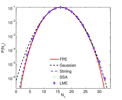
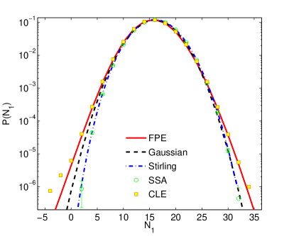
Figure 1: Empirical histograms of the probability distribution $P(N_{1})$ for the number of monomers $N_{1}$ obtained from the log-mean equation (left) and the chemical Langevin equation (right), compared to results from the CME (obtained using SSA). The theoretical solution of the corresponding FPE is shown with a solid red line; the numerical results from SSA are the circles. The Einstein distributions employing the Gaussian approximation and the second-order Stirling approximation (43) to the true entropy (40) are also shown. Note that $\langle N_{1}\rangle\approx 16$, which is rather small and thus tests the limits of applicability of a Langevin (non-discrete or non-integer) description.

Figure 1 shows numerical results for the equilibrium distribution of the number of monomers $N_{1}=n_{1}\Delta V=\rho Y_{1}\Delta V/m_{1}$. At thermal equilibrium the simulation results using the log-mean equation (LME) form for the noise are in excellent agreement with equilibrium statistical mechanics (see Appendix B) and with CME/SSA simulation results. Other work has also shown that, when detailed balance is obeyed, the LME correctly reproduces the equilibrium transition rates for rare jumps between stable minima in bistable systems Hanggi et al. (1984). On the other hand, the chemical Langevin equation (CLE) result has the noticeable flaw that, being a Gaussian, the distribution extends to unphysical negative values of $N_{1}$.

However, the LME does not compare favorably with the numerical solution of the CME for time-dependent situations, such as when a system is relaxing toward equilibrium. To illustrate this, we simulate an ensemble of systems prepared with an initial condition far from equilibrium, specifically with $Y_{1}(t=0)\approx 1$, and measure the time-dependent probability distribution $P(Y_{1},t)$ as the system relaxes toward chemical equilibrium ($(Y_{1})_{\mathrm{eq}}=\frac{1}{2}$). As expected, for the ensemble mean value of the number density $\bar{n}_{1}(t)=\langle n_{1}(t)\rangle$, we find close agreement among LME, CLE, and CME results (not shown), even when fluctuations are quite large. However, if we consider the standard deviation of the number of monomers, the left panel in Fig. 2 clearly demonstrates that the CLE is in much better agreement with the CME (as shown by the SSA results) for describing relaxation toward equilibrium. Also shown on this graph is the theoretical solution for the standard deviation obtained by first linearizing the CLE around the solution of the deterministic law of mass action (which is the law of large numbers corresponding to the CME Anderson and Kurtz (2011)), and then writing a system of ODEs for the mean and variance of $n_{1}(t)$. Specifically, we have that $d\bar{n}_{1}(t)/dt=\Omega_{1}$ and, using Ito’s formula, we get the central limit theorem corresponding to the CME Anderson and Kurtz (2011),

$$\frac{dC_{1}(t)}{dt}=-2C_{1}(t)\frac{d\Omega_{1}\left(\bar{n}_{1}(t)\right)}{dn_{1}}+\frac{8}{\Delta V}\mathcal{D}^{\mathrm{CL}}\left(\bar{n}_{1}(t)\right),$$

where $C_{1}(t)=\langle\left(n_{1}(t)-\bar{n}_{1}(t)\right)^{2}\rangle$.

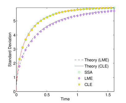
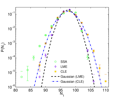
Figure 2: Relaxation toward equilibrium in a closed cell initially containing $100$ monomers and $4$ dimers and relaxing toward the equilibrium state of $\langle N_{1}\rangle\approx 54$ monomers. Rates are $k^{-}=0.3$ and $k^{+}=2.78\cdot 10^{-4}$; time step is $\Delta t=0.005$. (Left) Time evolution of the standard deviation of the number of monomers; theory curves are obtained by solving (IV.1.1). (Right) Histogram of the probability density $P(N_{1},\,t)$ for the number of monomers at an early time $t=0.05$.

The agreement between CLE and CME in the left panel of Fig. 2 is not surprising since it is well-known that the central limit theorem for the CME is a linear Langevin equation with the noise covariance given by the CLE form rather than the LME form. Ethier and Kurtz (2009); Anderson and Kurtz (2011) The agreement between the CLE and SSA results is less impressive when we look more closely at the probability distribution during the relaxation toward equilibrium. The right panel of Fig. 2 shows histograms of the probability distribution for the monomers, $P(N_{1},t)$, at an early time in the relaxation. This distribution is not close to Gaussian for the CME/SSA solution and we see that, in this regard, the CLE result is no better than the LME result. In fact, for the probability distribution of the dimers (not shown) the CLE results have the unphysical feature of non-zero probability for negative values of dimer concentration. Of course, one can argue that the number of molecules in the system is too small for a Langevin approximation to apply. If the fluctuations are decreased, the probability distribution $P(N_{1},t)$ will become closer to Gaussian and then the CLE will provide a better description; note however that the tails of the distribution will always be incorrect for the CLE, even at thermodynamic equilibrium.

IV.1.2 Bistable BPM Model

As a less trivial homogeneous example, we consider the BPM model (IV) for an open system held at a non-equilibrium steady state for which the probability distribution function is bimodal. Baras et al. (1996) For the chemistry-only study in this section, the number of molecules of species 1, 2, and 3 ($U$, $V$, and $W$) are allowed to vary while the number of molecules of all other species are fixed. The relevant parameters are given in Table 1. Note that a similar system (with all reactions being bimolecular) was studied by Baras et al., who found good agreement between SSA and molecular simulations using the Direct Simulation Monte Carlo (DSMC) algorithm  Baras et al. (1996). Baras et al. also examined the accuracy of the CLE linearized around the solution of the deterministic equations, and, not surprisingly, found it to be a very poor approximation of the CME for the parameters they chose. Gillespie Gillespie (2000) suggests that “A repetition of the study of Baras and co-workers using the Langevin equation [CLE] instead of the [linearized CLE] should show the chemical Langevin equation in a fairer light.” This section presents such a study using both the CLE and the LME. The parameters were selected such that the number of particles is large (roughly $O(10^{2}-10^{3})$ for each species) but not so plentiful as to prevent the SSA simulation from accurately sampling the bimodal distribution in a reasonable amount of computation time.

Species	$S$	$U_{f}$	$V_{f}$
$n_{r}$ (fixed)	$7.0\cdot 10^{2}$	$5\cdot 10^{11}$	$5.65\cdot 10^{10}$

-	$\mathfrak{R}_{1}$	$\mathfrak{R}_{2}$	$\mathfrak{R}_{3}$	$\mathfrak{R}_{4}$	$\mathfrak{R}_{5}$
$k^{+}$	$2\cdot 10^{-3}$	$10^{-3}$	0.0200936	0.28	0.28
$k^{-}$	$2\cdot 10^{-9}$	$2.198\cdot 10^{-4}$	$2.009\cdot 10^{-8}$	$2.8\cdot 10^{-10}$	$2.8\cdot 10^{-10}$

Table 1: Table of parameters for the BPM model in a well-mixed system (see Figure 3). The system volume $\Delta V=4$ and the time step $\Delta t=1.0$ (reducing the time step size further did not change the results significantly).

.

A phase-space picture of a typical trajectory is shown in the left panel of Fig. 3. The trajectory moves between two basins centered around the two stable deterministic steady states, which are labeled state $A$ (corresponding to $N_{1}\approx 1740,\,N_{2}\approx 448,\,N_{3}\approx 328$ molecules) and state $B$ (corresponds to $N_{1}\approx 1224,\,N_{2}\approx 936,\,N_{3}\approx 1424$ molecules). Based on this picture, we chose to define a collective coordinate $x(t)$ which is the projection of the state $(n_{1},n_{2},n_{3})$ onto the line connecting the two stable points (red line in the figure). This simple linear collective coordinate has the property that $x=0$ at state $A$ and $x=1$ at state $B$; note that $x(t)$ is not bounded between zero and one. The insert in Fig. 3 (left panel) shows $x(t)$ for a typical trajectory as the system moves between the basins.

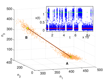
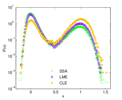
Figure 3: Numerical results for the BPM modelin a well-mixed system (see Table 1). (Left) A phase space picture of a typical trajectory from SSA as it visits the two basins around the deterministic steady states (labeled A and B in the figure). The insert shows the trajectory in the collective coordinate, $x(t)$, based on assigning each point to either state A (red) or state B (green) based on the last state visited by the trajectory (see text). (Right) Histogram of the steady-state probability distribution $P(x)$ comparing SSA, LME, and CLE simulation results. Measurements were skipped for the first $5\cdot 10^{5}$ steps to relax the initial transient and then statistics were collected for $1\cdot 10^{8}$ steps.

The right panel in Fig. 3 shows the steady-state probability distribution $P(x)$ for the collective coordinate $x$, clearly illustrating its bimodal form; similar results are found for the probability distributions for $n_{1}$, $n_{2}$, and $n_{3}$. The results for the LME and CLE Langevin approximations are qualitatively similar to those from the CME/SSA but quantitatively different; the LME result is in better agreement with the CME for this specific example. To also examine the long-time dynamics of the well-mixed bistable BPM system, we assign each (discrete) point in time to either state $A$ or state $B$ (see insert in left panel of Fig. 3). The assignment is performed by defining two sets $\mathcal{A}=\left\{x<0.3\right\}$ and $\mathcal{B}=\left\{x>0.6\right\}$ and assigning each point in the trajectory to the last set that was visited. The distribution of waiting times spent in the two states before transitioning to another state is related to the transition rate, and the ratio of the average waiting times gives the ratio of the probabilities to be found in each of the two states. For large $\Delta V$ (weak noise), the transitions are rare events and the distribution of waiting times should be approximately exponential (recall that for an exponential distribution the variance is the square of the mean). Numerical results for the mean and variance of the time spent in state B before transiting to state A, and vice versa, are shown in Table 2.

State A	Mean	Variance	State B	Mean	Variance
SSA	1.13$\cdot 10^{5}$	1.53$\cdot 10^{10}$	SSA	2.86$\cdot 10^{5}$	8.74$\cdot 10^{10}$
LME	3.23$\cdot 10^{5}$	9.03$\cdot 10^{10}$	LME	8.45$\cdot 10^{5}$	1.91$\cdot 10^{11}$
CLE	1.38$\cdot 10^{5}$	1.70$\cdot 10^{10}$	CLE	5.01$\cdot 10^{5}$	7.91$\cdot 10^{10}$

Table 2: Numerical results for the mean and variance of the time spent in state B before transiting to state A, and vice versa, for the three implementations of stochastic chemistry.

Our results indicate that for the BPM model the CLE and LME provide a reasonably good qualitative description of the long-time dynamics and rare-event statistics for the parameters studied here. However, both approximations are in general uncontrolled and the quantitative match between the CME and either CLE or LME will not improve even if the cell volume increases and the fluctuations decrease in amplitude. In Ref. Hanggi et al. (1984) it is observed that the LME correctly reproduces the very long-time dynamics (more precisely, the large deviation theory) of the CME for the bistable Schlogl model. This conclusion is, however, specific to this simple one-dimensional model because the system obeys detailed balance even though it is not in thermodynamic equilibrium; the BPM model studied here is not in detailed balance and there is no a priori reason to expect the LME to be more accurate than the CLE. The fact that the CLE is not able to describe rare events is well-known, see for example the discussion by Gillespie in Gillespie (2002) and after Eq. (9b) (which is the CLE) in Gillespie et al. (2013), or recent numerical studies of noise-induced multistability Duncan et al. (2014). It can, in fact, easily be proven that this problem is shared by all diffusion process (SODE) approximations of the CME , and fundamentally stems from the difference between the rare-event statistics of Gaussian and Poisson noise . A promising alternative is to use tau-leaping to approximately integrate the CME in time Gillespie et al. (2013) since it uses Poisson noise, and thus has the potential to correctly approximate the long-time behavior of the CME. This point is discussed further in the Conclusions.

IV.2 Giant Fluctuations

We now consider a system for which concentration fluctuations are affected by both chemistry and hydrodynamics in an interesting fashion. In the absence of chemistry a gradient of concentration induces a long-ranged correlation of concentration fluctuations Zarate and Sengers (2007); Donev et al. (2011a, b). These correlations are closely tied to the experimentally observed “giant fluctuation” phenomenon Segrè et al. (1993); Vailati and Giglio (1997); Vailati et al. (2011). In an isothermal, nonreacting binary mixture the static structure factor for fluctuations in the mass fraction of the first species contains two contributions,

$$S\left(k\right)=\left\langle(\widehat{\delta Y_{1}})(\widehat{\delta Y_{1}})^{\star}\right\rangle=S_{\text{eq}}+S_{\text{neq}},$$

where “hat” denotes a Fourier component; the equilibrium part is

$$S_{\text{eq}}=\frac{m_{1}}{\rho}(Y_{1})_{\text{eq}}\left(1-(Y_{1})_{\text{eq}}^{2}\right),$$ (28)

The non-equilibrium enhancement of the static structure factor due to a concentration gradient is $S_{\mathrm{neq}}\left(k\right)\sim\left(\nabla Y_{1}\right)^{2}/k^{4}$, where the wavevector $\bm{k}$ is perpendicular to the imposed concentration gradient.

The nature of these long-ranged correlations is modified in the presence of chemical reactions, as predicted by linearized fluctuating hydrodynamics  Lekkerkerker and Laidlaw (1974); de Zárate et al. (2007); Bedeaux et al. (2011). Some preliminary numerical studies of fluctuations in the presence of chemistry have been done in Ref. Hita and de Zárate (2013) using an RDME-based description. However, these simulations are for a simpler isomerization $A\rightleftarrows B$ in one dimension and, furthermore, they are concerned with reaction-diffusion only and do not account for the hydrodynamic velocity fluctuations that are responsible for the giant concentration fluctuation phenomenon.

We consider here the dimerization reaction (24) in a spatially inhomogeneous system. A rather detailed linearized fluctuating hydrodynamic theory for this example has been developed by Bedeaux et al. in Bedeaux et al. (2011), for a system in which a concentration gradient is imposed via a temperature gradient through the Soret effect. However, this analysis assumes a liquid mixture (large Schmidt and Lewis numbers) and thus does not apply to gas mixtures. Therefore, a simplified theoretical analysis of giant fluctuations in binary gas mixtures in the presence of an imposed constant concentration gradient and reactions is developed in Appendix C.

Our simplified theory decouples the temperature equation and uses a concentration equation (specifically the mass fraction of the first species) coupled to an incompressible fluctuating velocity equation. For the case of a liquid mixture with very large Schmidt number, which is the case considered in Bedeaux et al. (2011), the calculation predicts that the nonequilibrium enhancement of the static structure factor of concentration fluctuations for the monomer species is (see eqn. (44))

$$S_{\mathrm{neq}}\left(k\right)=\frac{k_{B}T\left(\nabla Y_{1}\right)^{2}}{\eta Dk^{4}}\,\left(1+\left(dk\right)^{-2}\right)^{-1},$$ (29)

where $D$ is the diffusion coefficient and $\eta$ is the viscosity. The last term on the r.h.s. depends on the penetration depth $d$ DeGroot and Mazur (1963),

$$d=\sqrt{\frac{D}{3k^{-}}}.$$

We see that for large wavenumbers ($k\gg 1/d$) the spectrum is $\sim k^{-4}$, as in the absence of the chemical reaction. However for small wavenumbers ($k\ll 1/d$) there is a transition to a $k^{-2}$ spectrum. For gas mixtures, however, a more detailed model is required that takes into account the finite value of the Schmidt number. The result of this calculation is eqn. (45), which predicts a further transition to a flat (constant) spectrum at small wavenumbers, with a finite $S_{\text{neq}}(k=0)=(k_{B}T)\left(\nabla Y_{1}\right)^{2}/(9\rho(k^{-})^{2})$. The calculation in Appendix C indicates that this effect is important even in liquids and the more refined theory ought to be used if quantitative agreement with experiments or simulations is sought.

We performed a series of simulations to investigate these predictions using the full hydrodynamic equations plus chemistry. It is important to note that even though we use the full nonlinear equations, nonlinearities in the fluctuations are negligible for the simulations reported here . In fact, the noise is very weak (since the domain is quite thick in the $z$ direction) and the numerical method is effectively performing a computational linearization of the fluctuating equations around the solution of the (nonlinear) deterministic equations Delong et al. (2014); this is simular to what is done analytically in Refs. de Zárate et al. (2007); Bedeaux et al. (2011) but does not require any approximations. In the small Gaussian noise regime the linearized CLE equation applies, and therefore in these simulations we use the CLE form for the stochastic chemical production rate in agreement with the theory in de Zárate et al. (2007); Bedeaux et al. (2011). Identical results (to within statistical errors) are obtained by using the LME form of the noise (not shown); this is not unexpected since the important noise here is the stochastic momentum tensor driving the velocity fluctuations; the stochastic mass flux and production rates only affect the reaction-diffusion part of the spectrum, which is much smaller than the nonequilibrium enhancement we study here.

Here we assume that the traditional number-density based LMA (20) holds with constant rates $k^{+}$ and $k^{-}$. This requires that the time scale for the reaction is proportional to the number density, that is, $\tau\sim p/k_{B}T=n$. From (18) and (19), for the dimerization of an ideal gas the ratio of these rates is,

$$\frac{k^{+}}{k^{-}}=\frac{(\Lambda_{1}^{3})^{2}}{\Lambda_{2}^{3}}\frac{j_{2}}{(j_{1})^{2}}=2^{3/2}\Lambda_{1}^{3}\frac{j_{2}}{(j_{1})^{2}}$$

which is a complicated function that depends on the form of the internal degrees of excitation. These details determine the number fraction $(X_{1})_{\mathrm{eq}}$ or, equivalently, the mass fraction $(Y_{1})_{\mathrm{eq}}$ at chemical equilibrium; here we set the ratio of the forward and reverse rates to ensure $(Y_{1})_{\mathrm{eq}}=1/2$, assuming that $\Lambda_{1}$, $j_{1}$ and $j_{2}$ are consistent with this choice. Since the reaction here changes the number density and thus the pressure, the reaction is strongly coupled to the momentum and energy transport equations. In order to minimize this coupling, we adjust the number of internal degrees of freedom of the dimer particles. Specifically, we set the heat capacities to $c_{p,1}=\frac{5}{2}k_{B}/m_{1}$ (corresponding to three translational and zero internal degrees of freedom), $c_{p,2}=5k_{B}/m_{2}$ (corresponding to three translational and five internal degrees of freedom). This choice ensures that $c_{p}$ of the mixture is independent of composition so that at constant pressure the reaction is isothermal.

The fluid was taken to be a dilute binary mixture of hard-sphere gases, using kinetic theory formulae for the transport coefficients Bell et al. (2010). In CGS units, the species diameters are $\sigma_{1}=2.58\cdot 10^{-8}$ and $\sigma_{2}=3.23\cdot 10^{-8}$, and $m_{1}=6.64\cdot 10^{-23}$. At equilibrium the density $\rho_{\mathrm{eq}}=1.78\cdot 10^{-3}$, the temperature $T_{\mathrm{eq}}=300$, and the concentration $(Y_{1})_{\mathrm{eq}}=0.5$. For these parameters, at the equilibrium conditions the mass diffusion coefficient is $D=0.2698$ while the momentum diffusion coefficient (kinematic viscosity) is $\nu=0.2374$. The ratio of the reverse and forward reaction rates is fixed at $k^{-}/k^{+}=\rho/m_{1}=2.67985\cdot 10^{19}$. We vary the penetration depth $d$ by changing the value of the reaction rates.

The simulations used a $128^{2}$ grid and time step size $\Delta t=2.5\cdot 10^{-8}$, grid spacing $\Delta x=\Delta y=10^{-3}$, and thickness in the $z$ direction of $\Delta z=10^{-3}$. The first $6\cdot 10^{4}$ time steps were skipped and then statistics collected for $2\cdot 10^{6}$ time steps. A steady concentration gradient was imposed by using Dirichlet boundary conditions at top and bottom boundaries ($y=L$ and $y=0$). Specifically, we take $Y_{1}\left(y=0,t\right)=0.3$ and $Y_{1}\left(y=L_{y},t\right)=0.7$, with temperature fixed at $T=300$ and no-slip boundary conditions for the velocity. Periodic boundary conditions were used in the other direction. Concentration profiles for various values of penetration depth, $d$, are shown in Fig. 4. As expected, when the chemistry is slow ($d\gg L$) the concentration profile is nearly linear; when the chemistry is fast the concentration is nearly constant (at its chemical equilibrium value of $(Y_{1})_{\mathrm{eq}}=1/2$) except near the boundaries. Note that we set the thermal diffusion ratio to zero (i.e., no Soret effect) so that the system is isothermal and the simple theory presented in Appendix C applies.

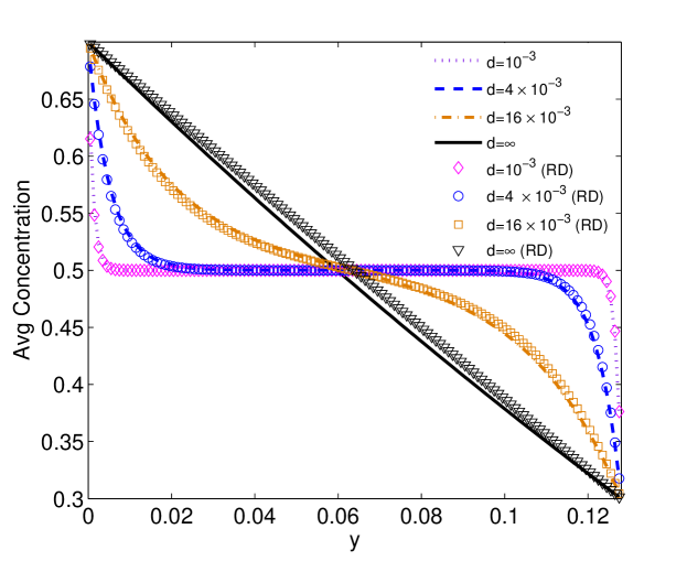
Figure 4: Average concentration profile $Y_{1}(y)$ at steady state for various values of penetration depth, $d$. Lines are from simulations using the full hydrodynamic equations; symbols are for reaction-diffusion only.

For comparison, we also performed simulations in which we turn off all hydrodynamics except Fickian diffusion, giving us a reference reaction-diffusion structure factor $S_{rd}(k)$. For the case of a binary mixture Bell et al. (2010) with $k^{-}/k^{+}=\rho/m_{1}$, the reaction-diffusion CLE reduces to

$$\frac{\partial}{\partial t}\left(Y_{1}\right) = \bm{\nabla}\cdot\left(D\bm{\nabla}Y_{1}\right)+k^{-}\left(-2Y_{1}^{2}+(1-Y_{1})\right)$$ (30)

$$+ \bm{\nabla}\cdot\left[\sqrt{\frac{2D}{n_{0}}Y_{1}(1-Y_{1}^{2})}\;\bm{\mathcal{Z}}^{\bm{\mathcal{F}}}\right]-\sqrt{\frac{2k^{-}}{n_{0}}\left(2Y_{1}^{2}+(1-Y_{1})\right)}\;\mathcal{Z}^{\Omega},$$ (31)

where $n_{0}=\rho_{1}/m_{1}+2\rho_{2}/m_{2}$ is the total number density of A particles contained in both monomers and dimers, which is spatially constant in this reaction-diffusion approximation. It is important to note that the reaction-diffusion model (31) is thermodynamically inconsistent because it ignores the coupling of the chemistry to the energy and momentum transport. It is well-known that adding chemistry should not change the fluctuations at thermodynamic equilibrium de Zárate et al. (2007), and this is indeed the case for the complete set of hydrodynamic equations that we study in this work. By contrast, for the reaction-diffusion (31) the equilibrium structure factor for $(Y_{1})_{\mathrm{eq}}=1/2$ is given by

$$S_{\text{eq}}^{(\text{rd})}=\frac{3m_{1}}{8\rho}\frac{8/9+k^{2}d^{2}}{1+k^{2}d^{2}},$$ (32)

which only approaches the thermodynamically correct answer (29) for $kd\gg 1$. Note that the inconsistency between full hydrodynamics and reaction-diffusion is not evident in Eqs. (27a,28) in de Zárate et al. (2007), because the authors of that work “neglect the dependence of the specific Gibbs energy difference on pressure.” This inconsistency is not of any importance in our study because we only use the reaction-diffusion simulations to obtain a baseline to subtract from the full hydrodynamic runs at large wavenumbers; at small wavenumbers the nonequilibrium enhancement is many orders of magnitude larger than the difference between (29) and (32).

The reaction-diffusion runs are not limited by the Courant condition so we increased the time step to $\Delta t=2.5\cdot 10^{-7}$; a total of $6\cdot 10^{4}$ steps were skipped initially and then statistics were collected for $3\cdot 10^{6}$ steps. As seen in Fig. 4 the average concentration profiles are nearly the same whether the simulations used the full hydrodynamic equations or simply species diffusion. For the structure factor, however, we find that the reaction-diffusion simulations do not reproduce the giant fluctuation result (29), rather, they follow (32), which does not show a power-law enhancement, as seen in the top panel of Fig. 5. This is expected since the giant fluctuation effect arises from the coupling of concentration fluctuations with the velocity fluctuations.

Because the equilibrium structure factor (28) is derived assuming a uniform bulk state, which is not actually the case here, we define $S_{\text{neq}}(k)=S(k)-S_{rd}(k)$ as a measure of the “giant” nonequilibrium fluctuations coming from the coupling with the velocity equation. Results for $S_{\text{neq}}(k)$ for several penetration depths are shown in the bottom panel of Fig. 5, comparing simulation results with the simple theory, eqn. (45). Since chemistry should have minimal effects for large $k$ according to the theory, we compute an effective concentration gradient by approximately matching the tail of the numerical result to the tail of the theory. We see that the theory correctly reproduces the qualitative trends, namely, that the giant fluctuations level off to a constant value at a wavenumber of order $d^{-1}$. However, except for the case of no reaction ($d\rightarrow\infty$), the theory is not in quantitative agreement with the simulations. To confirm that the issue is not under-resolution of the penetration depth by the grid, we perform runs with a finer grid of $256^{2}$ cells , and we get the same result over the common range of wavenumbers, showing these runs are sufficiently resolved for the purpose of computing $S(k)$. Note that in the plots the numerical wavenumber $k_{x}$ is corrected to account for discretization artifacts in the standard 5-point Laplacian, $k^{2}=\sin^{2}(k_{x}\Delta x/2)/(k_{x}\Delta x/2)^{2}$.

The mismatch between theory and simulation is not so surprising since the theory is for a weak gradient applied to a system that is essentially near equilibrium; this is not true in this setup. The only way to get this isothermal system out of equilibrium is via the boundaries, so the system is actually far from chemical equilibrium near the boundaries and then goes to chemical equilibrium in the middle of the domain, but in the middle the gradient disappears. A new more sophisticated theory is required that linearizes not around a constant state but rather around a spatially-dependent state (this is automatically done in our code). Also, boundaries (i.e., confinement effects) may need to be included, especially for penetration depths comparable to the system size.

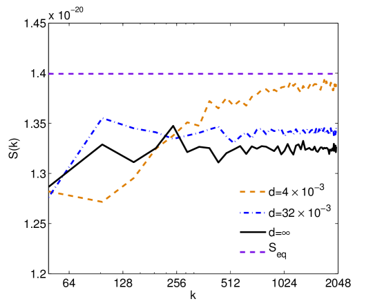
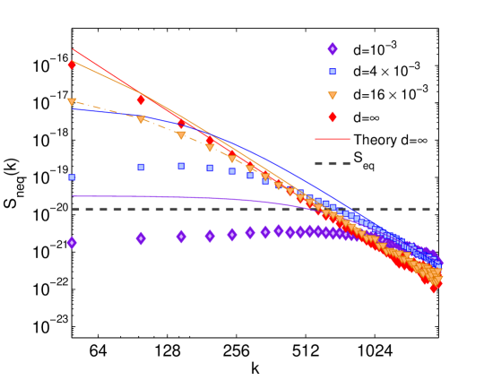
Figure 5: (Top) The structure factor $S_{rd}(k)$ for the reaction diffusion model (31) in the presence of an applied gradient. For small $d$ (fast reaction) the fact that the structure factor is not perfectly flat (constant) can be explained by (32) and comes from the thermodynamic inconsistency of the reaction-diffusion model. (Bottom) Non-equilibrium structure factors $S_{\text{neq}}(k)=S(k)-S_{rd}(k)$ for values of penetration depth $d$ varying from $\infty$ (no reaction) to $d=10^{-3}$, the width of one grid cell. Numerical results are shown with symbols, and the theoretical prediction (45) is shown as a line with the same color. In the absence of a gradient is flat, $S_{eq}\approx 1.4\cdot 10^{-20}$.

IV.3 Pattern Formation

Since the seminal work of Turing Turing (1952), pattern formation in deterministic reaction-diffusion systems has been investigated extensively, mostly in theoretical studies but also by laboratory experiments Kondo and Miura (2010); Cross and Greenside (2009). The study of stochastic systems is more recent and, as described in the introduction, has primarily focused on models based on a reaction-diffusion master equation (RDME). Such a model was introduced by Mansour and Houard Malek-Mansour and Houard (1979) as a practical numerical scheme for the study of correlations in spatially-distributed reactive systems. Subsequently RDME-based models have been used to study the influence of fluctuations on pattern formation for a variety of reaction-diffusion systems Lemarchand and Nowakowski (2011); Dziekan et al. (2013); Cao and Erban (2014); Zheng-Ping et al. (2008). Recently, a spatial chemical Langevin formulation (SCLE) was proposed Ghosh et al. (2015) and the RDME, SCLE and deterministic equations were compared for the development of patterns in the Gray-Scott model; it was observed that the SCLE is qualitatively similar to the RDME for the majority of examined sets of parameters, but not always. All of the RDME-based models usually use simplified descriptions of diffusion, but recently it has been observed that accounting for cross-diffusion effects (which are included in complete generality in our formulation) may lead to qualitatively-different behavior for Turing instabilities Biancalani et al. (2010); Fanelli et al. (2013); Kumar and Horsthemke (2011); Zemskov et al. (2013). Particle simulations including full hydrodynamics have also been performed using the DSMC method Dziekan et al. (2012) and molecular dynamics Dziekan et al. (2014); these are, however, limited to small systems in (quasi) one dimension because of the high computational cost of particle simulations.

In our final example we consider pattern formation in the Baras-Pearson-Mansour (BPM) model (IV) for a dilute gas mixture with full hydrodynamic transport. The system is initialized in a uniform constant “reference” state in which the number densities of the different species are as specified in Table 3. These number densities and the reaction rates are set so that the reference state is similar to that investigated in Baras et al. (1990). Specifically, under the assumption that the number densities of the reservoir or “solvent” species $S$, $U_{f}$, and $V_{f}$ are fixed, the deterministic dynamics of the three reactive species $U$, $V$, and $W$ starts close to the single unstable fixed point; the stable attractor of the dynamics is a limit cycle around this unstable point. Of course, when the number densities of the solvent species are not fixed the dynamics is six-dimensional and much more complex. Since we consider a time-dependent non-equilibrium scenario the chemical Langevin form of the noise (23) was used for the stochastic chemistry.

In the standard BPM model the solvent species ($S$, $U_{f}$, and $V_{f}$) have fixed concentrations but in our hydrodynamic simulations they were fixed only at the boundaries. These three species are also made abundant to buffer them from having rapid variations in concentration (see Table 3). In the limit of infinite concentrations of the solvent species ($S$, $U_{f}$, and $V_{f}$) the dynamics approaches a reaction-diffusion model in which advection as well as momentum and heat transport become negligible. The reference (initial) values for mole fraction are used to prescribe Dirichlet boundary conditions for species on each side of the domain. This setup mimics open reservoirs in the form of permeable membranes Donev et al. (2014a); note however that implementing boundaries that are also open for advective mass transport (i.e., inflow and outflow) is quite challenging Delgado-Buscalioni and Dejoan (2008) and not presently supported in our implementation. At the boundaries, the temperature is fixed at $T=300$K and the fluid velocity is set to zero (no-slip) so species transport is primarily due to mass diffusion.

In our hydrodynamic simulations the fluid is modeled as a hard sphere dilute gas so the transport coefficients depend on the masses and diameters of the particles of each species. The particles for all species in the BPM model have equal mass ($m=6.64\cdot 10^{-26}$ g) so as to ensure that the reactions conserve mass. For all species the particles have only translational energy and no internal degrees of freedom (i.e., $z=0$) so pressure and enthalpy are unaffected by reactions. In the BPM model species $U$ plays the role of the “inhibitor” while species $V$ is the “activator.” Cross and Greenside (2009) Typically pattern formation occurs when the inhibitor diffuses faster than the activator so we set the diameter of species $U$ particles to be smaller than that of $V$ particles, specifically $d_{1}=0.125$ nm and $d_{2}=0.5$ nm. Since we take $k_{1}^{+}\gg k_{1}^{-}$ (see Table 3), the intermediary species, $W$, supports the activation of $V$ and thus we set the diameters of $V$ and $W$ to be equal (this makes these two species hydrodynamically indistinguishable). The diameters of the other species ($S$, $U_{f}$, and $V_{f}$) are small, $d_{4}=d_{5}=d_{6}=0.025$ nm, so they diffuse rapidly from the boundaries and within the system. These specific values of the diameters are chosen such that the self-diffusion coefficient of $S$ (and $U_{f}$, $V_{f}$) is roughly an order of magnitude larger than the diffusion coefficient of $U$, which is itself an order of magnitude larger than the diffusion coefficient of $V$ (and $W$).

The system is simulated in a rectangular domain that is divided into $128\times 128\times 1$ cells with $\Delta x=\Delta y=100$ nm. The magnitude of the noise is varied by varying the domain thickness, which was either $\Delta z=100$ nm (low noise) or $10$ nm (high noise). The reference value for the number of molecules per cell for the species of interest, $U$, is $O(10^{4})$ in the former case and $O(10^{3})$ in the latter. The total number of solvent molecules per cell is $O(10^{6})$ for weak noise and $O(10^{5})$ for strong noise. The time step is $\Delta t=10$ ps, as determined from stability requirements for the explicit temporal integrator.

Figure 6 illustrates the pattern formation observed in the system for low noise (top row), high noise (middle row), and deterministic evolution (bottom row) started from a perturbed initial condition generated by the high noise simulation (see figure caption). The boundaries take some time to influence the center of the domain, so in the center the reservoir species are depleted and the system moves toward chemical equilibrium. However the boundary continuously forces the system so eventually spotted patterns develop, starting near the boundary, eventually filling the system. The resulting patterns are qualitatively similar to the “$\lambda$ pattern” observed by Pearson Pearson (1993) in the GS model. In simulations with only species diffusion (i.e., setting all other transport to zero) we find similar patterning, indicating that this system is well-approximated by reaction-diffusion due to very large solvent concentrations.

Reaction	$\mathcal{R}_{1}$	$\mathcal{R}_{2}$	$\mathcal{R}_{3}$	$\mathcal{R}_{4}$	$\mathcal{R}_{5}$
$k^{+}$	$2.0\cdot 10^{-11}$	$2.0\cdot 10^{-11}$	$3.3333\cdot 10^{9}$	$3.3333\cdot 10^{12}$	$3.3333\cdot 10^{12}$
$k^{-}$	$2.0\cdot 10^{-17}$	$2.0\cdot 10^{-12}$	$3.3333\cdot 10^{-1}$	$3.3333\cdot 10^{5}$	$3.3333\cdot 10^{5}$

Species	$U$	$V$	$W$	$S$	$U_{f}$	$V_{f}$
Boundary $n_{r}$	$1.513\cdot 10^{19}$	$4.38\cdot 10^{18}$	$3.8\cdot 10^{17}$	$5.0\cdot 10^{20}$	$1.33\cdot 10^{20}$	$5.0\cdot 10^{20}$

Table 3: Tables of reference number densities (bottom) and reaction rate parameters (top) for BPM model used to create Fig. 6, in CGS units.

In Turing (1952) Turing writes, “Another implicit assumption concerns random disturbing influences. Strictly speaking one should consider such influences to be continuously at work. This would make the mathematical treatment considerably more difficult without substantially altering the conclusions.” However, we see from Fig. 6 that the evolution is qualitatively different when large spontaneous fluctuations are present (middle row), as compared to when they are absent (bottom row). Specifically, the speed at which the patterns develop and propagate is noticeably accelerated by the spontaneous fluctuations (top and middle row), though the patterns themselves are qualitatively unchanged in this particular case. Other studies using reaction-diffusion models and particle simulations have reached similar conclusions Lemarchand and Nowakowski (2011); Dziekan et al. (2013); Cao and Erban (2014); Zheng-Ping et al. (2008). In Wang et al. (2007) the authors investigated the Gray-Scott model by RDME simulations and concluded, ’Complex spatiotemporal patterns, including spiral waves, Turing patterns, self-replicating spots and others, which are not captured or correctly predicted by the deterministic reaction-diffusion equations, are induced by internal reaction fluctuations.’

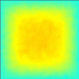
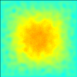
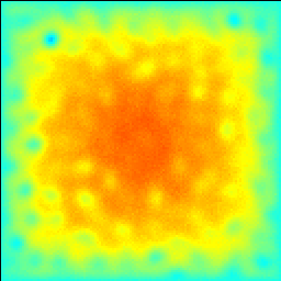
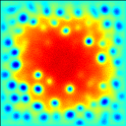
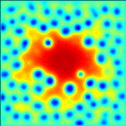
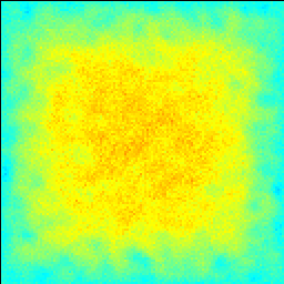
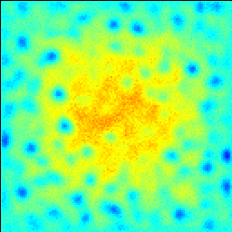
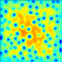
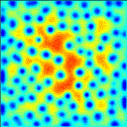
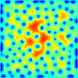
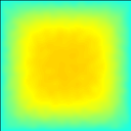
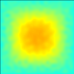
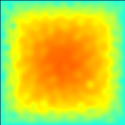
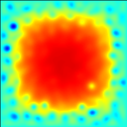
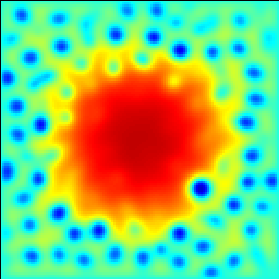
Figure 6: Time sequence of images of $\rho_{1}$ (species $U$) at $t=10$, 15, 20, 25, and 30 $\mu$s (time step $\Delta t=10$ ps, for other parameters see Table 3). The top row is a low noise case corresponding to a domain of thickness of $100$ nm; the middle row is a high noise case corresponding to a domain of thickness $10$ nm; and the bottom row is the deterministic evolution with an initial perturbation introduced by keeping high noise on up to time $t=2$ ns, and then turning the noise off. The color scale spans from $\rho_{1}=3.3\cdot 10^{-4}$ (blue) to $\rho_{1}=2.0\cdot 10^{-3}$ (red).

V Conclusions and Future Work

In this work we have formulated a fluctuating hydrodynamics model for chemically reactive ideal gas mixtures, and developed a numerical algorithm to solve the resulting system of stochastic partial differential equations. In our Langevin formalism, the stochastic mass, momentum and heat flux as well as the stochastic chemical production rate, are modeled using uncorrelated white noise processes, and the local number densities are real variables. This is contrast to the more traditional chemical master equation (CME) description of reactions that accounts for every individual reaction as a small jump of the (potentially very large) integer number of reactant molecules. We formulated the thermodynamic driving force for chemical reactions in agreement with nonlinear nonequilibrium thermodynamics Bedeaux et al. (2010) and considered two different Langevin formulations of the stochastic chemical production rate. The first formulation is based on the law of mass action cast in the GENERIC framework Öttinger and Grmela (1997) and leads to a noise covariance that is the logarithmic mean (LME) of the forward and reverse production rates. This formulation is fully consistent with equilibrium statistical mechanics, more specifically, the resulting dynamics is time reversible (i.e., satisfies detailed balance) with respect to the Einstein distribution for a closed system. The second formulation is based on the chemical Langevin equation (CLE) Gillespie (2000); Keizer (1987); Anderson and Kurtz (2011), and while it is not consistent with equilibrium statistical mechanics this form has its own merits.

We compared the two formulations on two chemical reaction networks for a well-mixed system, for both a simple dimerization reaction and a more complex network exhibiting bistability. We confirmed that at thermodynamic equilibrium the LME is more appropriate than the CLE, however, this is reversed for systems away from equilibrium, when compared with the CME. Not unexpectedly, neither is found to be entirely appropriate for describing rare events or large deviations from equilibrium. These examples remind us that a stochastic differential equation, which is a diffusion process, cannot be a uniformly accurate approximation for the CME, which is a Poisson process; the large-deviation statistics for Poisson noise is different than that of Gaussian noise. To further complicate the picture, there are known examples in which the discrete (integer-valued) nature of molecular populations plays a key role, implying that descriptions using real-valued concentrations such as fluctuating hydrodynamics must fail. For example, in wave fronts of the Fisher, Kolmogorov, Petrovski, Piskunov (FKPP) type it has been shown that the discreteness of the ME induces a logarithmic correction to the wave speed Hansen et al. (2006), similar to that observed when introducing a small cutoff in the leading edge of a FKPP front Brunet and Derrida (1997)

Another alternative coarse-grained description of stochastic chemistry, which we did not consider in this work, is tau leaping Gillespie et al. (2013); Hu et al. (2011); Anderson and Koyama (2012). Tau leaping is usually seen as a numerical method for approximately solving the CME, and the CLE can be seen as an approximation to tau leaping in a specific (central) limit in which a Poisson and a Gaussian variable become indistinguishable Gillespie et al. (2013); observe however that the two kinds of distributions always have different tails. A different and more interesting characterization of tau leaping is to see it instead as an alternative to the CLE that maintains the Poisson nature of the noise rather than replacing it with Gaussian noise. In the limit that the time step $\Delta t\rightarrow 0$, for Gaussian noise one gets the CLE, and for Poisson noise one gets, in principle, the CME. In this limit using the SSA algorithm is an efficient method to solve the CME exactly, and tau leaping is only useful as a numerical scheme for large $\Delta t$. As mentioned earlier, computational fluctuating hydrodynamics should only be considered useful (or even valid) when each update of the coarse-grained degrees of freedom involves an average over many molecular events, such as many molecular collisions for momentum and energy transport, or many reactive collisions for chemistry. In other words, to distinguish it from the CME and the associated SSA algorithm, for tau leaping one should choose the time step size in a way that ensures that many reactions occur in each reactive channel. In this sense, tau leaping can be seen as a coarse-graining in time of the CME jump process, and, when combined with spatial coarse-graining, has the potential to be a useful coarse-grained model that bypasses the need for Langevin models of chemistry in our numerical schemes for reactive fluctuating hydrodynamics. Additional studies are needed to access the accuracy of tau leaping in situations where Langevin descriptions do poorly and such investigations are in progress.

As is well-known, the failure of Langevin approximations to describe large deviations is in fact closely connected to the fact that traditional linear nonequilibrium thermodynamics fails to describe chemical reactions because the entropy production rate is generally a non-quadratic function of the thermodynamic driving force (affinity). The mesoscopic Kramers picture of chemical reactions, as developed for isomerization in Ref. Bedeaux et al. (2010), is an interesting approach, which, however, remains mostly of theoretical utility; numerical simulations of this model would need to handle additional dimensions, as well as very slow diffusion across the reaction barrier. Furthermore, it is not obvious how to extend this description to general multispecies fluids with complex reaction networks.

While the CME is a well-agreed upon and well-justified description of statistically homogeneous systems, the story is much less clear for systems with spatial inhomogeneity; in fact, the precise mathematical meaning of “well-mixed” and the range of validity of the RDME remains obscure. Fange et al. (2010); Hellander et al. (2015); Isaacson (2013) A law of large numbers has been rigorously proven for several particle models and takes the expected form of a deterministic reaction-diffusion partial differential equation. Arnold and Theodosopulu ; Arnold (1980) Regarding fluctuations, however, there are very few particle models for which central limit theorems Boldrighini et al. (1992) or large deviations functionals Jona-Lasinio et al. (1993) are known explicitly. It has been demonstrated that inhomogeneity leads to qualitative changes in the nature of phase transitions in bistable systems Tănase-Nicola and Lubensky (2012). It is also known that fluctuations can effectively renormalize the macroscopic transport and lead to non-analytic corrections to the law of mass action Kang and Redner (1984); Winkler and Frey (2012). It remains to be seen whether nonlinear spatially-extended fluctuating hydrodynamics models can correctly reproduce this effect compared to particle simulations.

Furthermore, most particle models used for reaction-diffusion problems assume independent random Brownian walkers that react when coming near each other, and thus completely neglect transport mechanisms such as advection, sound waves, thermal conduction, etc. Furthermore, the mechanism of diffusion used in these models implicitly neglects the long-ranged hydrodynamic correlations present among particles diffusing in a viscous solvent Donev and Vanden-Eijnden (2014). Notable exceptions are variants of the Direct Simulation Monte Carlo method (DSMC), which use a dilute Bird (1994); Alexander and Garcia (1997) or dense Donev et al. (2008) gas kinetic theory description of momentum and energy transport fully consistent with fluctuating hydrodynamics Donev et al. (2008). While chemical reactions are commonly included in DSMC schemes Goldsworthy et al. (2007); Lilley and Macrossan (2004), further studies of fluctuations and their consistency with nonequilibrium thermodynamics are needed. While some investigations of spatially-distributed reactive systems have been performed using DSMC Dziekan et al. (2012), a careful comparison to coarse-grained mesoscopic descriptions such as fluctuating hydrodynamics is needed. To model realistic chemistry modern DSMC codes use either the Total Collision Energy (TCE) model Bird (1994) or the more recent Quantum-Kinetic (QK) model Bird (2011), both of which we plan to compare with our formulations of reactive fluctuating hydrodynamics.

In Section IV.2 we studied the coupling of velocity fluctuations and chemistry in a system kept in a non-equilibrium steady state via boundary conditions. We found that, in agreement with existing theoretical computations, the chemical reactions have a strong effect on the giant long-range correlated concentration fluctuations. In this work we focused on gas mixtures, for which the Schmidt number is of order unity. We found that reactions profoundly change the nature of the giant fluctuations, whose spectrum switches from the well-known $\sim k^{-4}$ at large wavenumbers to a flat plateau (with a value controlled by the reaction rate) at small wavenumbers. This could be useful, for example, for experimentally measuring reaction rates. However, we found that the simple quasi-periodic near-equilibrium theory we constructed was not in quantitative agreement with the simulations, indicating that a more precise theory is needed.

Reactive liquid mixtures are common in practice and exhibit interesting coupling of hydrodynamics with transport that has been studied both theoretically Trevelyan et al. (2015) and experimentally Almarcha et al. (2013). The Schmidt number in liquids is, however, very large, and the compressibility is very small (i.e., the speed of sound is very large), making the method presented here computationally infeasible. In the future, we will consider extending low Mach number (quasi-incompressible) methods that treat momentum diffusion implicitly to include stochastic chemistry, by combining Langevin or tau-leaping based descriptions of chemistry with the formulation and numerical methods developed in Refs. Nonaka et al. (2015); Donev et al. (2015) for general non-ideal liquid mixtures.

Finally, the influence of hydrodynamic fluctuations on reactions will likely be very important for surface chemistry. Somorjai and Li (2010, 2011) An important application is heterogeneous catalysis in which a highly reactive catalytic surface facilitates bond breaking and bond rearrangement of adsorbed molecules. In this context mesoscale simulations are particularly useful for the study of nano-catalytic systems Moshfegh (2009). Microscopic catalytic particles have many advantages, such as higher activity, increased selectivity, and longer lifetime. However, to operate effectively these particles must have electrical contact with a substrate (typically a flat surface) and they must not be so small as to not have enough electrons to catalyze a reaction. For example, nanowire catalysts are typically 10-100 nm in size so the hydrodynamic environment in which the chemistry and transport occur is of mesoscopic scale (a few microns).

As in the case with chemistry in bulk flow, particle-based simulations will be useful benchmarks for comparison with reactive fluctuating hydrodynamics modeling surface chemistry. Furthermore, molecular simulations can be embedded within a fluctuating hydrodynamic code to create an Algorithm Refinement (AR) hybrid. Bell et al. (2010); Williams et al. (2008) The idea is to use a particle-based simulation for the domain near the surface to capture the physics at the molecular scale, such as adsorption of reactants onto the surface, surface diffusion, surface reactions, and desorption of products. This particle-based simulation would then be coupled to a fluctuating hydrodynamic simulation that treats the bulk fluid. Previous work for non-reactive fluids has already proven the utility of AR hybrids for simple interfaces Donev et al. (2010c) and this numerical framework should prove useful in the study of surface reactions and active membrane transport.

Appendix A Deterministic and Stochastic Transport in Ideal Gas Mixtures

This appendix summarizes fluctuating hydrodynamics for ideal gas mixtures; for a more general and detailed exposition see Balakrishnan et al. (2014). Each of the hydrodynamic transport terms in (1)-(3) contains a deterministic term, denoted with an overbar and a stochastic term denoted by a tilde (e.g., ${\bm{\mathcal{F}}}=\overline{\bm{\mathcal{F}}}+\widetilde{\bm{\mathcal{F}}}$). The deterministic viscous tensor is,

$$\overline{\bm{\Pi}}=-\eta\left(\nabla\mathbf{v}+(\nabla\mathbf{v})^{T}\right)-\left(\kappa-\frac{2}{3}\eta\right)\mathbf{I}\left({\bf\nabla}\cdot{\bf v}\right),$$ (33)

where $\eta$ and $\kappa$ are the shear and bulk viscosity, respectively. We neglect any possible effect of the chemical reactions on the transport coefficients of the mixture. For example, we neglect any coupling between bulk viscosity and chemical reactions, which, in principle is allowed by the Curie principle since both are scalar processes. Grossmann (1976) The corresponding stochastic viscous flux tensor can be written as Landau and Lifshitz (1959); Español (1998)

$$\widetilde{\bm{\Pi}}(\mathbf{r},t)=\sqrt{2k_{B}T\eta}\;\widehat{\mathcal{Z}}^{\bm{\Pi}}+\left(\sqrt{\frac{k_{B}\kappa T}{3}}-\sqrt{\frac{2k_{B}\eta T}{3}}\right)\text{Tr}(\widehat{\mathcal{Z}}^{\bm{\Pi}}).$$ (34)

The symmetric Gaussian random tensor field, $\widehat{\mathcal{Z}}^{\bm{\Pi}}$, is formulated as $\widehat{\mathcal{Z}}^{\bm{\Pi}}=\left(\mathcal{Z}^{\bm{\Pi}}+(\mathcal{Z}^{\bm{\Pi}})^{T}\right)/\sqrt{2}$ where $\mathcal{Z}^{\bm{\Pi}}$ is a white-noise random Gaussian tensor field, that is, $\langle\mathcal{Z}^{\bm{\Pi}}\rangle=0$ and,

$$\langle\mathcal{Z}^{\bm{\Pi}}_{\alpha\beta}(\mathbf{r},t)\mathcal{Z}^{\bm{\Pi}}_{\gamma\delta}(\mathbf{r}^{\prime},t^{\prime})\rangle=\delta_{\alpha\gamma}\delta_{\beta\delta}\,\delta(\mathbf{r}-\mathbf{r}^{\prime})\,\delta(t-t^{\prime})\;\;.$$

with $\alpha,\beta,\gamma,\delta=\{x,y,z\}$ being spatial components.

The deterministic mass flux and heat flux depend on the gradients of concentration, pressure, and temperature. For an ideal gas we can write the deterministic fluxes as

$$\bm{\mathcal{F}} = -\rho\mathcal{Y}\mathbf{D}\left(\mathbf{d}+\mathcal{X}\tilde{\chi}\frac{\nabla T}{T}\right)\qquad\mathrm{and}$$ (35)

$$\bm{\mathcal{Q}} = -\lambda\nabla T+(k_{B}T\tilde{\chi}^{T}\mathcal{M}^{-1}+h^{T})\bm{\mathcal{F}}$$ (36)

where $h$ is a vector of specific enthalpies. Here the diffusion driving force Kuiken (1994) is

$$\mathbf{d}={\nabla}X+\left(X-Y\right)\frac{{\nabla}p}{p}.$$

and $\cal{X}$, $\cal{Y}$ and $\cal{M}$ are diagonal matrices of mole fractions $X$, mass fractions $Y$ and molecular masses $M$. The matrix of multicomponent flux diffusion coefficients, $\mathbf{D}$, the vector of rescaled thermal diffusion ratios, $\tilde{\chi}$, and the thermal conductivity, $\lambda$, can be obtained from standard software libraries, such as EGLIB Ern and Giovangigli (2004), or from standard references, such as Hirshfelder et al. Hirschfelder et al. (1967).

For the ideal gas transport coefficients described above, we define

$${\mathbf{L}}=\frac{\rho\overline{m}}{k_{B}}\mathcal{Y}\mathbf{D}\mathcal{Y},\qquad{\xi}=k_{B}T\mathcal{M}^{-1}\tilde{\chi},\qquad\zeta=T^{2}{\lambda}.$$ (37)

where $\overline{m}=(\sum_{s}Y_{s}/m_{s})^{-1}$ is the mixture-averaged molecular mass. The stochastic terms for the combined species equations and energy equation are determined from the phenomenological equations of nonequilibrium thermodynamics that relate fluxes to thermodynamic driving forces through the Onsager matrix, and the fluctuation-dissipation balance principle. Balakrishnan et al. (2014) Specifically, the stochastic mass flux is

$$\widetilde{\bm{\mathcal{F}}}=\mathbf{B}\;\bm{\mathcal{Z}}^{\bm{\mathcal{F}}}$$ (38)

where $\mathbf{B}\mathbf{B}^{T}=2k_{b}\mathbf{L}$, and $\bm{\mathcal{Z}}^{\bm{\mathcal{F}}}$ is a white-noise random Gaussian vector field with uncorrelated components, that is, $\langle\bm{\mathcal{Z}}^{\bm{\mathcal{F}}}\rangle=0$ and

$$\langle{\mathcal{Z}}^{\bm{\mathcal{F}}}_{\alpha s}(\mathbf{r},t){\mathcal{Z}}^{\bm{\mathcal{F}}}_{\beta s^{\prime}}(\mathbf{r}^{\prime},t^{\prime})\rangle=\delta_{\alpha\beta}\delta_{s,s^{\prime}}\,\delta(\mathbf{r}-\mathbf{r}^{\prime})\,\delta(t-t^{\prime})$$

with $\alpha,\beta=\{x,y,z\}$ being spatial components. Note that the matrix $\mathbf{B}$ can be obtained using Cholesky decomposition; the constraint $\sum_{s}\widetilde{\bm{\mathcal{F}}}_{s}=0$ is ensured by construction. Balakrishnan et al. (2014) The stochastic heat flux is

$$\widetilde{\bm{\mathcal{Q}}}=\sqrt{\zeta}\bm{\mathcal{Z}}^{\bm{\mathcal{Q}}}+(\xi^{T}+h^{T})\widetilde{\bm{\mathcal{F}}},$$ (39)

where $\langle{\mathcal{Z}}^{\bm{\mathcal{Q}}}_{\alpha}(\mathbf{r},t){\mathcal{Z}}^{\bm{\mathcal{Q}}}_{\beta}(\mathbf{r}^{\prime},t^{\prime})\rangle=\delta_{\alpha\beta}\,\delta(\mathbf{r}-\mathbf{r}^{\prime})\,\delta(t-t^{\prime})$.

Appendix B Equilibrium distribution for a dimerization reaction

The entropy of mixing for a system undergoing dimerization is $S=k_{B}\ln N_{p}$, where $N_{p}$ is the number of distinct ways of forming $M$ dimers out of a total of $N$ monomers. This is straightforward to compute. The number of ways to choose $2M$ out of the $N$ atoms to be in pairs is,

$$\left(\begin{array}[]{c}N\\ 2M\end{array}\right)=\frac{N!}{\left(2M\right)!\left(N-2M\right)!}$$

Next we need to group the $2M$ atoms into pairs; the number of distinct ways of pairing $2M$ objects is ${(2M)!}/{2^{M}M!}.$ This gives the entropy

$$S=k_{B}\ln\left(\frac{N!}{2^{M}M!\left(N-2M\right)!}\right)+k_{B}\mu M,$$ (40)

where we have included an additional reference chemical potential $\mu$ to set the equilibrium concentration.

By expanding the logarithm of the right-hand side of (40) using Stirling’s leading-order approximation we obtain the thermodynamic limit of the entropy as a function of the monomer mass fraction $Y_{1}=\left(N-2M\right)/N$. After fixing the chemical potential from the requirement that the most probable mass fraction is $(Y_{1})_{\text{eq}}=1/2$, we get,

$$S=Nk_{B}\left[-\frac{1}{2}\,\ln\left(1-Y_{1}\right)\left(1-Y_{1}\right)-Y_{1}\ln\left(Y_{1}\right)-\frac{1}{2}\,Y_{1}\left(\ln\left(2\right)-1\right)\right],$$ (41)

This gives an Einstein distribution $P\sim e^{S/k_{B}}$ exactly matching (27).

It is useful to compare this equilibrium distribution of the LME with that of the CME for a well-mixed system of volume $\Delta V$. It is not hard to show that the CME for a dimerization reaction is in detailed balance with respect to the Einstein distribution with entropy (40), with the reference chemical potential set to

$$\mu=\ln\left(\frac{2k^{+}}{\Delta V\,k^{-}}\right).$$ (42)

We can use this to construct a rather accurate continuum approximation to this exact microscopic result by including the next order term in the Stirling formula,

$$N!\approx\sqrt{2\pi N}\left(\frac{N}{e}\right)^{N},$$ (43)

when expanding (40). This gives a better continuous approximation (labeled “Stirling” in the figures in the main body of this paper) to the discrete Einstein distribution than (41), especially for small number of particles in the well-mixed cell.

Appendix C Giant fluctuations in the presence of reactions

This appendix outlines the fluctuating hydrodynamics theory for the long-range correlations of concentration fluctuations in a binary mixture undergoing a dimerization reaction, as studied numerically in Section IV.2. We neglect the Dufour effect and assume the system to be isothermal, taking contributions from temperature fluctuations to be of higher order. Furthermore, we neglect gravity, assume the system is incompressible, and take the density and transport coefficients to be constant. We consider a “bulk” system Zarate and Sengers (2007), i.e., we neglect the influence of the boundaries. This gives an accurate approximation for wavenumbers that are large compared to the inverse height of the domain; for smaller wavenumbers the boundaries are expected to suppress the giant fluctuations Zarate and Sengers (2007); Ortiz de Zarate et al. (2006). We also neglect the stochastic mass flux in the concentration equation since we are concerned with the nonequilibrium contribution due to the forcing by the velocity fluctuations.

We assume that all of the concentration gradients are in the same direction (say, the $y$ axis). The incompressibility constraint is most easily handled by applying a $\bm{\nabla}\times\bm{\nabla}\times$ operator to the momentum equation  Zarate and Sengers (2007) to obtain a system involving only the component of the velocity parallel to the gradient, $v_{\parallel}\equiv v_{y}$. The same calculation can easily be generalized to a multispecies mixture as well, see Appendix B in Ref. Balakrishnan et al. (2014). This system of equations can be most easily solved in the Fourier domain, by considering wavevectors $\bm{k}$ in the plane perpendicular to the gradient, $\bm{k}=\bm{k}_{\perp}$.

It is very straightforward to derive (29) in the limit of large Schmidt number by considering the fluctuating concentration equation forced by an overdamped (steady Stokes) fluctuating velocity. The steady Stokes equation in Fourier space has the form,

$$\eta k^{2}\hat{v}_{\parallel}=\sqrt{2\eta k_{B}T_{0}}\;ik\widehat{\mathcal{W}}(t),$$

where $T_{0}$ is the constant temperature. Here $\widehat{\mathcal{W}}(t)$ is a white-noise process (one per wavenumber), giving the white-in-time velocity $\hat{v}_{\parallel}(t)=k^{-1}\sqrt{2k_{B}T_{0}/\eta}\;i\widehat{\mathcal{W}}(t)$. A general form of the linearized equation for the concentration fluctuations, $c=\delta Y_{1}=Y_{1}-\left\langle Y_{1}\right\rangle$, in Fourier space will have the form

$$\partial_{t}\hat{c}=-Dk^{2}\hat{c}-\psi\hat{c}-\hat{v}_{\parallel}f=-\left(Dk^{2}+\psi\right)\hat{c}-if\sqrt{\frac{2k_{B}T_{0}}{\eta k^{2}}}\widehat{\mathcal{W}}(t),$$

where $\psi$ is the reaction rate at the equilibrium point (around which we are linearizing), and $f=d\left\langle Y_{1}\right\rangle/dy$ is the applied concentration gradient. For our specific reaction and the choice of equilibrium point $(Y_{1})_{\text{eq}}=1/2$, we have that $\psi=3k^{-}$ (to see this simply linearize (31) around $(Y_{1})_{\text{eq}}=1/2$). The resulting nonequilibrium static structure factor (recall that here we neglect the contribution due to the stochastic mass flux) is straightforward to calculate (see, for example, Appendix B in Ref. Balakrishnan et al. (2014)),

$$S_{\text{neq}}(k)=\left\langle\hat{c}\hat{c}^{\star}\right\rangle=\frac{k_{B}T_{0}}{\eta k^{2}\left(Dk^{2}+\psi\right)}f^{2}=\frac{k_{B}T_{0}}{\eta Dk^{4}\left(1+\psi D^{-1}k^{-2}\right)}f^{2},$$ (44)

which is exactly (29) with the penetration depth

$$d^{2}=\frac{D}{\psi}=\frac{D}{3k^{-}}.$$

Since the Schmidt number is not very large for gases, we should improve the theory by not taking the overdamped limit but rather adding a velocity equation and considering the linearized inertial equations,

$$\partial_{t}\hat{c} = -Dk^{2}\hat{c}-\psi\hat{c}-\hat{v}_{\parallel}f$$

$$\rho_{0}\partial_{t}\hat{v}_{\parallel} = -\eta k^{2}\hat{v}_{\parallel}+\sqrt{2\eta k_{B}T_{0}}\;ik\widehat{\mathcal{W}}(t),$$

where $\rho_{0}$ is the equilibrium density and $\nu=\eta/\rho_{0}$ is the kinematic viscosity. Solving this system of linear SODEs gives the improved structure factor

$$S_{\text{neq}}(k)=\frac{k_{B}T_{0}}{\eta Dk^{4}\left(1+\psi D^{-1}k^{-2}\right)\left(\frac{D+\nu}{\nu}+\psi\nu^{-1}k^{-2}\right)}f^{2},$$ (45)

which shows that the finite value of the Schmidt number $S_{c}=\nu/D$ has an important effect on the giant fluctuations. In particular, in the more complete theory (45)

$$S_{\text{neq}}(k=0)=\frac{k_{B}T_{0}}{\rho_{0}\psi^{2}}f^{2}$$

is finite and not infinite as in (44), which assumes infinite Schmidt number.

In the more complete theory we see the following three regimes:

1. For large wavenumbers we have

   $$S_{\text{neq}}\left(k\gg\sqrt{\frac{D}{\psi}}\right)\approx\frac{k_{B}T_{0}}{\eta Dk^{4}}f^{2}$$

   as if there were no reaction.

2. If the Schmidt number is small, $D\sim\nu$, as for gases, then for small wavenumbers we instantly switch to a flat spectrum

   $$S_{\text{neq}}\left(k\ll\sqrt{\frac{D}{\psi}}\right)\approx\frac{k_{B}T_{0}}{\rho_{0}\psi^{2}}f^{2}$$

3. If the Schmidt number $S_{c}$ is large, $D\ll\nu$, as for liquids, then for intermediate wavenumbers

   $$S_{\text{neq}}\left(\sqrt{\frac{D}{\psi}}\ll k\ll S_{c}^{\frac{1}{2}}\sqrt{\frac{D}{\psi}}\right)\approx\frac{k_{B}T_{0}}{\eta\psi k^{2}}f^{2}$$

   we observe a change in the power law to $S_{\text{neq}}(k)\sim k^{-2}$. Note however that this range spans only $\sqrt{S_{c}}$ orders of magnitude in $k$, so even for $S_{c}\sim 10^{4}$ (which applies to macromolecular solutions), the $k^{-2}$ power-law only extends over at most two decades. Therefore, even for liquids with large Schmidt numbers the inertial equations should be used to model giant fluctuations in reactive mixtures.

References

- Lemarchand and Nowakowski (2004) A. Lemarchand and B. Nowakowski, Molecular Simulation 30, 773 (2004).
- Kang and Redner (1984) K. Kang and S. Redner, Phys. Rev. Lett. 52, 955 (1984).
- Winkler and Frey (2012) A. A. Winkler and E. Frey, Phys. Rev. Lett. 108, 108301 (2012).
- Lemarchand and Nowakowski (2011) A. Lemarchand and B. Nowakowski, EPL (Europhysics Letters) 94, 48004 (2011).
- Dziekan et al. (2013) P. Dziekan, L. Signon, B. Nowakowski, and A. Lemarchand, The Journal of chemical physics 139, 114107 (2013).
- Cao and Erban (2014) Y. Cao and R. Erban, Bulletin of mathematical biology 76, 3051 (2014).
- Zheng-Ping et al. (2008) F. Zheng-Ping, X. Xin-Hang, W. Hong-Li, and O. Qi, Chinese Physics Letters 25, 1220 (2008).
- Dziekan et al. (2014) P. Dziekan, J. S. Hansen, and B. Nowakowski, The Journal of Chemical Physics 141, 124106 (2014).
- Almarcha et al. (2013) C. Almarcha, P. M. Trevelyan, P. Grosfils, and A. De Wit, Physical Review E 88, 033009 (2013).
- Brogioli (2010) D. Brogioli, Phys. Rev. Lett. 105, 058102 (2010).
- Brogioli (2011) D. Brogioli, Phys. Rev. E 84, 031931 (2011).
- Brogioli (2013) D. Brogioli, The Journal of Chemical Physics 139, 184102 (2013).
- Mahmutovic et al. (2012) A. Mahmutovic, D. Fange, O. G. Berg, and J. Elf, Nature methods 9, 1163 1166 (2012).
- Malek-Mansour and Nicolis (1975) M. Malek-Mansour and G. Nicolis, Journal of Statistical Physics 13, 197 (1975).
- Nicolis and Prigogine (1977) G. Nicolis and I. Prigogine, Self-organization in nonequilibrium systems: from dissipative structures to order through fluctuations, A Wiley-Interscience Publication (Wiley, 1977).
- Gardiner (2003) C. W. Gardiner, Handbook of stochastic methods: for physics, chemistry & the natural sciences, 3rd ed., Series in synergetics, Vol. Vol. 13 (Springer, 2003).
- Erban et al. (2007) R. Erban, J. Chapman, and P. Maini, arXiv preprint arXiv:0704.1908 (2007).
- Fange et al. (2012) D. Fange, A. Mahmutovic, and J. Elf, Bioinformatics 28, 3155 (2012), http://bioinformatics.oxfordjournals.org/content/28/23/3155.full.pdf+html .
- Gillespie (1976) D. T. Gillespie, Journal of Computational Physics 22, 403 (1976).
- Gillespie (2007) D. T. Gillespie, Annual Review of Physical Chemistry 58, 35 (2007).
- Fange et al. (2010) D. Fange, O. G. Berg, P. Sjöberg, and J. Elf, Proceedings of the National Academy of Sciences 107, 19820 (2010).
- Hellander et al. (2015) S. Hellander, A. Hellander, and L. Petzold, Phys. Rev. E 91, 023312 (2015).
- Isaacson (2013) S. A. Isaacson, The Journal of Chemical Physics 139, 054101 (2013).
- Dobrzynski et al. (2007) M. Dobrzynski, J. V. Rodr guez, J. A. Kaandorp, and J. G. Blom, Bioinformatics 23, 1969 (2007), http://bioinformatics.oxfordjournals.org/content/23/15/1969.full.pdf+html .
- Andrews et al. (2010) S. S. Andrews, N. J. Addy, R. Brent, and A. P. Arkin, PLoS Comput Biol 6, e1000705 (2010).
- van Zon and ten Wolde (2005a) J. S. van Zon and P. R. ten Wolde, Phys. Rev. Lett. 94, 128103 (2005a).
- van Zon and ten Wolde (2005b) J. S. van Zon and P. R. ten Wolde, J. Chem. Phys. 123, 234910 (2005b).
- Oppelstrup et al. (2009) T. Oppelstrup, V. V. Bulatov, A. Donev, M. H. Kalos, G. H. Gilmer, and B. Sadigh, Phys. Rev. E 80, 066701 (2009).
- Donev et al. (2010a) A. Donev, V. V. Bulatov, T. Oppelstrup, G. H. Gilmer, B. Sadigh, and M. H. Kalos, J. Comp. Phys. 229, 3214 (2010a).
- Mauro et al. (2014) A. J. Mauro, J. K. Sigurdsson, J. Shrake, P. J. Atzberger, and S. A. Isaacson, J. Comp. Phys. 259, 536 (2014).
- Bezzola et al. (2014) A. Bezzola, B. B. Bales, R. C. Alkire, and L. R. Petzold, J. Comp. Phys. 256, 183 (2014).
- Gillespie et al. (2014) D. T. Gillespie, E. Seitaridou, and C. A. Gillespie, The Journal of Chemical Physics 141, 234115 (2014).
- Kuo (2005) K. Kuo, Principle of Combustion (John Wiley & Sons, 2005).
- Law (2006) C. Law, Combustion Physics (Cambridge University Press, 2006).
- Zarate and Sengers (2007) J. M. O. D. Zarate and J. V. Sengers, Hydrodynamic fluctuations in fluids and fluid mixtures (Elsevier Science Ltd, 2007).
- Landau and Lifshitz (1959) L. Landau and E. Lifshitz, Fluid Mechanics, Course of Theoretical Physics, Vol. 6 (Pergamon Press, Oxford, England, 1959).
- Garcia et al. (1987) A. Garcia, M. Malek-Mansour, G. Lie, M. Mareschal, and E. Clementi, Phys. Rev. A 36, 4348 (1987).
- Adhikari et al. (2005) R. Adhikari, K. Stratford, M. E. Cates, and A. J. Wagner, Europhysics Letters 71, 473 (2005), arXiv:cond-mat/0402598 .
- Bell et al. (2010) J. Bell, A. Garcia, and S. Williams, ESAIM: M2AN 44, 1085 (2010).
- Donev et al. (2010b) A. Donev, E. Vanden-Eijnden, A. L. Garcia, and J. B. Bell, Communications in Applied Mathematics and Computational Science 5, 149 (2010b).
- Shang et al. (2012) B. Shang, N. Voulgarakis, and J. Chu, J. Chem. Phys. 137, 044117 (2012).
- Balakrishnan et al. (2014) K. Balakrishnan, A. L. Garcia, A. Donev, and J. B. Bell, Phys. Rev. E 89, 013017 (2014).
- Donev et al. (2014a) A. Donev, A. J. Nonaka, Y. Sun, T. G. Fai, A. L. Garcia, and J. B. Bell, Communications in Applied Mathematics and Computational Science 9, 47 (2014a).
- Donev et al. (2015) A. Donev, A. J. Nonaka, A. K. Bhattacharjee, A. L. Garcia, and J. B. Bell, “Low Mach Number Fluctuating Hydrodynamics of Multispecies Liquid Mixtures,” (2015), to appear in Physics of Fluids, ArXiv:1412.6503.
- Koh and Blackwell (2012) W. Koh and K. T. Blackwell, The Journal of Chemical Physics 137, 154111 (2012), http://dx.doi.org/10.1063/1.4758459.
- Ghosh et al. (2015) A. Ghosh, A. Leier, and T. T. Marquez-Lago, Theoretical Biology and Medical Modelling 12, 5 (2015).
- Gillespie (2000) D. T. Gillespie, The Journal of Chemical Physics 113, 297 (2000).
- Segrè et al. (1993) P. N. Segrè, R. W. Gammon, and J. V. Sengers, Phys. Rev. E 47, 1026 (1993).
- Vailati and Giglio (1997) A. Vailati and M. Giglio, Nature 390, 262 (1997).
- Vailati et al. (2011) A. Vailati, R. Cerbino, S. Mazzoni, C. J. Takacs, D. S. Cannell, and M. Giglio, Nature Communications 2, 290 (2011).
- Donev et al. (2014b) A. Donev, T. G. Fai, and E. Vanden-Eijnden, Journal of Statistical Mechanics: Theory and Experiment 2014, P04004 (2014b).
- Donev and Vanden-Eijnden (2014) A. Donev and E. Vanden-Eijnden, J. Chem. Phys. 140, 234115 (2014), http://dx.doi.org/10.1063/1.4883520.
- Donev et al. (2010c) A. Donev, J. B. Bell, A. L. Garcia, and B. J. Alder, SIAM J. Multiscale Modeling and Simulation 8, 871 (2010c).
- Franz et al. (2013) B. Franz, M. B. Flegg, S. J. Chapman, and R. Erban, SIAM Journal on Applied Mathematics 73, 1224 (2013).
- Haken (2004) H. Haken, Synergetics: Introduction and Advanced Topics, Physics and Astronomy Online Library (Springer, 2004).
- Atzberger (2010) P. J. Atzberger, J. Comp. Phys. 229, 3474 (2010).
- Keizer (1987) J. Keizer, Statistical thermodynamics of nonequilibrium processes (Springer, 1987).
- Pagonabarraga et al. (1997) I. Pagonabarraga, A. Pérez-Madrid, and J. Rubi, Physica A: Statistical Mechanics and its Applications 237, 205 (1997).
- Bedeaux et al. (2010) D. Bedeaux, I. Pagonabarraga, J. de Zárate, J. Sengers, and S. Kjelstrup, Phys. Chem. Chem. Phys. 12, 12780 (2010).
- de Zárate et al. (2007) J. de Zárate, J. Sengers, D. Bedeaux, and S. Kjelstrup, J. Chem. Phys. 127, 034501 (2007).
- Bedeaux et al. (2011) D. Bedeaux, J. O. de Zárate, I. Pagonabarraga, J. Sengers, and S. Kjelstrup, J. Chem. Phys. 135, 124516 (2011).
- Öttinger and Grmela (1997) H. Öttinger and M. Grmela, Physical Review E 56, 6633 (1997).
- Español et al. (2009) P. Español, J. Anero, and I. Zúñiga, J. Chem. Phys. 131, 244117 (2009).
- de la Torre et al. (2015) J. de la Torre, P. Espa ol, and A. Donev, 142, 094115 (2015), http://dx.doi.org/10.1063/1.4913746.
- Grima et al. (2011) R. Grima, P. Thomas, and A. V. Straube, The Journal of chemical physics 135, 084103 (2011).
- Gillespie et al. (2013) D. Gillespie, A. Hellander, and L. Petzold, J. Chem. Phys. 138 (2013).
- Grabert et al. (1983) H. Grabert, P. Hänggi, and I. Oppenheim, Physica A: Statistical Mechanics and its Applications 117, 300 (1983).
- Hanggi et al. (1984) P. Hanggi, H. Grabert, P. Talkner, and H. Thomas, Phys. Rev. A 29, 371 (1984).
- Anderson and Kurtz (2011) D. F. Anderson and T. G. Kurtz, in Design and analysis of biomolecular circuits (Springer, 2011) pp. 3–42.
- Baras et al. (1990) F. Baras, J. E. Pearson, and M. M. Mansour, The Journal of Chemical Physics 93, 5747 (1990).
- Baras et al. (1996) F. Baras, M. M. Mansour, and J. E. Pearson, The Journal of Chemical Physics 105, 8257 (1996).
- (72) L. Arnold and M. Theodosopulu, Advances in Applied Probability 12, pp. 367.
- Arnold (1980) L. Arnold, in Dynamics of synergetic systems (Springer, 1980) pp. 107–118.
- Grossmann (1976) S. Grossmann, The Journal of Chemical Physics 65, 2007 (1976).
- Ottinger (2015) H. C. Ottinger, (2015), draft.
- Bedeaux et al. (2014) D. Bedeaux, S. Kjelstrup, and H. C. Öttinger, The Journal of chemical physics 141, 124102 (2014).
- Bedeaux and Kjelstrup (2008) D. Bedeaux and S. Kjelstrup, Physical Chemistry Chemical Physics 10, 7304 (2008).
- Öttinger (2005) H. C. Öttinger, Beyond equilibrium thermodynamics (Wiley Online Library, 2005).
- Klimontovich (1994) Y. L. Klimontovich, Physics-Uspekhi 37, 737 (1994).
- Hütter and Öttinger (1998) M. Hütter and H. Öttinger, J. Chem. Soc., Faraday Trans. 94, 1403 (1998).
- Grabert (1982) H. Grabert, Projection operator techniques in nonequilibrium statistical mechanics (Springer-Verlag, 1982).
- Kjelstrup et al. (2010) S. Kjelstrup, D. Bedeaux, E. Johannessen, and J. Gross, Non-Equilibrium Thermodynamics for Engineers (World Scientific Pub Co Inc, 2010).
- Kuiken (1994) G. D. C. Kuiken, Thermodynamics of Irreversible Processes: Applications to Diffusion and Rheology (Wiley, 1994).
- Kondepudi and Prigogine (1998) D. Kondepudi and I. Prigogine, Modern thermodynamics: from heat engines to dissipative structures (John Wiley, 1998).
- Zemansky and Dittman (1981) M. Zemansky and R. Dittman, Heat and Thermodynamics: An Intermediate Textbook, International student edition: MacGraw-Hill (McGraw-Hill, 1981).
- Pathria and Beale (2011) R. Pathria and P. Beale, Statistical Mechanics (Elsevier Science, 2011).
- Giovangigli (1999) V. Giovangigli, Multicomponent Flow Modeling (Birkhauser Boston, 1999).
- Mielke (2013) A. Mielke, Calculus of Variations and Partial Differential Equations 48, 1 (2013).
- Mielke (2011) A. Mielke, Nonlinearity 24, 1329 (2011).
- Delong et al. (2013) S. Delong, B. E. Griffith, E. Vanden-Eijnden, and A. Donev, Phys. Rev. E 87, 033302 (2013).
- Delong et al. (2014) S. Delong, Y. Sun, , B. E. Griffith, E. Vanden-Eijnden, and A. Donev, Phys. Rev. E 90, 063312 (2014).
- Usabiaga et al. (2012) F. B. Usabiaga, J. B. Bell, R. Delgado-Buscalioni, A. Donev, T. G. Fai, B. E. Griffith, and C. S. Peskin, SIAM J. Multiscale Modeling and Simulation 10, 1369 (2012).
- Kloeden and Platen (2010) P. Kloeden and E. Platen, Numerical Solution of Stochastic Differential Equations, Stochastic Modelling and Applied Probability (Springer Berlin Heidelberg, 2010).
- Öttinger (2012) H. Öttinger, Stochastic Processes in Polymeric Fluids: Tools and Examples for Developing Simulation Algorithms (Springer Berlin Heidelberg, 2012).
- Anderson and Mattingly (2011) D. Anderson and J. Mattingly, Communications in Mathematical Sciences 9, 301 (2011).
- Gray and Scott (1983) P. Gray and S. Scott, Chemical Engineering Science 38, 29 (1983).
- Gray and Scott (1985) P. Gray and S. K. Scott, The Journal of Physical Chemistry 89, 22 (1985).
- Pearson (1993) J. E. Pearson, 261, 189 (1993).
- van Kampen (2007) N. G. van Kampen, Stochastic Processes in Physics and Chemistry, 3rd ed. (Elsevier, 2007).
- Ethier and Kurtz (2009) S. N. Ethier and T. G. Kurtz, Markov processes: characterization and convergence, Vol. 282 (John Wiley & Sons, 2009).
- Gillespie (2002) D. T. Gillespie, The Journal of Physical Chemistry A 106, 5063 (2002).
- Duncan et al. (2014) A. Duncan, S. Liao, T. Vejchodsky, R. Erban, and R. Grima, arXiv preprint arXiv:1407.8256 (2014).
- Heymann and Vanden-Eijnden (2008) M. Heymann and E. Vanden-Eijnden, Communications on pure and applied mathematics 61, 1052 (2008).
- Donev et al. (2011a) A. Donev, A. L. Garcia, A. de la Fuente, and J. B. Bell, Phys. Rev. Lett. 106, 204501 (2011a).
- Donev et al. (2011b) A. Donev, A. L. Garcia, A. de la Fuente, and J. B. Bell, J. of Statistical Mechanics: Theory and Experiment 2011, P06014 (2011b).
- Lekkerkerker and Laidlaw (1974) H. N. W. Lekkerkerker and W. G. Laidlaw, Phys. Rev. A 9, 346 (1974).
- Hita and de Zárate (2013) J. L. Hita and J. M. O. de Zárate, Physical Review E 87, 052802 (2013).
- DeGroot and Mazur (1963) S. R. DeGroot and P. Mazur, Non-Equilibrium Thermodynamics (North-Holland Publishing Company, Amsterdam, 1963).
- Ortiz de Zarate et al. (2006) J. M. Ortiz de Zarate, J. A. Fornes, and J. V. Sengers, Phys. Rev. E 74, 046305 (2006).
- Turing (1952) A. M. Turing, Philosophical Transactions of the Royal Society of London B: Biological Sciences 237, 37 (1952).
- Kondo and Miura (2010) S. Kondo and T. Miura, 329, 1616 (2010).
- Cross and Greenside (2009) M. Cross and H. Greenside, Pattern Formation and Dynamics in Nonequilibrium Systems (Cambridge University Press, 2009).
- Malek-Mansour and Houard (1979) M. Malek-Mansour and J. Houard, Physics Letters A 70, 366 (1979).
- Biancalani et al. (2010) T. Biancalani, D. Fanelli, and F. Di Patti, Phys. Rev. E 81, 046215 (2010).
- Fanelli et al. (2013) D. Fanelli, C. Cianci, and F. Di Patti, The European Physical Journal B 86, 1 (2013).
- Kumar and Horsthemke (2011) N. Kumar and W. Horsthemke, Phys. Rev. E 83, 036105 (2011).
- Zemskov et al. (2013) E. P. Zemskov, K. Kassner, M. J. B. Hauser, and W. Horsthemke, Phys. Rev. E 87, 032906 (2013).
- Dziekan et al. (2012) P. Dziekan, A. Lemarchand, and B. Nowakowski, The Journal of Chemical Physics 137, 074107 (2012).
- Delgado-Buscalioni and Dejoan (2008) R. Delgado-Buscalioni and A. Dejoan, Phys. Rev. E 78, 046708 (2008).
- Wang et al. (2007) H. Wang, Z. Fu, X. Xu, and Q. Ouyang, The Journal of Physical Chemistry A 111, 1265 (2007).
- Hansen et al. (2006) J. S. Hansen, B. Nowakowski, and A. Lemarchand, The Journal of Chemical Physics 124, 034503 (2006).
- Brunet and Derrida (1997) E. Brunet and B. Derrida, Phys. Rev. E 56, 2597 (1997).
- Hu et al. (2011) Y. Hu, T. Li, and B. Min, J. Chem. Phys. 135, 024113 (2011).
- Anderson and Koyama (2012) D. F. Anderson and M. Koyama, Multiscale Modeling & Simulation 10, 1493 (2012).
- Boldrighini et al. (1992) C. Boldrighini, A. De Masi, and A. Pellegrinotti, Stochastic processes and their applications 42, 1 (1992).
- Jona-Lasinio et al. (1993) G. Jona-Lasinio, C. Landim, and M. Vares, Probability theory and related fields 97, 339 (1993).
- Tănase-Nicola and Lubensky (2012) S. Tănase-Nicola and D. K. Lubensky, Physical Review E 86, 040103 (2012).
- Bird (1994) G. Bird, Molecular Gas Dynamics and the Direct Simulation of Gas Flows (Clarendon, Oxford, 1994).
- Alexander and Garcia (1997) F. J. Alexander and A. L. Garcia, Computers in Physics 11, 588 (1997).
- Donev et al. (2008) A. Donev, A. L. Garcia, and B. J. Alder, Phys. Rev. Lett 101, 075902 (2008).
- Goldsworthy et al. (2007) M. J. Goldsworthy, M. N. Macrossan, and M. M. Abdel-Jawad, Physics of Fluids 19, 066101 (2007).
- Lilley and Macrossan (2004) C. Lilley and M. Macrossan, Physics of Fluids 16, 2054 (2004).
- Bird (2011) G. A. Bird, Physics of Fluids (1994-present) 23, 106101 (2011).
- Trevelyan et al. (2015) P. M. J. Trevelyan, C. Almarcha, and A. De Wit, Phys. Rev. E 91, 023001 (2015).
- Nonaka et al. (2015) A. J. Nonaka, Y. Sun, J. B. Bell, and A. Donev, “Low Mach Number Fluctuating Hydrodynamics of Binary Liquid Mixtures,” (2015), submitted to CAMCOS, ArXiv preprint 1410.2300.
- Somorjai and Li (2010) G. Somorjai and Y. Li, Introduction to Surface Chemistry and Catalysis (John Wiley & Sons, 2010).
- Somorjai and Li (2011) G. A. Somorjai and Y. Li, Proceedings of the National Academy of Sciences 108, 917 (2011).
- Moshfegh (2009) A. Z. Moshfegh, Journal of Physics D: Applied Physics 42, 233001 (2009).
- Williams et al. (2008) S. A. Williams, J. B. Bell, and A. L. Garcia, SIAM J. Multiscale Modeling and Simulation 6, 1256 (2008).
- Español (1998) P. Español, Physica A 248, 77 (1998).
- Ern and Giovangigli (2004) A. Ern and V. Giovangigli, EGLIB: A general-purpose Fortran library for multicomponent transport property evaluation, Version 3.4 (2004).
- Hirschfelder et al. (1967) J. Hirschfelder, C. Curtiss, and R. Bird, Molecular Theory of Gases and Liquids, Structure of matter series (Wiley, 1967).