Search for Sterile Neutrinos in Muon Neutrino Disappearance Mode at FNAL

Abstract

The NESSiE Collaboration has been setup to undertake a conclusive experiment to clarify the muon–neutrino disappearance measurements at short baselines in order to put severe constraints to models with more than the three–standard neutrinos. To this aim the current FNAL–Booster neutrino beam for a Short–Baseline experiment was carefully evaluated by considering the use of magnetic spectrometers at two sites, near and far ones. The detector locations were studied, together with the achievable performances of two OPERA–like spectrometers. The study was constrained by the availability of existing hardware and a time–schedule compatible with the undergoing project of multi–site Liquid–Argon detectors at FNAL.
The settled physics case and the kind of proposed experiment on the Booster neutrino beam would definitively clarify the existing tension between the $\nu_{\mu}$ disappearance and the $\nu_{e}$ appearance/disappearance at the eV mass scale. In the context of neutrino oscillations the measurement of $\nu_{\mu}$ disappearance is a robust and fast approach to either reject or discover new neutrino states at the eV mass scale. We discuss an experimental program able to extend by more than one order of magnitude (for neutrino disappearance) and by almost one order of magnitude (for antineutrino disappearance) the present range of sensitivity for the mixing angle between standard and sterile neutrinos. These extensions are larger than those achieved in any other proposal presented so far.

1 Introduction and Physics Overview

The unfolding of the physics of the neutrino is a long and pivotal history spanning the last 80 years. Over this period the interplay of theoretical hypotheses and experimental facts was one of the most fruitful for the progress in particle physics. The achievements of the last decade and a half brought out a coherent picture within the Standard Model (SM) or some minor extensions of it, namely the mixing of three neutrino flavour–states with three $\nu_{1}$, $\nu_{2}$ and $\nu_{3}$ mass eigenstates. Few years ago a non-vanishing $\theta_{13}$, the last still unknown mixing angle, was measured theta13 . Once the absolute masses of neutrinos, their Majorana/Dirac nature and the existence and magnitude of leptonic CP violation be determined, the (standard) three–neutrino model will be beautifully settled. Still, other questions would remain open: the reason for the characteristic nature of neutrinos, the relation between the leptonic and hadronic sectors of the SM, the origin of Dark Matter and, overall, where and how to look for Beyond Standard Model (BSM) physics. Neutrinos may be an excellent source of BSM physics and their history supports that possibility at length.

There are indeed several experimental hints for deviations from the “coherent” neutrino oscillation picture recalled above. Many unexpected results, not corresponding to a discovery on a single basis, accumulated in the last decade and a half, bringing attention to the hypothesis of the existence of sterile neutrinos pontecorvo . A White Paper whitepaper provides a comprehensive review of these issues. In particular tensions in several phenomenological models grew up with experimental results on neutrino/antineutrino oscillations at Short–Baseline (SBL) and with the more recent, recomputed antineutrino–fluxes from nuclear reactors.

The main source of tension originates from the absence so far of any $\nu_{\mu}$ disappearance signal kopp-tension . Limited experimental data are available on searches for $\nu_{\mu}$ disappearance at SBL: the rather old CDHS experiment CDHS and the more recent results from MiniBooNE mini-mu , a joint MiniBooNE/SciBooNE analysis mini-sci-mu and the MINOS recent-MINOS and SuperKamiokande recent-SK exclusion limits reported at the NEUTRINO2014 conference. The tension between $\nu_{e}$ appearance and $\nu_{\mu}$ disappearance was actually strengthened by the MINOS and SuperKamiokande results, even if they only slightly extend the $\nu_{\mu}$ disappearance exclusion region set previously mainly by CDHS and at higher mass scale by the CCFR experiment ccfr . Fig. 1 shows the excluded regions in the parameter space that describe SBL $\nu_{\mu}$ disappearance induced by a sterile neutrino. The mixing angle is denoted as $\theta_{new}$ and the squared mass difference as $\Delta m^{2}_{new}$. As evident from Fig. 1, the region $\sin^{2}(2\theta_{new})<0.1$ is still largely unconstrained. While this paper was being processed by the referees of the Journal new results were made available. In particular a joint analysis by MINOS and DAYA-BAY new-ster-1 , and the IceCube experiment new-ster-2 . Their results exclude part of the phase space $\sin^{2}(2\theta_{new})<0.1$ even if the critical region $\Delta m^{2}_{new}\sim 1$ eV² is still only marginally touched, while the $\nu_{\mu}$– $\nu_{e}$ tension from global–fits stays around 0.04–0.07 for $\sin^{2}(2\theta_{new})$ kopp-tension . For $\overline{\nu}_{\mu}$ the situation is even worse as it will be further discussed in Section 6.

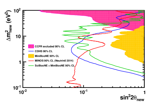
Figure 1: (color online) The current exclusion limits on the $\nu_{\mu}$ disappearance searches at the eV² scale. Blue (green) line: old (recent) exclusion limits on $\nu_{\mu}$ from previous CDHS CDHS and recent MiniBooNE/SciBooNE mini-sci-mu measurements. The two filled areas correspond to the exclusion limits on the $\overline{\nu}_{\mu}$ from CCFR ccfr and MiniBooNE–alone mini-mu experiments. The red curve corresponds to the very recent result from MINOS recent-MINOS . All the exclusion limits were compute at 90% C.L..

The outlined scenario promoted several proposals for new, exhaustive evaluations of the neutrino phenomenology at SBL. Since the end of 2012 CERN started the setting up of a Neutrino Platform edms , with new infrastructures at the North Area that, for the time being, does not include a neutrino beam. Meanwhile in the US, FNAL welcomed proposals for experiments exploiting the physics potentials of their two existing neutrino beams, the Booster and the NuMI beams, following the recommendations from USA HEP–P5 report p5 . Two proposals ICARUSFNAL ; LAr1-ND were submitted for SBL experiments at the Booster beam, to complement the about to start MicroBooNE experiment microboone . They are all based on the Liquid–Argon (LAr) technology and aim to measure the $\nu_{e}$ appearance at SBL, with less possibilities to investigate the $\nu_{\mu}$ disappearance SBN . In this paper a complementary case study based on magnetic spectrometers at two different sites at FNAL–Booster beam is discussed, built up on the following considerations:

1. the measurement of $\nu_{\mu}$ spectrum in both normalization and shape is mandatory for a correct interpretation of the $\nu_{e}$ data, even in case of a null result for the latter;

2. a decoupled measurement of $\nu_{e}$ and $\nu_{\mu}$ interactions allows to reach in the analyses the percent–level systematics due to the different cross–sections;

3. very massive detectors are mandatory to collect a large number of events thus improving the disentangling of systematic effects.

This paper is organized in the following way. After the introduction a short overview of the NESSiE proposal is given. A detailed report of the studies performed on the constraints of the FNAL–Booster neutrino beam is drawn in Section 3. In Section 4 a description of the detector system and the corresponding outcomes are provided. The statistical analyses and the attainable exclusion-limits on the $\nu_{\mu}$ and $\overline{\nu}_{\mu}$ disappearances are depicted in Sections 5 and 6, respectively. Finally conclusions are drawn.

2 Proposal for the FNAL–Booster beam

Assuming the use of the FNAL–Booster neutrino beam a detailed study of the physics case was performed along the lines followed when considering neutrino beams at CERN–PS and CERN–SPS nessie ; larnessie and the approach of the analysis reported in stancoetal . A substantial difference between FNAL and CERN beams is the decrease of the average neutrino energy by more than a factor 2, thus making the study very challenging for an high Z–density detector. Several detector configurations were studied, investigating experimental aspects not fully addressed by the LAr detection, such as the measurements of the lepton charge on event–by–event basis and the lepton energy over a wide range. Indeed, muons from Charged Current (CC) neutrino interactions play an important role in disentangling different phenomenological scenarios provided their charge state is determined. Also, the study of muon appearance/disappearance can benefit from the large statistics of CC events from the primary muon neutrino beam.

In the FNAL–Booster neutrino beam the antineutrino contribution is rather small and it corresponds to a systematic effect to be taken into account. For the antineutrino beam the situation is rather different since a large flux of neutrinos is also present. From an experimental perspective the possibility of an event–by–event detection of the primary muon charge is an added value since it allows to disentangle the presence/absence of new effects which might genuinely affect antineutrinos and neutrinos differently (CP violation is possible in models with more than one additional sterile neutrino). This possibility is particularly intriguing while running in negative horn polarity due to the sizable contamination from the cross-section enhanced interactions of parasitic neutrinos.

The extended NESSiE proposal is available in nessie-fnal . It consists in the design, construction and installation of two spectrometers at two sites, Near (at 110 m, on–axis) and Far (at 710 m, off-axis, on surface), in line with the FNAL–Booster beam and compatible with the proposed LAr detectors. Profiting of the large mass of the two spectrometer–systems, their performances as stand–alone apparatus are exploited for the $\nu_{\mu}$ disappearance study. Besides, complementary measurements with the foreseen LAr–systems can be undertaken to increase their control of systematic errors.

Practical constraints were assumed in order to draft a proposal on a conservative, manageable basis, with sustainable timescale and cost–wise. Well known technologies were considered as well as re–using of large parts of existing detectors.

The momentum and charge state measurements of muons in a wide range, from few hundreds MeV/c to several GeV/c, over a $>\ 50\ {\rm m}^{2}$ surface, are an extremely challenging task. In the following, the key features of the proposed experimental layout are presented. By keeping the systematic error at the level of $1-2$% for the detection of the $\nu_{\mu}$ interactions, it will be possible to:

• measure the $\nu_{\mu}$ disappearance in a large muon–momentum, $p_{\mu}$, range (conservatively a $p_{\mu}\geq 500$ MeV/c cut is chosen) in order to reject existing anomalies over the whole expected parameter space of sterile neutrino oscillations at SBL;

• collect a very large statistical sample so as to test the hypothesis of muon (anti)neutrino disappearance for values of the mixing parameter down to still un–explored regions ($\sin^{2}(2\theta_{new})\lesssim 0.01$);

• measure the neutrino flux at the near detector, in the relevant muon momentum range, in order to keep the systematic errors at the lowest possible values;

• measure the sign of the muon charge to separate $\nu_{\mu}$ from $\overline{\nu}_{\mu}$ for the control of the systematic error.

3 Beam evaluation and constraints

For a proposal that aims to make measurements with the FNAL–Booster muon–neutrino beam the convolution of the beam features and of the muon detection constitutes the major constraint. An extended study was therefore performed.

3.1 The Booster Neutrino Beam (BNB)

The neutrino beam G4BNBflux is produced from protons with a kinetic energy of 8 GeV extracted from the Booster and directed to a Beryllium cylindrical target 71 cm long and with a 1 cm diameter. The target is surrounded by a magnetic focusing horn pulsed with a 170 kA current at a rate of 5 Hz. Secondary mesons are projected into a 50 m long decay–pipe where they are allowed to decay in flight before being stopped by an absorber and the ground material. An additional absorber could be placed in the decay pipe at about 25 m from the target. This configuration, not currently in use, would modify the beam properties providing a more point–like source at the near site and thus extra experimental constraints on the systematic errors.

Neutrinos travel about horizontally at a depth of 7 m underground. Proton batches from the Booster contain $\sim 4.5\times 10^{12}$ protons, have a duration of 1.6 $\mu$s and are subdivided into 84 bunches. Bunches are $\sim 4$ ns wide and are separated by 19 ns. The rate of batch extraction is limited by the horn pulsing at 5 Hz. This timing structure provides a very powerful constraint to the background from cosmic rays.

3.2 The Far–to–Near Ratio (FNR)

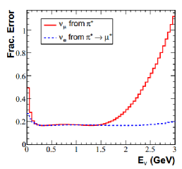
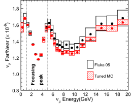
Figure 2: (color online) Top: uncertainties on the absolute flux of $\nu_{\mu}$ at MiniBooNE (from G4BNBflux ). Bottom: uncertainties on the far–to–near ratio at NuMI according to different simulations (from numikopp ).

The uncertainty on the absolute $\nu_{\mu}$ flux at MiniBooNE, shown in Fig. 2, top (from G4BNBflux ), stays below 20% for energies below 1.5 GeV, increasing drastically at larger energies and also below 200 MeV. The uncertainty is dominated by the knowledge of proton interactions in the Be target, which affects the angular and momentum spectra of neutrino parents. The result of Fig. 2 is based on experimental data obtained by the HARP and E910 collaborations G4BNBflux .

The large uncertainty on the absolute neutrino flux makes the use of two or more identical detectors at different baselines mandatory when searching for small disappearance phenomena. The ratio of the event rates at the far and near detectors (FNR) as function of neutrino energy is a convenient variable since at first order it benefits from cancellation of systematics due to the common effects of proton–target, neutrino cross–sections and reconstruction efficiencies. Because of these cancellations the uncertainty on the FNR or, equivalently, on the spectrum at the far site extrapolated from the spectrum at the near site is at the level of few percent. As an example the FNR for the NuMI beam is shown in bins of neutrino energy in Fig. 2, bottom (from numikopp ); the uncertainty ranges in the interval 0.5–5.0%.

It is worth to note that, even in the absence of oscillations, the energy spectra in any two detectors are different, thus leading to a non–flat FNR. This is especially true if the distance of the near detector is comparable with the length of the decay pipe. It is therefore necessary to master the knowledge of the FNR for physics searches.

Assuming a transverse area for the detectors at near and far sites of the same order, the solid angle subtended by the near detector is larger than that subtended by the far one. Therefore, neutrinos, and mostly those from mesons decaying at the end of the pipe, have a higher probability of being detected in the near than in the far detector. In the far detector, on the contrary, only neutrinos produced in a narrow forward cone are visible. This effect is illustrated in Fig. 3 showing the ratio of the integrated neutrino flux at the two locations distributed over the neutrino production points (radius $R$ vs longitudinal coordinate $Z$), for a sample crossing a near ($4\times 4$ m² transverse area) and a far ($8\times 8$ m²) detector with front–surface placed at 110 and 710 m from the target, respectively. Neutrinos produced at large $Z$ can be detected even if they are produced at relatively large angles, enhancing the contribution of lower energy neutrinos. On the other hand neutrinos from late decays come from the fast pion component that is more forward–boosted. The former effect is the leading one so the net effect is a softer spectrum at the near site.

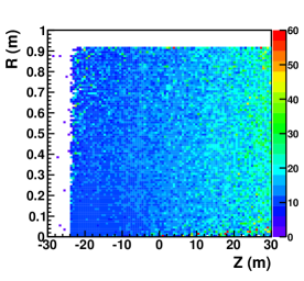
Figure 3: (color online) Ratio between the $Z$–$R$ distributions of neutrino production points for neutrinos crossing a near–detector transverse surface of $4\times 4$ m² at 110  m over neutrinos crossing a far–detector transverse surface of $8\times 8$ m² at 710  m. The $Z$ origin is fixed at the middle of the decay pipe, $R$ being the radial distance in the pipe. The near detector has a larger acceptance for neutrinos produced in the most downstream part of the decay pipe, as expected.

In Fig. 4 (top plots) the distributions of the neutrino energy, $E_{\nu}$, vs $Z$ for neutrinos crossing the near (top left) and the far site (top right) are shown. The assumed detector active surface is a square of $4\times 4$ m² and $8\times 8$ m² for the near and far detector, respectively. As anticipated, the energy spectrum at the near site is softer, the additional contribution at low energy being particularly important for neutrinos from late meson–decays. The distribution of $Z$ is also shown in Fig. 4 for neutrinos crossing the detectors at the near (bottom left) and far (bottom right) sites.

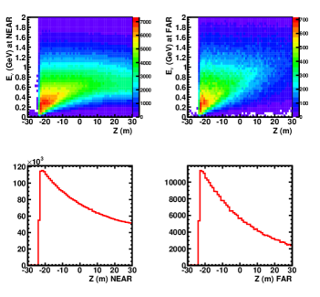
Figure 4: (color online) Distribution of $E_{\nu}$ vs $Z$ for neutrinos seen in the near (top left) and far (top right) detector. Distribution of the $Z$ production points for neutrinos seen in the near (bottom left) and far (bottom right) detectors. The assumed detector active surface is a square of $4\times 4$ m² and $8\times 8$ m² for the near and far detector, respectively.

From these considerations it is apparent that the prediction of the FNR is a delicate task requiring the full simulation of the neutrino beam–line and the detector acceptance. Moreover, the systematic uncertainties on the FNR parameter play a major role requiring deep investigation.

The various contributions to the systematic uncertainties on the neutrino flux were studied in detail by the MiniBooNE collaboration in G4BNBflux (Tab. 1). At first order they factorize out using a double site. However, since their magnitude can limit the FNR accuracy, we studied in detail the largest contribution, which comes from the knowledge of the hadro–production double differential (momentum $p$, polar angle $\theta$) cross–sections in 8 GeV $p$–Be interactions.

Table 1: Systematic uncertainties on the flux prediction of the $\nu_{\mu}$ Booster beam.

source	error (%)
$p$–Be $\pi^{+}$ production	14.7
2ry nucleons interaction	2.8
$p$–delivery	2.0
2ry pions interaction	1.2
magnetic field	2.2
beam–line geometry	1.0

Other contributions are less relevant and do not practically affect the FNR estimator. As an example the systematic contributions due to the multi-nucleon and the final state interactions have been investigated. Their modeling can be important when measuring cross-sections or for the extraction of oscillation parameters with measurements from a single detector. However, the local interaction is the same when two sites, near (N) and far (F), are used. Any estimator of the F/N ratio in terms of some measurable quantity correlated to the neutrino energy is not affected at first order by shape distortion. Therefore, in case of near and far detections the effect of the interaction models becomes sub-leading. What matters is the convolution of the neutrino interaction model with fluxes, detector acceptance as well as detector composition, which may be different at the two sites. The amount of this sub-leading contribution depends also on the characteristic of the detectors: Water Cherenkov, Liquid Argon, Scintillator, Iron etc.

NESSiE is the only proposal that could plainly profit of its identical configuration at near and far sites (up to the iron composition of the corresponding slabs in the near and far detectors), its capability to contain the events, and the control of the F/N ratio in various muon momentum ranges with large statistics. The contribution of the interaction models to the systematic error of the F/N ratio was checked and found very small (below 1%). An example of the performed several checks is reported in Fig. 5 and Tab. 2, for two extreme cases of the axial-mass, $M_{A}=0.99$ and $M_{A}=1.35$ GeV, analyzed with a full chain simulation (GENIE genie /FLUKA plus GEANT4 applied to configuration 4, see next section).

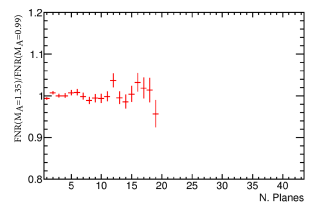
Figure 5: (color online) The FNR systematic distortion due to different modeling of the neutrino interaction. An extreme value has been chosen for the axial-mass, $M_{A}=1.35$ GeV, compared to the standard one, $M_{A}=0.99$ GeV. The distortion is shown as function of the crossed iron planes of the detector (see Section 4); it corresponds to the systematic error due to the convolution of the neutrino interaction, the fluxes and the detectors’ acceptance.

Table 2: Systematic uncertainties on the FNR estimator as function of the crossed iron planes due to the convolution of the neutrino interaction, the fluxes and the detectors’ acceptance, as shown in Fig. 5, up to a muon momentum of about 1 GeV. Uncertainties average at 0% with a spread $<$ 1% due to the discreetness of the variable used.

nb. pl.	(%)	nb. pl.	(%)	nb. pl.	(%)
0	-0.63	4	0.7	8	-0.5
1	0.7	5	0.9	9	-0.6
2	0	6	-0.1	10	-0.1
3	0.1	7	-1.1	11	3.7

3.3 Monte Carlo beam simulation

In order to evaluate how the hadro–production uncertainty affects the knowledge of the FNR in our experiment a new beam–line simulation was developed. The angular and momentum distribution of pions exiting the Be target were simulated using either FLUKA (2011.2b) fluka or GEANT4 (v4.9.4 p02, QGSP 3.4 physics list). Furthermore the Sanford–Wang parametrization for $\pi^{+}$ determined from a fit of the HARP and E910 data–set in G4BNBflux , was used:

$$\frac{d^{2}\sigma}{dpd\Omega}=c_{1}p^{c_{2}}\left(1-\frac{p}{p_{b}-1}\right)e^{-\frac{p^{c_{3}}}{p_{b}^{c_{4}}}-c_{5}\theta(p-c_{6}p_{b}\cos^{c_{7}}\theta)}$$ (1)

with $p_{b}$ being the proton–beam momentum and $c_{i}$ ($i=1\ldots$ 7) free parameters. The additional subdominant contributions arising from $\pi^{-}$ and $K$ decays have been neglected when considering positive polarity beam configurations.

For the propagation and decays of secondary mesons a simulation using GEANT4 libraries was developed. A simplified version of the beam–line geometry was adopted. Despite the approximations a fair agreement with the official simulation of the MiniBooNE Collaboration G4BNBflux was obtained. This tool is sufficient for the purpose of the site optimization that is described in the following. In order to fully take into account finite–distance effects, fluxes and spectra were derived after extrapolating neutrinos down to the detector volumes without using weighing techniques. A total number of $7\times 10^{8}$ protons on target (p.o.t.), $2.1\times 10^{8}$ p.o.t. and $1\times 10^{9}$ pions were simulated with FLUKA, GEANT4 and Sanford–Wang parametrization, respectively.

In Fig. 6 the transverse distributions of neutrinos at a distance of 110 m from the target is shown. The root–mean–square (r.m.s.) of the distribution is about 5 m. The projected coordinate is shown in the bottom plot of Fig. 6 with a Gaussian fit superimposed for comparison. The plot indicates that a near detector placed on ground–surface ($Y=7$ m) would severely limit the statistics (furthermore the angular acceptance of the far and near detectors would be too different).

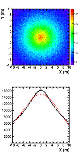
Figure 6: (color online) The neutrino beam profile at 110 m from the target. In the bottom plot the projection on the horizontal axis, $X$, fitted to a Gaussian curve for comparison.

3.4 Choice of experimental sites

Once the geometry and the mass of the detectors have been fixed additional issues affect the choice of the location of the experimental sites, near and far ones. The ultimate figure of merit is the power of exclusion (or discovery) for effects induced by sterile neutrinos in a range of parameters as wide as possible in a given running time.

As soon as the detectors are further away from the target they “see” more similar spectra since the production region better approximates a point–like source. This helps in reducing the systematic uncertainty. On the other hand the larger is the distance the smaller is the size of the collected event sample. Moreover the lever–arm for oscillation studies is reduced. The reliability of the simulation of the neutrino spectra at the near and far sites remains an essential condition. This point is further addressed in Section 3.4.2.

On a practical basis the increasing of the depth of the detector sites impacts considerably on the civil engineering costs. Furthermore existing or proposed experimental facilities (SciBooNE/LAr1–ND, T150–Icarus, MiniBooNE, MicroBooNE, LAr1, Icarus) already partially occupy possible sites along the beam line SBN .

3.4.1 Dependence of $\nu_{\mu}^{CC}$ rates and energy spectra on the detector position

The $\nu_{\mu}^{CC}$ interaction rates and their mean energy depend on the distance from the proton target, as shown in Fig. 7, top and bottom, respectively.

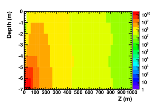
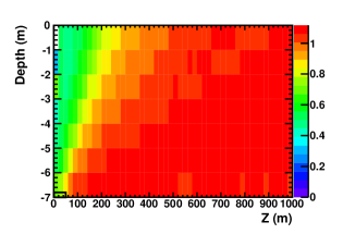
Figure 7: (color online) Top: $\nu_{\mu}^{CC}$ rate (a.u.) vs distance from the target, $Z$, and the depth from the ground surface. Bottom: mean energy (in GeV) of $\nu_{\mu}^{CC}$ interactions vs $Z$ (m) and depth. The origin of the reference system is the proton–target upstream position. The hollow box close to the origin indicates the longitudinal extension of the decay pipe.

The horizontal axis corresponds to the distance ($Z$) from the target, the vertical axis to the depth from the ground surface. At a distance of about 700 m the rates and the mean energies are barely affected when moving from on–axis to off–axis positions. That consideration supports the possibility of placing the far detector on surface, thus reducing the experiment cost.

3.4.2 Systematics in the near–to–far ratio for a set of detector configurations

Six configurations were selected considering different distances (110, 460 and 710 m), either on–axis or off–axis, and different fiducial sizes of the detectors. The configurations’ parameters are given in Tab. 3 and illustrated schematically in Fig. 8.

Table 3: Near–Far detectors’ configurations. $L_{N(F)}$ is the distance of the near (far) detector from the target. $y_{N(F)}$ is the vertical coordinate of the center of the near (far) detector with respect to the beam axis, which lies at about $-$7 m from the ground surface. $s_{N(F)}$ is the transverse size of the near (far) detector.

config.	$L_{N}$ (m)	$L_{F}$ (m)	$y_{N}$ (m)	$y_{F}$ (m)	$s_{N}$ (m)	$s_{F}$ (m)
1	110	710	0	0	4	8
2	110	710	0	0	1.25	8
3	110	710	1.4	11	4	8
4	110	710	1.4	11	1.25	8
5	460	710	7	11	4	8
6	460	710	6.5	10	4	6

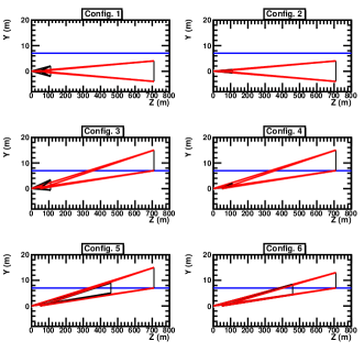
Figure 8: (color online) Configurations of far and near detectors in the $Y$–$Z$ plane (see also Tab. 3). The blue horizontal line marks the ground level, the vertical black lines mark the detectors and the red lines show the angle subtended by the detectors at the beginning and the end of the decay pipe.

• Configuration 1 corresponds to two detectors on–axis at 110 (near) and 710 m (far) with squared active areas of $4\times 4$ m² (near) and $8\times 8~{}\rm{m}^{2}$ (far). By selecting the subsample of neutrinos crossing both the near and far detectors the region defined in the transverse plane has roughly a squared shape with a significant “blurring” since the neutrino source is not point–like.

• Configuration 2 make use of a reduced near detector area, limited to $1.25\times 1.25$ m², in order to increase the fraction of neutrinos seen both at the near and far sites.

• Configurations 3 and 4 replicate the same patterns as 1 and 2, respectively, with the far detector on surface and the size of the near detector defined by the off–axis angle (instead of being both on–axis).

• Configurations 5 and 6 are similar to 3 and 4, respectively, but with the near site at a larger distance (460 m).

Using FLUKA, GEANT4 or the Sanford–Wang parametrization for the simulation of $p$–Be interactions, the FNR was computed for each configuration (Fig. 9).

In configuration 1 (on–axis detectors and a large near–detector size) the FNR increases with energy, as expected from the discussion in Section 3.2, largely departing from a flat curve. By reducing the transverse size of the near detector (configuration 2) the FNR flattens out. This same behavior is confirmed using off–axis detectors (configurations 3 and 4). Even flatter FNRs are obtained in configurations with a near detector at larger baselines (5 and 6). The different behaviors are more evident in Fig. 10, where the FNRs based on the Sanford–Wang parametrization and normalized to each other are compared.

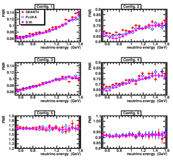
Figure 9: (color online) Far–to–Near ratios for each considered configuration. Comparison of results from the different hadro–productions simulations by FLUKA, GEANT4 and the Sanford–Wang parametrization are shown. The error bars indicate only the uncertainty introduced by the limited Monte Carlo samples of FLUKA and GEANT4. The barely visible error bars on the Sanford–Wang points are due to the very large number of simulated pions.

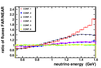
Figure 10: (color online) Far–to–Near ratios for the six considered configurations using the Sanford–Wang parametrization.

In order to estimate the impact on the FNR of the hadro–production uncertainties two studies were made.

First, the difference in the hadronic models implemented in the FLUKA and GEANT4 generators were looked at. For each configuration the FNR predictions from these two Monte Carlo simulations are drawn in Fig. 11 as their ratio. The (yellow) bands correspond to a fixed 3% error on the FNR ratios between FLUKA and GEANT4. The two simulations agree at 1 to 3% level when an overlapping region between the far and near detectors occurs (configurations 2, 4 and 6).

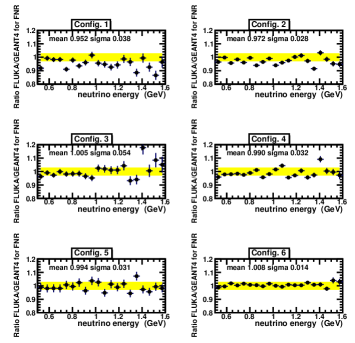
Figure 11: Ratio of the two FNRs as predicted by the FLUKA and GEANT4 simulations for hadro–production. The bands correspond to a 3% relative error on the different predictions by FLUKA and GEANT4.

Another approach was adopted to investigate the FNR systematic–error due to hadro–production based on the existing measurements and the corresponding covariance–error matrix of Booster Be–target replica G4BNBflux . The coefficients $c_{i}$ of the Sanford–Wang parametrization of pion production data from HARP and E910 in Eq. 1 were sampled within their correlation errors. The sampling of these correlated parameters was performed via the Cholesky decomposition of the covariance matrix reported in Tab. 5 of G4BNBflux . For each sampling of the $c_{i}$ coefficients, neutrinos were weighted with a factor

$$w(p_{\pi},\theta_{\pi})=\frac{\frac{d\sigma}{dp_{\pi}d\theta_{\pi}}(c_{i})}{\frac{d\sigma}{dp_{\pi}d\theta_{\pi}}(c^{0}_{i})}$$ (2)

depending on the momentum ($p_{\pi}$) and angle ($\theta_{\pi}$) of their parent pion. $c^{0}_{i}$ are the best–fit values to the HARP–E910 data–set. The FNR for different $c_{i}$ varied within their covariance error–matrices are shown in Fig. 12 for the six considered configurations.

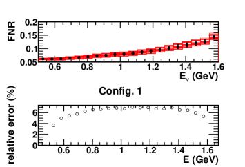
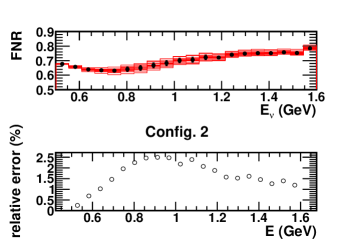
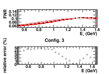
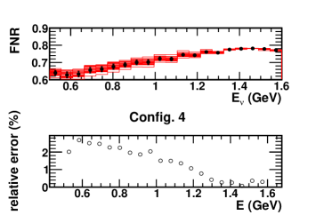
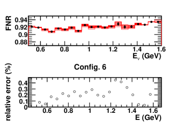
Figure 12: The FNR results for the six configurations are shown as function of the neutrino energy. The effect of data–driven hadro–production uncertainties on the FNR computed using the Sanford–Wang parametrization for the six configurations is depicted. Histogram lines show typical individual–samplings of the $c_{i}$ parameters of Eq. 1. Plain bullets correspond to the average value in each bin while the error bars represent the r.m.s. of the samplings. For each configuration, bottom plots (hollow bullets) show the ratios of the r.m.s. over the central values, providing an estimate of the fractional systematic error.

For each configuration, in the top plots (plain bullets) the average value is shown with its error bar representing the r.m.s. of the samplings. Bottom plots (hollow bullets) show the ratio of the r.m.s. over the central value providing an estimate of the fractional systematic error. Uncertainties are rather large (5–7%) when considering the full area of the near detector at 110 m; they decrease significantly when restricting to the central region (configurations 2, 4 and 6). In particular, in configuration 4, that is a realistic one from practical considerations, the uncertainty ranges from 2% at low neutrino energy and decreases below 0.5% –1.5% at neutrino energies above 1 GeV. The uncertainty is generally below 0.5% for a near site at 460 m.

3.5 Conclusions for Section 3

Full simulations of the Booster beam were made anew, based on FLUKA and GEANT4 Monte Carlo simulations. Indications of the systematic error on the far–to–near ratio were obtained, showing characteristic behaviours. Moreover, using the constraints from HARP–E910 data the uncertainties on the FNR, associated to hadro–production, were carefully estimated.

Six configurations of the detector locations and sizes were considered. For a far detector on ground–surface and a near detector at the same off-axis angle the systematic error stays at 1–2% when the far and near transverse surfaces are matched in acceptance (configuration 4). Provided the high available statistics and the large lever–arm for oscillation studies, the layout with baselines of 110 m and 710 m is considered in the following as the best choice.

4 Detector Design Studies

The location of the Near and Far sites is a fundamental issue in a search for sterile neutrino at SBL. Moreover the two detector systems at the two sites have to be as similar as possible. The NESSiE far and near spectrometer system were designed to match with a timely schedule and also exploit the experience acquired in the construction, assembling and maintenance of the OPERA spectrometers bopera that own an active transverse area of $8.75\times 8.00$ m² .

The OPERA two large dipole iron magnets will be dismantled in 2015–2016 and possibly be re-used for the $\nu_{\mu}$ disappearance study discussed in this paper. They are made of two vertical arms connected by a top and a bottom return yoke. Each arm is composed of 12 planes of 5 cm thick iron slabs, interleaved by 11 planes of Resistive Plate Chambers (RPC) that provide the inner tracker. The magnetic field has opposite directions in the two arms and is uniform in the tracking region, with an intensity of 1.53 T.

Muons stopping in the spectrometers can be identified by their range. Their fraction can be maximized by increasing the depth of the magnets. This can be achieved by longitudinally coupling the two OPERA spectrometers, both at the far and the near sites, minimizing therefore the detector re–design. Their modularity allows to cut every single piece at 4/7 of its height, using the bottom part for the far site and the top part for near site. In this way any inaccuracy in geometry (the single 5 cm thick iron slab owns a precision of few mm) or any variation of the material properties with respect to the nominal ones (they are at the level of few percent) will be the same in the two detection sites. The near NESSiE spectrometer will thus be a clone of the far one, with identical thickness along the beam but a reduced transverse size.

With the proposed setup a very large fraction of muons from CC neutrino interactions is stopped in the spectrometer. For this class of events the momentum is obtained by muon range. For higher energies the muon momentum is determined from the muon track sagitta measured in the bending plane. The charge of the muon can be determined when its track crosses few RPC planes ($\geq$ 3). The distributions of hit RPC planes are shown in Fig. 13 for charged and neutral current events.

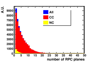
Figure 13: (color online) Number of crossed RPC planes for charged and neutral current events (5 cm slab geometry).

In the positive–mode running of the Booster beam the antineutrino contamination is rather low (see Fig. 14). In this case the use of the charge identification is limited and it can contribute only to keep the related systematic error under control and well below 1% since the mis–identification of the charge (mis—ID) of the Spectrometers is about 2.5% in the relevant momentum range (see the bottom plot of Fig. 24). The situation is quite different for the negative–mode running where the neutrino contamination is rather high (see Section 6).

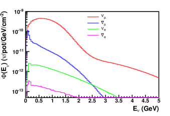
Figure 14: (color online) The fluxes of the Booster neutrino beam (from G4BNBflux ).

In the following the performances (efficiency and purity) of the spectrometer with 5 cm thick iron–slabs are evaluated in terms of Neutral Current (NC) contamination and momentum resolution, and compared to a geometry with 2.5 cm thick iron slabs.

With 5 cm slabs the fraction $\varepsilon$ of neutrino interactions in iron inducing at least one RPC hit ($\varepsilon\equiv{(\geq 1RPC)}/{all}$) is 68%. The efficiency for CC and NC events is $\varepsilon_{CC}=86\%$ and $\varepsilon_{NC}=20\%$, respectively. That corresponds to a fraction of NC interactions over the total number of interaction ${NC}/{all}=8.1\%$. With a minimal cut of 2 crossed RPC planes, the NC contamination is reduced to 4.2%; by requiring 3 RPC planes the NC contamination drops to 3.0%.

Using 2.5 cm thick slabs, the fraction of neutrino events with at least one RPC hit increases for both NC and CC events. The CC efficiency and the NC contamination are both larger with respect to the 5 cm geometry. In Fig. 15 $\varepsilon_{CC}$ and the purity, $CC/all=1-NC/all$, are shown as a function of the minimum number of crossed RPC planes, for either slab thickness.

At the same level of purity the efficiencies in the two geometries are comparable. No advantage in statistics is obtained with thinner slabs if the same NC contamination suppression is required. In conclusion the already available 5 cm thick iron slabs can be adopted. It is worthwhile to note that purities and efficiencies have been extensively checked not to be spoiled by second-order systematic effects due to the convolution of the fluxes and the neutrino cross-section with the detector acceptances at the two sites. That keeps the systematic error due to the neutrino detection below 1% while the most relevant contribution to systematics remains the uncertainty on the fluxes.

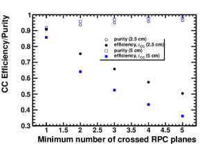
Figure 15: CC efficiency ($\varepsilon_{CC}$) and purity as a function of the minimum number of hit RPC planes for the two spectrometer geometries, 5 cm thick iron slabs (squares) and 2.5 cm thick slabs (circles).

4.1 Track and momentum reconstruction

The RPC digital read–out is provided on both vertical ($Y$) and horizontal ($X$) coordinates using 2.6 cm pitch strips. Track reconstruction is made first in the two RPC projections (the $XZ$ bending plane, and the $YZ$ plane). Then, the two 2–D tracks are merged to reconstruct a 3–D event.

For muons stopping inside the spectrometer the momentum is obtained from the track range using the continuous–slowing–down approximation pdg . The range distribution is shown in Fig. 16. Similar conclusions can be drawn as for the number of crossed RPC planes (in Fig. 13), namely the CC efficiency and the reduction of the NC related background.

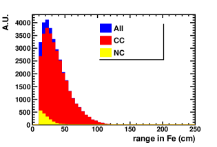
Figure 16: (color online) Muon range of reconstructed events, for CC plus NC (blue), CC (red) and NC (yellow) events.

For any muon track a parabolic fit is performed in the bending plane to evaluate the track sagitta thus determining particle charge and momentum.

In Fig. 17 (CC events) the reconstructed variables, namely the number of fired RPC planes and the range in iron, are plotted versus the muon momentum. A correlation is visible for both variables. The very strong muon momentum–range linear correlation allows to reach a sensitivity of few percent in the momentum estimation.

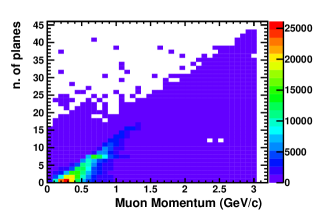
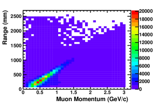
Figure 17: (color online) Number of crossed RPC planes (top) and range (bottom) versus muon momentum (CC events).

4.2 Conclusions for Section 4

In the previous Section 3 it was shown that by adopting a realistic layout configuration, and by a proper choice of the fiducial volume at the near site, a reduction of the uncertainty on the Far/Near ratio to less than 2% level is possible, by plugging the data–driven knowledge on hadro–production (HARP and E910 G4BNBflux ). This is by far the dominant component. Possible other effects due to the running conditions of the detectors once installed can be kept under control ($<1\%$). It must be noted that the efficiency and acceptance of the spectrometers can be checked routinely with good accuracy using the large amount of available cosmic rays. Furthermore the detector in itself is very well mastered and understood due to its simplicity and to the extensive experience in running it underground on the CNGS beam. Furthermore, each original (from OPERA) iron slab will be used partly at the near and partly at the far site, providing the same geometrical and material composition. That choice would provide a very constrained system at the two sites, with not only identical targets, but also similar geometrical frames and acceptances. The relative large statistical sample that could be obtained within configuration 4 would allow a careful control of the related systematic effects, by operating at different energy ranges, too. Finally, all the effects due to detector acceptance and event–reconstruction have been evaluated to be within 1%.

5 Physics Analyses and Performances

The disappearance probability of muon–neutrinos, $P(\nu_{\mu}\to{\rm not}\,\nu_{\mu})$, in presence of an additional sterile–state can be expressed in terms of the extended PMNS pmns mixing matrix ($U_{\alpha i}$ with $\alpha=e,\mu,\tau,s$, and $i=1,\ldots,4$). In this model, called “3+1”, the neutrino mass eigenstates $\nu_{1},\ldots,\nu_{4}$ are labeled such that the first three states are mostly made of active flavour states and contribute to the “standard” three flavour oscillations with the squared mass differences $\Delta m_{21}^{2}\sim 7.5\times 10^{-5}~{}{\rm eV^{2}}$ and $|\Delta m_{31}^{2}|\sim 2.4\times 10^{-3}~{}{\rm eV^{2}}$, where $\Delta m_{ij}^{2}=m^{2}_{i}-m^{2}_{j}$. The fourth mass eigenstate, which is mostly sterile, is assumed to be much heavier than the others, $0.1~{}{\rm eV^{2}}\lesssim\Delta m_{41}^{2}\lesssim 10~{}{\rm eV^{2}}.$ The opposite case in hierarchy, i.e. negative values of $\Delta m_{41}^{2}$, produces a similar phenomenology from the oscillation point of view but is disfavored by cosmological results on the sum of neutrino masses cosmo-data .

In a Short-Baseline experiment the oscillation effects due to $\Delta m^{2}_{21}$ and $\Delta m^{2}_{31}$ can be neglected since $L/E\sim 1$ km/GeV. Therefore the oscillation probability depends only on $\Delta m^{2}_{41}$ and $U_{\alpha 4}$ with $\alpha=e,\mu,\tau$. In particular the survival probability of muon neutrinos is given by the effective two–flavour oscillation formula:

$$P(\nu_{\mu}\to\nu_{\mu})_{SBL}^{3+1}=1-\left[4|U_{\mu 4}|^{2}(1-|U_{\mu 4}|^{2})\right]\sin^{2}\frac{\Delta m^{2}_{41}L}{4E},$$ (3)

where $4|U_{\mu 4}|^{2}(1-|U_{\mu 4}|^{2})$ is the amplitude and, since the baseline $L$ is fixed by the experiment location, the oscillation phase is driven by the neutrino energy E.

In contrast, appearance channels (i.e. $\nu_{\mu}\to\nu_{e}$) are driven by terms that mix up the couplings between the initial and final flavour–states and the sterile state, yielding a more complex picture:

$$P(\nu_{\mu}\to\nu_{e})_{SBL}^{3+1}=4|U_{\mu 4}|^{2}|U_{e4}|^{2}\sin^{2}\frac{\Delta m^{2}_{41}L}{4E}$$ (4)

Similar formulas hold also assuming more sterile neutrinos ($3+n$ models).

Since $|U_{\alpha 4}|$ is expected to be small, the appearance channel is suppressed by two more powers in $|U_{\alpha 4}|$ with respect to the disappearance one. Furthermore, since $\nu_{e}$ or $\nu_{\mu}$ appearance requires $|U_{e4}|>0$ and $|U_{\mu 4}|>0$, it should be naturally accompanied by non–zero $\nu_{e}$ and $\nu_{\mu}$ disappearances. In this sense the disappearance searches are essential for providing severe constraints on the theoretical models (a more extensive discussion on this issue can be found e.g. in Section 2 of winter ).

It should also be noticed that a good control of the $\nu_{e}$ contamination is important when using the $\nu_{\mu}\to\nu_{e}$ for sterile neutrino searches at SBL. In fact the observed number of $\nu_{e}$ neutrinos would depend on the $\nu_{\mu}\rightarrow\nu_{e}$ appearance and also on the $\nu_{e}\rightarrow\nu_{s}$ disappearance. On the other hand, the amount of $\nu_{\mu}$ neutrinos would be affected by the $\nu_{\mu}\rightarrow\nu_{s}$ and $\nu_{e}\rightarrow\nu_{\mu}$ transitions. However the latter term ($\nu_{\mu}$ appearance) would be much smaller than in the $\nu_{e}$ case since the $\nu_{e}$ contamination in $\nu_{\mu}$ beams is usually at the percent level. In conclusion in the $\nu_{\mu}$ disappearance channel the oscillation probabilities in either the near or far detector are not affected by any interplay of different flavours. Since both near and far detectors measure the same single disappearance transition, the probability amplitude is the same at both sites.

Another important aspect of the analysis is related to the procedure of either rejecting or evaluating the presence of a sterile component. The basic hypothesis of no-sterile oscillation ($H_{0}$) has been assumed against the presence of something else ($H_{1}$). For $H_{0}$ the analysis is simplified since the systematic errors on the FNR estimator are definitively under control when no-sterile component is included, as illustrated in the previous sections. In particular the cross-section uncertainties, the hadro-production modeling, the beam–flux variations and their convolutions with the detectors’ acceptance have been checked: the systematic error on FNR is $1-2\%$. Evaluation of p-values for $H_{0}$ allows to set the possible presence of a sterile component. However, in order to estimate the power of an experiment exclusion plots should be also evaluated. The distortion of FNR due to a sterile neutrino component with respect to the null hypothesis has been looked through, taking care of the correlations due to the systematic errors. In the following both procedures are depicted.

The experiment sensitivity to the $\nu_{\mu}$ disappearance was evaluated by considering several estimators, related either to i) the muon produced in $\nu_{\mu}^{CC}$ or to ii) the reconstructed neutrino energy. The muon momentum can be very effective when $H_{0}$ hypothesis is checked to establish the probability of the non-sterile component, i.e. the observation of something else. In such a case the simulation is limited to the standard processes and the FNR approach in the NESSiE environment is fully efficient. Instead, to evaluate exclusion plots one needs to extract the oscillation parameters via Monte Carlo by looking at the FNR distortion in specific regions of the phase space. A new procedure based on the reconstructed muon momentum was also implemented to exclude regions defined by new “effective” variables. Using reconstructed measured quantities allows to keep systematic errors under control.

In the second case (ii) the neutrino energy was reconstructed from

$$E_{\nu}=\frac{E_{\mu}-m^{2}_{\mu}/(2M)}{1-(E_{\mu}-p_{\mu}\cos\theta)/M},$$ (5)

valid in the Charge Current Quasi Elastic (CCQE) approximation, $M$ being the nucleon mass, $E_{\mu}$ and $p_{\mu}$ the muon energy and momentum, respectively.

We developed complex analyses to determine the sensitivity region that can be explored with an exposure of $6.6\times 10^{20}$ p.o.t., corresponding to 3 years of data collection on the FNAL–Booster beam. Our guidelines were the maximal extension at small values of the mixing angle parameter and the control of the systematic effects.

The sensitivity of the experiment was evaluated performing three analyses that implement different techniques and approximations:

• method I: a Feldman&Cousins technique (see Section V of Fel-Cou ) with ad hoc systematic errors added to the muon momentum distribution;

• method II: a Pearson’s $\chi^{2}$ test pdg with a full correlation matrix based on full Monte Carlo simulation and reconstruction;

• method III: a new approach based on the profile likelihoods, often referred to as modified frequentist method or CL_s read-2002 , similar to that used in the Higgs boson discovery atlas-cms .

Throughout the analyses the detector configuration defined in Table 4 was considered.

Table 4: Fiducial mass and baselines in configuration 4 for near and far detectors, used for the sensitivity analyses.

	Fiducial Mass (ton)	Baseline (m)
Near	297	110
Far	693	710

The distributions of events, either in $E_{\nu}$ or $p_{\mu}$, normalized to the expected luminosity in 3 years of data taking ($6.6\times 10^{20}$ p.o.t.) with the FNAL–Booster beam running in positive focusing mode, are reported in Fig. 18.

The study of the $\overline{\nu}_{\mu}$ disappearance is reported in Section 6 with results obtained from method III.

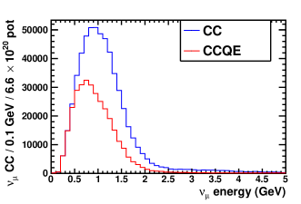
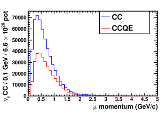
Figure 18: (color online) The total number of expected $\nu_{\mu}$ CC interactions seen by the Far detector at 710 m, as a function of $E_{\nu}$ (top) and $p_{\mu}$ (bottom), for the expected luminosity in 3 years of data taking ($6.6\times 10^{20}$ p.o.t.) with the FNAL–Booster beam in positive–mode running. The sub–sample corresponding to the CCQE component is also shown.

5.1 Sensitivity Analyses

In the three analyses the two–flavour neutrino mixing in the approximation of one mass dominance was considered. The oscillation probability is given by:

$$P({\nu_{\mu}\to\nu_{\mu}})=1-\sin^{2}(2\theta_{new})\sin^{2}\left(\frac{1.27\Delta m^{2}_{new}L[{\rm km}]}{E[{\rm GeV}]}\right),$$ (6)

where $\Delta m^{2}_{new}$ is the mass splitting between a new heavy–neutrino mass–state and the heaviest among the three SM neutrinos, and $\theta_{new}$ is the corresponding effective mixing angle.

In the selected procedures (Feldman&Cousins approach, $\chi^{2}$ test with Near–Far correlation matrix and CL_s profile likelihoods) the evaluation of the sensitivity region to sterile neutrinos was computed at 95% C.L. Some recent use of more stringent Confidence Limits (even to 10 $\sigma$’s nustorm ) was judged un–necessary, provided the correct and conservative estimation of the systematic errors. Besides, we note that the measurement of muon tracks is a quite old and proven technique with respect to the more difficult detection and measurement of electron–neutrino interactions in Liquid–Argon systems.

5.1.1 Method I (Feldman&Cousins technique)

In method I the far–to–near ratio was written as $R_{i}=F_{i}/(kN_{i})$, where $F_{i}$ and $N_{i}$ are the number of events in the $i$–th bin of the muon–momentum distribution in the far and near detectors, respectively, and $k$ is a bin–independent constant factor used to normalize each other the near and far distributions. For each value of the oscillation parameters, $\sin^{2}2\theta_{new}$ and $\Delta m^{2}_{new}$, the $\chi^{2}$ is computed as

$$\chi^{2}=\sum_{i=1}^{N}\left(\frac{1-R_{i}/R_{0,i}}{\sigma_{R_{0,i}}}\right)^{2},$$ (7)

where $R_{0,i}$ is the far–to–near ratio in absence of oscillation and $\sigma_{R_{0,i}}$ is the quadratic sum of the statistical error and a fixed, bin–to–bin uncorrelated, systematic error. In the Feldman&Cousins approach a $\Delta\chi^{2}_{cut}(\sin^{2}2\theta_{new},$ $\Delta m^{2}_{new})=\chi^{2}(\sin^{2}2\theta_{new},\Delta m^{2}_{new})-\chi^{2}_{min}$ cut is applied. For every ($\sin^{2}2\theta_{new}$, $\Delta m^{2}_{new}$) oscillated spectra were generated and fitted to obtain the $\chi^{2}_{min}$. The distribution of $\Delta\chi^{2}(\sin^{2}2\theta_{new},\Delta m^{2}_{new})$ is cut at 95% to define the $(\sin^{2}2\theta_{new},\Delta m^{2}_{new})$ exclusion region. The critical value on $\Delta\chi^{2}_{cut}$ can be determined by either sampling the $\Delta\chi^{2}$ distribution as in Feldman&Cousins or by applying the standard $\chi^{2}_{cut}$ fixed–value for the 95% C.L. and two degrees–of–freedom. It was verified that in both cases the obtained results are very similar in the whole ($\sin^{2}2\theta_{new}$, $\Delta m^{2}_{new}$) space.

Results are shown in Fig. 19 for a set of ten simulated null experiments. In the top plot a systematic error $\epsilon_{sys}=0$ was used. In the bottom plot a bin–to–bin uncorrelated systematic–error $\epsilon_{sys}=0.01$ was assumed (see Section 12.1 of nessie-fnal for more details).

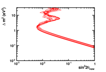
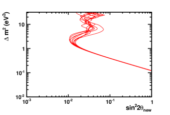
Figure 19: Top: sensitivity curves at 95% C.L. with ten simulated toy experiments and no systematic uncertainties. In the fit procedure $p_{\mu}$ was used as observable with a cut of 500 MeV/c. 10⁴ sampling points, uniformly distributed in log scale, were generated. The expected integrated luminosity for 3 years of data taking ($6.6\times 10^{20}$ p.o.t.) with the FNAL–Booster beam in positive–mode running was assumed. Bottom: as above but using a bin–to–bin uncorrelated systematic–error $\epsilon_{sys}=0.01$.

5.1.2 Method II ($\chi^{2}$ test with Near–Far correlation matrix)

In method II the sensitivity to the $\nu_{\mu}$ disappearance was evaluated using two different observables, the muon range and the number of crossed RPC planes. The correlations between the data collected in the far and near detectors are taken into account through the covariant matrix of the observables. The $\chi^{2}$ is given by

$$\chi^{2}=\sum_{i=1}^{N}\sum_{j=0}^{N}\left(kN_{i}-F_{i}\right)\left(M^{-1}\right)_{ij}\left(kN_{j}-F_{j}\right),$$ (8)

where $M$ is the covariance matrix covM of the uncertainties (statistical and bin–to–bin systematic correlations covM2 ).

The $\nu_{\mu}$ disappearance can be observed either by a deficit of events (normalization) or, also, by a distortion of the observable spectrum (shape), which are affected by systematic uncertainties expressed by the normalization error–matrix and the shape error–matrix, respectively. The shape error–matrix represents a migration of events across the bins. In this case the uncertainties are associated with changes not affecting the total number of events. Consequently, a depletion of events in some region of the spectrum should be compensated by an enhancement in others. Details of the model used for the shape error–matrix can be found in nessie-fnal .

The distributions of the muon range and of the number of crossed planes were computed using GLoBES GLoBES with the smearing matrices obtained by the full Monte Carlo simulation described in Section 4.

By applying the frequentist method the $\chi^{2}$ statistic distribution was looked at in order to compute the sensitivity to oscillation parameters. Different cuts on the range and on the number of crossed planes were studied. Furthermore sensitivity plots were computed by introducing bin–to–bin correlated systematic uncertainties by considering either 1% correlated error in the normalization or alternatively 1% correlated error in the spectrum shape.

As a representative result the sensitivity computed using the range as observable and taking the 1% correlated error in the shape, is plotted in Fig. 20. Instead the normalization correlated–error would slightly reduce the sensitivity region around $\Delta m^{2}_{new}=1$ eV². Moreover, the sensitivity region obtained by using the sum of CC and NC events is almost the same as that obtained with CC events only (see Section 12.2 in nessie-fnal ). That proves that the result is not affected by the NC background events.

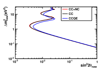
Figure 20: (color online) 95% C.L. sensitivity obtained using the muon range for all the interaction processes (Quasi Elastic, Resonant, Deep Inelastic Scatering): CC (black), CC+NC (red) and for CCQE events only (blue). 1% bin–to–bin correlated error in the shape is considered. The expected integrated luminosity for 3 years of data taking ($6.6\times 10^{20}$ p.o.t.) with the FNAL–Booster beam in positive–mode running was assumed.

5.1.3 Method III (CL_s profile likelihoods)

In the profile CL_s method we introduce a new test–statistics that depends on a signal–strength variable. By looking at Eq. 6 the factor $\sin^{2}2\theta_{new}$ acts as an amplification quantity for a fixed $\Delta m^{2}_{new}$. Therefore a signal–strength $\mu$ can be identified with $\sin^{2}2\theta_{new}$ to construct the estimator function:

$$f=\frac{1-\mu\cdot\sin^{2}(1.27\ \Delta m^{2}_{new}\ L_{Far}/E_{\nu})}{1-\mu\cdot\sin^{2}(1.27\ \Delta m^{2}_{new}\ L_{Near}/E_{\nu})}.$$ (9)

In a simplified way, for each $\Delta m^{2}_{new}$, a sensitivity limit on $\mu$ can be obtained from the p–value of the distribution of the estimator $f$ in Eq. 9, in the assumption of background–only hypothesis.

That procedure does not correspond to computing the exclusion region of a signal, even if it provides confidence for it. The exclusion plot should be obtained by fully developing the CL_s procedure as described in Section 12.3 of nessie-fnal . However, since we are here mainly interested in exploiting the sensitivity of the experiment, the procedure provides already insights into that. Its result comes fully compatible with the previous two analyses, which follow the usual neutrino analyses found in the literature.

Moreover, following the same attitude, an even more aggressive procedure can be applied. Since the deconvolution from $p_{\mu}$ to $E_{\nu}$ introduces a reduction of the information, we investigated whether the more direct and measurable parameter, $p_{\mu}$, can be a valuable one. In such a case Eq. 9 becomes:

$$f=\frac{1-\mu\cdot\sin^{2}(1.27\ \Delta m^{2}_{new}\ L_{Far}/p_{\mu})}{1-\mu\cdot\sin^{2}(1.27\ \Delta m^{2}_{new}\ L_{Near}/p_{\mu})}$$ (10)

The corresponding sensitivity plot is shown in Fig. 21. It provides an “effective” sensitivity limit in the “effective” variables $\Delta m^{2}$ and the reconstructed muon momentum, $p_{\mu,rec}$. By applying the Monte Carlo deconvolution from $p_{\mu,rec}$ to $E_{\nu}$ we checked that the “effective” $\Delta m^{2}$ is simply scaled–off towards lower values, not affecting the mixing angle limit. The merits of the $p_{\mu,rec}$ are multiple: it is not affected as $E_{\nu}$ by the propagation error due to the deconvolution process, the systematics errors due to the reconstruction of the events (efficiency, acceptance, background) are directly included since it corresponds to a measured quantity, the estimator is powerful in identifying a possible new signal/anomaly.

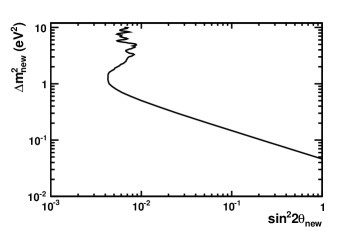
Figure 21: The sensitivity at 95% of C.L. obtained by computing the modified raster–scan method, in a CL_s framework, and by using the reconstructed muon momentum as estimator (equation (10)). The expected integrated luminosity for 3 years of data taking ($6.6\times 10^{20}$ p.o.t.) with the FNAL–Booster beam in positive–mode running was assumed. A conservative cut of $p_{\mu,rec}\geq\ 500$ MeV/c was applied.

5.2 Conclusions for Section 5

The sensitivity curves obtained with different analyses prove the possibility to explore a very large region in the mass–scale and mixing–angle plane, larger than other current proposals. Using a configuration with two (massive) detectors, one at 110 m on–axis, and one at 710 m off-axis (configuration 4, see Table 4), the achievable sensitivity curves are drawn in Fig. 22 for several C.L., compared to existing limits mini-sci-mu ; recent-MINOS and the predicted sensitivities of the SBN project SBN . A systematic error of 1% has been assumed and a conservative cut $p_{\mu,rec}\geq\ 500$ MeV/c was applied. A sensitivity to mixing angles below $10^{-2}$ in $\sin^{2}2\theta_{new}$ can be obtained in a large region of $\Delta m^{2}$ around $1\ {\rm eV}^{2}$ scale.

It is noted that by applying more elaborated reconstruction algorithms than those used in the present analysis the 500 MeV/c cut in $p_{\mu,rec}$ could be lowered to $200-300$ MeV/c. The exclusion region could then be significantly extended to $\Delta m^{2}<1$ eV², even if systematic errors should generally be larger and therefore detailed studies would be required to really access that limit.

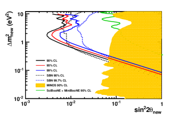
Figure 22: The sensitivity curves obtained using the modified raster–scan method (equation (9)), in a CL_s framework, for 90%, 95% and 99.7% C.L., for an expected integrated luminosity of 3 years of data taking ($6.6\times 10^{20}$ p.o.t.) with the FNAL–Booster beam in positive–mode running. An uncorrelated 1% systematic error and a conservative cut of $p_{\mu,rec}\geq\ 500$ MeV/c were used. The filled area corresponds to the MINOS recent-MINOS result and the green curve to the MiniBooNE/SciBooNE mini-sci-mu limit (at 90% C.L.). The two dashed lines corresponds to the sensitivity predicted by the new SBN proposal  SBN , at 90% and 99.7% C.L.

We demonstrated that a sophisticated statistical tool (method III) can be applied to get hints of new neutrino states at lower mass–scale than that achievable with the usual ones (methods I and II), by making use of a different estimator (the reconstructed muon momentum), less dependent of the Monte Carlo simulation. Thus we conclude that, on top of the exclusion limits, a robust confidence is accomplished on the identification of a possible new signal.

6 Sensitivity for the antineutrino disappearance

In negative–focusing mode the Booster beam contains a large neutrino component. In terms of flux the contamination amounts to 15% at 1 GeV, 30% at 1.5 GeV and surpasses the antineutrino flux above 2 GeV (see Fig. 23). In this energy region the measurement of the charge on event–by–event basis is an efficient tool. Although a comprehensive study of the spectrometers’ ultimate performance goes beyond the scope of this paper, we estimated the improvement on the final sensitivity by using their charge ID capability. We applied Method III of Section 5.1.3, under some additional assumptions on the neutrino–antineutrino components. The contamination of the neutrino events resulting from the charge mis–ID probability ($\eta$) was included in an uncorrelated way to the near and far data samples, with/without the assumption that only antineutrinos oscillate. The assumption that the oscillation phenomenon acts differently for neutrinos and antineutrinos puts limits on their possible correlated oscillation probabilities. Though the resulting sensitivity curves correspond to the worst case scenario, they provide a decoupled insight into the possible measurement of the antineutrino disappearance at 1 eV mass–scale and small mixing angle, for the first time.

For the antineutrino disappearance search two main results exist, an old one by the CCFR experiment ccfr-anti and more recent ones from the MiniBooNE mini-mu and MiniBooNE/SciBooNE mini-sci-antimu . The MiniBooNE results come with a 20%–25% contamination of the intrinsic neutrino flux and were obtained assuming that only antineutrinos oscillate while neutrinos do not.

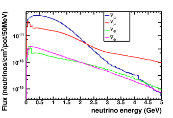
Figure 23: (color online) The flux components of the Booster antineutrino beam (from G4BNBflux ).

A total integrated luminosity corresponding to 3 years of running at the Booster in negative–focusing mode was considered. The number of events that could be collected at the far detector is displayed in Fig. 24. The neutrino sub–component is highly enhanced because of its larger cross-section with respect to the antineutrino one.

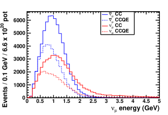
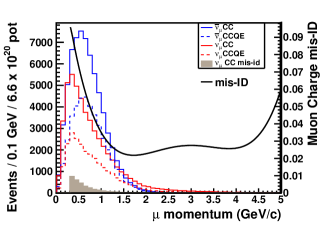
Figure 24: (color online) The total number of foreseen $\overline{\nu}_{\mu}$ CC interactions seen by the Far detector at 710 m, as function of the $E_{\nu}$ (top) and the $p_{\mu}$ (bottom), for the expected luminosity in 3 years of data taking ($6.6\times 10^{20}$ p.o.t.) with the FNAL–Booster beam in negative–mode running. Separate antineutrino and neutrino data are shown, with also the sub–samples corresponding to the CCQE component (dashed histograms). In the bottom plot the mis–ID of the muon charge as provided by the spectrometers, is overlaid (black curve and left scale) bopera . The grey zone in the same plot corresponds to the expected CC neutrino contamination once measured the muon track (integrated 3200 over 58600 CC events in the 0.3 – 5 GeV interval).

To evaluate our sensitivity to the signal–strength estimator (Section 5.1.3) a set of four samples has been considered, under different assumptions:

1)

the pure anti-neutrino sample (perfect rejection of neutrino contamination);

2)

the anti-neutrino sample with the neutrino contamination as determined by the spectrometers charge mis-ID. The same oscillation law is assumed for neutrinos and anti-neutrinos;

3)

as above, but assuming no oscillation for the neutrino contamination;

4)

the anti-neutrinos sample with full neutrino contamination (no charge ID), assuming no oscillation for the neutrino contamination.

Fig. 25 shows the corresponding sensitivity curves, that have less and less power going from assumption (1) to (4), as expected. The most sensitive curve (case 1 and red line) corresponds to the pure sample of antineutrinos. The black line for case (2) is obtained by including the muon charge mis-ID in the collected event sample and increasing correspondingly the statistical errors associated to the neutrino and anti-neutrino components. The curve for case 3 (blue line) is obtained by assuming that the neutrino component, identified by the muon charge, do not oscillate, then decreasing the total sample while contributing to the statistical error. The purple line for (4) indicates the sensitivity in case the neutrino component is not identified and assumed not oscillating.

The key feature of the charge identification is apparent since the quite small contamination coming from the mis–ID produces small corrections. In contrast lacking of charge measurement oblige to assume an oscillation pattern for the contamination component and reduces drastically the amount of the equivalent statistical sample and the sensitivity region (case 4).

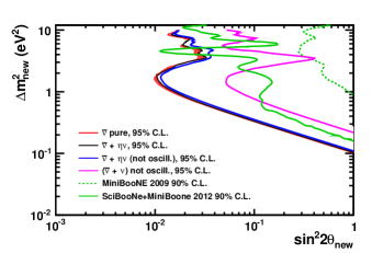
Figure 25: (color online) The four sensitivity curves (see text for explanation) obtained using the modified raster–scan method (equation (9)), in a CL_s framework, for 95% C.L., for an expected integrated luminosity of 3 years of data taking ($6.6\times 10^{20}$ p.o.t.) with the FNAL–Booster beam running in negative–focusing mode. $\eta$ stays for the charge mis–ID probability. An uncorrelated 1% systematic error and a conservative cut of $p_{\mu,rec}\geq\ 500$ MeV/c were used. Previous results are also shown. The dashed green curve corresponds to the 90% C.L MiniBooNE mini-mu limit while the plain green curve corresponds to its improved analysis and data collection with also the SciBooNE data mini-sci-antimu .

7 Conclusions

Existing anomalies in the neutrino sector may hint to the existence of one or more additional sterile neutrino states. A detailed study of the physics case was performed to set up a Short–Baseline experiment at the FNAL–Booster neutrino beam exploiting the study of the muon–neutrino charged–current interactions. An independent measurement on $\nu_{\mu}$, complementary to the already proposed experiments on $\nu_{e}$, is mandatory to either prove or reject the existence of sterile neutrinos, even in case of null result for $\nu_{e}$. Moreover, very massive detectors are mandatory to collect a large number of events and therefore improve the disentangling of systematic effects.

The best option in terms of physics reach and funding constraints is provided by two spectrometers based on dipoles iron magnets, at the Near and Far sites, located at 110 (on–axis) and 710 m (on surface, off–axis) from the FNAL–Booster neutrino source, respectively, possibly placed behind the proposed LAr detectors.

A full re-use of the OPERA spectrometers, when dismantled, would be feasible. Each site at FNAL can host a part of the two coupled OPERA magnets, based on well know technology, allowing to realize “clone” detectors at the Near and Far sites. The spectrometers would be equipped with RPC detectors, already available, which have demonstrated their robustness and effectiveness.

With that configuration one would succeed in keeping the systematic error at the level of $1-2$% for the measurements of the $\nu_{\mu}$ interactions, i.e. the measurement of the muon–momentum at the percent level and the identification of its charge on event–by–event basis, extended to well below 1 GeV.

The achieved sensitivity on the mixing angle between the standard neutrinos and a new state is well below 0.01 for the $\nu_{\mu}$ mode. The measurement of the muon charge on event–by–event basis has been demonstrated to be very efficient for the estimation of possible disappearance antineutrino phenomena, for the first time at the level of few percents for the mixing angle and a mass scale around 1 eV.

References

- (1) We quote here the most recent papers on the measurement of : F. An et al. (DAYA–BAY Collaboration), Phys. Rev. Lett. 112, 061801 (2014), arXiv:1310.6732; S. H. Seo et al. (RENO Collaboration), Proceedings Neutrino2014, Boston, USA (2014), arXiv:1410.7987; Y. Abe et al. (DOUBLE–CHOOZ Collaboration), J. High Energy Phys. 10, 086 (2014), arXiv:1406.7763; K. Abe et al. (T2K Collaboration), Phys. Rev. Lett. 112, 181801 (2014), arXiv:1311.4750.
- (2) B. Pontecorvo, Zh. Eksp. Teor. Fiz. 53, 1717 (1967) [Sov. Phys. JETP 26, 984 (1968)].
- (3) K. Abazajian, M. Acero, S. Agarwalla, A. Aguilar-Arevalo, C. Albright et al., arXiv:1204.5379.
- (4) J. Kopp, P. A. N. Machado, M. Maltoni, and T. Schwetz, J. High Energy Phys. 05, 050 (2013), arXiv:1303.3011; T. Schwetz, Nucl. Phys. B 235–236, 2292235 (2013); C. Giunti, M. Laveder, Y. F. Li, Q. Y. Liu, and H. W. Long, Phys. Rev. D 86, 113014 (2012).
- (5) F. Dydak et al. (CDHS Collaboration), Phys. Lett. B 134, 281 (1984).
- (6) A. A. Aguilar–Arevalo et al. (MiniBooNE Collaboration), Phys. Rev. Lett. 103, 061802 (2009), arXiv:0903.2465.
- (7) K. B. M. Mahn et al. (MiniBooNE and SciBooNE Collaborations), Phys. Rev. D 85, 032007 (2012), arXiv:1106.5685. G. Cheng et al., Phys. Rev. D 86, 052009 (2012), arXiv:1208.0322.
- (8) A. Sousa (MINOS Collaboration), proceedings to Neutrino2014, Boston, USA (2014), arXiv:1502.07715; A. Timmons (MINOS Collaboration), proceedings to NuPhys2014, London, UK (2014), arXiv:1504.04046; P. Adamson et al. (MINOS Collaboration), Phys. Rev. Lett. bf 117, 151803 (2016), arXiv:1607.01176v4.
- (9) R. Wendell (Super–K Collaboration) contributions to Neutrino2014, Boston, USA (2014); K. Abe et al. (Super–K Collaboration), Phys. Rev. D 91, 052019 (2015), arXiv:1410.2008.
- (10) I. E. Stockdale et al, (CCFR Collaboration), Phys. Rev. Lett. 52, 1384 (1984).
- (11) P. Adamson et al., (MINOS and DAYA-BAY Collaborations), Phys. Rev. Lett. 117, 151801 (2016), arXiv:1607.01177.
- (12) M. G. Aartsen et al., (IceCube Collaboration) Phys. Rev. Lett. 117, 071801 (2016), arXiv:1605.01990.
- (13) M. Nessi et al., https://edms.cern.ch/nav/P:CERN-0000077383:V0/P:CERN-0000096728:V0/TAB3.
- (14) P5 reports in http://science.energy.gov/hep/hepap/reports/.
- (15) M. Antonello et al. (ICARUS Collaboration), arXiv:1312.7252.
- (16) C. Adams et al. (LAr1–ND Collaboration), FNAL–P–1053 (2013) and arXiv:1309.7987v3.
- (17) MicroBooNE Experiment, http://www-microboone.fnal.gov/.
- (18) M. Antonello et al. (ICARUS, LAr1-ND and MicroBooNE Collaborations), arXiv:1503.01520.
- (19) P. Bernardini et al. (NESSiE Collaboration), SPSC–P–343 (2011), arXiv:1111.2242.
- (20) M. Antonello et al. (ICARUS and NESSiE Collaborations), SPSC–P–347 (2012), arXiv:1203.3432.
- (21) L. Stanco et al., Ad. High Energy Phys., 948626 (2013), arXiv:1306.3455v2.
- (22) A. Anokhina et al. (NESSiE Collaborations), FNAL–P–1057 (2014), arXiv:1404.2521.
- (23) A. A. Aguilar–Arevalo et al. (MiniBooNE Collaboration), Phys. Rev. D 79, 072002 (2009), arXiv:hep-ex/0806.1449v1.
- (24) S. E. Kopp., arXiv:hep-ex/0712.1280.
- (25) C.Andreopoulos et al., The GENIE Neutrino Monte Carlo Generator, Nucl. Instrum. Meth. A614, 87 (2010).
- (26) A. Ferrari, P. R. Sala, A. Fassò, J. Ranft, Reports No. CERN-2005-10, 2005, No. INFN/TC-05/11, and No. SLAC-R-773, www.slac.stanford.edu/cgi-wrap/getdoc/slac-r-773.pdf; G. Battistoni, F. Cerutti, A. Fassò, A. Ferrari, S. Muraro, J.Ranft, S. Roesler, and P. R. Sala, AIP Conf. Proc. 896, 31 (2007); G. Battistoni, A. Margiotta, S. Muraro, and M. Sioli, Nucl. Instrum. Meth. Phys. Res., Sect. A 626-627, S191 (2011) [see, also, www.fluka.org].
- (27) A. A. Aguilar-Arevalo et al. (SciBooNE Collaboration), arXiv:hep-ex/0601022.
- (28) R. Acquafredda et al. (OPERA collaboration), JNST 4, 4018 (2009).
- (29) C. Amsler et al. (Particle Data Group), Phys. Lett. B 667, 1 (2008).
- (30) B. Pontecorvo, Sov. Phys. JETP 26, 984 (1968); Z. Maki, M. Nakagawa, and S. Sakata, Prog. Theor. Phys. 28, 870 (1962).
- (31) P.A.R. Ade et al. (Planck Collaboration), submitted to A&A (2015), arXiv:1502.01589v2.
- (32) W. Winter, Phys. Rev. D 85, 113005 (2012), arXiv:1204.2671.
- (33) G. J. Feldman and R. D. Cousins, Phys. Rev. D 57, 3873 (1998), http://arxiv.org/abs/physics/9711021v2.
- (34) A. L. Read, Jou. .Phys., G 28, 2693 (2002).
- (35) ATLAS and CMS Collaborations, LHC Higgs Combination Group, ATL–PHYS–PUB–2011–1, CMS NOTE–2011/005,
- (36) D. Adey et al. (nuSTORM Collaboration), Phys. Rev. D 89, 071301(R).
- (37) K. Mahn, Ph.D. thesis, Columbia University (2009).
- (38) M. G. Aartsen et al. (IceCube Collaboration), arXiv:1409.4535.
- (39) P. Huber, M. Lindner, and W. Winter, Comput. Phys. Commun. 167, 195 (2005), http://www.mpi-hd.mpg.de/personalhomes/globes/index.html.
- (40) I. E. Stockdale et al, (CCFR Collaboration), Z.Phys. C27 53 (1985).
- (41) G. Cheng et al., Phys. Rev. D 86, 052009 (2012), arXiv:1208.0322.