The cylindrical $K$-function and Poisson line cluster point processes

Abstract

The analysis of point patterns with linear structures is of interest in many applications. To detect anisotropy in such cases, in particular in case of a columnar structure, we introduce a functional summary statistic, the cylindrical $K$-function, which is a directional $K$-function whose structuring element is a cylinder. Further we introduce a class of anisotropic Cox point processes, called Poisson line cluster point processes. The points of such a process are random displacements of Poisson point processes defined on the lines of a Poisson line process. Parameter estimation based on moment methods or Bayesian inference for this model is discussed when the underlying Poisson line process is latent. To illustrate the methodologies, we analyze two- and three-dimensional point pattern data sets. The three-dimensional data set is of particular interest as it relates to the minicolumn hypothesis in neuroscience, claiming that pyramidal and other brain cells have a columnar arrangement perpendicular to the surface of the brain.

1 Introduction

Frequently in the spatial point process literature, isotropy, i.e., distributional invariance under rotations about a fixed location in space, is assumed, though it is often unrealistic. Anisotropy of spatial point processes has usually been studied by summarizing the information of observed pairs of points, including the use of directional $K$-functions or related densities (Ohser & Stoyan, 1981; Stoyan & Beneš, 1991; Stoyan, 1991; Stoyan & Stoyan, 1995; Guan et al., 2006; Illian et al., 2008; Redenbach et al., 2009), spectral and wavelet methods (Mugglestone & Renshaw, 1996; Rosenberg, 2004; Nicolis, Mateu & D’Ercole, 2010), and geometric anisotropic pair correlation functions (Møller & Toftaker, 2014). The applications considered in these references except Redenbach et al. (2009) and Illian et al. (2008) are for two-dimensional but not three-dimensional point patterns.

There are point patterns where points lie approximately along straight lines, cf. the examples of applications and references in Møller & Waagepetersen (2016), called point patterns with linear structures. This paper focuses on detecting and modelling such point patterns observed within a bounded subset of $\mathbb{R}^{d}$, $d\geq 2$, where the cases $d=2$ and $d=3$ are of main interest. In particular we study columnar structures.

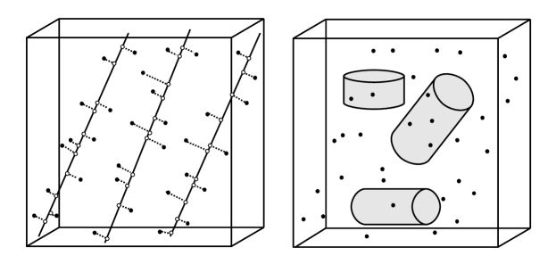
Section 2 introduces the cylindrical $K$-function, a directional $K$-function whose structuring element is a cylinder which is suitable for detecting anisotropy caused by columnar or other linear structures in spatial point patterns. This is an adapted version of the space-time $K$-function (Diggle et al., 1995; Gabriel & Diggle, 2009). Section 3 concerns a new class of point processes, Poisson line cluster point processes, whose points cluster around a Poisson line process. The left panel in Figure 1 illustrates how such a process is constructed: lines are generated from an anisotropic Poisson line process, independent stationary Poisson point processes are generated on the lines, and their points are randomly displaced, resulting in the Poisson line cluster point process. We consider the Poisson lines and the points on the lines as latent, so the clusters of the Poisson line cluster point process are also hidden. Section 3 also discusses a moment based approach and a simulation-based Bayesian approach for inference, where in the latter case we estimate both the parameters of the model and the missing lines.

Figure 1: Poisson line cluster process: Left panel: A simulated realization of a Poisson line cluster point process within a three-dimensional box. The realizations of the Poisson line process (solid lines) and the Poisson point processes on the lines (circles) are also shown. The dotted lines indicate how the points on the lines have been displaced to new positions (filled circles) and they specify the clusters. Right panel: The same simulated realization of a Poisson line cluster point process and different choices of cylinders centered at different points of the process.

Sections 2-3 apply our methodology to the data sets in Figure 2. The left panel shows a two-dimensional point pattern data set recorded by Mugglestone & Renshaw (1996), namely the locations of 110 chapels in the Welsh Valleys, United Kingdom, where the clear linear orientation is caused by four more or less parallel valleys. For a three-dimensional point pattern data set it is often difficult to detect anisotropy by eye, but the cylindrical $K$-function will be useful, as illustrated later in connection to the right panel, which shows the locations of 623 pyramidal cells from the Brodmann area 4 of the grey matter of the human brain collected by the neuroscientists at the Center for Stochastic Geometry and Bioimaging, Denmark. According to the minicolumn hypothesis (Mountcastle, 1957), brain cells, mainly pyramidal cells, should have a columnar arrangement perpendicular to the pial surface of the brain, i.e., a columnar arrangement parallel to the $x^{(3)}$-axis indicated in Figure 2, and this should be highly pronounced in Brodmann area 4. However, this hypothesis has been much debated, see Rafati et al. (2016) and the references therein.

Figure 2: Data sets: Left panel: Locations of 110 chapels in Wales, United Kingdom, observed in a square window (normalized to a unit square). Right panel: Nucleolus of 623 pyramidal cells in an observation window of size $508\times 138\times 320\,\mu{m}^{3}$.

We use the chapel data set mainly for illustrative purposes and for comparison with previous work. Investigations of the minicolumn hypothesis have so far only been done in two dimensions except for the three-dimensional analysis in Rafati et al. (2016). The present paper details the methodology and provides a more thorough analysis of the pyramidal cell data set, shedding further light on the validity of the minicolumn hypothesis.

Throughout Sections 2–3 we assume stationarity. Section 4 discusses the choice of a cylinder as the structuring element of the $K$-function and extensions of this function and the Poisson line cluster point process in a non-stationary setting.

2 The cylindrical $K$-function

2.1 Setting

Throughout this paper we make the following assumptions and use the following notation.

Unless otherwise stated, we consider a stationary point process $X$ defined on $\mathbb{R}^{d}$, with finite and positive intensity $\rho$, and where we view $X$ as a locally finite random subset of $\mathbb{R}^{d}$. Here stationarity means that the distribution of $X$ is invariant under translations in $\mathbb{R}^{d}$, and $\rho|B|$ is the mean number of points from $X$ falling in any Borel set $B\subseteq\mathbb{R}^{d}$ of volume $|B|$. We assume that $X$ has a pair correlation function $g(x)$ defined for all $x\in\mathbb{R}^{d}$. Intuitively, if $x_{1},x_{2}\in\mathbb{R}^{d}$ are distinct locations and $B_{1},B_{2}$ are infinitesimally small sets of volumes $\mathrm{d}x_{1},\,\mathrm{d}x_{2}$ and containing $x_{1},x_{2}$, respectively, then $\rho^{2}g(x_{1}-x_{2})\,\mathrm{d}x_{1}\,\mathrm{d}x_{2}$ is the probability for $X$ having a point in each of $B_{1}$ and $B_{2}$. For further details on spatial point processes, see Møller & Waagepetersen (2004) and the references therein.

We view any vector $x=(x^{(1)},\ldots,x^{(d)})\in\mathbb{R}^{d}$ as a column vector, and $\|x\|=\{(x^{(1)})^{2}+\ldots+(x^{(d)})^{2}\}^{1/2}$ as its length. For ease of presentation, we assume that no pair of distinct points $\{x_{1},x_{2}\}\subset X$ is such that $u=(x_{1}-x_{2})/\|x_{1}-x_{2}\|$ is perpendicular to the $x^{(d)}$-axis. This will happen with probability one for the models considered later in this paper.

Let $\mathbb{S}^{d-1}=\{u=(u^{(1)},\ldots,u^{(d)})\in\mathbb{R}^{d}:\,\|u\|=1\}$ be the unit sphere in $\mathbb{R}^{d}$ and $e_{d}=(0,\ldots,0,1)$ its top point. Denote $o=(0,\ldots,0)$ the origin of $\mathbb{R}^{d}$. Consider the $d$-dimensional cylinder with midpoint $o$, radius $r>0$, height $2t>0$, and direction $e_{d}$:

$$C(r,t)=\left\{x=(x^{(1)},\ldots,x^{(d)})\in\mathbb{R}^{d}:\,(x^{(1)})^{2}+\cdots+(x^{(d-1)})^{2}\leq r^{2},\,|x^{(d)}|\leq t\right\}.$$

For $u\in\mathbb{S}^{d-1}$, denoting $\mathcal{O}_{u}$ an arbitrary $d\times d$ rotation matrix such that $u=\mathcal{O}_{u}e_{d}$, then

$$C_{u}(r,t)=\mathcal{O}_{u}C(r,t)$$

is the $d$-dimensional cylinder with midpoint $o$, radius $r$, height $2t$, and direction $u$.

2.2 The cylindrical $K$-function

Recall that the second order reduced moment measure $\mathcal{K}$ with structuring element $B\subset\mathbb{R}^{d}$, a bounded Borel set, is given by

$$\mathcal{K}(B)=\int_{B}g(x)\,\mathrm{d}x$$

(Møller & Waagepetersen, 2004, Section 4.1.2). Ripley’s $K$-function (Ripley, 1976, 1977) is obtained when $B$ is a ball and it is not informative about any kind of anisotropy in a spatial point pattern.

To detect preferred directions of linear structures in a spatial point pattern, in particular a columnar structure, we propose a cylinder as the structuring element and define the cylindrical $K$-function in the direction $u$ by

$$K_{u}(r,t)=\int_{C_{u}(r,t)}g(x)\,\mathrm{d}x,\quad u\in\mathbb{S}^{d-1},\quad r>0,\ t>0.$$ (1)

Intuitively, $\rho K_{u}(r,t)$ is the mean number of further points in $X$ within the cylinder with midpoint at the typical point of $X$, radius $r$, and height $2t$ in the direction $u$. For example, a stationary Poisson process is isotropic, has $g=1$, and

$$K_{u}(r,t)=2\omega_{d-1}r^{d-1}t,$$

where $\omega_{d-1}=\pi^{(d-1)/2}/\Gamma\{(d+1)/2\}$ is the volume of the $({d-1})$-dimensional unit ball. For $d=3$, $K_{(0,0,1)}$ is similar to the space-time $K$-function in Diggle et al. (1995) and Gabriel & Diggle (2009), when considering the $x^{(3)}$-axis as time and the $(x^{(1)},x^{(2)})$-plane as space.

If $W\subset\mathbb{R}^{d}$ is an arbitrary Borel set with $0<|W|<\infty$, then by standard methods (Møller & Waagepetersen, 2004, Section 4.1.2)

$$K_{u}(r,t)=\frac{1}{\rho^{2}|W|}\,E\left[\sum_{x_{1},x_{2}\in X:\,x_{1}\not=x_{2}}\mathbb{1}\{x_{1}\in W,x_{2}-x_{1}\in C_{u}(r,t)\}\right],\quad r>0,\ t>0,$$ (2)

where $\mathbb{1}$ denotes the indicator function, and by stationarity the right-hand side does not depend on the choice of $W$. This provides a more general definition of $K_{u}$, since (2) does not require the existence of the pair correlation function. Equation (2) becomes useful when deriving non-parametric estimates in Section 2.3.

2.3 Non-parametric estimation

Given a bounded observation window $W\subset\mathbb{R}^{d}$ and an observed point pattern $\{x_{1},\ldots,x_{n}\}\subset W$ with $n\geq 2$ points, we consider non-parametric estimates of the form

$$\widehat{K}_{u}(r,t)=\frac{1}{\widehat{\rho^{2}}}\sum_{i\not=j}w_{u}(x_{i},x_{j})\mathbb{1}\{x_{j}-x_{i}\in C_{u}(r,t)\}.$$ (3)

Here $\widehat{\rho^{2}}$ is a non-parametric estimate of $\rho^{2}$ and $w_{u}$ is an edge correction factor. If $X$ is isotropic, $K_{u}(r,t)$ does not depend on $u$ and this should affect the choice of $\widehat{K}_{u}(r,t)$. On the other hand, as illustrated in the right panel of Figure 1 and in Section 2.4, to detect a preferred direction of linearity in a spatial point pattern, we suggest using an elongated cylinder with $t>r$ and considering different directions $u$. Then we expect a largest value of $\widehat{K}_{u}(r,t)$ to indicate the preferred direction, but a careful choice of $r$ and $t$ may be crucial, cf. Section 4. Furthermore, since $K_{u}=K_{-u}$, we need only to consider the case where $u=(u^{(1)},\ldots,u^{(d)})$ is on the upper unit-sphere, i.e., $u^{(d)}\geq 0$.

Specifically, we use $\widehat{\rho^{2}}=n(n-1)/|W|^{2}$, see e.g. Illian et al. (2008), and the translation correction factor (Ohser & Stoyan, 1981)

$$w_{u}(x_{1},x_{2})=1/|W\cap W_{x_{2}-x_{1}}|$$ (4)

where $W_{x}$ denotes translation of the set $W$ by a vector $x\in\mathbb{R}^{d}$. Then, by Lemma 4.2 in Møller & Waagepetersen (2004), if $\widehat{\rho^{2}}$ is replaced by $\rho^{2}$ in (3), we have an unbiased estimate of $K_{u}$. As in Figures 1–2, if $W$ is rectangular with sides parallel to the axes and of lengths $a_{1},\ldots,a_{d}>0$,

$$|W\cap W_{x_{2}-x_{1}}|=\prod_{i=1}^{d}\{a_{i}-|x_{2}^{(i)}-x_{1}^{(i)}|\},\quad x_{1},x_{2}\in W,$$

where $x_{j}^{(i)}$ denotes the $i$’th coordinate of $x_{j}$ $(j=1,2)$.

For $d=3$, $W=[0,a_{1}]\times[0,a_{2}]\times[0,a_{3}]$, and $u=(0,0,1)$, another choice is a combined correction factor

$$w_{(0,0,1)}(x_{1},x_{2})=\frac{1+\mathbb{1}\left(2x_{1}^{(3)}-x_{2}^{(3)}\not\in[0,a_{3}]\right)}{a_{3}\left(a_{1}-\left|x_{2}^{(1)}-x_{1}^{(1)}\right|\right)\left(a_{2}-\left|x_{2}^{(2)}-x_{1}^{(2)}\right|\right)}$$

where the numerator is a temporal correction factor and the denominator is the reciprocal of a spatial correction factor; similarly we construct combined correction factors when $u=(1,0,0)$ or $u=(0,1,0)$. Instead of this spatial correction factor, which is of a form similar to (4), Diggle et al. (1995) used an isotropic correction factor, but this is only appropriate if $X$ is isotropic in the $(x_{1},x_{2})$-plane. The temporal correction factor is the same as that used in Diggle et al. (1995).

We prefer the translation correction factor (4), since this does not restrict the shape of $W$ and the choice of $u$. In a simulation study with $d=3$, $W=[0,1]^{3}$, and $X$ a Poisson line cluster point process as defined in Section 3, we obtained similar results when using the translation and the combined correction factors.

2.4 Examples

Non-parametric estimates of the cylindrical $K$-function for the two-dimensional chapel data set and the three-dimensional pyramidal cell data set are shown in Figures 3 and 4, respectively. Below we comment on these plots. Further examples are given in Rafati et al. (2016).

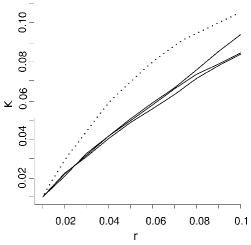
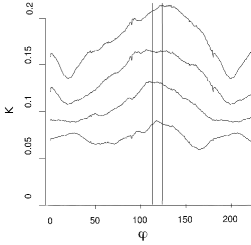
To detect the main direction in the chapel point pattern, the left panel in Figure 3 shows, for four different combinations of $r$ and $t$, i.e., $(0.1,0.2)$, $(0.1,0.3)$, $(0.2,0.3)$ and $(0.2,0.4)$, plots of $\widehat{K}_{u}(r,t)$ versus $\varphi$, where $u=(\cos(\varphi),\sin(\varphi))$. These four curves are approximately parallel, and a similar behaviour for other choices of $r=0.05,0.1,0.15,0.2$ and $t=0.15,0.2,0.25,0.3,0.35,0.4$ with $t>2r$ was observed. In a previous analysis, Møller & Toftaker (2014) estimated the orientation of the chapel point pattern to be between $113^{\circ}$ and $124^{\circ}$. This interval, which is specified by the vertical lines in the left panel of Figure 3, is in close agreement with the maximum of the $\widehat{K}_{u}(r,t)$-curves. The middle panel in Figure 3 shows plots of $\widehat{K}_{u}(r,t)$ versus $r$ when $t=0.3$. For the dotted curve in the middle panel, $\varphi=117^{\circ}$ is the average of the four maximum points of $\varphi$ corresponding to the four curves in the left panel, while for the three other curves in the middle panel, values of $\varphi$ not included in the interval $[113^{\circ},124^{\circ}]$ have been chosen. The clear difference between the dotted curve and the other curves indicates a preferred direction in the point pattern which is about $117^{\circ}$. This is also confirmed by the right panel in Figure 3, which shows a non-parametric estimate of the point pair orientation distribution function given by equation (14.53) in Stoyan & Stoyan (1995) and implemented in spatstat (Baddeley & Turner, 2005). This is a kernel estimate which considers the direction for each pair of observed points that lie more than $r_{1}=0.05$ and less than $r_{2}=0.15$ units apart. For other values of $r_{2}\leq 0.27$ we reached similar conclusions, but for higher values of $r_{2}$ the pair orientation distribution function did not show a clear preferred direction in the data.

Figure 3: Chapel data set: The left panel shows the non-parametric estimate $\widehat{K}_{(\cos\varphi,\sin\varphi)}(r,t)$ versus $\varphi$ for four different combinations of $r$ and $t$ with the curves from the top to the bottom corresponding to $(r,t)=(0.2,0.4),(0.2,0.3),(0.1,0.3),(0.1,0.2)$ and the two vertical lines corresponding to $113^{\circ}$ and $124^{\circ}$. The middle panel shows $\widehat{K}_{(\cos\varphi,\sin\varphi)}(r,t)$ versus $r$ for different values of $\varphi$ and with $t=0.3$ with the solid curves from the top to the bottom corresponding to $20^{\circ},45^{\circ},170^{\circ}$, and the dotted curve corresponding to $\varphi=117^{\circ}$. The right panel shows a non-parametric estimate of the point pair orientation distribution function with $r_{1}=0.05$ and $r_{2}=0.15$. For more details, see Section 2.4.

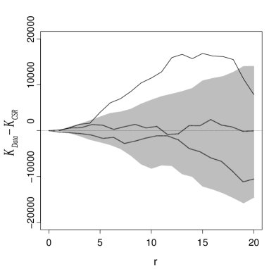
By the minicolumn hypothesis, the pyramidal cell data set has a columnar arrangement in the direction of the $x^{(3)}$-axis indicated in Figure 2 (Rafati et al., 2016). Figure 4 shows that the cylindrical $K$-function is able to detect this kind of anisotropy: The three curves are $\widehat{K}_{u}(r,80)-160\pi r^{2}$ for $0<r\leq 20$ and $u$ parallel to one of the three main axes, where $160\pi r^{2}$ is the value of $K_{u}(r,80)$ under complete spatial randomness, i.e. a stationary Poisson point process model; we only make this comparison in order to see any deviations from complete spatial randomness. The solid curve corresponding to $u=(0,0,1)$, i.e., when the direction of the cylinder is along the $x^{(3)}$-axis, is clearly different from the two other cases where $u=(1,0,0)$ or $u=(0,1,0)$. The grey region is a so-called 95% simultaneous rank envelope (Myllymäki et al., 2016) obtained from $999$ simulated realizations under complete spatial randomness; Myllymäki et al. (2016) recommended 2499 simulations, however, for the cylindrical $K$-function considered in Figure 4, 999 simulations seemed sufficient since results were produced that were similar to those using 2499 simulations. Roughly speaking, under complete spatial randomness, each of the estimated cylindrical $K$-functions is expected to be within the grey region with estimated probability 95%. While the curves for $u=(1,0,0)$ and $u=(0,1,0)$ are completely within the grey region, the curve for $u=(0,0,1)$ is clearly outside for a large range of $r$-values. In fact, for the null hypothesis of complete spatial randomness, considering the rank envelope test (Myllymäki et al., 2016) based on $\widehat{K}_{u}(r,80)$ when $0<r\leq 20$ and $u=(0,0,1)$, the $p$-value is estimated to be between $0.1\%$ and $0.18\%$, showing a clear deviation from the null hypothesis of complete spatial randomness.

Figure 4: Pyramidal cell data set: Non-parametric estimates $\widehat{K}_{u}(r,80)-160\pi r^{2}$ versus $r$ when $t=80$ and the cylinder is along the $x^{(1)}$-axis (dotted line), the $x^{(2)}$-axis (dotted line), or the $x^{(3)}$-axis (solid line). The grey region specifies a $95\%$ simultaneous rank envelope computed from 999 simulations under complete spatial randomness. For more details, see Section 2.4.

These examples illustrate that the cylindrical $K$-function is a useful functional summary statistic for detecting preferred directions and columnar structures in a spatial point pattern. Particularly, for the pyramidal cell data set and in accordance to the minicolumn hypothesis, there is a pronounced columnar arrangement in the direction of the $x^{(3)}$-axis.

3 The Poisson line cluster point process

3.1 Definition of Poisson line cluster point processes

Motivated by the analysis in Section 2.4, in particular that of the pyramidal cell data set, we now introduce a model for a point process $X$ with columnar structure. It is a hierarchical construction, using various latent processes specified briefly in (A1)–(C1) and later in more detail in (A2)–(C2), while $X$ is given in (D1) and (D2) below; the left panel of Figure 1 is helpful in this connection: It consists of generating:

(A1)

a Poisson line process $L=\{l_{1},l_{2},\ldots\}$ of lines $l_{i}$, i.e., infinite, directed, and straight lines; only parts of these lines are shown in Figure 1;

(B1)

on each line $l_{i}$, a Poisson process $Q_{i}$ illustrated by unfilled points in Figure 1;

(C1)

a new point process $X_{i}$ obtained by random displacements in $\mathbb{R}^{d}$ of the points in $Q_{i}$ illustrated by filled points in Figure 1;

(D1)

finally, $X$ as the superposition of all the $X_{i}$.

Then we call $X$ a Poisson line cluster point process, since its points cluster around the Poisson lines, and we call each $X_{i}$ a cluster.

In connection to the more detailed conditions (A2)–(D2) we need the following notation. Let $\cdot$ denote the usual inner product on $\mathbb{R}^{d}$. For $u\in\mathbb{S}^{d-1}$, let $u^{\bot}=\{x\in\mathbb{R}^{d}:\,x\cdot u=0\}$ be the hyperplane perpendicular to $u$ and containing $o$, $\lambda_{u^{\bot}}$ the $(d-1)$-dimensional Lebesgue measure on ${u^{\bot}}$, and $p_{u^{\bot}}(x)=x-(x\cdot u)u$ the orthogonal projection of $x\in\mathbb{R}^{d}$ onto ${u^{\bot}}$. Let $H={e_{d}^{\bot}}$ and $\lambda=\lambda_{e_{d}^{\bot}}$, i.e., $H$ is the hyperplane perpendicular to the $x^{(d)}$-axis. Further, let $k$ be a density function with respect to Lebesgue measure on $\mathbb{R}^{d-1}$. As in Section 2.1, suppose we have specified for each $u\in\mathbb{S}^{d-1}$ a $d\times d$ rotation matrix $\mathcal{O}_{u}$ such that $u=\mathcal{O}_{u}e_{d}$. We then define a density with respect to $\lambda_{u^{\bot}}$ by

$$k_{u^{\bot}}\{\mathcal{O}_{u}(x^{(1)},\ldots,x^{(d-1)},0)\}=k(x^{(1)},\ldots,x^{(d-1)}),\quad(x^{(1)},\ldots,x^{(d-1)})\in\mathbb{R}^{d-1}.$$

In other words, when considering coordinates with respect to the $d-1$ first columns in $\mathcal{O}_{u}$, the distribution under $k_{u^{\bot}}$ is the same as under $k$. Furthermore, for the line process $L$ we use the so-called phase representation (Chiu et al., 2013) and assume that with probability one, $L$ has no line contained in $H$. Thereby a line $l=l(y,u)$ in $L$ corresponds to its direction $u\in\mathbb{S}^{d-1}$ and its intersection point $y$ in $H$. Thus $L=\{l_{1},l_{2},\ldots\}$ can be identified by a point process $\Phi=\{(y_{1},u_{1}),(y_{2},u_{2}),\ldots\}\subset H\times\mathbb{S}^{d-1}$ such that $l_{i}=l(y_{i},u_{i})$ $(i=1,2,\ldots)$ and $\Phi\subset H\times(\mathbb{S}^{d-1}\setminus H)$ almost surely.

In addition to (A1)–(D1) we assume that:

(A2)

$\Phi$ is a Poisson process with intensity measure $\beta\lambda(\mathrm{d}y)M(\mathrm{d}u)$, where $\beta>0$ is a parameter and $M$ is a probability measure on $\mathbb{S}^{d-1}$ describing the direction of a typical line, where $M(\mathbb{S}^{d-1}\cap H)=0$; we assume that $\int 1/|u^{(d)}|\,M(\mathrm{d}u)<\infty$, where $u^{(d)}$ is the last coordinate of $u$; this assumption will be needed when we later in (7) specify the intensity and rose of directions of the line process;

(B2)

conditional on $\Phi$, we have that $Q_{1},Q_{2},\ldots$ are independent stationary Poisson processes on $l_{1},l_{2},\ldots$, respectively, with the same intensity $\alpha>0$;

(C2)

conditional on $\Phi$ and $Q_{1},Q_{2},\ldots$, we have that $X_{1},X_{2},\ldots$ are independent point processes and each $X_{i}$ is obtained by independent and identically distributed random displacements of the points in $Q_{i}$ following the density $k_{u_{i}^{\bot}}$; thus $X_{i}$ is a Poisson process on $\mathbb{R}^{d}$ with intensity function

$$\Lambda_{i}(x)=\alpha k_{u_{i}^{\bot}}\{p_{u_{i}^{\bot}}(x-y_{i})\},\quad x\in\mathbb{R}^{d};$$ (5)

(D2)

hence the superposition $X=\cup_{i=1}^{\infty}X_{i}$ is a Cox process driven by $\Lambda=\sum_{i}\Lambda_{i}$, i.e. $X$ conditional on $\Phi$ is a Poisson process with intensity function

$$\Lambda(x)=\alpha\sum_{i=1}^{\infty}k_{u_{i}^{\bot}}\{p_{u_{i}^{\bot}}(x-y_{i})\},\quad x\in\mathbb{R}^{d}.$$ (6)

Some comments are in order.

The processes $L$, $\Lambda$, and $X$ are stationary, the distribution of $L$ is given by $(\beta,M)$, and the distribution of $X$ is determined by $(\beta,M,\alpha,k)$.

By (C2), conditional on $L$, for each line $l_{i}\in L$ and each point $q_{ij}\in Q_{i}$, there is a corresponding point $x_{ij}\in X_{i}$ such that the random shift $z_{ij}=x_{ij}-q_{ij}$ follows the density $k_{u_{i}}^{\bot}$. We could have defined the Poisson line cluster point process by letting the displacements follow a distribution on $\mathbb{R}^{d}$ rather than a hyperplane, or more precisely by letting $z_{ij}$ follow a density

$$k_{u_{i}^{\bot}}\{p_{u_{i}^{\bot}}(z_{ij})\}f_{u_{i}}\{z_{ij}-p_{u_{i}}(z_{ij})\},\quad z_{ij}\in\mathbb{R}^{d},$$

where $f_{u_{i}}$ is a density function with respect to Lebesgue measure on the line $l_{i}-y_{i}=\{tu_{i}:t\in\mathbb{R}\}$. However, since the part of the displacements running along the line $l_{i}$ just corresponds to independent displacements of a stationary Poisson process, this will just result in a new stationary Poisson process with the same intensity, see, e.g., Section 3.3.1 in Møller & Waagepetersen (2004), and so there is essentially no difference.

The fact in (D2) that $X$ is a Cox process becomes important for the calculations and the statistical methodology considered later in this paper.

3.2 Intensity and rose of directions for the Poisson line process

We have specified the distribution of the Poisson line process $L$ by $(\beta,M)$. This is useful for computational reasons, but when interpreting results it is usually more natural to consider the intensity and the rose of directions of $L$, which we denote by $\rho_{L}$ and $\mathcal{R}$, respectively. Formal definitions of these concepts are given in Appendix A, where it is shown that for any Borel set $B\subseteq\mathbb{S}^{d-1}$,

$$\rho_{L}=\beta\int 1/|u^{(d)}|\,M(\mathrm{d}u),\quad\mathcal{R}(B)=\int_{B}1/|u^{(d)}|\,M(\mathrm{d}u)\bigg{/}\int 1/|u^{(d)}|\,M(\mathrm{d}u).$$ (7)

In words, $\rho_{L}$ is the mean length of lines in $L$ within any region of unit volume in $\mathbb{R}^{d}$, and $\mathcal{R}$ is the distribution of the direction of a typical line in $L$, see, e.g., Chiu et al. (2013).

Equation (7) establishes a one-to-one correspondence between $(\rho_{L},\mathcal{R})$ and $(\beta,M)$, where

$$\beta=\rho_{L}\int|u^{(d)}|\,\mathcal{R}(\mathrm{d}u),\quad M(B)=\int_{B}|u^{(d)}|\,\mathcal{R}(\mathrm{d}u)\bigg{/}\int|u^{(d)}|\,\mathcal{R}(\mathrm{d}u).$$ (8)

Consequently, we can choose $\rho_{L}$ as any positive and finite parameter, and $\mathcal{R}$ as any probability measure on $\mathbb{S}^{d-1}$. Moreover, $\beta\leq\rho_{L}$ where the equality only holds when $\mathcal{R}$ is concentrated with probability one at $\pm{e_{d}}$. We call this special case the degenerate Poisson line cluster point process.

For the rose of directions, we later use a von Mises–Fisher distribution with concentration parameter $\kappa\geq 0$ and mean direction $\mu\in\mathbb{S}^{d-1}$. This has a density $f(\cdot\mid\mu,\kappa)$ with respect to the surface measure on $\mathbb{S}^{d-1}$:

$$f(u\mid\mu,\kappa)=c_{d}(\kappa)\exp(\kappa\mu\cdot u),\quad c_{d}(\kappa)=\frac{\kappa^{d/2-1}}{(2\pi)^{d/2}I_{d/2-1}(\kappa)},\quad u\in\mathbb{S}^{d-1},$$ (9)

where $I_{d}$ denotes the modified Bessel function of the first kind and order $d$. Note that $L$ and $X$ are then isotropic if and only if $\kappa=0$, in which case the choice of $\mu$ plays no role. For $\kappa>0$, the directions of the lines in $L$ are concentrated around $\mu$, and so the clusters in $X$ have preferred direction $\mu$. When $\mu=\pm{e_{d}}$, in the limit as $\kappa\rightarrow\infty$, we obtain the degenerate Poisson line cluster point process.

3.3 Finite versions of the Poisson line cluster point process and simulation

Suppose we want to simulate the Poisson line cluster point process within a bounded region $W\subset\mathbb{R}^{d}$, i.e. the restriction $X_{W}=X\cap W$. Then we need a finite approximation of $\Phi$, which will also be used when we later discuss Bayesian inference, as follows. Consider a bounded region $W_{\text{ext}}\supseteq W$ and let

$$S=\{(y,u)\in H\times\mathbb{S}^{d-1}:l(y,u)\cap W_{\text{ext}}\not=\emptyset\}$$

be the set of all lines hitting $W_{\text{ext}}$. We want to choose $W_{\text{ext}}$ as small as possible but so that it is very unlikely that for some line $l_{i}\in L$ with $(y_{i},u_{i})\not\in S$, $X_{i}$ has a point in $W$. Then our finite approximation is $\Phi_{S}=\Phi\cap S$, and (i) we simulate $\Phi_{S}$, and (ii) conditional on $\Phi_{S}$ we make an approximate simulation of $X_{W}$ as a Poisson process with intensity function

$$\Lambda_{W}(x)=\alpha\sum_{(y,u)\in\Phi_{S}}k_{u^{\bot}}\{p_{u^{\bot}}(x-y)\},\quad x\in W,$$ (10)

cf. (6). We detail (i)–(ii) below.

Here (ii) is rather straightforward: Suppose we have simulated $\Phi_{S}$ and consider any $(y_{i},u_{i})\in\Phi_{S}$. The projection of $W$ onto $l_{i}$ is the bounded set $l_{W,i}=\{x\in l_{i}:(x+u_{i}^{\bot})\cap W\not=\emptyset\}$. In accordance to (B2), we simulate a Poisson process $Y_{W,i}$ with intensity $\alpha$ on $l_{W,i}$. Displacing the points in $Y_{W,i}$ as described in (C2) we obtain a Poisson process $X_{W,i}$ with intensity function (5) but restricted to $\cup_{x\in l_{W,i}}(x+u^{\bot})$. The approximate simulation of $X_{W}$ is then given by $\cup_{(y_{i},u_{i})\in\Phi_{S}}X_{W,i}\cap W$.

In (i) we assume for simplicity and specificity that $\mathcal{R}$ follows the von Mises–Fisher density (9). Denote $\nu_{d-1}$ the surface measure on $\mathbb{S}^{d-1}$. Then (8) implies that

$$\beta\lambda(\mathrm{d}y)\mu(\mathrm{d}\mu)=\rho_{L}f(y\mid\mu,\kappa)|u^{(d)}|\lambda(\mathrm{d}y)\nu_{d-1}(\mathrm{d}u),$$

i.e., $\Phi_{S}$ is a Poisson process on $S$ with intensity function

$$\chi(y,u\mid\rho_{L},\mu,\kappa)=\rho_{L}|u^{(d)}|f(u\mid\mu,\kappa)$$

with respect to the measure $\lambda(\mathrm{d}y)\nu_{d-1}(\mathrm{d}u)$. First, we therefore simulate the Poisson distributed counts $\#\Phi_{S}$ with mean $\rho_{L}I(\mu,\kappa)$ where

$$I(\mu,\kappa)=\int|u^{(d)}|f(u\mid\mu,\kappa)\mathrm{d}\lambda(\mathrm{d}y)\nu_{d-1}(\mathrm{d}u)=\int\lambda(J_{u})f(u\mid\mu,\kappa)\nu_{d-1}(\mathrm{d}u)$$

where $J_{u}=\{y\in H:l(y,u)\cap W_{\text{ext}}\not=\emptyset\}$. Second, we simulate each $(y,u)\in\Phi_{S}$ with density proportional to $|u^{(d)}|f(u\mid\mu,\kappa)$ for $y\in J_{u}$ and zero otherwise. Here we use rejection sampling.

For example, if $d=2$ and $W_{\text{ext}}=[-a,a]^{2}$ is a square centered at the origin, then for $u=(\cos\varphi,\sin\varphi)$, we have $J_{u}=J_{\varphi}\times\{0\}$ with

$$J_{\varphi}=\left\{\begin{array}[]{ll}\left[-a\cot\varphi-a,a\cot\varphi+a\right],&\mbox{$0<\varphi\leq\pi/2$ or $\pi<\varphi\leq 3\pi/2$},\\ \left[a\cot\varphi-a,a-a\cot\varphi\right],&\mbox{$\pi/2\leq\varphi<\pi$ or $3\pi/2\leq\varphi<2\pi$}.\end{array}\right.$$ (11)

Further,

$$\lambda(J_{u})=\left\{\begin{array}[]{ll}2a+2a\cot\varphi,&\mbox{$0<\varphi\leq\pi/2$ or $\pi<\varphi\leq 3\pi/2$},\\ 2a-2a\cot\varphi,&\mbox{$\pi/2\leq\varphi<\pi$ or $3\pi/2\leq\varphi<2\pi$},\end{array}\right.$$ (12)

and

$$I(\mu,\kappa)= 2a\int_{0}^{\pi/2}(\sin\varphi+\cos\varphi)f(u\mid\mu,\kappa)\,\mathrm{d}\varphi+2a\int_{\pi/2}^{\pi}(\sin\varphi-\cos\varphi)f(u\mid\mu,\kappa)\,\mathrm{d}\varphi$$

$$-2a\int_{\pi}^{3\pi/2}(\sin\varphi+\cos\varphi)f(u\mid\mu,\kappa)\,\mathrm{d}\varphi-2a\int_{3\pi/2}^{2\pi}(\sin\varphi-\cos\varphi)f(u\mid\mu,\kappa)\,\mathrm{d}\varphi,$$ (13)

which can be evaluated by numerical methods. Furthermore, for $\mu=(\cos\theta,\sin\theta)$ and $y=(y^{(1)},y^{(2)})$, the unnormalized density $|u^{(d)}|f(u\mid\mu,\kappa)=\mathbb{1}(y^{(1)}\in J_{\varphi})|\sin\varphi|\exp\{\kappa\cos(\varphi-\theta)\}$ is just with respect to Lebesgue measure $\mathrm{d}y^{(1)}\,\mathrm{d}\varphi$ on $\mathbb{R}\times[0,2\pi)$. Finally, when doing rejection sampling, we propose $\varphi$ from $f(\cdot\mid\mu,\kappa)$ and $y^{(1)}$ from the uniform distribution on $J_{\varphi}$, and accept $(\varphi,y^{(1)})$ with probability $|\sin\varphi|$.

3.4 Moments of the Poisson line cluster point process

Since $X$ is a Cox process with driving random intensity $\Lambda$, moment properties of $X$ are determined by moment properties of $\Lambda$. This section focuses on first and second order moments.

The Poisson line cluster point process $X$ has intensity $\rho$ and pair correlation function $g$

$$\rho=E\{\Lambda(o)\},\quad\rho^{2}g(x)=E\{\Lambda(o)\Lambda(x)\},\quad x\in\mathbb{R}^{d}.$$ (14)

Appendix B verifies that

$$\rho=\alpha\rho_{L}$$ (15)

and

$$g(x)=1+\frac{1}{\rho_{L}}\int k_{u^{\bot}}*\tilde{k}_{u^{\bot}}\{p_{u^{\bot}}(x)\}\,\mathcal{R}(\mathrm{d}u),\quad x\in\mathbb{R}^{d},$$ (16)

where $\tilde{k}_{u^{\bot}}\{p_{u^{\bot}}(x)\}=k_{u^{\bot}}\{-p_{u^{\bot}}(x)\}$ and $*$ denotes convolution, i.e.,

$$k_{u^{\bot}}*\tilde{k}_{u^{\bot}}\{p_{u^{\bot}}(x)\}=\int k_{u^{\bot}}\{p_{u^{\bot}}(x)-y\}\tilde{k}_{u^{\bot}}(y)\,\lambda_{u^{\bot}}(\mathrm{d}y).$$

Thus $g>1$, reflecting the clustering of the Poisson line cluster point process. Evaluation of the integral in (16) may require numerical methods. For example, if $k(\cdot)=f(\cdot\mid\sigma^{2})$ is the density of the $(d-1)$-dimensional zero-mean isotropic normal distribution with variance $\sigma^{2}>0$, then

$$k_{u^{\bot}}*\tilde{k}_{u^{\bot}}\{p_{u^{\bot}}(x)\}=\exp\left\{-\|p_{u^{\bot}}(x)\|^{2}/\left(4\sigma^{2}\right)\right\}/\left(4\pi\sigma^{2}\right)^{(d-1)/2}.$$ (17)

3.5 Moment based inference

The likelihood for a parametric Poisson line cluster point process model is complicated because of the hidden line process and the hidden point processes on the lines, though it can be approximated using a missing data Markov chain Monte Carlo approach, see, e.g., Møller & Waagepetersen (2004). A Bayesian Markov chain Monte Carlo approach is used in Section 3.6 where the missing data is included into the posterior. Simpler procedures for parameter estimation are composite likelihood (Guan, 2006; Møller & Waagepetersen, 2007) and minimum contrast methods (Diggle & Gratton, 1984) based on (15)-(16). Since $g$ is hard to compute in general, this section focuses on such simple procedures in the special case of a degenerate Poisson line cluster point process which e.g. is a relevant model for the pyramidal cell data set shown in Figure 2. For specificity we assume as in (17) that $k(\cdot)=f(\cdot\mid\sigma^{2})$. Then the unknown parameters are $\beta=\rho_{L}>0$, $\alpha>0$, and $\sigma^{2}>0$.

Suppose a realization of $X_{W}$ is observed within a region of the product form $W=D\times I$, where $D\subset\mathbb{R}^{d-1}$ and $I\subset\mathbb{R}$ are bounded sets. To estimate the unknown parameters we notice the following. Let $X_{I}$ denote the projection of $X\cap(\mathbb{R}^{d-1}\times I)$ onto $H$. Since we consider a degenerate Poisson line cluster point process, the $x^{(d)}$-coordinates of the points in $X_{W}$ are independent and identically distributed uniform points on $I$ which are independent of $X_{I}$. Thus $X_{I}$ is a sufficient statistic for $(\rho_{L},\alpha,\sigma^{2})$. Note that $X_{I}$ is a Cox process driven by the random intensity function

$$\Gamma(x)=\alpha|I|\sum_{i=1}^{\infty}f(x-y_{i}\mid\sigma^{2}),\quad x\in H,$$

where $\Phi=\{(y_{1},e_{d}),(y_{2},e_{d}),\ldots\}$ can be identified by the stationary Poisson process $\{y_{1},y_{2},\ldots\}$ on $H$ with intensity $\rho_{L}$. Therefore $X_{I}$ is a modified Thomas process (Møller & Waagepetersen, 2004) with intensity $\rho_{I}=\rho|I|$ and by (16)-(17) pair correlation function

$$g_{I}(x)=1+\frac{1}{\left(4\pi\sigma^{2}\right)^{(d-1)/2}\rho_{L}}\exp\left(-\frac{\|x\|^{2}}{4\sigma^{2}}\right),\quad x\in H.$$

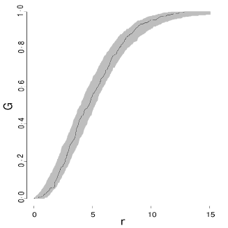
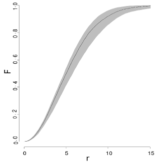
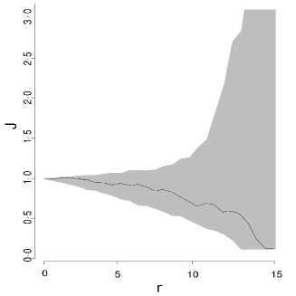
Parameter estimation based on $(\rho_{I},g_{I})$ and using a composite likelihood or a minimum contrast method is straightforward (Møller & Waagepetersen, 2007). Then, when checking a fitted Thomas process, we should not reuse the intensity and the pair correlation function. Below we use instead the functional summary statistics the empty space function $F$, the nearest-neighbour function $G$, and the $J$-function (Møller & Waagepetersen, 2004).

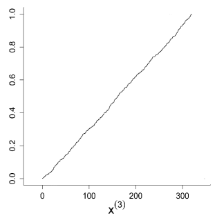
As an example, for the three-dimensional pyramidal cell data set in Figure 2 in accordance with the minicolumn hypothesis, we consider a degenerate Poisson line cluster point process. This has a columnar arrangement in the direction of the $x^{(3)}$-axis and the observation window is of the same form as described above with $D=[0,508]\times[0,138]$ and $I=[0,320]$. The first panel in Figure 5 shows the empirical cumulative distribution function of the $x^{(3)}$-coordinates of the pyramidal cell point pattern data set; there is no clear indication of a deviation from a uniform distribution, in agreement with our stationarity assumption.

When fitting the modified Thomas process for the projected point pattern onto $D$, for both composite likelihood and minimum contrast estimation, we used the spatstat (Baddeley & Turner, 2005) function kppm. We obtained the minimum contrast estimates $\hat{\rho}_{L}=0.024$, $\hat{\alpha}=0.37/320=0.0012$, and $\hat{\sigma}^{2}=15.04$, and similar estimates were obtained by a composite likelihood method. The three last panels in Figure 5 show the non-parametricly estimated $F$, $G$, and $J$-functions for the projected pyramidal cell point pattern onto $D$, together with $95\%$ simultaneous rank envelopes computed from 4999 simulated point patterns under the fitted Thomas process. The $p$-values for the rank envelope test (Myllymäki et al., 2016) for $G$, $F$, and $J$-functions are within the intervals $[0.851,0.852]$, $[0.732,0.733]$, and $[0.623,0.625]$, respectively, providing no evidence against the fitted model.

Figure 5: Summary statistics for the pyramidal cell point pattern data set: Empirical cumulative distribution function of the $x^{(3)}$-coordinates of the pyramidal cell point pattern data set (top left), and non-parametric estimates of $G$ (top right), $F$ (bottom left), and $J$ (bottom right) for the projected pyramidal cell point pattern onto $D$ (solid lines), together with $95\%$ simultaneous rank envelopes (gray regions) computed from 4999 simulated point patterns under the fitted Thomas process.

3.6 Bayesian inference

Suppose a non-empty realization $X_{W}=\{x_{1},\ldots,x_{n}\}$ is our data, where $W\subset\mathbb{R}^{d}$ is a bounded observation window, and we model $X$ as a Poisson line cluster point process with $k_{u^{\bot}}(y)=f(y\mid\sigma^{2})$ and $\mathcal{R}$ following the von Mises–Fisher density $f(u\mid\mu,\kappa)$ given by (9). As in Section 3.3 we need a finite representation $\Phi_{S}$ of $\Phi$ which we treat as a latent process. This section considers a Bayesian Markov chain Monte Carlo missing data approach for the missing data $\Phi_{S}$ and the unknown parameters $\rho_{L}>0$, $\mu\in\mathbb{S}^{d-1}$, $\kappa>0$, $\alpha>0$, and $\sigma^{2}>0$ .

Imagining that also a realization $\Phi_{S}=\{(y_{1},u_{1}),\ldots,(y_{k},u_{k})\}$ had been observed, we detail below the calculation of the likelihood $l[\rho_{L},\mu,\kappa,\alpha,\sigma^{2}\mid\{x_{1},\ldots,x_{n}\},\{(y_{1},u_{1}),\ldots,(y_{k},u_{k})\}]$. For the parameters, we assume independent prior densities $p(\rho_{L}),p(\mu),p(\kappa),p(\alpha),p(\sigma^{2})$; further prior specifications are given below. Hence the posterior density is

$$p[\rho_{L},\mu,\kappa,\alpha,\sigma^{2},\{(y_{1},u_{1}),\ldots,(y_{k},u_{k})\}\mid\{x_{1},\ldots,x_{n}\}]$$

$$\propto l[\rho_{L},\mu,\kappa,\alpha,\sigma^{2}\mid\{x_{1},\ldots,x_{n}\},\{(y_{1},u_{1}),\ldots,(y_{k},u_{k})\}]p(\rho_{L})p(\mu)p(\kappa)p(\alpha)p(\sigma^{2}).$$ (18)

As a first ingredient of the likelihood, using the approximation $\Phi_{S}$ of $\Phi$, we also approximate $X_{W}$ by a finite Cox process $X_{W,S}$ with driving random intensity function $\Lambda_{W}$ given by (10) with $k_{u^{\bot}}(\cdot)=f(\cdot\mid\sigma^{2})$. Conditional on $\Phi_{S}$, $X_{W,S}$ is absolutely continuous with respect to the unit rate Poisson process on $W$, with density

$$f[\{x_{1},\ldots,x_{n}\}\mid\Phi_{S},\alpha,\sigma^{2}]=\exp\left\{|W|-\int_{W}\Lambda_{W}(x\mid\Phi_{S},\alpha,\sigma^{2})\,\mathrm{d}x\right\}\prod_{i=1}^{n}\Lambda_{W}(x_{i}\mid\Phi_{S},\alpha,\sigma^{2})$$ (19)

for finite point configurations $\{x_{1},\ldots,x_{n}\}\subset W$.

For the second ingredient of the likelihood, notice that the distribution of $\Phi_{S}$ is absolutely continuous with respect to the distribution of a natural reference process $\Phi_{0,S}$ defined as the Poisson process on $S$ with intensity function $\chi_{0}(y,u)=|u^{(d)}|\Gamma(d/2)/(2\pi^{d/2})$ with respect to the measure $\lambda(\mathrm{d}y)\nu_{d-1}(\mathrm{d}u)$, cf. Section 3.3. This reference process corresponds to the case of an isotropic Poisson line process with unit intensity. The density of $\Phi_{S}$ with respect to the distribution of $\Phi_{0,S}$ is

$$f[\{(y_{1},u_{1}),\ldots,(y_{k},u_{k})\}\mid\rho_{L},\mu,\kappa]$$

$$=\exp\left[\int_{S}\left\{\chi_{0}(y,u)-\chi(y,u\mid\rho_{L},\mu,\kappa)\right\}\lambda(\mathrm{d}y)\nu_{d-1}(\mathrm{d}u)\right]\prod_{j=1}^{k}\frac{\chi(y_{j},u_{j}\mid\rho_{L},\mu,\kappa)}{\chi_{0}(y_{j},u_{j})}$$

for finite point configurations $\{(y_{1},u_{1}),\ldots,(y_{k},u_{k})\}\subset S$. That is, using the notation in Section 3.3,

$$f[\{(y_{1},u_{1}),\ldots,(y_{k},u_{k})\}\mid\rho_{L},\mu,\kappa]$$

$$\propto\exp\left\{-\rho_{L}I(\mu,\kappa)\right\}\prod_{j=1}^{k}\left\{\frac{2\pi^{d/2}}{\Gamma(d/2)}\rho_{L}f(u_{j}\mid\mu,\kappa)\mathbb{1}(y_{j}\in J_{u_{j}})\right\},$$ (20)

where we have omitted a constant not depending on the parameters.

Combining (19)–(20) we obtain the approximate likelihood

$$l[\rho_{L}, \mu,\kappa,\alpha,\sigma^{2}\mid\{x_{1},\ldots,x_{n}\},\{(y_{1},u_{1}),\ldots,(y_{k},u_{k})\}]$$

$$=\, \exp\left\{|W|-\int_{W}\Lambda_{W}(x\mid\Phi_{S},\alpha,\sigma^{2})\,\mathrm{d}x\right\}\prod_{i=1}^{n}\Lambda_{W}(x_{i}\mid\Phi_{S},\alpha,\sigma^{2})$$

$$\times\exp\left\{-\rho_{L}I(\mu,\kappa)\right\}\prod_{j=1}^{k}\left\{\frac{2\pi^{d/2}}{\Gamma(d/2)}\rho_{L}f(u_{j}\mid\mu,\kappa)\mathbb{1}(y_{j}\in J_{u_{j}})\right\}.$$ (21)

Inserting this into (18), we notice that the posterior density is analytically intractable. A hybrid Markov chain Monte Carlo algorithm or Metropolis within Gibbs algorithm, see e.g. Gilks et al. (1996), for posterior simulations is proposed in Appendix C. Briefly, the algorithm alternates between updating each of the parameters and the line process, using a birth-death-move Metropolis Hastings algorithm for the line process.

To illustrate the Bayesian approach we consider the two-dimensional chapel data set in the left panel of Figure 2, using a uniform prior for both $\mu=(\cos\varphi,\sin\varphi)$ and $\sigma^{2}$, and flat conjugated gamma priors for $\rho_{L}$ and $\alpha$, see Figure 6. Our posterior results for $\rho_{L}$, $\varphi$, and $\alpha$ were sensitive to the choice of prior distribution for $\kappa$. For small values of $\kappa$, i.e., values less than $30$, meaningless posterior results appeared, since $\varphi$ was approximately uniform, and for $\varphi$ close to zero, $\rho_{L}$ tended to zero and hence $\alpha$ tended to infinity. On the other hand, very large values of $\kappa$ caused a very concentrated posterior distribution for $\varphi$. As a compromise, after some experimentation, we fixed $\kappa=40$.

For this model an extension of the observation window $W=[-.5,.5]^{2}$ to $W_{\text{ext}}=[-0.55,0.55]^{2}$ seemed large enough to account for edge effects. For the posterior simulations we used 200,000 iterations, where one iteration consists of updating all the parameters and the missing data. We considered trace plots, which have been omitted here, for the parameters and information about the missing data, indicating that a burn-in of 5000 iterations is sufficient.

There is a clear distinction between the simulated posterior results for the parameters and the priors, cf. the first four panels in Figure 6. The posterior mean of $\varphi$ ($115.02^{\circ}$) is in close agreement with the result of $117^{\circ}$ found in Section 2.4, and $\sigma$ is unlikely to be larger than $0.02$, indicating that the points are rather close to the lines and that the choice of $W_{\mathrm{ext}}$ makes sense. The final panel in Figure 6 shows a good agreement between the number of chapels (110) and the posterior mean of the intensity $\rho$ (103.7), though there is some uncertainty in the posterior distribution of $\rho$. Moreover, the posterior means of $\rho_{L}$ and $\alpha$ are 12.9 and 8.4, respectively, which combined with (15) result in the estimate 108.4 for $\rho$.

Figure 6: Prior and posterior distributions: The first four panels show the unnormalized prior density (solid line) and histogram for the posterior distribution of $\rho_{L}$, $\varphi$, $\alpha$, and $\sigma^{2}$, respectively. The final panel shows the histogram for the posterior distribution of $\rho$.

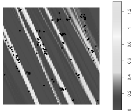
To illustrate the usefulness of the Bayesian method in detecting linear structures, Figure 7 shows a posterior kernel estimate of the density of lines within $W$. The estimate visualizes where the hidden lines could be, i.e., the lighter areas, and overall they agree with the point pattern of chapels, which is superimposed in the figure, though in the upper right corner of the observation window there is some doubt about whether there should be a single or two clusters of points. Specifically, the estimate is obtained from 100 posterior iterations with an equal spacing, and it is the average of binary pixel representations of the line process, where a pixel has value 1 if it is intersected by a line, and value 0 otherwise.

Figure 7: Posterior kernel estimate of the density of lines. For comparison, the chapel point pattern data set is superimposed.

4 Discussion

4.1 Choice of structuring element

Ripley’s $K$-function has a ball as structuring element but this is not useful for detecting anisotropy. Directional $K$-functions have been suggested using a sector annulus (Ohser & Stoyan, 1981) or a double cone (Redenbach et al., 2009) as the structuring element, while we have suggested a cylinder. Another suggestion could be an ellipsoid.

A detailed comparison of the cylindrical $K$-function with the $K$-function in Redenbach et al. (2009) using a double cone as the structuring element is given in a technical report by F. Safavimanesh and C. Redenbach from 2016. They conclude that in situations where the anisotropy is pronounced, a good choice of structuring element may be important and will depend on the application at hand. In case of geometric anisotropy (Møller & Toftaker, 2014), an ellipsoid is appropriate; when there is a columnar structure as under the Poisson line cluster point process model or in the data sets considered in this paper, an elongated cylinder is appropriate; while if regular point process models are compressed, then a double cone is appropriate. F. Safavimanesh and C. Redenbach emphasize the importance of an appropriate choice of the scale and shape parameters used to specify the structuring element, i.e. $r$ and $t$ in case of $K_{u}(r,t)$. They notice that prior information, e.g., the diameter of the clusters/mini-columns of points in case of the pyramidal cells (Rafati et al., 2016), can be used to determine interesting ranges of $r$ values.

4.2 Non-stationary case

In some applications it is relevant to use a non-constant intensity function $\rho(x)$. Suppose we assume second order intensity reweighted stationarity (Baddeley, Møller & Waagepetersen, 2000) and $g(x)$ still denotes the pair correlation function. This means intuitively, that if $x_{1},x_{2}\in\mathbb{R}^{d}$ are distinct locations and $B_{1},B_{2}$ are infinitesimally small sets of volumes $\mathrm{d}x_{1},\,\mathrm{d}x_{2}$ and containing $x_{1},x_{2}$, respectively, then $\rho(x_{1})\rho(x_{2})g(x_{1}-x_{2})\,\mathrm{d}x_{1}\,\mathrm{d}x_{2}$ is the probability for $X$ having a point in each of $B_{1}$ and $B_{2}$. Our definition (1) still applies, while (2) becomes

$$K_{u}(r,t)=\frac{1}{|W|}E\left[\sum_{x_{1},x_{2}\in X:\,x_{1}\not=x_{2}}\frac{\mathbb{1}\{x_{1}\in W,x_{2}-x_{1}\in C_{u}(r,t)\}}{\rho(x_{1})\rho(x_{2})}\right],\quad r>0,\ t>0,$$

which in turn can be used when deriving non-parametric estimates.

Assumption (B2) may be relaxed to obtain a non-stationary Poisson line cluster point process model for $X$, assuming that for each line $l_{i}$ the Poisson process $Q_{i}$ has intensity function $\alpha_{i}(x)=\alpha(x)$ for $x\in l_{i}$, where $\alpha$ is a non-negative function which is locally integrable on any line in $\mathbb{R}^{d}$. Then (6) should be replaced by

$$\Lambda(x)=\sum_{i=1}^{\infty}\alpha\{(x\cdot u_{i})u_{i}+y_{i}\}k_{u_{I}^{\bot}}\{p_{u_{i}^{\bot}}(x-y_{i})\},\quad x\in\mathbb{R}^{d}.$$ (22)

However, this non-stationary extension of the model will be harder to analyze, e.g., moment results as established in Section 3.4 for the stationary case will in general not easily extend, and it turns out that the model is not second order intensity reweighted stationary except in a special case discussed below. Moreover, while our statistical methodology in Section 3.4 can be straightforwardly extended, the Bayesian computations in Section 3.6 become harder.

In (22) assume that the intensity function $\alpha(y^{(1)},\ldots,y^{(d-1)},x^{(d)})=\alpha(x^{(d)})$ does not depend on $y=(y^{(d)},\ldots,y^{(d-1)},0)\in H$. Let $c=\int_{I}\alpha\{x^{(d)}\}\,\mathrm{d}x^{(d)}$. Then, using a notation as in Section 3.4, it can be shown that $X$ is second order intensity reweighted stationary, $X_{I}$ is still a Neyman–Scott process, while the $x^{(d)}$-coordinates of the points in $X_{W}$ are independent and identically distributed with density $\alpha\{x^{(d)}\}/c$, and they are independent of $X_{W}$. Therefore statistical inference simply splits into modelling the density $\alpha\{x^{(d)}\}/c$ based on the $x^{(d)}$-coordinates of the points in $X_{W}$ and inferring $(c,\rho_{L},\sigma^{2})$ by considering $X_{I}$ along similar lines as in Section 3.4 but with $\alpha\{x^{(d)}\}|I|$ replaced by $c$.

Acknowledgments

Supported by the Danish Council for Independent Research | Natural Sciences, and by the Centre for Stochastic Geometry and Advanced Bioimaging, funded by the Villum Foundation. We thank Jens Randel Nyengaard, Karl-Anton Dorph-Petersen, and Ali H. Rafati for collecting the three-dimensional pyramidal cell data set.

Appendix A: Intensity and rose of direction for a Poisson line process

First we give the definition of the intensity $\rho_{L}$ and the rose of direction $\mathcal{R}$ for a general stationary line process $L=\{l_{1},l_{2},\ldots\}$ in $\mathbb{R}^{d}$. Let $|\cdot|_{1}$ denote one-dimensional Lebesgue measure, $\mathrm{d}t$ Lebesgue measure on the real line, $A\subseteq\mathbb{R}^{d}$ an arbitrary Borel set with volume $|A|\in(0,\infty)$, and an $B\subseteq\mathbb{S}^{d-1}$ arbitrary Borel set. Then by definition and since $L$ is stationarity,

$$\rho_{L}=E\left(\sum_{i=1}^{\infty}|l_{i}\cap A|_{1}/|A|\right)$$ (23)

does not depend on the choice of $A$, and provided $0<\rho_{L}<\infty$,

$$\mathcal{R}(B)=E\left\{\sum_{i=1}^{\infty}|l_{i}\cap A|_{1}\mathrm{1}(u_{i}\in B)/\left(\rho_{L}|A|\right)\right\}$$ (24)

does not depend on the choice of $A$ and is seen to be a probability measure.

Second we assume that $L$ is a stationary Poisson line process as in Section 3.1. Then

$$E\left\{\sum_{i=1}^{\infty}|l_{i}\cap A|_{1}\mathrm{1}(u\in B)\right\}=\, E\left\{\sum_{i=1}^{\infty}\int\mathrm{1}(y_{i}+tu_{i}\in A,\,u_{i}\in B)\,\mathrm{d}t\right\}$$ (25)

$$\ =\, \beta\int\int\int\mathrm{1}(y+tu\in A,\,u\in B)\,\mathrm{d}t\,\lambda(\mathrm{d}y)\,M(\mathrm{d}u)$$ (26)

$$=\, \beta|A|\int_{B}1/|u^{(d)}|\,M(\mathrm{d}u).$$ (27)

Here (25) follows from the phase representation of $L$ (see Section 3.1), (26) from the Slivnyak–Mecke theorem for the Poisson process $\Phi$ (see e.g. Møller & Waagepetersen (2004)), and (27) since $|u^{(d)}|$ is the Jacobian of the mapping $(t,y)\mapsto y+tu$ with $(t,y)\in\mathbb{R}\times H$. When $B=\mathbb{S}^{d-1}$ we obtain from (23) and (27) the first equation in (7). This together with $0<\beta<\infty$ and $0<\int_{\mathbb{S}^{d-1}}1/|u^{(d)}|\,M(\mathrm{d}u)<\infty$ imply that $0<\rho_{L}<\infty$. Thereby the second first equation in (7) follows for any Borel set $B\subseteq\mathbb{S}^{d-1}$.

Appendix B: Moment results for a Poisson line cluster point process

For Section 3.4 it remains to verify (15)–(16).

Proof of (15): By (6), (14), and the Slivnyak–Mecke theorem for the Poisson process,

$$\rho=\alpha\beta\int\int k_{u}\{-p_{u}(y)\}\,\lambda(\mathrm{d}y)\,M(\mathrm{d}u).$$ (28)

Let $I_{d}$ be the $d\times d$ identity matrix, and $o_{d-1}$ the origin in $\mathbb{R}^{d-1}$. For $u\in\mathbb{S}^{d-1}$, let $A(u)=vv^{T}$ where $v$ is the subvector consisting of the first $d-1$ coordinates of $u$ and ^T denotes transpose of a vector or matrix. The Jacobian of the linear transformation

$$p_{u}(y)=\left(I_{d}-uu^{T}\right)y,\quad y\in H,$$

is the square root of the determinant of the $(d-1)\times(d-1)$ matrix

$$Q =\left\{\left(I_{d}-uu^{T}\right)\left(I_{d-1}\ o_{d-1}\right)^{T}\right\}^{T}\left(I_{d}-uu^{T}\right)\left(I_{d-1}\ o_{d-1}\right)^{T}$$

$$=\left(I_{d-1}\ o_{d-1}\right)\left(I_{d}-uu^{T}\right)\left(I_{d-1}\ o_{d-1}\right)^{T}$$

$$=I_{d-1}-A(u).$$

Since $A(u)$ is symmetric of rank at most one and has trace $\mbox{tr}\{A(u)\}=\{u^{(1)}\}^{2}+\ldots+\{u^{(d-1)}\}^{2}=1-\{u^{(d)}\}^{2}$, the determinant of $Q$ is $1-\mbox{tr}\{A(u)\}=\{u^{(d)}\}^{2}$. Combining this with (28) we obtain

$$\rho=\alpha\beta\int\int k_{u}(-y)/|u^{(d)}|\,\lambda_{u}(\mathrm{d}y)\,M(\mathrm{d}u).$$

Thereby (15) easily follows from the first identity in (7).

Proof of (16): By (6) and (14),

$$\rho^{2}g(x) =\alpha^{2}E\left[\sum_{i\not=j}k_{u_{i}^{\bot}}\{p_{u_{i}^{\bot}}(-y_{i})\}k_{u_{j}^{\bot}}\{p_{u_{j}^{\bot}}(x-y_{j})\}\right]$$

$$+\alpha^{2}E\left[\sum_{i}k_{u_{i}^{\bot}}\{p_{u_{i}^{\bot}}(-y_{i})\}k_{u_{i}^{\bot}}\{p_{u_{i}^{\bot}}(x-y_{i})\}\right]$$

$$=\rho^{2}+\alpha^{2}\beta\int k_{u^{\bot}}\{p_{u^{\bot}}(-y)\}k_{u^{\bot}}\{p_{u^{\bot}}(x-y)\}\,\lambda(\mathrm{d}y)\,M(\mathrm{d}u)$$ (29)

using the extended Slivnyak–Mecke theorem for the Poisson process and the proof of (15) to obtain that the first expectation is equal to $\rho^{2}$, and the Slivnyak–Mecke theorem for the Poisson process to obtain that the second expectation is equal to the last term. Combining (15) and (29) with the result for the Jacobian considered above, we obtain (16).

Appendix C: Hybrid Markov chain Monte Carlo algorithm

This appendix details the Markov chain Monte Carlo algorithm for the Bayesian approach considered in Section 3.6, with independent prior densities for the parameters and posterior density given by (18)–(21). As in Section 3.6, we consider conjugated gamma densities $p(\alpha)$ and $p(\rho_{L})$, and denote their shape parameters by $a_{1}$ and $a_{2}$ and their inverse scale parameters by $b_{1}$ and $b_{2}$, respectively. The remaining parameters have no (well-known) conjugate priors, cf. (19) and (20), and thus we consider generic prior densities $p(\mu)$, $p(\kappa)$, and $p(\sigma^{2})$.

In each iteration of the Markov chain Monte Carlo algorithm we update first each of the parameters and second the missing data. We use a Gibbs update for $\alpha$ respective $\rho_{L}$, noting that the conditional distribution of $\alpha$ given the rest is a gamma distribution with shape parameter $a_{1}+n$ and inverse scale parameter $b_{1}+\int_{W}\sum_{j=1}^{k}f\{p_{u_{j}^{\bot}}(x-y_{j})\mid\sigma^{2}\}\,\mathrm{d}x$, and the conditional distribution of $\rho_{L}$ given the rest is a gamma distribution with shape parameter $a_{2}+k$ and inverse scale parameter $b_{2}+I(\mu,\kappa)$. Below we describe the individual proposals and Hastings ratios for the remaining parameters and the missing data (in the case of Section 3.6 where the value of $\kappa$ is fixed, we can of course just ignore the update of $\kappa$ described below). As usual, for each type of update, the proposal is accepted with probability $\min\{1,R\}$, where $R$ is the corresponding Hastings ratio. We denote $(\rho_{L},\mu,\kappa,\alpha,\sigma^{2},\{(y_{1},u_{1}),\ldots,(y_{k},u_{k})\})$ the current state of the algorithm, where $n\geq 1$, $k\geq 1$ (since $k=0$ implies $n=0$, which is not a case of interest), and $l(y_{i},u_{i})\cap W_{\text{ext}}\not=\emptyset,i=1,\ldots,k$.

For $\mu$, $\kappa$, and $\sigma^{2}$, we use Metropolis random walk updates, with a von Mises–Fisher proposal $\mu^{\prime}\sim f(\cdot\mid\mu,\kappa_{0})$ and normal proposals $\kappa^{\prime}\sim N(\kappa,\sigma_{0,1}^{2})$ and $\sigma^{\prime 2}\sim N(\sigma^{2},\sigma_{0,2}^{2})$, where $\kappa_{0},\sigma_{0,1}^{2},\sigma_{0,2}^{2}>0$ are tuned so that the mean acceptance probabilities are between 20–45% (as recommended in Roberts, Gelman & Gilks (1997)). The Hastings ratios for the acceptance probabilities are

$$R_{\mu}=\frac{p(\mu^{\prime})}{p(\mu)}\exp\left[\rho_{L}\left\{I(\mu,\kappa)-I(\mu^{\prime},\kappa)\right\}\right]\prod_{j=1}^{k}\frac{f(u_{j}\mid\mu^{\prime},\kappa)}{f(u_{j}\mid\mu,\kappa)},$$

$$R_{\kappa}=\mathbb{1}(\kappa^{\prime}>0)\frac{p(\kappa^{\prime})}{p(\kappa)}\exp\left[\rho_{L}\left\{I(\mu,\kappa)-I(\mu,\kappa^{\prime})\right\}\right]\prod_{j=1}^{k}\frac{f(u_{j}\mid\mu,\kappa^{\prime})}{f(u_{j}\mid\mu,\kappa)},$$

and

$$R_{\sigma^{2}}= \,\mathbb{1}(\sigma^{\prime 2}>0)\frac{p(\sigma^{\prime 2})}{p(\sigma^{2})}\exp\Bigg{(}\alpha\sum_{j=1}^{k}\left[\int_{W}f\{p_{u_{j}^{\bot}}(x-y_{j})\mid\sigma^{2}\}\,\mathrm{d}x\right.$$

$$\left.-\int_{W}f\{p_{u_{j}^{\bot}}(x-y_{j})\mid\sigma^{\prime 2}\}\,\mathrm{d}x\right]\Bigg{)}\prod_{i=1}^{n}\frac{\sum_{j=1}^{k}f\{p_{u_{j}^{\bot}}(x_{i}-y_{j})\mid\sigma^{\prime 2}\}}{\sum_{j=1}^{k}f\{p_{u_{j}^{\bot}}(x_{i}-y_{j})\mid\sigma^{2}\}}.$$

For $R_{\sigma^{2}}$ each integral is calculated by a simple Monte Carlo method after making a change of variables from $x$ to its Cartesian coordinates in a system centered at $y_{j}$ and with axes given by $u_{j}$ and $u_{j}^{\bot}$.

For the missing data, we adapt the birth-death-move Metropolis-Hastings algorithm in Geyer & Møller (1994) as follows. Each of the birth/death/move proposals happens with probability $1/3$ and consists of the following action. A birth proposal is the proposal of adding a new point $(y,u)$, where $u\sim f(\cdot\mid\mu,\kappa)$ and $y$ conditional on $u$ is uniformly distributed on $J_{u}$. Then, as explained below, the Hastings ratio is

$$R_{\text{birth}}= \,\frac{\rho_{L}\lambda(J_{u})|u^{(d)}|}{k+1}\mathbb{1}\{l(y,u)\cap W_{\text{ext}}\not=\emptyset\}$$

$$\times\exp\left[-\alpha\int_{W}f\{p_{u^{\bot}}(x-y)\mid\sigma^{2}\}\mathrm{d}x\right]\prod_{i=1}^{n}\left[1+\frac{f\{p_{u^{\bot}}(x_{i}-y)\mid\sigma^{2}\}}{\sum_{j=1}^{k}f\{p_{u_{j}^{\bot}}(x_{i}-y_{j})\mid\sigma^{2}\}}\right].$$ (30)

To stress the dependence on $\{(y_{1},u_{1}),\ldots,(y_{k},u_{k})\}$ and $(y,u)$, write $R_{\text{birth}}=R_{\text{birth}}(y_{1},u_{1},\ldots,y_{k},u_{k};y,u)$ (obviously, it also depends on $\rho_{L},\alpha,\sigma^{2}$, and $\{x_{1},\ldots,x_{n}\}$). A death proposal is the proposal of generating a uniform $j\in\{1,\ldots,k\}$ (provided $k>1$; if $k=1$, we do nothing and keep the current state) and deleting $(y_{j},u_{j})$. Then, as explained below, the Hastings ratio is

$$R_{\text{death}}=1/R_{\text{birth}}(y_{1},u_{1},\ldots,y_{j-1},u_{j-1},y_{j+1},u_{j+1}\ldots,y_{k},u_{k};y_{j},u_{j}).$$ (31)

Finally, a move proposal is the proposal of selecting a uniform $j\in\{1,\ldots,k\}$ and replacing $(y_{j},u_{j})$ by $(y^{\prime}_{j},u^{\prime}_{j})$, where $u^{\prime}_{j}\sim f(\cdot\mid\mu,\kappa)$ and $y^{\prime}_{j}$ conditional on $u^{\prime}_{j}$ is uniformly distributed on $J_{u^{\prime}_{j}}$. Since this can be considered as first a death proposal and second a birth proposal, the Hastings ratio is

$$R_{\text{move}}=\frac{R_{\text{birth}}(y_{1},u_{1},\ldots,y_{j-1},u_{j-1},y_{j+1},u_{j+1}\ldots,y_{k},u_{k};y^{\prime}_{j},u^{\prime}_{j})}{R_{\text{birth}}(y_{1},u_{1},\ldots,y_{j-1},u_{j-1},y_{j+1},u_{j+1}\ldots,y_{k},u_{k};y_{j},u_{j})}.$$

It remains to explain how we obtained the Hastings ratios (Appendix C: Hybrid Markov chain Monte Carlo algorithm)–(31), where we notice the following facts. The reference Poisson process $\Phi_{0,S}$ has intensity measure

$$\zeta(\mathrm{d}y,\mathrm{d}u)=|u^{(d)}|\frac{\Gamma(d/2)}{2\pi^{d/2}}\lambda(\mathrm{d}y)\nu_{d-1}(\mathrm{d}u).$$

Further, conditional on the data $X_{W}=\{x_{1},\ldots,x_{n}\}$ and the parameters $\rho_{L}$, $\mu$, $\kappa$, $\alpha$, $\sigma^{2}$, the target process $\Phi_{S}$ has density

$$f[\{(y_{1},u_{1}),\ldots,(y_{k},u_{k})\}\mid\{x_{1},\ldots,x_{n}\},\alpha,{\sigma}^{2},\rho_{L},\mu,\kappa]$$

$$\propto f[\{x_{1},\ldots,x_{n}\}\mid\{(y_{1},u_{1}),\ldots,(y_{k},u_{k})\},\alpha,\sigma^{2}]f[\{(y_{1},u_{1}),\ldots,(y_{k},u_{k})\}\mid\rho_{L},\mu,\kappa]$$

with respect to the distribution of $\Phi_{0,S}$. Furthermore, if a birth $(y,u)$ is proposed, then it has density

$$f(y,u\mid\mu,\kappa)=\frac{f(u\mid\mu,\kappa)\mathbb{1}(y\in J_{u})/\lambda(J_{u})}{|u^{(d)}|\Gamma(d/2)/(2\pi^{d/2})}$$

with respect to $\zeta$. Consequently, by Geyer & Møller (1994), the Hastings ratio for the proposed birth is

$$R_{\text{birth}}= \,\frac{f[\{(y_{1},u_{1}),\ldots,(y_{k},u_{k}),(y,u)\}\mid\{x_{1},\ldots,x_{n}\},\alpha,{\sigma}^{2},\rho_{L},\mu,\kappa]}{f[\{(y_{1},u_{1}),\ldots,(y_{k},u_{k})\}\mid\{x_{1},\ldots,x_{n}\},\alpha,{\sigma}^{2},\rho_{L},\mu,\kappa]}\times\frac{1/(k+1)}{f(y,u\mid\mu,\kappa)}$$

$$= \,\frac{2\pi^{d/2}}{\Gamma(d/2)}\rho_{L}f(u\mid\mu,\kappa)\mathbb{1}(y\in J_{u})\frac{1}{(k+1)f(y,u\mid\mu,\kappa)}$$

$$\times\exp\left[-\alpha\int_{W}f\{p_{u^{\bot}}(x-y)\mid\sigma^{2}\}\mathrm{d}x\right]\prod_{i=1}^{n}\left[1+\frac{f\{p_{u^{\bot}}(x_{i}-y)\mid\sigma^{2}\}}{\sum_{j=1}^{k}f\{p_{u_{j}^{\bot}}(x_{i}-y_{j})\mid\sigma^{2}\}}\right]$$

which is equal to (Appendix C: Hybrid Markov chain Monte Carlo algorithm). Thereby, refering again to Geyer & Møller (1994), we obtain (31).

References

• Baddeley et al. (2000) Baddeley, A., Møller, J. & Waagepetersen, R. (2000). Non- and semi-parametric estimation of interaction in inhomogeneous point patterns. Statistica Neerlandica 54, 329–350.
• Baddeley & Turner (2005) Baddeley, A. & Turner, R. (2005). Spatstat: an R package for analyzing spatial point patterns. Journal of Statistical Software 12, 1–42.
• Chiu et al. (2013) Chiu, S. N., Stoyan, D., Kendall, W. S. & Mecke, J. (2013). Stochastic Geometry and Its Applications. John Wiley and Sons, Chichester, 3rd ed.
• Diggle et al. (1995) Diggle, P. J., Chetwynd, A., Häggkvist, R. & Morris, S. (1995). Second order analysis of space-time clustering. Statistical Methods in Medical Research 4, 124–136.
• Diggle & Gratton (1984) Diggle, P. J. & Gratton, R. (1984). Monte Carlo methods of inference for implicit statistical models (with discussion). Journal of the Royal Statistical Society: Series B (Statistical Methodology) 46, 193–212.
• Gabriel & Diggle (2009) Gabriel, E. & Diggle, P. J. (2009). Second-order analysis of inhomogeneous spatio-temporal point process data. Statistica Neerlandica 63, 43–51.
• Geyer & Møller (1994) Geyer, C. & Møller, J. (1994). Simulation procedures and likelihood inference for spatial point processes. Scandinavian Journal of Statistics 21, 359–373.
• Gilks et al. (1996) Gilks, W. R., Richardson, S. & Spiegelhalter, D. J. (1996). Markov Chain Monte Carlo in Practice. Chapman and Hall, London.
• Guan (2006) Guan, Y. (2006). A composite likelihood approach in fitting spatial point process models. Journal of the American Statistical Association 101, 1502–1512.
• Guan et al. (2006) Guan, Y., Sherman, M. & Calvin, J. A. (2006). Assessing isotropy for spatial point processes. Biometrics 62, 119–125.
• Illian et al. (2008) Illian, J., Penttinen, A., Stoyan, H. & Stoyan, D. (2008). Statistical Analysis and Modelling of Spatial Point Patterns. John Wiley and Sons, New York.
• Møller & Toftaker (2014) Møller, J. & Toftaker, H. (2014). Geometric anisotropic spatial point pattern analysis and Cox processes. Scandinavian Journal of Statistics 41, 414–435.
• Møller & Waagepetersen (2004) Møller, J. & Waagepetersen, R. (2004). Statistical Inference and Simulation for Spatial Point Processes. Chapman and Hall/CRC, Boca Raton.
• Møller & Waagepetersen (2007) Møller, J. & Waagepetersen, R. (2007). Modern statistics for spatial point processes (with discussion). Scandinavian journal of Statistics 34, 643–711.
• Møller & Waagepetersen (2016) Møller, J. & Waagepetersen, R. (2016). Some recent developments in statistics for spatial point pattern analysis. Annual Review of Statistics and Its Application (submitted invited paper).
• Mountcastle (1957) Mountcastle, V. B. (1957). Modality and topographic properties of single neurons of cat’s somatic sensory cortex. Journal of Neurophysiology 20, 408–434.
• Mugglestone & Renshaw (1996) Mugglestone, M. & Renshaw, E. (1996). A practical guide to the spectral analysis of spatial point processes. Computational Statistics &\& Data Analysis 21, 43–65.
• Myllymäki et al. (2016) Myllymäki, M., Mrkvička, T., Seijo, H. & Grabarnik, P. (2016). Global envelope tests for spatial processes. Journal of the Royal Statistical Society: Series B (Statistical Methodology) (to appear).
• Nicolis et al. (2010) Nicolis, O., Mateu, J. & D’Ercole, R. (2010). Testing for anisotropy in spatial point processes. In Proceedings of the Fifth International Workshop on Spatio-Temporal Modelling (METMA5), G.-M. et al., ed. Unidixital, Santiago de Compostela.
• Ohser & Stoyan (1981) Ohser, J. & Stoyan, D. (1981). On the second-order and orientation analysis of planar stationary point processes. Biometrical Journal 23, 523–533.
• Rafati et al. (2016) Rafati, A., Safavimanesh, F., Dorph-Petersen, K., Rasmussen, J. G., Møller, J. & Nyengaard, J. R. (2016). Detection and spatial characterization of minicolumnarity in the human cerebral cortex. Journal of Microscopy 261, 115–126.
• Redenbach et al. (2009) Redenbach, C., Särkkä, A., Freitag, J. & Schladitz, K. (2009). Anisotropy analysis of pressed point processes. Advances in Statistical Analysis 93, 237–261.
• Ripley (1976) Ripley, B. D. (1976). The second-order analysis of stationary point processes. Journal of Applied Probability 13, 255–266.
• Ripley (1977) Ripley, B. D. (1977). Modelling spatial patterns (with discussion). Journal of the Royal Statistical Society: Series B (Statistical Methodology) 39, 172–212.
• Roberts et al. (1997) Roberts, G. O., Gelman, A. & Gilks, W. R. (1997). Weak convergence and optimal scaling of random walk Metropolis algorithms. Annual of Applied Probability 7, 110–120.
• Rosenberg (2004) Rosenberg, M. S. (2004). Wavelet analysis for detecting anisotropy in point patterns. Journal of Vegetation Science 15, 277–284.
• Stoyan (1991) Stoyan, D. (1991). Describing the anisotropy of marked planer point process. Statistics: A Journal of Theoretical and Applied Statistics 22, 449–462.
• Stoyan & Beneš (1991) Stoyan, D. & Beneš, V. (1991). Anisotropy analysis for particle systems. Journal of Microscopy 164, 159–168.
• Stoyan & Stoyan (1995) Stoyan, D. & Stoyan, H. (1995). Fractals, Random Shapes and Point Fields. John Wiley and Sons, Chichester.