The extended oloid and its inscribed quadrics

Uwe Bäsel and Hans Dirnböck
Abstract

The oloid is the convex hull of two circles with equal radius in perpendicular planes so that the center of each circle lies on the other circle. It is part of a developable surface which we call extended oloid. We determine the tangential system of all inscribed quadrics 𝒬λsubscript𝒬𝜆\mathcal{Q}_{\lambda} of the extended oloid 𝒪𝒪\mathcal{O} where λ𝜆\lambda is the system parameter. From this result we conclude parameter equations of the touching curve 𝒞λsubscript𝒞𝜆\mathcal{C}_{\lambda} between 𝒪𝒪\mathcal{O} and 𝒬λsubscript𝒬𝜆\mathcal{Q}_{\lambda}, the edge of regression \mathcal{R} of 𝒪𝒪\mathcal{O}, and the asymptotes of \mathcal{R}. Properties of the curves 𝒞λsubscript𝒞𝜆\mathcal{C}_{\lambda} are investigated, including the case that λ±𝜆plus-or-minus\lambda\rightarrow\pm\infty. The self-polar tetrahedron of the tangential system 𝒬λsubscript𝒬𝜆\mathcal{Q}_{\lambda} is obtained. The common generating lines of 𝒪𝒪\mathcal{O} and any ruled surface 𝒬λsubscript𝒬𝜆\mathcal{Q}_{\lambda} are determined. Furthermore, we derive the curves which are the images of 𝒞λsubscript𝒞𝜆\mathcal{C}_{\lambda} and \mathcal{R} when 𝒪𝒪\mathcal{O} is developed onto the plane.
Mathematics Subject Classification: 51N05, 53A05
Keywords: oloid, extended oloid, developable, tangential system of quadrics, touching curve, edge of regression, self-polar tetrahedron, ruled surface

1 Introduction

The oloid was discovered by Paul Schatz in 1929. It is the convex hull of two circles with equal radius r𝑟r in perpendicular planes so that the center of each circle lies on the other circle. The oloid has the remarkable properties that it develops its entire surface while rolling, and its surface area is equal to 4πr24𝜋superscript𝑟24\pi r^{2}. The surface of the oloid is part of a developable surface. [2], [8]
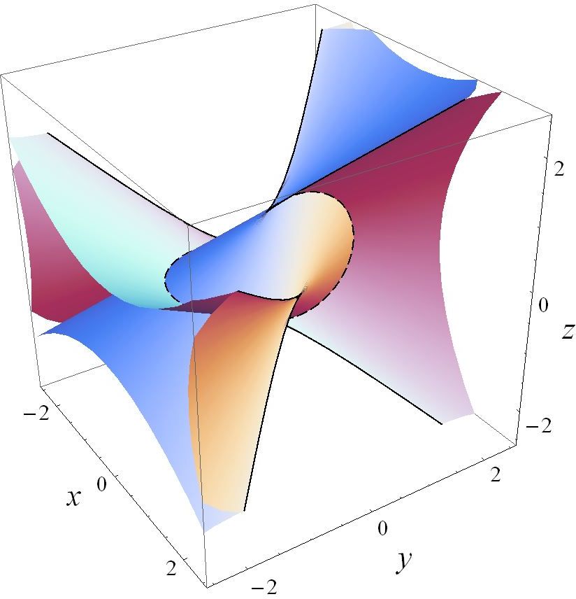
Refer to caption
Fig. 1: The extended oloid 𝒪𝒪\mathcal{O}, the circles kAsubscript𝑘𝐴k_{A}, kBsubscript𝑘𝐵k_{B} (dashed lines), and the edge of regression \mathcal{R} (solid lines) in the box 2.5x,y,z2.5formulae-sequence2.5𝑥𝑦𝑧2.5-2.5\leq x,y,z\leq 2.5

In the following this developable surface is called extended oloid. According to [2, pp. 105-106], with r=1𝑟1r=1 the circles can be defined by

kA:=assignsubscript𝑘𝐴absent\displaystyle k_{A}:={} {(x,y,z)3|x2+(y+12)2=1z=0},conditional-set𝑥𝑦𝑧superscript3superscript𝑥2superscript𝑦1221𝑧0\displaystyle\left\{(x,y,z)\in\mathbb{R}^{3}\;\big{|}\;x^{2}+\left(y+\tfrac{1}{2}\right)^{2}=1\wedge z=0\right\},
kB:=assignsubscript𝑘𝐵absent\displaystyle k_{B}:={} {(x,y,z)3|(y12)2+z2=1x=0}.conditional-set𝑥𝑦𝑧superscript3superscript𝑦122superscript𝑧21𝑥0\displaystyle\left\{(x,y,z)\in\mathbb{R}^{3}\;\big{|}\,\left(y-\tfrac{1}{2}\right)^{2}+z^{2}=1\wedge x=0\right\}.

In this case we denote the extended oloid by 𝒪𝒪\mathcal{O} (see Fig. 1).

Now we introduce homogeneous coordinates x0,x1,x2,x3subscript𝑥0subscript𝑥1subscript𝑥2subscript𝑥3x_{0},x_{1},x_{2},x_{3} with

x=x1x0,y=x2x0,z=x3x0.formulae-sequence𝑥subscript𝑥1subscript𝑥0formulae-sequence𝑦subscript𝑥2subscript𝑥0𝑧subscript𝑥3subscript𝑥0x=\frac{x_{1}}{x_{0}}\,,\quad y=\frac{x_{2}}{x_{0}}\,,\quad z=\frac{x_{3}}{x_{0}}\,.

Then the real projective space is given by

3()={[x0,x1,x2,x3](x0,x1,x2,x3)4{0}},subscript3conditional-setsubscript𝑥0subscript𝑥1subscript𝑥2subscript𝑥3subscript𝑥0subscript𝑥1subscript𝑥2subscript𝑥3superscript40\mathbb{P}_{3}(\mathbb{R})=\left\{[x_{0},x_{1},x_{2},x_{3}]\mid(x_{0},x_{1},x_{2},x_{3})\in\mathbb{R}^{4}\setminus\{0\}\right\},

where [x0,x1,x2,x3]=[y0,y1,y2,y3]subscript𝑥0subscript𝑥1subscript𝑥2subscript𝑥3subscript𝑦0subscript𝑦1subscript𝑦2subscript𝑦3[x_{0},x_{1},x_{2},x_{3}]=[y_{0},y_{1},y_{2},y_{3}] if there exist a μ{0}𝜇0\mu\in\mathbb{R}\setminus\{0\} such that xj=μyjsubscript𝑥𝑗𝜇subscript𝑦𝑗x_{j}=\mu y_{j} for j=1,2,3𝑗123j=1,2,3. Should it prove necessary, complex coordinates will be used instead of the real ones. For the description of the corresponding projective circles 𝒦Asubscript𝒦𝐴\mathcal{K}_{A} and 𝒦Bsubscript𝒦𝐵\mathcal{K}_{B} to kAsubscript𝑘𝐴k_{A} and kBsubscript𝑘𝐵k_{B}, respectively, we write

𝒦A:=assignsubscript𝒦𝐴absent\displaystyle\mathcal{K}_{A}:={} {[x0,x1,x2,x3]3()|φA(x0,x1,x2,x3)=0x3=0},conditional-setsubscript𝑥0subscript𝑥1subscript𝑥2subscript𝑥3subscript3subscript𝜑𝐴subscript𝑥0subscript𝑥1subscript𝑥2subscript𝑥30subscript𝑥30\displaystyle\left\{[x_{0},x_{1},x_{2},x_{3}]\in\mathbb{P}_{3}(\mathbb{R})\;\big{|}\;\varphi_{A}(x_{0},x_{1},x_{2},x_{3})=0\wedge x_{3}=0\right\},
𝒦B:=assignsubscript𝒦𝐵absent\displaystyle\mathcal{K}_{B}:={} {[x0,x1,x2,x3]3()|φB(x0,x1,x2,x3)=0x1=0}conditional-setsubscript𝑥0subscript𝑥1subscript𝑥2subscript𝑥3subscript3subscript𝜑𝐵subscript𝑥0subscript𝑥1subscript𝑥2subscript𝑥30subscript𝑥10\displaystyle\left\{[x_{0},x_{1},x_{2},x_{3}]\in\mathbb{P}_{3}(\mathbb{R})\;\big{|}\;\varphi_{B}(x_{0},x_{1},x_{2},x_{3})=0\wedge x_{1}=0\right\}

with

φA(x0,x1,x2,x3)=subscript𝜑𝐴subscript𝑥0subscript𝑥1subscript𝑥2subscript𝑥3absent\displaystyle\varphi_{A}(x_{0},x_{1},x_{2},x_{3})={} 3x024x0x24x124x22,3superscriptsubscript𝑥024subscript𝑥0subscript𝑥24superscriptsubscript𝑥124superscriptsubscript𝑥22\displaystyle 3x_{0}^{2}-4x_{0}x_{2}-4x_{1}^{2}-4x_{2}^{2}\,,
φB(x0,x1,x2,x3)=subscript𝜑𝐵subscript𝑥0subscript𝑥1subscript𝑥2subscript𝑥3absent\displaystyle\varphi_{B}(x_{0},x_{1},x_{2},x_{3})={} 3x02+4x0x24x224x32.3superscriptsubscript𝑥024subscript𝑥0subscript𝑥24superscriptsubscript𝑥224superscriptsubscript𝑥32\displaystyle 3x_{0}^{2}+4x_{0}x_{2}-4x_{2}^{2}-4x_{3}^{2}\,.

2 Inscribed quadrics

Lemma 1.

The dual figures to 𝒦Asubscript𝒦𝐴\mathcal{K}_{A} and 𝒦Bsubscript𝒦𝐵\mathcal{K}_{B} are

𝒦^A=subscript^𝒦𝐴absent\displaystyle\widehat{\mathcal{K}}_{A}={} {[u0,u1,u2,u3]3()| 4u024u0u24u123u22=0}andconditional-setsubscript𝑢0subscript𝑢1subscript𝑢2subscript𝑢3subscript34superscriptsubscript𝑢024subscript𝑢0subscript𝑢24superscriptsubscript𝑢123superscriptsubscript𝑢220and\displaystyle\left\{[u_{0},u_{1},u_{2},u_{3}]\in\mathbb{P}_{3}(\mathbb{R})\;\big{|}\;4u_{0}^{2}-4u_{0}u_{2}-4u_{1}^{2}-3u_{2}^{2}=0\right\}\quad\mbox{and}
𝒦^B=subscript^𝒦𝐵absent\displaystyle\widehat{\mathcal{K}}_{B}={} {[u0,u1,u2,u3]3()| 4u02+4u0u23u224u32=0},conditional-setsubscript𝑢0subscript𝑢1subscript𝑢2subscript𝑢3subscript34superscriptsubscript𝑢024subscript𝑢0subscript𝑢23superscriptsubscript𝑢224superscriptsubscript𝑢320\displaystyle\left\{[u_{0},u_{1},u_{2},u_{3}]\in\mathbb{P}_{3}(\mathbb{R})\;\big{|}\;4u_{0}^{2}+4u_{0}u_{2}-3u_{2}^{2}-4u_{3}^{2}=0\right\},

respectively, where u0,u1,u2,u3subscript𝑢0subscript𝑢1subscript𝑢2subscript𝑢3u_{0},u_{1},u_{2},u_{3} are homogeneous plane-coordinates. 𝒦^Asubscript^𝒦𝐴\widehat{\mathcal{K}}_{A} and 𝒦^Bsubscript^𝒦𝐵\widehat{\mathcal{K}}_{B} are elliptic cylinders. Their respective non homogeneous equations are

u2(23)2+(v+23)2(43)2=1<w<,\frac{u^{2}}{\left(\frac{2}{\sqrt{3}}\right)^{2}}+\frac{\left(v+\frac{2}{3}\right)^{2}}{\left(\frac{4}{3}\right)^{2}}=1\;\wedge\;-\infty<w<\infty\,,

and

<u<(v23)2(43)2+w2(23)2=1.𝑢superscript𝑣232superscript432superscript𝑤2superscript2321-\infty<u<\infty\;\wedge\;\frac{\left(v-\frac{2}{3}\right)^{2}}{\left(\frac{4}{3}\right)^{2}}+\frac{w^{2}}{\left(\frac{2}{\sqrt{3}}\right)^{2}}=1\,.
Proof.

Following [3, pp. 41-42], [4, pp. 160, 164-165], we determine 𝒦^Asubscript^𝒦𝐴\widehat{\mathcal{K}}_{A}. With

μui=φAxi,i{0,1,2,3},formulae-sequence𝜇subscript𝑢𝑖subscript𝜑𝐴subscript𝑥𝑖𝑖0123\mu u_{i}=\frac{\partial\varphi_{A}}{\partial x_{i}}\,,\quad i\in\{0,1,2,3\}\,,

we get

μu0=6x04x2,μu1=8x1,μu2=4x08x2,μu3=0.formulae-sequence𝜇subscript𝑢06subscript𝑥04subscript𝑥2formulae-sequence𝜇subscript𝑢18subscript𝑥1formulae-sequence𝜇subscript𝑢24subscript𝑥08subscript𝑥2𝜇subscript𝑢30\mu u_{0}=6x_{0}-4x_{2}\,,\quad\mu u_{1}=-8x_{1}\,,\quad\mu u_{2}=-4x_{0}-8x_{2}\,,\quad\mu u_{3}=0\,.

Solving this system of linear equations for x0subscript𝑥0x_{0}, x1subscript𝑥1x_{1}, x2subscript𝑥2x_{2} delivers

x0=μ(18u0116u2),x1=μ(18u1),x2=μ(116u0332u2).formulae-sequencesubscript𝑥0𝜇18subscript𝑢0116subscript𝑢2formulae-sequencesubscript𝑥1𝜇18subscript𝑢1subscript𝑥2𝜇116subscript𝑢0332subscript𝑢2x_{0}=\mu\left(\frac{1}{8}\,u_{0}-\frac{1}{16}\,u_{2}\right),\quad x_{1}=\mu\left(-\frac{1}{8}\,u_{1}\right),\quad x_{2}=\mu\left(-\frac{1}{16}\,u_{0}-\frac{3}{32}\,u_{2}\right).

So we get

0=u0x0+u1x1+u2x2+u3x3=132μ(4u024u0u24u123u22);0subscript𝑢0subscript𝑥0subscript𝑢1subscript𝑥1subscript𝑢2subscript𝑥2subscript𝑢3subscript𝑥3132𝜇4superscriptsubscript𝑢024subscript𝑢0subscript𝑢24superscriptsubscript𝑢123superscriptsubscript𝑢220=u_{0}x_{0}+u_{1}x_{1}+u_{2}x_{2}+u_{3}x_{3}=\frac{1}{32}\,\mu\left(4u_{0}^{2}-4u_{0}u_{2}-4u_{1}^{2}-3u_{2}^{2}\right);

hence

𝒦^A:={[u0,u1,u2,u3]3()| 4u024u0u24u123u22=0}.assignsubscript^𝒦𝐴conditional-setsubscript𝑢0subscript𝑢1subscript𝑢2subscript𝑢3subscript34superscriptsubscript𝑢024subscript𝑢0subscript𝑢24superscriptsubscript𝑢123superscriptsubscript𝑢220\widehat{\mathcal{K}}_{A}:=\left\{[u_{0},u_{1},u_{2},u_{3}]\in\mathbb{P}_{3}(\mathbb{R})\;\big{|}\;4u_{0}^{2}-4u_{0}u_{2}-4u_{1}^{2}-3u_{2}^{2}=0\right\}.

Analogously, one finds 𝒦^Bsubscript^𝒦𝐵\widehat{\mathcal{K}}_{B} from 𝒦Bsubscript𝒦𝐵\mathcal{K}_{B}. With u0=1subscript𝑢01u_{0}=1, u1=usubscript𝑢1𝑢u_{1}=u, u2=vsubscript𝑢2𝑣u_{2}=v, u3=wsubscript𝑢3𝑤u_{3}=w, the non homogeneous polynomials for 𝒦^Asubscript^𝒦𝐴\widehat{\mathcal{K}}_{A} and 𝒦^Bsubscript^𝒦𝐵\widehat{\mathcal{K}}_{B} follow immediately. ∎

Remark 1.

The equations 4u024u0u24u123u22=04superscriptsubscript𝑢024subscript𝑢0subscript𝑢24superscriptsubscript𝑢123superscriptsubscript𝑢2204u_{0}^{2}-4u_{0}u_{2}-4u_{1}^{2}-3u_{2}^{2}=0 and 4u02+4u0u23u224u32=04superscriptsubscript𝑢024subscript𝑢0subscript𝑢23superscriptsubscript𝑢224superscriptsubscript𝑢3204u_{0}^{2}+4u_{0}u_{2}-3u_{2}^{2}-4u_{3}^{2}=0 of 𝒦^Asubscript^𝒦𝐴\widehat{\mathcal{K}}_{A} and 𝒦^Bsubscript^𝒦𝐵\widehat{\mathcal{K}}_{B}, respectively, were already given in [2, p. 115].

Theorem 1.

The inscribed quadrics of the extended oloid 𝒪𝒪\mathcal{O} are given by

𝒬λ={(x,y,z)3|fλ(x,y,z)=0}subscript𝒬𝜆conditional-set𝑥𝑦𝑧superscript3subscript𝑓𝜆𝑥𝑦𝑧0\mathcal{Q}_{\lambda}=\left\{(x,y,z)\in\mathbb{R}^{3}\;\big{|}\;f_{\lambda}(x,y,z)=0\right\}

with

fλ(x,y,z)=x21λ+(yλ+12)21λ+λ2+z2λ1.subscript𝑓𝜆𝑥𝑦𝑧superscript𝑥21𝜆superscript𝑦𝜆1221𝜆superscript𝜆2superscript𝑧2𝜆1f_{\lambda}(x,y,z)=\frac{x^{2}}{1-\lambda}+\frac{\left(y-\lambda+\frac{1}{2}\right)^{2}}{1-\lambda+\lambda^{2}}+\frac{z^{2}}{\lambda}-1\,.
Proof.

For abbreviation we put

F0(u¯):=assignsubscript𝐹0¯𝑢absent\displaystyle F_{0}(\bar{u}):={} 4u024u0u24u123u22,F1(u¯):=4u02+4u0u23u224u32assign4superscriptsubscript𝑢024subscript𝑢0subscript𝑢24superscriptsubscript𝑢123superscriptsubscript𝑢22subscript𝐹1¯𝑢4superscriptsubscript𝑢024subscript𝑢0subscript𝑢23superscriptsubscript𝑢224superscriptsubscript𝑢32\displaystyle 4u_{0}^{2}-4u_{0}u_{2}-4u_{1}^{2}-3u_{2}^{2}\,,\quad F_{1}(\bar{u}):=4u_{0}^{2}+4u_{0}u_{2}-3u_{2}^{2}-4u_{3}^{2}

with u¯:=[u0,u1,u2,u3]assign¯𝑢subscript𝑢0subscript𝑢1subscript𝑢2subscript𝑢3\bar{u}:=[u_{0},u_{1},u_{2},u_{3}]. Then

^λ:={u¯3()|Fλ(u¯)=0}assignsubscript^𝜆conditional-set¯𝑢subscript3subscript𝐹𝜆¯𝑢0\widehat{\mathcal{F}}_{\lambda}:=\left\{\bar{u}\in\mathbb{P}_{3}(\mathbb{R})\;|\;F_{\lambda}(\bar{u})=0\right\}

with

Fλ(u¯):=(1λ)F0(u¯)+λF1(u¯)assignsubscript𝐹𝜆¯𝑢1𝜆subscript𝐹0¯𝑢𝜆subscript𝐹1¯𝑢F_{\lambda}(\bar{u}):=(1-\lambda)\,F_{0}(\bar{u})+\lambda\,F_{1}(\bar{u})

defines a tangential system of quadrics in plane-coordinates (cp. [6, p. 253]). Now we shall determine the point-coordinate representation λsubscript𝜆\mathcal{F}_{\lambda} of ^λsubscript^𝜆\widehat{\mathcal{F}}_{\lambda}. Due to duality (see [4, p. 163]) we have

σxj=Fλ(u¯)uj=(1λ)F0(u¯)uj+λF1(u¯)uj,j=0,1,2,3.formulae-sequence𝜎subscript𝑥𝑗subscript𝐹𝜆¯𝑢subscript𝑢𝑗1𝜆subscript𝐹0¯𝑢subscript𝑢𝑗𝜆subscript𝐹1¯𝑢subscript𝑢𝑗𝑗0123\sigma x_{j}=\frac{\partial F_{\lambda}(\bar{u})}{\partial u_{j}}=(1-\lambda)\,\frac{\partial F_{0}(\bar{u})}{\partial u_{j}}+\lambda\,\frac{\partial F_{1}(\bar{u})}{\partial u_{j}}\,,\quad j=0,1,2,3.

The calculation of the partial derivatives yields

σx0=𝜎subscript𝑥0absent\displaystyle\sigma x_{0}={} (1λ)(8u04u2)+λ(8u0+4u2)=8u0+4(2λ1)u2,1𝜆8subscript𝑢04subscript𝑢2𝜆8subscript𝑢04subscript𝑢28subscript𝑢042𝜆1subscript𝑢2\displaystyle(1-\lambda)(8u_{0}-4u_{2})+\lambda(8u_{0}+4u_{2})=8u_{0}+4(2\lambda-1)u_{2}\,,
σx1=𝜎subscript𝑥1absent\displaystyle\sigma x_{1}={} 8(1λ)u1,81𝜆subscript𝑢1\displaystyle\!-\!8(1-\lambda)u_{1}\,,
σx2=𝜎subscript𝑥2absent\displaystyle\sigma x_{2}={} (1λ)(4u06u2)+λ(4u06u2)=4(2λ1)u06u2,1𝜆4subscript𝑢06subscript𝑢2𝜆4subscript𝑢06subscript𝑢242𝜆1subscript𝑢06subscript𝑢2\displaystyle(1-\lambda)(-4u_{0}-6u_{2})+\lambda(4u_{0}-6u_{2})=4(2\lambda-1)u_{0}-6u_{2}\,,
σx3=𝜎subscript𝑥3absent\displaystyle\sigma x_{3}={} 8λu3.8𝜆subscript𝑢3\displaystyle-8\lambda u_{3}\,.

Solving this system of linear equations for u0,,u3subscript𝑢0subscript𝑢3u_{0},\ldots,u_{3} delivers

u0=subscript𝑢0absent\displaystyle u_{0}={} σ3x02(12λ)x232(1λ+λ2),u1=σx18(1λ),𝜎3subscript𝑥0212𝜆subscript𝑥2321𝜆superscript𝜆2subscript𝑢1𝜎subscript𝑥181𝜆\displaystyle\sigma\,\frac{3x_{0}-2(1-2\lambda)x_{2}}{32(1-\lambda+\lambda^{2})}\,,\quad\>\,u_{1}=-\sigma\,\frac{x_{1}}{8(1-\lambda)}\,,
u2=subscript𝑢2absent\displaystyle u_{2}={} σ(12λ)x0+2x216(1λ+λ2),u3=σx38λ.𝜎12𝜆subscript𝑥02subscript𝑥2161𝜆superscript𝜆2subscript𝑢3𝜎subscript𝑥38𝜆\displaystyle\!-\!\sigma\,\frac{(1-2\lambda)x_{0}+2x_{2}}{16(1-\lambda+\lambda^{2})}\,,\quad u_{3}=-\sigma\,\frac{x_{3}}{8\lambda}\,.

So we find

0=i=03xiui=0superscriptsubscript𝑖03subscript𝑥𝑖subscript𝑢𝑖absent\displaystyle 0=\sum_{i=0}^{3}x_{i}u_{i}={} σ32(4x121λ+4(x22+(12λ)x0x2)3x021λ+λ2+4x32λ)𝜎324superscriptsubscript𝑥121𝜆4superscriptsubscript𝑥2212𝜆subscript𝑥0subscript𝑥23superscriptsubscript𝑥021𝜆superscript𝜆24superscriptsubscript𝑥32𝜆\displaystyle\!-\!\frac{\sigma}{32}\left(\frac{4x_{1}^{2}}{1-\lambda}+\frac{4\left(x_{2}^{2}+(1-2\lambda)x_{0}x_{2}\right)-3x_{0}^{2}}{1-\lambda+\lambda^{2}}+\frac{4x_{3}^{2}}{\lambda}\right)
=\displaystyle={} σ8(x121λ+(x2+(12λ)x0)21λ+λ2+x32λx02),𝜎8superscriptsubscript𝑥121𝜆superscriptsubscript𝑥212𝜆subscript𝑥021𝜆superscript𝜆2superscriptsubscript𝑥32𝜆superscriptsubscript𝑥02\displaystyle\!-\!\frac{\sigma}{8}\left(\frac{x_{1}^{2}}{1-\lambda}+\frac{\left(x_{2}+\left(\frac{1}{2}-\lambda\right)x_{0}\right)^{2}}{1-\lambda+\lambda^{2}}+\frac{x_{3}^{2}}{\lambda}-x_{0}^{2}\right),

and therefore

λ={[x0,x1,x2,x3]3()|f~λ(x0,x1,x2,x3)=0}subscript𝜆conditional-setsubscript𝑥0subscript𝑥1subscript𝑥2subscript𝑥3subscript3subscript~𝑓𝜆subscript𝑥0subscript𝑥1subscript𝑥2subscript𝑥30\mathcal{F}_{\lambda}=\big{\{}[x_{0},x_{1},x_{2},x_{3}]\in\mathbb{P}_{3}(\mathbb{R})\;\big{|}\;\tilde{f}_{\lambda}(x_{0},x_{1},x_{2},x_{3})=0\big{\}}

with

f~λ(x0,x1,x2,x3)=x121λ+(x2+(12λ)x0)21λ+λ2+x32λx02.subscript~𝑓𝜆subscript𝑥0subscript𝑥1subscript𝑥2subscript𝑥3superscriptsubscript𝑥121𝜆superscriptsubscript𝑥212𝜆subscript𝑥021𝜆superscript𝜆2superscriptsubscript𝑥32𝜆superscriptsubscript𝑥02\tilde{f}_{\lambda}(x_{0},x_{1},x_{2},x_{3})=\frac{x_{1}^{2}}{1-\lambda}+\frac{\left(x_{2}+\left(\frac{1}{2}-\lambda\right)x_{0}\right)^{2}}{1-\lambda+\lambda^{2}}+\frac{x_{3}^{2}}{\lambda}-x_{0}^{2}\,. (1)

Finally, we write the representation of λsubscript𝜆\mathcal{F}_{\lambda} in non homogeneous coordinates x,y,z𝑥𝑦𝑧x,y,z with x0=1subscript𝑥01x_{0}=1, x1=xsubscript𝑥1𝑥x_{1}=x, x2=ysubscript𝑥2𝑦x_{2}=y, x3=zsubscript𝑥3𝑧x_{3}=z as

𝒬λ={(x,y,z)3|fλ(x,y,z)=0},subscript𝒬𝜆conditional-set𝑥𝑦𝑧superscript3subscript𝑓𝜆𝑥𝑦𝑧0\mathcal{Q}_{\lambda}=\left\{(x,y,z)\in\mathbb{R}^{3}\;\big{|}\;f_{\lambda}(x,y,z)=0\right\},

where

fλ(x,y,z)=x21λ+(yλ+12)21λ+λ2+z2λ1.subscript𝑓𝜆𝑥𝑦𝑧superscript𝑥21𝜆superscript𝑦𝜆1221𝜆superscript𝜆2superscript𝑧2𝜆1f_{\lambda}(x,y,z)=\frac{x^{2}}{1-\lambda}+\frac{\left(y-\lambda+\frac{1}{2}\right)^{2}}{1-\lambda+\lambda^{2}}+\frac{z^{2}}{\lambda}-1\,.\qed

Now we classify the quadrics 𝒬λsubscript𝒬𝜆\mathcal{Q}_{\lambda} with real parameter λ𝜆\lambda in Euclidean space. We start with the case that λ𝜆\lambda tends to ±plus-or-minus\pm\infty. One finds

limλ±fλ(x,y,z)=0.subscript𝜆plus-or-minussubscript𝑓𝜆𝑥𝑦𝑧0\lim_{\lambda\rightarrow\pm\infty}f_{\lambda}(x,y,z)=0\,.

So we consider λfλ𝜆subscript𝑓𝜆\lambda\cdot f_{\lambda} instead of fλsubscript𝑓𝜆f_{\lambda} and find

limλ±λx21λ=limλ±x21λ1=x2,limλ±λz2λ=z2,formulae-sequencesubscript𝜆plus-or-minus𝜆superscript𝑥21𝜆subscript𝜆plus-or-minussuperscript𝑥21𝜆1superscript𝑥2subscript𝜆plus-or-minus𝜆superscript𝑧2𝜆superscript𝑧2\displaystyle\lim_{\lambda\rightarrow\pm\infty}\lambda\cdot\frac{x^{2}}{1-\lambda}=\lim_{\lambda\rightarrow\pm\infty}\frac{x^{2}}{\frac{1}{\lambda}-1}=-x^{2}\,,\quad\lim_{\lambda\rightarrow\pm\infty}\lambda\cdot\frac{z^{2}}{\lambda}=z^{2}\,,
limλ±λ((yλ+12)21λ+λ21)=limλ±λ(y2+y34)2λ2y1λ+λ2subscript𝜆plus-or-minus𝜆superscript𝑦𝜆1221𝜆superscript𝜆21subscript𝜆plus-or-minus𝜆superscript𝑦2𝑦342superscript𝜆2𝑦1𝜆superscript𝜆2\displaystyle\lim_{\lambda\rightarrow\pm\infty}\lambda\cdot\left(\frac{\left(y-\lambda+\frac{1}{2}\right)^{2}}{1-\lambda+\lambda^{2}}-1\right)=\lim_{\lambda\rightarrow\pm\infty}\frac{\lambda\left(y^{2}+y-\frac{3}{4}\right)-2\lambda^{2}y}{1-\lambda+\lambda^{2}}
=limλ±1λ(y2+y34)2y1λ21λ+1=2y;absentsubscript𝜆plus-or-minus1𝜆superscript𝑦2𝑦342𝑦1superscript𝜆21𝜆12𝑦\displaystyle\hskip 145.10922pt=\lim_{\lambda\rightarrow\pm\infty}\frac{\frac{1}{\lambda}\left(y^{2}+y-\frac{3}{4}\right)-2y}{\frac{1}{\lambda^{2}}-\frac{1}{\lambda}+1}=-2y\,;

hence

limλ±λfλ(x,y,z)=x2+z22y.subscript𝜆plus-or-minus𝜆subscript𝑓𝜆𝑥𝑦𝑧superscript𝑥2superscript𝑧22𝑦\lim_{\lambda\rightarrow\pm\infty}\lambda\,f_{\lambda}(x,y,z)=-x^{2}+z^{2}-2y\,.

In order to abbreviate notation we put a2:=|1λ|assignsuperscript𝑎21𝜆a^{2}:=|1-\lambda|, b2:=1λ+λ2>0assignsuperscript𝑏21𝜆superscript𝜆20b^{2}:=1-\lambda+\lambda^{2}>0 for every λ𝜆\lambda\in\mathbb{R}, c2:=|λ|assignsuperscript𝑐2𝜆c^{2}:=|\lambda|. So we have the quadrics 𝒬λsubscript𝒬𝜆\mathcal{Q}_{\lambda} in the following table:

λ=𝜆\lambda=-\infty x2z2+2y=0superscript𝑥2superscript𝑧22𝑦0x^{2}-z^{2}+2y=0 Hyperbolic paraboloid
λ<0contains𝜆0\mathbb{R}\ni\lambda<0 x2a2+(yλ+12)2b2z2c2=1superscript𝑥2superscript𝑎2superscript𝑦𝜆122superscript𝑏2superscript𝑧2superscript𝑐21\dfrac{x^{2}}{a^{2}}+\dfrac{\left(y-\lambda+\frac{1}{2}\right)^{2}}{b^{2}}-\dfrac{z^{2}}{c^{2}}=1 Hyperboloid of one sheet
λ=0𝜆0\lambda=0 x2+(y+12)2=1z=0superscript𝑥2superscript𝑦1221𝑧0x^{2}+\left(y+\tfrac{1}{2}\right)^{2}=1\,\wedge\,z=0 Circle kAsubscript𝑘𝐴k_{A}
0<λ<10𝜆10<\lambda<1 x2a2+(yλ+12)2b2+z2c2=1superscript𝑥2superscript𝑎2superscript𝑦𝜆122superscript𝑏2superscript𝑧2superscript𝑐21\dfrac{x^{2}}{a^{2}}+\dfrac{\left(y-\lambda+\frac{1}{2}\right)^{2}}{b^{2}}+\dfrac{z^{2}}{c^{2}}=1 Ellipsoid
λ=1𝜆1\lambda=1 (y12)2+z2=1x=0superscript𝑦122superscript𝑧21𝑥0\left(y-\tfrac{1}{2}\right)^{2}+z^{2}=1\,\wedge\,x=0 Circle kBsubscript𝑘𝐵k_{B}
λ>1contains𝜆1\mathbb{R}\ni\lambda>1 (yλ+12)2b2+z2c2x2a2=1superscript𝑦𝜆122superscript𝑏2superscript𝑧2superscript𝑐2superscript𝑥2superscript𝑎21\dfrac{\left(y-\lambda+\frac{1}{2}\right)^{2}}{b^{2}}+\dfrac{z^{2}}{c^{2}}-\dfrac{x^{2}}{a^{2}}=1 Hyperboloid of one sheet
λ=𝜆\lambda=\infty x2z2+2y=0superscript𝑥2superscript𝑧22𝑦0x^{2}-z^{2}+2y=0 Hyperbolic paraboloid

A point of the circle kAsubscript𝑘𝐴k_{A} is given by

A=(α1(t),α2(t),α3(t))𝐴subscript𝛼1𝑡subscript𝛼2𝑡subscript𝛼3𝑡A=\big{(}\alpha_{1}(t),\alpha_{2}(t),\alpha_{3}(t)\big{)}

with

α1(t)=sint,α2(t)=12cost,α3(t)=0.formulae-sequencesubscript𝛼1𝑡𝑡formulae-sequencesubscript𝛼2𝑡12𝑡subscript𝛼3𝑡0\alpha_{1}(t)=\sin t\,,\quad\alpha_{2}(t)=-\frac{1}{2}-\cos t\,,\quad\alpha_{3}(t)=0\,.

There are two points B1subscript𝐵1B_{1}, B2subscript𝐵2B_{2} of the circle kBsubscript𝑘𝐵k_{B} which have common generating lines AB1𝐴subscript𝐵1AB_{1} and AB2𝐴subscript𝐵2AB_{2}, respectively, with A𝐴A:

B1=(β1(t),β2(t),β3(t)),B2=(β1(t),β2(t),β3(t)),formulae-sequencesubscript𝐵1subscript𝛽1𝑡subscript𝛽2𝑡subscript𝛽3𝑡subscript𝐵2subscript𝛽1𝑡subscript𝛽2𝑡subscript𝛽3𝑡B_{1}=\big{(}\beta_{1}(t),\beta_{2}(t),\beta_{3}(t)\big{)}\,,\quad B_{2}=\big{(}\beta_{1}(t),\beta_{2}(t),-\beta_{3}(t)\big{)}\,,

where

β1(t)=0,β2(t)=12cost1+cost,β3(t)=1+2cost1+costformulae-sequencesubscript𝛽1𝑡0formulae-sequencesubscript𝛽2𝑡12𝑡1𝑡subscript𝛽3𝑡12𝑡1𝑡\beta_{1}(t)=0\,,\quad\beta_{2}(t)=\frac{1}{2}-\frac{\cos t}{1+\cos t}\,,\quad\beta_{3}(t)=\frac{\sqrt{1+2\cos t}}{1+\cos t}

(see [2, pp. 106-107]). Hence, for fixed t[2π/3,2π/3]𝑡2𝜋32𝜋3t\in[-2\pi/3,2\pi/3], parametric functions of a line AB1𝐴subscript𝐵1AB_{1} are

ωi(m,t):=assignsubscript𝜔𝑖𝑚𝑡absent\displaystyle\omega_{i}(m,t):={} (1m)αi(t)+mβi(t),m,i=1,2,3.formulae-sequence1𝑚subscript𝛼𝑖𝑡𝑚subscript𝛽𝑖𝑡𝑚𝑖123\displaystyle(1-m)\alpha_{i}(t)+m\beta_{i}(t)\,,\quad m\in\mathbb{R}\,,\quad i=1,2,3\,.

One finds

ω1(m,t)=(1m)sint,ω2(m,t)=2(m1)cos2t+(2m3)cost+2m12(1+cost),ω3(m,t)=m1+2cost1+cost.}\left.\begin{aligned} \omega_{1}(m,t)={}&(1-m)\sin t,\\[2.84544pt] \omega_{2}(m,t)={}&\frac{2(m-1)\cos^{2}t+(2m-3)\cos t+2m-1}{2(1+\cos t)}\,,\\ \omega_{3}(m,t)={}&\frac{m\,\sqrt{1+2\cos t}}{1+\cos t}\,.\end{aligned}\quad\right\} (2)

It follows that

1)x=ω1(m,t),y=ω2(m,t),z=ω3(m,t),2)x=ω1(m,t),y=ω2(m,t),z=ω3(m,t),}t[2π3,2π3],m,\left.\begin{array}[]{l@{\;\,}*2{l@{\;=\;}r@{\,,\;}}l@{\;=\;}r}1)&x&\omega_{1}(m,t)&y&\omega_{2}(m,t)&z&\omega_{3}(m,t)\,,\\[3.41418pt] 2)&x&\omega_{1}(m,t)&y&\omega_{2}(m,t)&z&-\omega_{3}(m,t)\,,\\[3.41418pt] \end{array}\right\}\;t\in\left[-\dfrac{2\pi}{3},\dfrac{2\pi}{3}\right],\;m\in\mathbb{R}\,,

are the parametric equations of all generating lines of 𝒪𝒪\mathcal{O}, hence a parametrisation of 𝒪𝒪\mathcal{O}. The restriction of the parameter m𝑚m to the interval [0,1]01[0,1] yields the oloid in the narrow sense as the convex hull of kAsubscript𝑘𝐴k_{A} and kBsubscript𝑘𝐵k_{B}.

In the following, we need the intervals

I1:=[2π3,2π3],I2:=(2π3, 2π],formulae-sequenceassignsubscript𝐼12𝜋32𝜋3assignsubscript𝐼22𝜋32𝜋I_{1}:=\left[-\frac{2\pi}{3},\,\frac{2\pi}{3}\right],\quad I_{2}:=\left(\frac{2\pi}{3},\,2\pi\right], (3)

and the planes

𝒳:=assign𝒳absent\displaystyle\mathcal{X}:={} {(x,y,z)3|x=0},𝒴:={(x,y,z)3|y=0},assignconditional-set𝑥𝑦𝑧superscript3𝑥0𝒴conditional-set𝑥𝑦𝑧superscript3𝑦0\displaystyle\{(x,y,z)\in\mathbb{R}^{3}\,|\,x=0\}\,,\quad\mathcal{Y}:=\{(x,y,z)\in\mathbb{R}^{3}\,|\,y=0\}\,,
𝒵:=assign𝒵absent\displaystyle\mathcal{Z}:={} {(x,y,z)3|z=0}.conditional-set𝑥𝑦𝑧superscript3𝑧0\displaystyle\{(x,y,z)\in\mathbb{R}^{3}\,|\,z=0\}\,.
Corollary 1.

For fixed value of λ𝜆\lambda\in\mathbb{R}, a parametrization of the touching curve 𝒞λsubscript𝒞𝜆\mathcal{C}_{\lambda} between 𝒪𝒪\mathcal{O} and 𝒬λsubscript𝒬𝜆\mathcal{Q}_{\lambda} is given by

γ(λ,):I1I23,tγ(λ,t)={γ1(λ,t)iftI1,γ2(λ,t)iftI2,:𝛾𝜆formulae-sequencesubscript𝐼1subscript𝐼2superscript3maps-to𝑡𝛾𝜆𝑡casessubscript𝛾1𝜆𝑡if𝑡subscript𝐼1subscript𝛾2𝜆𝑡if𝑡subscript𝐼2\displaystyle\gamma(\lambda,\cdot):\;I_{1}\cup I_{2}\rightarrow\mathbb{R}^{3}\,,\quad t\;\mapsto\gamma(\lambda,t)=\left\{\begin{array}[]{l@{\quad\mbox{if}\quad}l}\gamma_{1}(\lambda,t)&t\in I_{1}\,,\\[5.69046pt] \gamma_{2}(\lambda,t)&t\in I_{2}\,,\end{array}\right.

with

γ1(λ,t)=subscript𝛾1𝜆𝑡absent\displaystyle\gamma_{1}(\lambda,t)={} (κ1(λ,t),κ2(λ,t),κ3(λ,t)),subscript𝜅1𝜆𝑡subscript𝜅2𝜆𝑡subscript𝜅3𝜆𝑡\displaystyle\big{(}\kappa_{1}(\lambda,t),\,\kappa_{2}(\lambda,t),\,\kappa_{3}(\lambda,t)\big{)},
γ2(λ,t)=subscript𝛾2𝜆𝑡absent\displaystyle\gamma_{2}(\lambda,t)={} (κ1(λ,4π3t),κ2(λ,4π3t),κ3(λ,4π3t)),subscript𝜅1𝜆4𝜋3𝑡subscript𝜅2𝜆4𝜋3𝑡subscript𝜅3𝜆4𝜋3𝑡\displaystyle\!\left(\kappa_{1}\!\left(\lambda,\,\frac{4\pi}{3}-t\right)\!,\;\kappa_{2}\!\left(\lambda,\,\frac{4\pi}{3}-t\right)\!,\;-\kappa_{3}\!\left(\lambda,\,\frac{4\pi}{3}-t\right)\!\right),

where

κ1(λ,t)=subscript𝜅1𝜆𝑡absent\displaystyle\kappa_{1}(\lambda,t)={} (1λ)sint1+λcost,κ2(λ,t)=2λ1+(λ2)cost2(1+λcost),1𝜆𝑡1𝜆𝑡subscript𝜅2𝜆𝑡2𝜆1𝜆2𝑡21𝜆𝑡\displaystyle\frac{(1-\lambda)\sin t}{1+\lambda\cos t}\,,\quad\kappa_{2}(\lambda,t)=\frac{2\lambda-1+(\lambda-2)\cos t}{2(1+\lambda\cos t)}\,,
κ3(λ,t)=subscript𝜅3𝜆𝑡absent\displaystyle\kappa_{3}(\lambda,t)={} λ1+2cost1+λcost.𝜆12𝑡1𝜆𝑡\displaystyle\frac{\lambda\,\sqrt{1+2\cos t}}{1+\lambda\cos t}\,.
Proof.

For fixed value of t𝑡t the generating line

t:={(x,y,z)3|x=ω1(m,t),y=ω2(m,t),z=ω3(m,t);m}assignsubscript𝑡conditional-set𝑥𝑦𝑧superscript3formulae-sequence𝑥subscript𝜔1𝑚𝑡formulae-sequence𝑦subscript𝜔2𝑚𝑡formulae-sequence𝑧subscript𝜔3𝑚𝑡𝑚\mathcal{L}_{t}:=\left\{(x,y,z)\in\mathbb{R}^{3}\;\big{|}\;x=\omega_{1}(m,t),\,y=\omega_{2}(m,t),\,z=\omega_{3}(m,t);\,m\in\mathbb{R}\right\}

of 𝒪𝒪\mathcal{O} is tangent to 𝒬λsubscript𝒬𝜆\mathcal{Q}_{\lambda} for one value m~~𝑚\widetilde{m} of m𝑚m. As double solution of the equation

fλ(ω1(m,t),ω2(m,t),ω3(m,t))=0subscript𝑓𝜆subscript𝜔1𝑚𝑡subscript𝜔2𝑚𝑡subscript𝜔3𝑚𝑡0f_{\lambda}(\omega_{1}(m,t),\omega_{2}(m,t),\omega_{3}(m,t))=0

one finds

m~=ψ(λ,t):=λ(1+cost)1+λcost.~𝑚𝜓𝜆𝑡assign𝜆1𝑡1𝜆𝑡\widetilde{m}=\psi(\lambda,t):=\frac{\lambda(1+\cos t)}{1+\lambda\cos t}\,.

It follows that

ω1(ψ(λ,t),t)=subscript𝜔1𝜓𝜆𝑡𝑡absent\displaystyle\omega_{1}(\psi(\lambda,t),t)={} (1λ)sint1+λcost,ω2(ψ(λ,t),t)=2λ1+(λ2)cost2(1+λcost),1𝜆𝑡1𝜆𝑡subscript𝜔2𝜓𝜆𝑡𝑡2𝜆1𝜆2𝑡21𝜆𝑡\displaystyle\frac{(1-\lambda)\sin t}{1+\lambda\cos t}\,,\quad\omega_{2}(\psi(\lambda,t),t)=\frac{2\lambda-1+(\lambda-2)\cos t}{2(1+\lambda\cos t)}\,,
ω3(ψ(λ,t),t)=subscript𝜔3𝜓𝜆𝑡𝑡absent\displaystyle\omega_{3}(\psi(\lambda,t),t)={} λ1+2cost1+λcost.𝜆12𝑡1𝜆𝑡\displaystyle\frac{\lambda\,\sqrt{1+2\cos t}}{1+\lambda\cos t}\,.

We put κj(λ,t):=ωj(ψ(λ,t),t)assignsubscript𝜅𝑗𝜆𝑡subscript𝜔𝑗𝜓𝜆𝑡𝑡\kappa_{j}(\lambda,t):=\omega_{j}(\psi(\lambda,t),t), j=1,2,3𝑗123j=1,2,3. This yields

γ1(λ,t):=(κ1(λ,t),κ2(λ,t),κ3(λ,t))assignsubscript𝛾1𝜆𝑡subscript𝜅1𝜆𝑡subscript𝜅2𝜆𝑡subscript𝜅3𝜆𝑡\gamma_{1}(\lambda,t):=\big{(}\kappa_{1}(\lambda,t),\,\kappa_{2}(\lambda,t),\,\kappa_{3}(\lambda,t)\big{)}

as contact point of tsubscript𝑡\mathcal{L}_{t} and 𝒬λsubscript𝒬𝜆\mathcal{Q}_{\lambda} for all lines tsubscript𝑡\mathcal{L}_{t} with tI1𝑡subscript𝐼1t\in I_{1}. Due to the symmetry of 𝒪𝒪\mathcal{O} with respect to the plane 𝒵𝒵\mathcal{Z}, we have

γ2(λ,t):=(κ1(λ,4π3t),κ2(λ,4π3t),κ3(λ,4π3t))assignsubscript𝛾2𝜆𝑡subscript𝜅1𝜆4𝜋3𝑡subscript𝜅2𝜆4𝜋3𝑡subscript𝜅3𝜆4𝜋3𝑡\gamma_{2}(\lambda,t):=\left(\kappa_{1}\!\left(\lambda,\,\tfrac{4\pi}{3}-t\right)\!,\,\kappa_{2}\!\left(\lambda,\,\tfrac{4\pi}{3}-t\right)\!,\,-\kappa_{3}\!\left(\lambda,\,\tfrac{4\pi}{3}-t\right)\right)

if tI2𝑡subscript𝐼2t\in I_{2}. Obviously,

γ2(λ,2π/3)=γ1(λ,2π/3)andγ2(λ,2π)=γ1(λ,2π/3)formulae-sequencesubscript𝛾2𝜆2𝜋3subscript𝛾1𝜆2𝜋3andsubscript𝛾2𝜆2𝜋subscript𝛾1𝜆2𝜋3\gamma_{2}(\lambda,2\pi/3)=\gamma_{1}(\lambda,2\pi/3)\quad\mbox{and}\quad\gamma_{2}(\lambda,2\pi)=\gamma_{1}(\lambda,-2\pi/3)

for every λ𝜆\lambda\in\mathbb{R}. ∎

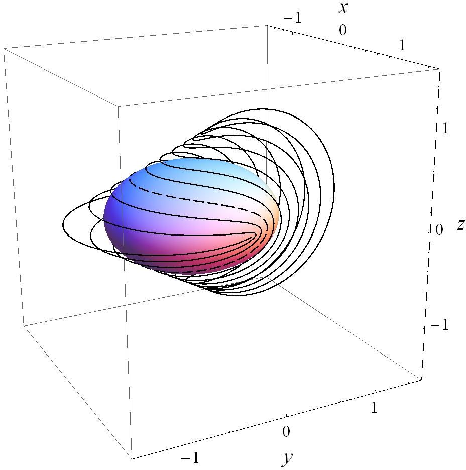
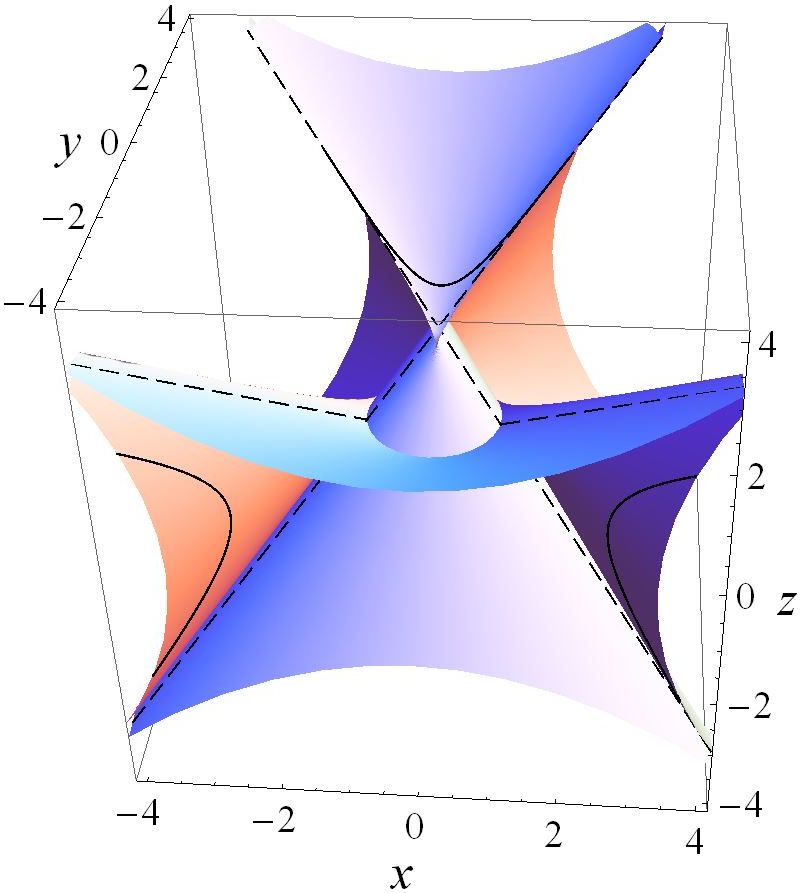
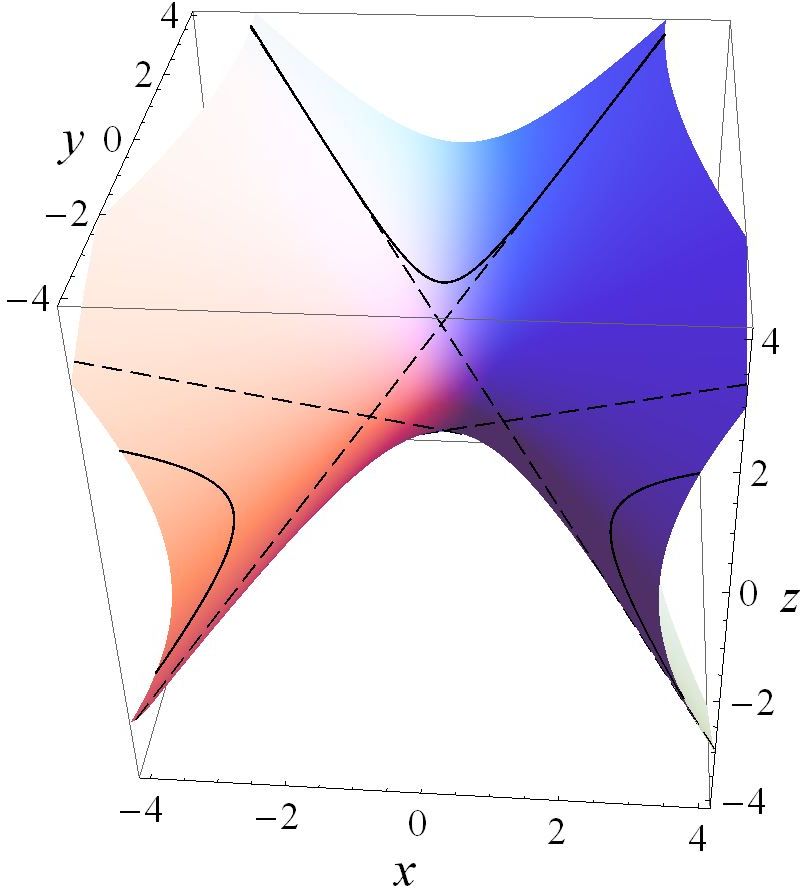
Examples with inscribed quadric and touching curves are shown in Fig. 2 and Fig. 3.

Remark 2.

In the special case λ=1/2𝜆12\lambda=1/2 one gets the equations

x=sint2+cost,y=3cost2(2+cost),z=±1+2cost2+costformulae-sequence𝑥𝑡2𝑡formulae-sequence𝑦3𝑡22𝑡𝑧plus-or-minus12𝑡2𝑡x=\frac{\sin t}{2+\cos t}\,,\quad y=-\frac{3\cos t}{2(2+\cos t)}\,,\quad z=\pm\frac{\sqrt{1+2\cos t}}{2+\cos t}

of the inscribed ellipsoid in [2, p. 115, Eq. (27)].

3 Properties of the touching curves 𝒞λsubscript𝒞𝜆\mathcal{C}_{\lambda}

Since fλ(x,y,z)subscript𝑓𝜆𝑥𝑦𝑧f_{\lambda}(-x,y,z) =fλ(x,y,z)absentsubscript𝑓𝜆𝑥𝑦𝑧=f_{\lambda}(x,y,z) and fλ(x,y,z)=fλ(x,y,z)subscript𝑓𝜆𝑥𝑦𝑧subscript𝑓𝜆𝑥𝑦𝑧f_{\lambda}(x,y,-z)=f_{\lambda}(x,y,z), every quadric 𝒬λsubscript𝒬𝜆\mathcal{Q}_{\lambda} is symmetric with respect to 𝒳𝒳\mathcal{X} and 𝒵𝒵\mathcal{Z}. The extended oloid 𝒪𝒪\mathcal{O} is symmetric with respect to these planes, too. It follows that all touching curves 𝒞λsubscript𝒞𝜆\mathcal{C}_{\lambda} are symmetric with respect to 𝒳𝒳\mathcal{X} and 𝒵𝒵\mathcal{Z}. We denote by X1subscript𝑋1X_{1}, X2subscript𝑋2X_{2} the intersection points of 𝒞λsubscript𝒞𝜆\mathcal{C}_{\lambda} and 𝒳𝒳\mathcal{X}, and by Z1subscript𝑍1Z_{1}, Z2subscript𝑍2Z_{2} those of 𝒞λsubscript𝒞𝜆\mathcal{C}_{\lambda} and 𝒵𝒵\mathcal{Z}, and find

X1=X1(λ)=γ(λ,0)=(0,3(1λ)2(1+λ),3λ1+λ),Z1=Z1(λ)=γ(λ,2π3)=(3(1λ)2λ,3λ2(2λ), 0),X2=X2(λ)=γ(λ,4π3)=(0,3(1λ)2(1+λ),3λ1+λ),Z2=Z2(λ)=γ(λ,2π)=(3(1λ)2λ,3λ2(2λ), 0).}\left.\begin{aligned} X_{1}=X_{1}(\lambda)={}&\gamma(\lambda,0)=\left(0,\,-\frac{3(1-\lambda)}{2(1+\lambda)},\,\frac{\sqrt{3}\,\lambda}{1+\lambda}\right),\\[2.84544pt] Z_{1}=Z_{1}(\lambda)={}&\gamma\left(\lambda,\,\frac{2\pi}{3}\right)=\left(\frac{\sqrt{3}\,(1-\lambda)}{2-\lambda},\,\frac{3\lambda}{2(2-\lambda)},\,0\right),\\[2.84544pt] X_{2}=X_{2}(\lambda)={}&\gamma\left(\lambda,\,\frac{4\pi}{3}\right)=\left(0,\,-\frac{3(1-\lambda)}{2(1+\lambda)},\,-\frac{\sqrt{3}\,\lambda}{1+\lambda}\right),\\[2.84544pt] Z_{2}=Z_{2}(\lambda)={}&\gamma(\lambda,2\pi)=\left(-\frac{\sqrt{3}\,(1-\lambda)}{2-\lambda},\,\frac{3\lambda}{2(2-\lambda)},\,0\right).\end{aligned}\;\;\right\} (4)

One easily finds the parametrization 𝒯λsubscript𝒯𝜆\mathcal{T}_{\lambda} for the tangent of 𝒞λsubscript𝒞𝜆\mathcal{C}_{\lambda} in the point γ(λ,t)𝛾𝜆𝑡\gamma(\lambda,t):

𝒯λ(t)={{(x,y,z)3|x=τ1(λ,t,μ),y=τ2(λ,t,μ),z=τ3(λ,t,μ);μ}iftI1,{(x,y,z)3|x=τ1(λ,4π3t,μ),y=τ2(λ,4π3t,μ),z=τ3(λ,4π3t,μ);μ}iftI2,}\mathcal{T}_{\lambda}(t)=\left\{\!\!\begin{array}[]{ll}\big{\{}(x,y,z)\in\mathbb{R}^{3}\>\big{|}\>x=\tau_{1}(\lambda,t,\mu),\,y=\tau_{2}(\lambda,t,\mu),\\[3.41418pt] \hskip 8.5359ptz=\tau_{3}(\lambda,t,\mu)\,;\,\mu\in\mathbb{R}\big{\}}\hskip 47.51604pt\mbox{if}\quad t\in I_{1}\,,\\[9.95863pt] \left\{(x,y,z)\in\mathbb{R}^{3}\>\big{|}\>x=\tau_{1}\!\left(\lambda,\,\tfrac{4\pi}{3}\!-\!t,\,\mu\right)\!,\,y=\tau_{2}\!\left(\lambda,\,\tfrac{4\pi}{3}\!-\!t,\,\mu\right)\!,\right.\\[3.41418pt] \hskip 8.5359ptz=\left.-\tau_{3}\!\left(\lambda,\,\tfrac{4\pi}{3}\!-\!t,\,\mu\right)\!;\,\mu\in\mathbb{R}\right\}\quad\mbox{if}\quad t\in I_{2}\,,\end{array}\right\} (5)

with

τj(λ,t,μ)=κj(λ,t)+μκ˙j(λ,t),κ˙j=dκj(λ,t)dt,j=1,2,3,formulae-sequencesubscript𝜏𝑗𝜆𝑡𝜇subscript𝜅𝑗𝜆𝑡𝜇subscript˙𝜅𝑗𝜆𝑡formulae-sequencesubscript˙𝜅𝑗dsubscript𝜅𝑗𝜆𝑡d𝑡𝑗123\tau_{j}(\lambda,t,\mu)=\kappa_{j}(\lambda,t)+\mu\,\dot{\kappa}_{j}(\lambda,t)\,,\quad\dot{\kappa}_{j}=\frac{\mathrm{d}\kappa_{j}(\lambda,t)}{\mathrm{d}t}\,,\quad j=1,2,3\,,

where

κ˙1(λ,t)=subscript˙𝜅1𝜆𝑡absent\displaystyle\dot{\kappa}_{1}(\lambda,t)={} (1λ)(λ+cost)(1+λcost)2,κ˙2(λ,t)=(1λ+λ2)sint(1+λcost)2,1𝜆𝜆𝑡superscript1𝜆𝑡2subscript˙𝜅2𝜆𝑡1𝜆superscript𝜆2𝑡superscript1𝜆𝑡2\displaystyle\frac{(1-\lambda)(\lambda+\cos t)}{(1+\lambda\cos t)^{2}}\,,\quad\dot{\kappa}_{2}(\lambda,t)=\frac{(1-\lambda+\lambda^{2})\sin t}{(1+\lambda\cos t)^{2}}\,,
κ˙3(λ,t)=subscript˙𝜅3𝜆𝑡absent\displaystyle\dot{\kappa}_{3}(\lambda,t)={} λ[λ(1+cost)1]sint(1+λcost)21+2cost.𝜆delimited-[]𝜆1𝑡1𝑡superscript1𝜆𝑡212𝑡\displaystyle\frac{\lambda[\lambda(1+\cos t)-1]\sin t}{(1+\lambda\cos t)^{2}\,\sqrt{1+2\cos t}}\,.
Refer to caption
Fig. 2: Touching curves 𝒞λsubscript𝒞𝜆\mathcal{C}_{\lambda}, λ=0, 0.1, 0.2,, 0.9, 1𝜆00.10.20.91\lambda=0,\,0.1,\,0.2,\ldots,\,0.9,\,1, and ellipsoid 𝒬0.3subscript𝒬0.3\mathcal{Q}_{0.3} in the box 1.5x,y,z1.5formulae-sequence1.5𝑥𝑦𝑧1.5-1.5\leq x,y,z\leq 1.5; 𝒞0.3subscript𝒞0.3\mathcal{C}_{0.3} with dashed line
Refer to caption
Refer to caption
Fig. 3: Extended oloid 𝒪𝒪\mathcal{O} (left) and hyperboloid 𝒬4subscript𝒬4\mathcal{Q}_{4} (right) with touching curve  𝒞4subscript𝒞4\mathcal{C}_{4} (solid lines) and common generating lines 𝒢j(4)subscript𝒢𝑗4\mathcal{G}_{j}(4), j=1,2,3,4𝑗1234j=1,2,3,4, (dashed) in the box 4x,y,z4formulae-sequence4𝑥𝑦𝑧4-4\leq x,y,z\leq 4

We consider the function 1+λcost1𝜆𝑡1+\lambda\cos t in the denominator of κ1,κ2,κ3subscript𝜅1subscript𝜅2subscript𝜅3\kappa_{1},\kappa_{2},\kappa_{3}. It vanishes in the interval I1subscript𝐼1I_{1} for t=±arccos(1/λ)𝑡plus-or-minus1𝜆t=\pm\arccos(-1/\lambda) if λ(1,2)𝜆12\lambda\in\mathbb{R}\setminus(-1,2). (For λ=1𝜆1\lambda=-1, we have t=0𝑡0t=0; and for λ=2𝜆2\lambda=2, t=±2π/3𝑡plus-or-minus2𝜋3t=\pm 2\pi/3.) 1+λcost1𝜆𝑡1+\lambda\cos t has no zeros in I1subscript𝐼1I_{1} if λ(1,2)𝜆12\lambda\in(-1,2). Therefore, κ1,κ2,κ3subscript𝜅1subscript𝜅2subscript𝜅3\kappa_{1},\kappa_{2},\kappa_{3} are continuous functions if λ(1,2)𝜆12\lambda\in(-1,2); they are not continous if λ(1,2)𝜆12\lambda\in\mathbb{R}\setminus(-1,2). So we have to distinguish the following cases:
Case 1: 1<λ<21𝜆2-1<\lambda<2 Since κ1,κ2,κ3subscript𝜅1subscript𝜅2subscript𝜅3\kappa_{1},\kappa_{2},\kappa_{3} are continuous functions, and

γ2(λ,2π/3)=Z1(λ)=γ1(λ,2π/3),γ2(λ,2π)=Z2(λ)=γ1(λ,2π/3),formulae-sequencesubscript𝛾2𝜆2𝜋3subscript𝑍1𝜆subscript𝛾1𝜆2𝜋3subscript𝛾2𝜆2𝜋subscript𝑍2𝜆subscript𝛾1𝜆2𝜋3\gamma_{2}(\lambda,2\pi/3)=Z_{1}(\lambda)=\gamma_{1}(\lambda,2\pi/3),\quad\gamma_{2}(\lambda,2\pi)=Z_{2}(\lambda)=\gamma_{1}(\lambda,-2\pi/3),

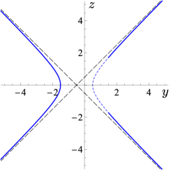
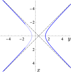
the curve 𝒞λsubscript𝒞𝜆\mathcal{C}_{\lambda} is closed (see Fig. 2). As an example with λ[0,1]𝜆01\lambda\notin[0,1], Fig. 7 shows two projections of 𝒞0.87subscript𝒞0.87\mathcal{C}_{-0.87}. The projection of 𝒞0.87subscript𝒞0.87\mathcal{C}_{-0.87} onto the plane 𝒳𝒳\mathcal{X} (thick line in the diagram on the left of Fig. 7) is part of the left branch of the hyperbola with center point y=29831/499380.597𝑦29831499380.597y=29831/49938\approx 0.597, z=0𝑧0z=0.
Case 2: λ[1,2]𝜆12\lambda\in\mathbb{R}\setminus[-1,2] The parametrization γ(λ,t)𝛾𝜆𝑡\gamma(\lambda,t) of 𝒞λsubscript𝒞𝜆\mathcal{C}_{\lambda} has poles for

t1=subscript𝑡1absent\displaystyle t_{1}={} arccos(1λ),t2=arccos(1λ),1𝜆subscript𝑡21𝜆\displaystyle\!-\!\arccos\left(\!-\frac{1}{\lambda}\right),\hskip 24.18501ptt_{2}=\arccos\left(\!-\frac{1}{\lambda}\right),
t3=subscript𝑡3absent\displaystyle t_{3}={} 4π3arccos(1λ),t4=4π3+arccos(1λ).4𝜋31𝜆subscript𝑡44𝜋31𝜆\displaystyle\frac{4\pi}{3}-\arccos\left(\!-\frac{1}{\lambda}\right),\quad t_{4}=\frac{4\pi}{3}+\arccos\left(\!-\frac{1}{\lambda}\right).

Therefore, it consists of four branches. We calculate the asymptotes of 𝒞λsubscript𝒞𝜆\mathcal{C}_{\lambda} in the poles. For tI1𝑡subscript𝐼1t\in I_{1} the tangent 𝒯λ(t)subscript𝒯𝜆𝑡\mathcal{T}_{\lambda}(t) intersects 𝒳𝒳\mathcal{X} in the point with the coordinates

y=𝑦absent\displaystyle y={} κ2(λ,t)κ˙2(λ,t)κ˙1(λ,t)κ1(λ,t)=λ2+(2λ1)cost2(λ+cost),subscript𝜅2𝜆𝑡subscript˙𝜅2𝜆𝑡subscript˙𝜅1𝜆𝑡subscript𝜅1𝜆𝑡𝜆22𝜆1𝑡2𝜆𝑡\displaystyle\kappa_{2}(\lambda,t)-\frac{\dot{\kappa}_{2}(\lambda,t)}{\dot{\kappa}_{1}(\lambda,t)}\,\kappa_{1}(\lambda,t)=\frac{\lambda-2+(2\lambda-1)\cos t}{2(\lambda+\cos t)}\,,
z=𝑧absent\displaystyle z={} κ3(λ,t)κ˙3(λ,t)κ˙1(λ,t)κ1(λ,t)=λ(1+cost+cos2t)(λ+cost)1+2cost,subscript𝜅3𝜆𝑡subscript˙𝜅3𝜆𝑡subscript˙𝜅1𝜆𝑡subscript𝜅1𝜆𝑡𝜆1𝑡superscript2𝑡𝜆𝑡12𝑡\displaystyle\kappa_{3}(\lambda,t)-\frac{\dot{\kappa}_{3}(\lambda,t)}{\dot{\kappa}_{1}(\lambda,t)}\,\kappa_{1}(\lambda,t)=\frac{\lambda(1+\cos t+\cos^{2}t)}{(\lambda+\cos t)\,\sqrt{1+2\cos t}}\,,

and 𝒵𝒵\mathcal{Z} in

x=𝑥absent\displaystyle x={} κ1(λ,t)κ˙1(λ,t)κ˙3(λ,t)κ3(λ,t)=(λ1)(1+cost+cos2t)[λ(1+cost)1]sint,subscript𝜅1𝜆𝑡subscript˙𝜅1𝜆𝑡subscript˙𝜅3𝜆𝑡subscript𝜅3𝜆𝑡𝜆11𝑡superscript2𝑡delimited-[]𝜆1𝑡1𝑡\displaystyle\kappa_{1}(\lambda,t)-\frac{\dot{\kappa}_{1}(\lambda,t)}{\dot{\kappa}_{3}(\lambda,t)}\,\kappa_{3}(\lambda,t)=\frac{(\lambda-1)(1+\cos t+\cos^{2}t)}{[\lambda(1+\cos t)-1]\sin t}\,,
y=𝑦absent\displaystyle y={} κ2(λ,t)κ˙2(λ,t)κ˙3(λ,t)κ3(λ,t)=1+λ+(2λ)cost2[λ(1+cost)1].subscript𝜅2𝜆𝑡subscript˙𝜅2𝜆𝑡subscript˙𝜅3𝜆𝑡subscript𝜅3𝜆𝑡1𝜆2𝜆𝑡2delimited-[]𝜆1𝑡1\displaystyle\kappa_{2}(\lambda,t)-\frac{\dot{\kappa}_{2}(\lambda,t)}{\dot{\kappa}_{3}(\lambda,t)}\,\kappa_{3}(\lambda,t)=-\frac{1+\lambda+(2-\lambda)\cos t}{2[\lambda(1+\cos t)-1]}\,.

For t=t1𝑡subscript𝑡1t=t_{1} one finds that the asymptote 𝒯λ(t1)subscript𝒯𝜆subscript𝑡1\mathcal{T}_{\lambda}(t_{1}) intersects 𝒵𝒵\mathcal{Z} in the point

(x1,y1,z1)=(1λ+λ22+λλ211λ2,22λλ22λ(λ2), 0),subscript𝑥1subscript𝑦1subscript𝑧11𝜆superscript𝜆22𝜆superscript𝜆211superscript𝜆222𝜆superscript𝜆22𝜆𝜆2 0(x_{1},y_{1},z_{1})=\left(\frac{1-\lambda+\lambda^{2}}{2+\lambda-\lambda^{2}}\,\sqrt{1-\frac{1}{\lambda^{2}}}\,,\;\frac{2-2\lambda-\lambda^{2}}{2\lambda(\lambda-2)}\,,\;0\right),

and 𝒳𝒳\mathcal{X} in

(x~1,y~1,z~1)=(0,14λ+λ22(λ21),1λ+λ2λ21λλ2).subscript~𝑥1subscript~𝑦1subscript~𝑧1014𝜆superscript𝜆22superscript𝜆211𝜆superscript𝜆2superscript𝜆21𝜆𝜆2(\tilde{x}_{1},\tilde{y}_{1},\tilde{z}_{1})=\left(0\,,\;\frac{1-4\lambda+\lambda^{2}}{2(\lambda^{2}-1)}\,,\;\frac{1-\lambda+\lambda^{2}}{\lambda^{2}-1}\,\sqrt{\frac{\lambda}{\lambda-2}}\,\right).

Hence, a parametrization 𝒜1(λ)subscript𝒜1𝜆\mathcal{A}_{1}(\lambda) of the asymptote 𝒯λ(t1)subscript𝒯𝜆subscript𝑡1\mathcal{T}_{\lambda}(t_{1}) is

𝒜1(λ)={(x,y,z)3|x=τ~1(λ,ν),y=τ~2(λ,ν),z=τ~3(λ,ν);ν}subscript𝒜1𝜆conditional-set𝑥𝑦𝑧superscript3formulae-sequence𝑥subscript~𝜏1𝜆𝜈formulae-sequence𝑦subscript~𝜏2𝜆𝜈formulae-sequence𝑧subscript~𝜏3𝜆𝜈𝜈\mathcal{A}_{1}(\lambda)=\{(x,y,z)\in\mathbb{R}^{3}\>\big{|}\>x=\tilde{\tau}_{1}(\lambda,\nu),\,y=\tilde{\tau}_{2}(\lambda,\nu),\,z=\tilde{\tau}_{3}(\lambda,\nu);\,\nu\in\mathbb{R}\}

with

τ~1(λ,ν):=x1+ν(x~1x1)=assignsubscript~𝜏1𝜆𝜈subscript𝑥1𝜈subscript~𝑥1subscript𝑥1absent\displaystyle\tilde{\tau}_{1}(\lambda,\nu):=x_{1}+\nu\,(\tilde{x}_{1}-x_{1})={} 1λ+λ22+λλ211λ2(1ν),1𝜆superscript𝜆22𝜆superscript𝜆211superscript𝜆21𝜈\displaystyle\frac{1-\lambda+\lambda^{2}}{2+\lambda-\lambda^{2}}\,\sqrt{1-\frac{1}{\lambda^{2}}}\;\,(1-\nu)\,,
τ~2(λ,ν):=y1+ν(y~1y1)=assignsubscript~𝜏2𝜆𝜈subscript𝑦1𝜈subscript~𝑦1subscript𝑦1absent\displaystyle\tilde{\tau}_{2}(\lambda,\nu):=\,y_{1}+\nu\,(\tilde{y}_{1}-y_{1})={} 22λλ22λ(λ2)+ν(1λ+λ2)2λ(λ2)(λ21),22𝜆superscript𝜆22𝜆𝜆2𝜈superscript1𝜆superscript𝜆22𝜆𝜆2superscript𝜆21\displaystyle\frac{2-2\lambda-\lambda^{2}}{2\lambda(\lambda-2)}+\nu\,\frac{(1-\lambda+\lambda^{2})^{2}}{\lambda(\lambda-2)(\lambda^{2}-1)}\,,
τ~3(λ,ν):=z1+ν(z~1z1)=assignsubscript~𝜏3𝜆𝜈subscript𝑧1𝜈subscript~𝑧1subscript𝑧1absent\displaystyle\tilde{\tau}_{3}(\lambda,\nu):=\,z_{1}+\nu\,(\tilde{z}_{1}-z_{1})={} ν1λ+λ2λ21λλ2.𝜈1𝜆superscript𝜆2superscript𝜆21𝜆𝜆2\displaystyle\nu\,\frac{1-\lambda+\lambda^{2}}{\lambda^{2}-1}\,\sqrt{\frac{\lambda}{\lambda-2}}\,.

In order to abbreviate notation we write

𝒜1(λ)={(τ~1(λ,ν),τ~2(λ,ν),τ~3(λ,ν))|ν}.subscript𝒜1𝜆conditional-setsubscript~𝜏1𝜆𝜈subscript~𝜏2𝜆𝜈subscript~𝜏3𝜆𝜈𝜈\mathcal{A}_{1}(\lambda)=\{(\tilde{\tau}_{1}(\lambda,\nu),\,\tilde{\tau}_{2}(\lambda,\nu),\,\tilde{\tau}_{3}(\lambda,\nu))\>|\>\nu\in\mathbb{R}\}\,.

The remaining asymptotes are

t=t2:𝒜2(λ)=\displaystyle t=t_{2}\!:\quad\mathcal{A}_{2}(\lambda)={} {(τ~1(λ,ν),τ~2(λ,ν),τ~3(λ,ν))|ν},conditional-setsubscript~𝜏1𝜆𝜈subscript~𝜏2𝜆𝜈subscript~𝜏3𝜆𝜈𝜈\displaystyle\{(-\tilde{\tau}_{1}(\lambda,\nu),\,\tilde{\tau}_{2}(\lambda,\nu),\,\tilde{\tau}_{3}(\lambda,\nu))\>|\>\nu\in\mathbb{R}\}\,,
t=t3:𝒜3(λ)=\displaystyle t=t_{3}\!:\quad\mathcal{A}_{3}(\lambda)={} {(τ~1(λ,ν),τ~2(λ,ν),τ~3(λ,ν))|ν},conditional-setsubscript~𝜏1𝜆𝜈subscript~𝜏2𝜆𝜈subscript~𝜏3𝜆𝜈𝜈\displaystyle\{(-\tilde{\tau}_{1}(\lambda,\nu),\,\tilde{\tau}_{2}(\lambda,\nu),\,-\tilde{\tau}_{3}(\lambda,\nu))\>|\>\nu\in\mathbb{R}\}\,,
t=t4:𝒜4(λ)=\displaystyle t=t_{4}\!:\quad\mathcal{A}_{4}(\lambda)={} {(τ~1(λ,ν),τ~2(λ,ν),τ~3(λ,ν))|ν}.conditional-setsubscript~𝜏1𝜆𝜈subscript~𝜏2𝜆𝜈subscript~𝜏3𝜆𝜈𝜈\displaystyle\{(\tilde{\tau}_{1}(\lambda,\nu),\,\tilde{\tau}_{2}(\lambda,\nu),\,-\tilde{\tau}_{3}(\lambda,\nu))\>|\>\nu\in\mathbb{R}\}\,.

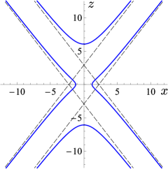
As an example, Fig. 5 shows two projections of the touching curve 𝒞1.4subscript𝒞1.4\mathcal{C}_{-1.4}. The projection onto the plane 𝒳𝒳\mathcal{X} (thick line) is part of a hyperbola with center point y=71/2380.298𝑦712380.298y=71/238\approx 0.298, z=0𝑧0z=0.
Case 3: λ=±𝜆plus-or-minus\lambda=\pm\infty For γ(t):=limλ±γ(λ,t)assignsuperscript𝛾𝑡subscript𝜆plus-or-minus𝛾𝜆𝑡\gamma^{*}(t):=\lim_{\lambda\rightarrow\pm\infty}\gamma(\lambda,t) one easily finds

γ:I1I23,tγ(t)={γ1(t)iftI1,γ2(t)iftI2,:superscript𝛾formulae-sequencesubscript𝐼1subscript𝐼2superscript3maps-to𝑡superscript𝛾𝑡casessuperscriptsubscript𝛾1𝑡if𝑡subscript𝐼1superscriptsubscript𝛾2𝑡if𝑡subscript𝐼2\displaystyle\gamma^{*}:\;I_{1}\cup I_{2}\rightarrow\mathbb{R}^{3}\,,\quad t\;\mapsto\gamma^{*}(t)=\left\{\begin{array}[]{l@{\quad\mbox{if}\quad}l}\gamma_{1}^{*}(t)&t\in I_{1}\,,\\[5.69046pt] \gamma_{2}^{*}(t)&t\in I_{2}\,,\end{array}\right.

with

γ1(t)=superscriptsubscript𝛾1𝑡absent\displaystyle\gamma_{1}^{*}(t)={} (κ1(t),κ2(t),κ3(t)),superscriptsubscript𝜅1𝑡superscriptsubscript𝜅2𝑡superscriptsubscript𝜅3𝑡\displaystyle\big{(}\kappa_{1}^{*}(t),\,\kappa_{2}^{*}(t),\,\kappa_{3}^{*}(t)\big{)},
γ2(t)=superscriptsubscript𝛾2𝑡absent\displaystyle\gamma_{2}^{*}(t)={} (κ1(4π3t),κ2(4π3t),κ3(4π3t)),superscriptsubscript𝜅14𝜋3𝑡superscriptsubscript𝜅24𝜋3𝑡superscriptsubscript𝜅34𝜋3𝑡\displaystyle\!\left(\kappa_{1}^{*}\!\left(\frac{4\pi}{3}-t\right)\!,\;\kappa_{2}^{*}\!\left(\frac{4\pi}{3}-t\right)\!,\;-\kappa_{3}^{*}\!\left(\frac{4\pi}{3}-t\right)\!\right),

where

κ1(t)=superscriptsubscript𝜅1𝑡absent\displaystyle\kappa_{1}^{*}(t)={} limλ±κ1(λ,t)=tant,subscript𝜆plus-or-minussubscript𝜅1𝜆𝑡𝑡\displaystyle\lim_{\lambda\rightarrow\pm\infty}\kappa_{1}(\lambda,t)=-\tan t\,,
κ2(t)=superscriptsubscript𝜅2𝑡absent\displaystyle\kappa_{2}^{*}(t)={} limλ±κ2(λ,t)=12+1cost,subscript𝜆plus-or-minussubscript𝜅2𝜆𝑡121𝑡\displaystyle\lim_{\lambda\rightarrow\pm\infty}\kappa_{2}(\lambda,t)=\frac{1}{2}+\frac{1}{\cos t}\,,
κ3(t)=superscriptsubscript𝜅3𝑡absent\displaystyle\kappa_{3}^{*}(t)={} limλ±κ3(λ,t)=1+2costcost.subscript𝜆plus-or-minussubscript𝜅3𝜆𝑡12𝑡𝑡\displaystyle\lim_{\lambda\rightarrow\pm\infty}\kappa_{3}(\lambda,t)=\frac{\sqrt{1+2\cos t}}{\cos t}\,.

The parametrization γ(t)superscript𝛾𝑡\gamma^{*}(t) of 𝒞±subscript𝒞plus-or-minus\mathcal{C}_{\pm\infty} has poles for

t1=π2,t2=π2,t3=4π3π2=5π6,t4=4π3+π2=11π6,formulae-sequenceformulae-sequencesubscript𝑡1𝜋2formulae-sequencesubscript𝑡2𝜋2subscript𝑡34𝜋3𝜋25𝜋6subscript𝑡44𝜋3𝜋211𝜋6t_{1}=-\frac{\pi}{2}\,,\quad t_{2}=\frac{\pi}{2}\,,\quad t_{3}=\frac{4\pi}{3}-\frac{\pi}{2}=\frac{5\pi}{6}\,,\quad t_{4}=\frac{4\pi}{3}+\frac{\pi}{2}=\frac{11\pi}{6}\,,

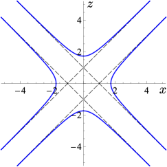
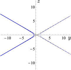
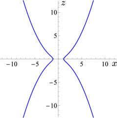
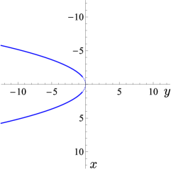
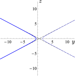
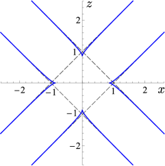
and therefore, 𝒞±subscript𝒞plus-or-minus\mathcal{C}_{\pm\infty} consists of four branches (see Fig. 4). For the asymptotes of 𝒞±subscript𝒞plus-or-minus\mathcal{C}_{\pm\infty} we find

limλ±𝒜1(λ)={(ν1,ν1/2,ν)|ν},limλ±𝒜2(λ)={(1ν,ν1/2,ν)|ν},limλ±𝒜3(λ)={(1ν,ν1/2,ν)|ν},limλ±𝒜4(λ)={(ν1,ν1/2,ν)|ν},}\left.\begin{aligned} \lim_{\lambda\rightarrow\pm\infty}\mathcal{A}_{1}(\lambda)={}&\left\{\left(\nu-1,\,\nu-1/2,\,\nu\right)\>|\>\nu\in\mathbb{R}\right\},\\[2.84544pt] \lim_{\lambda\rightarrow\pm\infty}\mathcal{A}_{2}(\lambda)={}&\left\{\left(1-\nu,\,\nu-1/2,\,\nu\right)\>|\>\nu\in\mathbb{R}\right\},\\[2.84544pt] \lim_{\lambda\rightarrow\pm\infty}\mathcal{A}_{3}(\lambda)={}&\left\{\left(1-\nu,\,\nu-1/2,\,-\nu\right)\>|\>\nu\in\mathbb{R}\right\},\\[2.84544pt] \lim_{\lambda\rightarrow\pm\infty}\mathcal{A}_{4}(\lambda)={}&\left\{\left(\nu-1,\,\nu-1/2,\,-\nu\right)\>|\>\nu\in\mathbb{R}\right\},\end{aligned}\;\;\right\} (6)

and from (4) for the intersection points,

limλ±X1(λ)=subscript𝜆plus-or-minussubscript𝑋1𝜆absent\displaystyle\lim_{\lambda\rightarrow\pm\infty}X_{1}(\lambda)={} (0,32,3),limλ±Z1(λ)=(3,32, 0),0323subscript𝜆plus-or-minussubscript𝑍1𝜆332 0\displaystyle\left(0\,,\>\frac{3}{2}\,,\>\sqrt{3}\right),\hskip 18.49411pt\lim_{\lambda\rightarrow\pm\infty}Z_{1}(\lambda)=\left(\sqrt{3}\,,\>-\frac{3}{2}\,,\>0\right),
limλ±X2(λ)=subscript𝜆plus-or-minussubscript𝑋2𝜆absent\displaystyle\lim_{\lambda\rightarrow\pm\infty}X_{2}(\lambda)={} (0,32,3),limλ±Z2(λ)=(3,32, 0).0323subscript𝜆plus-or-minussubscript𝑍2𝜆332 0\displaystyle\left(0\,,\>\frac{3}{2}\,,\>-\sqrt{3}\right),\quad\lim_{\lambda\rightarrow\pm\infty}Z_{2}(\lambda)=\left(-\sqrt{3}\,,\>-\frac{3}{2}\,,\>0\right).

From the parametrization γ(t)superscript𝛾𝑡\gamma^{*}(t) of 𝒞±subscript𝒞plus-or-minus\mathcal{C}_{\pm\infty} we have

x2=tan2t=1cos2tcos2t,y=12+1cost,z2=1+2costcos2t.formulae-sequencesuperscript𝑥2superscript2𝑡1superscript2𝑡superscript2𝑡formulae-sequence𝑦121𝑡superscript𝑧212𝑡superscript2𝑡x^{2}=\tan^{2}t=\frac{1-\cos^{2}t}{\cos^{2}t}\,,\quad y=\frac{1}{2}+\frac{1}{\cos t}\,,\quad z^{2}=\frac{1+2\cos t}{\cos^{2}t}\,.

By eliminating cost𝑡\cos t we find the following algebraic equations of the projections of 𝒞±subscript𝒞plus-or-minus\mathcal{C}_{\pm\infty} onto the planes 𝒳𝒳\mathcal{X}, 𝒴𝒴\mathcal{Y}, 𝒵𝒵\mathcal{Z}:

projection onto 𝒳𝒳\mathcal{X}: (y+12)2z2=1,superscript𝑦122superscript𝑧21\displaystyle\left(y+\tfrac{1}{2}\right)^{2}-z^{2}=1\,, (7)
𝒴𝒴\mathcal{Y}: (x2z2)22(x2+z2)=3,superscriptsuperscript𝑥2superscript𝑧222superscript𝑥2superscript𝑧23\displaystyle\left(x^{2}-z^{2}\right)^{2}-2\left(x^{2}+z^{2}\right)=3\,, (8)
𝒵𝒵\mathcal{Z}: (y12)2x2=1.superscript𝑦122superscript𝑥21\displaystyle\left(y-\tfrac{1}{2}\right)^{2}-x^{2}=1\,. (9)

Formulas (7) and (9)italic-(9italic-)\eqref{Z-hyperbola} are the equations of hyperbolas with center points y=1/2𝑦12y=-1/2, z=0𝑧0z=0, and x=0𝑥0x=0, y=1/2𝑦12y=1/2, respectively. The actual projections of 𝒞±subscript𝒞plus-or-minus\mathcal{C}_{\pm\infty} onto 𝒳𝒳\mathcal{X} and 𝒵𝒵\mathcal{Z} (plotted with thick lines) are part of the respective hyperbola.
Case 4: λ{1,2}𝜆12\lambda\in\{-1,2\} 𝒞λsubscript𝒞𝜆\mathcal{C}_{\lambda} consists of two branches. For λ=1𝜆1\lambda=-1, from (4) it follows that

limε0X1(1ε)=(0,,),limε0X1(1+ε)=(0,,),formulae-sequencesubscript𝜀0subscript𝑋11𝜀0subscript𝜀0subscript𝑋11𝜀0\displaystyle\lim_{\varepsilon\rightarrow 0}X_{1}(-1-\varepsilon)=(0,\infty,\infty)\,,\hskip 19.91684pt\lim_{\varepsilon\rightarrow 0}X_{1}(-1+\varepsilon)=(0,-\infty,-\infty)\,,
limε0X2(1ε)=(0,,),limε0X2(1+ε)=(0,,),formulae-sequencesubscript𝜀0subscript𝑋21𝜀0subscript𝜀0subscript𝑋21𝜀0\displaystyle\lim_{\varepsilon\rightarrow 0}X_{2}(-1-\varepsilon)=(0,\infty,-\infty)\,,\quad\lim_{\varepsilon\rightarrow 0}X_{2}(-1+\varepsilon)=(0,-\infty,\infty)\,,
Z1(1)=(23,12, 0),Z2(1)=(23,12, 0),formulae-sequencesubscript𝑍112312 0subscript𝑍212312 0\displaystyle Z_{1}(-1)=\left(\frac{2}{\sqrt{3}}\,,\>-\frac{1}{2}\,,\>0\right),\hskip 31.2982ptZ_{2}(-1)=\left(\!-\frac{2}{\sqrt{3}}\,,\>-\frac{1}{2}\,,\>0\right),
Refer to caption
Refer to caption
Refer to caption
Fig. 4: Projections of 𝒞±subscript𝒞plus-or-minus\mathcal{C}_{\pm\infty} and its asymptotes 𝒜k(±)subscript𝒜𝑘plus-or-minus\mathcal{A}_{k}(\pm\infty), k=1,2,3,4𝑘1234k=1,2,3,4,    onto the planes 𝒳𝒳\mathcal{X}, 𝒴𝒴\mathcal{Y}, and 𝒵𝒵\mathcal{Z};

5x,y,z5formulae-sequence5𝑥𝑦𝑧5-5\leq x,y,z\leq 5

Refer to caption
Refer to caption
Fig. 5: Projections of 𝒞1.4subscript𝒞1.4\mathcal{C}_{-1.4} and its asymptotes 𝒜k(4)subscript𝒜𝑘4\mathcal{A}_{k}(4), k=1,2,3,4𝑘1234k=1,2,3,4, onto the planes 𝒳𝒳\mathcal{X} and 𝒴𝒴\mathcal{Y}; 12x,y,z12formulae-sequence12𝑥𝑦𝑧12-12\leq x,y,z\leq 12
Refer to caption
Refer to caption
Refer to caption
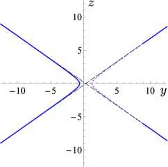
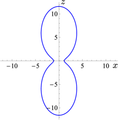
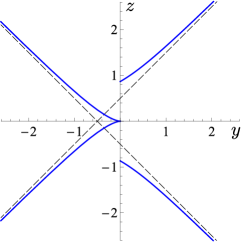
Fig. 6: Projections of 𝒞1subscript𝒞1\mathcal{C}_{-1} onto the planes 𝒳𝒳\mathcal{X}, 𝒴𝒴\mathcal{Y}, and 𝒵𝒵\mathcal{Z};

12x,y,z12formulae-sequence12𝑥𝑦𝑧12-12\leq x,y,z\leq 12

Refer to caption
Refer to caption
Fig. 7: Projections of 𝒞0.87subscript𝒞0.87\mathcal{C}_{-0.87} onto the planes 𝒳𝒳\mathcal{X} and 𝒴𝒴\mathcal{Y}; 12x,y,z12formulae-sequence12𝑥𝑦𝑧12-12\leq x,y,z\leq 12


and for λ=2𝜆2\lambda=2,

X1(2)=(0,12,23),X2(2)=(0,12,23),formulae-sequencesubscript𝑋1201223subscript𝑋2201223\displaystyle X_{1}(2)=\left(0\,,\>\frac{1}{2}\,,\>\frac{2}{\sqrt{3}}\right),\hskip 36.98866ptX_{2}(2)=\left(0\,,\>\frac{1}{2}\,,\>-\frac{2}{\sqrt{3}}\right),
limε0Z1(2ε)=(,,0),limε0Z1(2+ε)=(,,0),formulae-sequencesubscript𝜀0subscript𝑍12𝜀0subscript𝜀0subscript𝑍12𝜀0\displaystyle\lim_{\varepsilon\rightarrow 0}Z_{1}(2-\varepsilon)=(-\infty,\infty,0)\,,\quad\lim_{\varepsilon\rightarrow 0}Z_{1}(2+\varepsilon)=(\infty,-\infty,0)\,,
limε0Z2(2ε)=(,,0),limε0Z2(2+ε)=(,,0).formulae-sequencesubscript𝜀0subscript𝑍22𝜀0subscript𝜀0subscript𝑍22𝜀0\displaystyle\lim_{\varepsilon\rightarrow 0}Z_{2}(2-\varepsilon)=(\infty,\infty,0)\,,\hskip 19.0633pt\lim_{\varepsilon\rightarrow 0}Z_{2}(2+\varepsilon)=(-\infty,-\infty,0)\,.

Projections of 𝒞1subscript𝒞1\mathcal{C}_{-1} are shown in Fig. 6. The projection onto the plane 𝒳𝒳\mathcal{X} is the left branch (thick line) of the hyperbola with the algebraic equation

(y12)23z2=1.superscript𝑦1223superscript𝑧21\left(y-\frac{1}{2}\right)^{2}-3z^{2}=1\,.

The equations of its asymptotes are z=±(y1/2)/3𝑧plus-or-minus𝑦123z=\pm(y-1/2)/\sqrt{3}. The projection of 𝒞1subscript𝒞1\mathcal{C}_{-1} onto 𝒴𝒴\mathcal{Y} has the algebraic equation

3x4+8x264z2=16.3superscript𝑥48superscript𝑥264superscript𝑧2163x^{4}+8x^{2}-64z^{2}=16\,.

The projection onto 𝒵𝒵\mathcal{Z} is part of the parabola with equation x=3y2/8𝑥3superscript𝑦28x=-3y^{2}/8.

4 The edge of regression

In the following we denote by \mathcal{R} the edge of regression of the developable surface 𝒪𝒪\mathcal{O} (see [7, pp. 119-125], and Fig. 1, Fig. 8).

Theorem 2.

For tI1𝑡subscript𝐼1t\in I_{1}, parametric equations of \mathcal{R} are given by

x=g1(t)=𝑥subscript𝑔1𝑡absent\displaystyle x=g_{1}(t)={} sinttant3,y=g2(t)=2+3cost3cos2t2cos3t6(1+cost)cost,𝑡𝑡3𝑦subscript𝑔2𝑡23𝑡3superscript2𝑡2superscript3𝑡61𝑡𝑡\displaystyle\frac{\sin t-\tan t}{3}\,,\quad y=g_{2}(t)=\frac{2+3\cos t-3\cos^{2}t-2\cos^{3}t}{6(1+\cos t)\cos t}\,,
z=g3(t)=𝑧subscript𝑔3𝑡absent\displaystyle z=g_{3}(t)={} ±(1+2cost)3/23(1+cost)cost.plus-or-minussuperscript12𝑡3231𝑡𝑡\displaystyle\!\pm\!\frac{(1+2\cos t)^{3/2}}{3(1+\cos t)\cos t}\,.
Proof.

\mathcal{R} is the solution of the system of equations

fλ(x,y,z)=0,fλ(x,y,z):=λfλ(x,y,z)=0,fλ′′(x,y,z):=2λ2fλ(x,y,z)=0}casesformulae-sequencesubscript𝑓𝜆𝑥𝑦𝑧0assignsubscriptsuperscript𝑓𝜆𝑥𝑦𝑧𝜆subscript𝑓𝜆𝑥𝑦𝑧0assignsubscriptsuperscript𝑓′′𝜆𝑥𝑦𝑧superscript2superscript𝜆2subscript𝑓𝜆𝑥𝑦𝑧0\left.\begin{array}[]{l}f_{\lambda}(x,y,z)\;=0\,,\quad f^{\prime}_{\lambda}(x,y,z):=\dfrac{\partial}{\partial\lambda}\,f_{\lambda}(x,y,z)=0\,,\\[8.5359pt] f^{\prime\prime}_{\lambda}(x,y,z):=\dfrac{\partial^{2}}{\partial\lambda^{2}}\,f_{\lambda}(x,y,z)=0\end{array}\right\}

with variable λ𝜆\lambda, see [1, pp. 523-524]. Since the touching curve 𝒞λsubscript𝒞𝜆\mathcal{C}_{\lambda} is the intersection curve of the quadric 𝒬λsubscript𝒬𝜆\mathcal{Q}_{\lambda} and the quadric defined by fλ(x,y,z)=0subscriptsuperscript𝑓𝜆𝑥𝑦𝑧0f^{\prime}_{\lambda}(x,y,z)=0, the parametric functions κ1subscript𝜅1\kappa_{1}, κ2subscript𝜅2\kappa_{2}, κ3subscript𝜅3\kappa_{3} of 𝒞λsubscript𝒞𝜆\mathcal{C}_{\lambda} are not only solutions of

fλ(κ1(λ,t),κ2(λ,t),κ3(λ,t))=0subscript𝑓𝜆subscript𝜅1𝜆𝑡subscript𝜅2𝜆𝑡subscript𝜅3𝜆𝑡0f_{\lambda}(\kappa_{1}(\lambda,t),\kappa_{2}(\lambda,t),\kappa_{3}(\lambda,t))=0\;\;

but also of

fλ(κ1(λ,t),κ2(λ,t),κ3(λ,t))=0.subscriptsuperscript𝑓𝜆subscript𝜅1𝜆𝑡subscript𝜅2𝜆𝑡subscript𝜅3𝜆𝑡0f^{\prime}_{\lambda}(\kappa_{1}(\lambda,t),\kappa_{2}(\lambda,t),\kappa_{3}(\lambda,t))=0\,.

Furthermore, one finds

fλ′′(x,y,z)subscriptsuperscript𝑓′′𝜆𝑥𝑦𝑧\displaystyle f^{\prime\prime}_{\lambda}(x,y,z)
=\displaystyle={} x2(1λ)3+3y2(λ1)λy(23λ3λ2+2λ3)(1λ+λ2)3+z2λ39(λ1)λ(1λ+λ2)3.superscript𝑥2superscript1𝜆33superscript𝑦2𝜆1𝜆𝑦23𝜆3superscript𝜆22superscript𝜆3superscript1𝜆superscript𝜆23superscript𝑧2superscript𝜆39𝜆1𝜆superscript1𝜆superscript𝜆23\displaystyle\frac{x^{2}}{(1-\lambda)^{3}}+\frac{3y^{2}(\lambda-1)\lambda-y\left(2-3\lambda-3\lambda^{2}+2\lambda^{3}\right)}{\left(1-\lambda+\lambda^{2}\right)^{3}}+\frac{z^{2}}{\lambda^{3}}-\frac{9(\lambda-1)\lambda}{\left(1-\lambda+\lambda^{2}\right)^{3}}\,.

Solving the equation

fλ′′(κ1(λ,t),κ2(λ,t),κ3(λ,t))=0subscriptsuperscript𝑓′′𝜆subscript𝜅1𝜆𝑡subscript𝜅2𝜆𝑡subscript𝜅3𝜆𝑡0f^{\prime\prime}_{\lambda}(\kappa_{1}(\lambda,t),\kappa_{2}(\lambda,t),\kappa_{3}(\lambda,t))=0

for λ𝜆\lambda yields

λ=ϕ(t):=1+2cost(2+cost)cost.𝜆italic-ϕ𝑡assign12𝑡2𝑡𝑡\lambda=\phi(t):=\frac{1+2\cos t}{(2+\cos t)\cos t}\,.

It follows that gj(t):=κj(ϕ(t),t)assignsubscript𝑔𝑗𝑡subscript𝜅𝑗italic-ϕ𝑡𝑡g_{j}(t):=\kappa_{j}(\phi(t),t), j=1,2,3𝑗123j=1,2,3, and

x=g1(t),y=g2(t),z=g3(t).formulae-sequence𝑥subscript𝑔1𝑡formulae-sequence𝑦subscript𝑔2𝑡𝑧subscript𝑔3𝑡x=g_{1}(t)\,,\quad y=g_{2}(t)\,,\quad z=g_{3}(t)\,.

Due to the symmetry of 𝒪𝒪\mathcal{O} with respect to the plane 𝒵𝒵\mathcal{Z}, we also have

x=g1(t),y=g2(t),z=g3(t).formulae-sequence𝑥subscript𝑔1𝑡formulae-sequence𝑦subscript𝑔2𝑡𝑧subscript𝑔3𝑡x=g_{1}(t)\,,\quad y=g_{2}(t)\,,\quad z=-g_{3}(t)\,.\qed
Corollary 2.

With the system parameter λ𝜆\lambda, the edge of regression is given by

=absent\displaystyle\mathcal{R}={} {r1(λ),r2(λ),r3(λ)|λ[0,1]}conditional-setsubscript𝑟1𝜆subscript𝑟2𝜆subscript𝑟3𝜆𝜆01\displaystyle\{r_{1}(\lambda),r_{2}(\lambda),r_{3}(\lambda)\>|\>\lambda\in\mathbb{R}\setminus[0,1]\}
\displaystyle\cup\hskip 3.41418pt{} {r1(λ),r2(λ),r3(λ)|λ[0,1]}conditional-setsubscript𝑟1𝜆subscript𝑟2𝜆subscript𝑟3𝜆𝜆01\displaystyle\{-r_{1}(\lambda),r_{2}(\lambda),r_{3}(\lambda)\>|\>\lambda\in\mathbb{R}\setminus[0,1]\}
\displaystyle\cup\hskip 3.41418pt{} {r1(λ),r2(λ),r3(λ)|λ[0,1]}conditional-setsubscript𝑟1𝜆subscript𝑟2𝜆subscript𝑟3𝜆𝜆01\displaystyle\{-r_{1}(\lambda),r_{2}(\lambda),-r_{3}(\lambda)\>|\>\lambda\in\mathbb{R}\setminus[0,1]\}
\displaystyle\cup\hskip 3.41418pt{} {r1(λ),r2(λ),r3(λ)|λ[0,1]},conditional-setsubscript𝑟1𝜆subscript𝑟2𝜆subscript𝑟3𝜆𝜆01\displaystyle\{r_{1}(\lambda),r_{2}(\lambda),-r_{3}(\lambda)\>|\>\lambda\in\mathbb{R}\setminus[0,1]\}\,,

where

r1(λ)=subscript𝑟1𝜆absent\displaystyle r_{1}(\lambda)={} (λ1)3[2λ+2ρ(λ)]λ[2λ+ρ(λ)],r2(λ)=λ2+2λ2+(λ2)ρ(λ)2λ[2λ+ρ(λ)],superscript𝜆13delimited-[]2𝜆2𝜌𝜆𝜆delimited-[]2𝜆𝜌𝜆subscript𝑟2𝜆superscript𝜆22𝜆2𝜆2𝜌𝜆2𝜆delimited-[]2𝜆𝜌𝜆\displaystyle\frac{\sqrt{(\lambda-1)^{3}\,[2-\lambda+2\rho(\lambda)]}}{\lambda\,[2-\lambda+\rho(\lambda)]}\,,\;\;r_{2}(\lambda)=\frac{\lambda^{2}+2\lambda-2+(\lambda-2)\,\rho(\lambda)}{2\lambda\,[2-\lambda+\rho(\lambda)]}\,,
r3(λ)=subscript𝑟3𝜆absent\displaystyle r_{3}(\lambda)={} sgn(λ)λ[2λ+2ρ(λ)]2λ+ρ(λ),ρ(λ)=sgn(λ)1λ+λ2.sgn𝜆𝜆delimited-[]2𝜆2𝜌𝜆2𝜆𝜌𝜆𝜌𝜆sgn𝜆1𝜆superscript𝜆2\displaystyle\frac{\mathrm{sgn}(\lambda)\,\sqrt{\lambda\,[2-\lambda+2\rho(\lambda)]}}{2-\lambda+\rho(\lambda)}\,,\;\;\;\rho(\lambda)=\mathrm{sgn}(\lambda)\,\sqrt{1-\lambda+\lambda^{2}}\,.
Proof.

We consider the function

ϕ:I1,tϕ(t)=1+2cost(2+cost)cost,:italic-ϕformulae-sequencesubscript𝐼1maps-to𝑡italic-ϕ𝑡12𝑡2𝑡𝑡\phi:\;I_{1}\;\rightarrow\;\mathbb{R}\,,\quad t\;\mapsto\;\phi(t)=\frac{1+2\cos t}{(2+\cos t)\cos t}\,,

used in the proof of Theorem 2. We denote by ϕ1subscriptitalic-ϕ1\phi_{1} the restriction of ϕitalic-ϕ\phi to the interval (2π/3,0)2𝜋30(-2\pi/3,0), and by ϕ2subscriptitalic-ϕ2\phi_{2} the restriction of ϕitalic-ϕ\phi to (0,2π/3)02𝜋3(0,2\pi/3). One easily finds the respective inverse functions

ϕ11(λ)=arccos1λ+ρ(λ)λ,ϕ21(λ)=arccos1λ+ρ(λ)λformulae-sequencesuperscriptsubscriptitalic-ϕ11𝜆1𝜆𝜌𝜆𝜆superscriptsubscriptitalic-ϕ21𝜆1𝜆𝜌𝜆𝜆\phi_{1}^{-1}(\lambda)=-\!\arccos\dfrac{1-\lambda+\rho(\lambda)}{\lambda}\,,\quad\phi_{2}^{-1}(\lambda)=\arccos\dfrac{1-\lambda+\rho(\lambda)}{\lambda}

with ρ(λ):=sgn(λ)1λ+λ2assign𝜌𝜆sgn𝜆1𝜆superscript𝜆2\rho(\lambda):=\mathrm{sgn}(\lambda)\,\sqrt{1-\lambda+\lambda^{2}} and λ[0,1]𝜆01\lambda\in\mathbb{R}\setminus[0,1], hence

r1(λ):=assignsubscript𝑟1𝜆absent\displaystyle r_{1}(\lambda):={} κ1(λ,ϕ11(λ))=(λ1)3[2λ+2ρ(λ)]λ[2λ+ρ(λ)],subscript𝜅1𝜆superscriptsubscriptitalic-ϕ11𝜆superscript𝜆13delimited-[]2𝜆2𝜌𝜆𝜆delimited-[]2𝜆𝜌𝜆\displaystyle\kappa_{1}\big{(}\lambda,\phi_{1}^{-1}(\lambda)\big{)}=\frac{\sqrt{(\lambda-1)^{3}\,[2-\lambda+2\rho(\lambda)]}}{\lambda\,[2-\lambda+\rho(\lambda)]}\,,
r2(λ):=assignsubscript𝑟2𝜆absent\displaystyle r_{2}(\lambda):={} κ2(λ,ϕ11(λ))=λ2+2λ2+(λ2)ρ(λ)2λ[2λ+ρ(λ)],subscript𝜅2𝜆superscriptsubscriptitalic-ϕ11𝜆superscript𝜆22𝜆2𝜆2𝜌𝜆2𝜆delimited-[]2𝜆𝜌𝜆\displaystyle\kappa_{2}\big{(}\lambda,\phi_{1}^{-1}(\lambda)\big{)}=\frac{\lambda^{2}+2\lambda-2+(\lambda-2)\,\rho(\lambda)}{2\lambda\,[2-\lambda+\rho(\lambda)]}\,,
r3(λ):=assignsubscript𝑟3𝜆absent\displaystyle r_{3}(\lambda):={} κ3(λ,ϕ11(λ))=sgn(λ)λ[2λ+2ρ(λ)]2λ+ρ(λ),subscript𝜅3𝜆superscriptsubscriptitalic-ϕ11𝜆sgn𝜆𝜆delimited-[]2𝜆2𝜌𝜆2𝜆𝜌𝜆\displaystyle\kappa_{3}\big{(}\lambda,\phi_{1}^{-1}(\lambda)\big{)}=\frac{\mathrm{sgn}(\lambda)\,\sqrt{\lambda\,[2-\lambda+2\rho(\lambda)]}}{2-\lambda+\rho(\lambda)}\,,

and

κ1(λ,ϕ21(λ))=r1(λ),κ2(λ,ϕ21(λ))=r2(λ),κ3(λ,ϕ21(λ))=r3(λ).formulae-sequencesubscript𝜅1𝜆superscriptsubscriptitalic-ϕ21𝜆subscript𝑟1𝜆formulae-sequencesubscript𝜅2𝜆superscriptsubscriptitalic-ϕ21𝜆subscript𝑟2𝜆subscript𝜅3𝜆superscriptsubscriptitalic-ϕ21𝜆subscript𝑟3𝜆\kappa_{1}\big{(}\lambda,\phi_{2}^{-1}(\lambda)\big{)}=-r_{1}(\lambda)\,,\;\;\kappa_{2}\big{(}\lambda,\phi_{2}^{-1}(\lambda)\big{)}=r_{2}(\lambda)\,,\;\;\kappa_{3}\big{(}\lambda,\phi_{2}^{-1}(\lambda)\big{)}=r_{3}(\lambda)\,.

It follows that

x=±r1(λ),y=r2(λ),z=r3(λ),formulae-sequence𝑥plus-or-minussubscript𝑟1𝜆formulae-sequence𝑦subscript𝑟2𝜆𝑧subscript𝑟3𝜆x=\pm r_{1}(\lambda)\,,\quad y=r_{2}(\lambda)\,,\quad z=r_{3}(\lambda)\,,

and, due to the symmetry of 𝒪𝒪\mathcal{O} with respect to the plane 𝒵𝒵\mathcal{Z}, also

x=±r1(λ),y=r2(λ),z=r3(λ).formulae-sequence𝑥plus-or-minussubscript𝑟1𝜆formulae-sequence𝑦subscript𝑟2𝜆𝑧subscript𝑟3𝜆x=\pm r_{1}(\lambda)\,,\quad y=r_{2}(\lambda)\,,\quad z=-r_{3}(\lambda)\,.\qed

Every generating line of a developable surface is a tangent to its edge of regression. Obviously, t=π/2𝑡𝜋2t=-\pi/2 and t=π/2𝑡𝜋2t=\pi/2 are poles of the functions g1subscript𝑔1g_{1}, g2subscript𝑔2g_{2}, g3subscript𝑔3g_{3} in Theorem 2. One easily finds

ω1(m,π2)=m1,ω2(m,π2)=m12,ω3(m,π2)=m,ω1(m,π2)=1m,ω2(m,π2)=m12,ω3(m,π2)=m.subscript𝜔1𝑚𝜋2absent𝑚1subscript𝜔2𝑚𝜋2absent𝑚12subscript𝜔3𝑚𝜋2absent𝑚subscript𝜔1𝑚𝜋2absent1𝑚subscript𝜔2𝑚𝜋2absent𝑚12subscript𝜔3𝑚𝜋2absent𝑚\begin{array}[]{*2{l@{\;=\;}r@{\,,\quad}}l@{\;=\;}r}\omega_{1}\!\left(m,-\dfrac{\pi}{2}\right)&m-1&\omega_{2}\!\left(m,-\dfrac{\pi}{2}\right)&m-\dfrac{1}{2}&\omega_{3}\!\left(m,-\dfrac{\pi}{2}\right)&m\,,\\[8.5359pt] \omega_{1}\!\left(m,\,\dfrac{\pi}{2}\right)&1-m&\omega_{2}\!\left(m,\,\dfrac{\pi}{2}\right)&m-\dfrac{1}{2}&\omega_{3}\!\left(m,\,\dfrac{\pi}{2}\right)&m\,.\end{array}

Hence, using abbreviated notation, the four asymptotes to \mathcal{R} are

𝒜~1={(m1,m1/2,m)|m},𝒜~2={(1m,m1/2,m)|m},𝒜~3={(1m,m1/2,m)|m},𝒜~4={(m1,m1/2,m)|m}.}\left.\begin{aligned} \widetilde{\mathcal{A}}_{1}={}&\{(m-1,\,m-1/2,\,m)\>|\>m\in\mathbb{R}\}\,,\\[2.84544pt] \widetilde{\mathcal{A}}_{2}={}&\{(1-m,\,m-1/2,\,m)\>|\>m\in\mathbb{R}\}\,,\\[2.84544pt] \widetilde{\mathcal{A}}_{3}={}&\{(1-m,\,m-1/2,\,-m)\>|\>m\in\mathbb{R}\}\,,\\[2.84544pt] \widetilde{\mathcal{A}}_{4}={}&\{(m-1,\,m-1/2,\,-m)\>|\>m\in\mathbb{R}\}\,.\end{aligned}\;\;\right\} (10)

If the intersection point of the asymptotes j𝑗j and k𝑘k exists, we denote it by Sjksubscript𝑆𝑗𝑘S_{jk} and find:

S12=(0,12, 1),S23=(1,12, 0),S34=(0,12,1),S41=(1,12, 0).formulae-sequencesubscript𝑆120121formulae-sequencesubscript𝑆23112 0formulae-sequencesubscript𝑆340121subscript𝑆41112 0\begin{array}[]{l}S_{12}=\left(0,\,\frac{1}{2},\,1\right),\;S_{23}=\left(1,\,-\frac{1}{2},\,0\right),\;S_{34}=\left(0,\,\frac{1}{2},\,-1\right),\;S_{41}=\left(-1,\,-\frac{1}{2},\,0\right).\end{array}

Note that S12,S34kBsubscript𝑆12subscript𝑆34subscript𝑘𝐵S_{12},S_{34}\in k_{B}, and S23,S41kAsubscript𝑆23subscript𝑆41subscript𝑘𝐴S_{23},S_{41}\in k_{A}.

Refer to caption
Refer to caption
Fig. 8: Projections of \mathcal{R} and its asymptotes 𝒜~k=𝒜k(±)subscript~𝒜𝑘subscript𝒜𝑘plus-or-minus\widetilde{\mathcal{A}}_{k}=\mathcal{A}_{k}(\pm\infty), k=1,2,3,4𝑘1234k=1,2,3,4, onto the planes 𝒳𝒳\mathcal{X} and 𝒴𝒴\mathcal{Y}, 2.5x,y,z2.5formulae-sequence2.5𝑥𝑦𝑧2.5-2.5\leq x,y,z\leq 2.5

Comparing Eqs. (6) and (10) we find:

Theorem 3.

For λ[1,2]𝜆12\lambda\in\mathbb{R}\setminus[-1,2] and k{1,2,3,4}𝑘1234k\in\{1,2,3,4\}, the asymptote 𝒜k(λ)subscript𝒜𝑘𝜆\mathcal{A}_{k}(\lambda) of 𝒞λsubscript𝒞𝜆\mathcal{C}_{\lambda} tends to the asymptote 𝒜~ksubscript~𝒜𝑘\widetilde{\mathcal{A}}_{k} of \mathcal{R} if λ±𝜆plus-or-minus\lambda\rightarrow\pm\infty.

𝒞0subscript𝒞0\mathcal{C}_{0} and 𝒞1subscript𝒞1\mathcal{C}_{1} are double circular arcs of 𝒬0=kAsubscript𝒬0subscript𝑘𝐴\mathcal{Q}_{0}=k_{A} and 𝒬1=kBsubscript𝒬1subscript𝑘𝐵\mathcal{Q}_{1}=k_{B}, respectively, with 𝒞0,𝒞1𝒪subscript𝒞0subscript𝒞1𝒪\mathcal{C}_{0},\mathcal{C}_{1}\subset\mathcal{O} (see Fig. 2). \mathcal{R} has cusps in the four endpoints of the double curves 𝒞0subscript𝒞0\mathcal{C}_{0}, 𝒞1subscript𝒞1\mathcal{C}_{1} (see [5, p. 206]). 𝒞0subscript𝒞0\mathcal{C}_{0} has the endpoints

(sin(2π3),12cos(2π3), 0)=(32, 0, 0),2𝜋3122𝜋3 032 0 0\displaystyle\left(\sin\!\left(\!-\frac{2\pi}{3}\right),\>-\frac{1}{2}-\cos\!\left(\!-\frac{2\pi}{3}\right),\>0\right)=\left(\!-\frac{\sqrt{3}}{2}\,,\>0\,,\>0\right),
(sin2π3,12cos2π3, 0)=(32, 0, 0).2𝜋3122𝜋3 032 0 0\displaystyle\left(\sin\frac{2\pi}{3},\>-\frac{1}{2}-\cos\frac{2\pi}{3},\>0\right)=\left(\frac{\sqrt{3}}{2}\,,\>0\,,\>0\right).

Due to the symmetry of 𝒪𝒪\mathcal{O}, the endpoints of 𝒞1subscript𝒞1\mathcal{C}_{1} are (0,0,3/2)0032\left(0,0,-\sqrt{3}/2\right), (0,0,3/2)0032\left(0,0,\sqrt{3}/2\right).

5 The self-polar tetrahedron

Theorem 4.

The faces of the common self-polar tetrahedron 𝒫𝒫\mathcal{P} of the inscribed quadrics 𝒬λsubscript𝒬𝜆\mathcal{Q}_{\lambda} are formed by the planes

𝒳1=subscript𝒳1absent\displaystyle\mathcal{X}_{1}={} {(x0,x1,x2,x3)3()|x1=0},conditional-setsubscript𝑥0subscript𝑥1subscript𝑥2subscript𝑥3subscript3subscript𝑥10\displaystyle\left\{(x_{0},x_{1},x_{2},x_{3})\in\mathbb{P}_{3}(\mathbb{C})\>\Big{|}\>x_{1}=0\right\},
𝒳3=subscript𝒳3absent\displaystyle\mathcal{X}_{3}={} {(x0,x1,x2,x3)3()|x3=0},conditional-setsubscript𝑥0subscript𝑥1subscript𝑥2subscript𝑥3subscript3subscript𝑥30\displaystyle\left\{(x_{0},x_{1},x_{2},x_{3})\in\mathbb{P}_{3}(\mathbb{C})\>\Big{|}\>x_{3}=0\right\},
1=subscript1absent\displaystyle\mathcal{I}_{1}={} {(x0,x1,x2,x3)3()|x2=32ix0},conditional-setsubscript𝑥0subscript𝑥1subscript𝑥2subscript𝑥3subscript3subscript𝑥232isubscript𝑥0\displaystyle\left\{(x_{0},x_{1},x_{2},x_{3})\in\mathbb{P}_{3}(\mathbb{C})\>\Big{|}\>x_{2}=\frac{\sqrt{3}}{2}\,\mathrm{i}\,x_{0}\right\},
2=subscript2absent\displaystyle\mathcal{I}_{2}={} {(x0,x1,x2,x3)3()|x2=32ix0}.conditional-setsubscript𝑥0subscript𝑥1subscript𝑥2subscript𝑥3subscript3subscript𝑥232isubscript𝑥0\displaystyle\left\{(x_{0},x_{1},x_{2},x_{3})\in\mathbb{P}_{3}(\mathbb{C})\>\Big{|}\>x_{2}=-\frac{\sqrt{3}}{2}\,\mathrm{i}\,x_{0}\right\}.

The vertices of 𝒫𝒫\mathcal{P} are the ideal points X=[0,1,0,0]subscript𝑋0100X_{\infty}=[0,1,0,0] and Z=[0,0,0,1]subscript𝑍0001Z_{\infty}=[0,0,0,1] of the x𝑥x-axis and the z𝑧z-axis, respectively, and the points

P=[1, 0,32i, 0],Q=[1, 0,32i, 0].formulae-sequence𝑃1 032i 0𝑄1 032i 0P=\left[1,\,0,\,\frac{\sqrt{3}}{2}\,\mathrm{i},\,0\right]\,,\quad Q=\left[1,\,0,\,-\frac{\sqrt{3}}{2}\,\mathrm{i},\,0\right]\,.
Proof.

In a tangential system of quadrics there are four which degenerate to conics, and their planes are the faces of the common self-polar tetrahedron [5, pp. 205], [6, p. 254]. 𝒬λsubscript𝒬𝜆\mathcal{Q}_{\lambda} degenerates to a conic if one of the denominators in f~λ(x0,x1,x2,x3)subscript~𝑓𝜆subscript𝑥0subscript𝑥1subscript𝑥2subscript𝑥3\tilde{f}_{\lambda}(x_{0},x_{1},x_{2},x_{3}), see (1), vanishes.

For λ=0𝜆0\lambda=0 it follows that x32=0superscriptsubscript𝑥320x_{3}^{2}=0, and therefore the plane 𝒳3subscript𝒳3\mathcal{X}_{3} delivers the first face of the tetrahedron 𝒫𝒫\mathcal{P}. For λ=1𝜆1\lambda=1 we have x12=0superscriptsubscript𝑥120x_{1}^{2}=0, and hence 𝒳1subscript𝒳1\mathcal{X}_{1} is the second face of 𝒫𝒫\mathcal{P}. The two remaining faces follow from the equation 1λ+λ2=01𝜆superscript𝜆201-\lambda+\lambda^{2}=0. Its solutions are

λ1=12+32iandλ2=1232i.formulae-sequencesubscript𝜆11232iandsubscript𝜆21232i\lambda_{1}=\frac{1}{2}+\frac{\sqrt{3}}{2}\,\mathrm{i}\quad\mbox{and}\quad\lambda_{2}=\frac{1}{2}-\frac{\sqrt{3}}{2}\,\mathrm{i}\,.

So we have

(x2+(12λ1)x0)2=superscriptsubscript𝑥212subscript𝜆1subscript𝑥02absent\displaystyle\left(x_{2}+\left(\frac{1}{2}-\lambda_{1}\right)x_{0}\right)^{2}={} (x232ix0)2=0,superscriptsubscript𝑥232isubscript𝑥020\displaystyle\left(x_{2}-\frac{\sqrt{3}}{2}\,\mathrm{i}\,x_{0}\right)^{2}=0\,,
(x2+(12λ2)x0)2=superscriptsubscript𝑥212subscript𝜆2subscript𝑥02absent\displaystyle\left(x_{2}+\left(\frac{1}{2}-\lambda_{2}\right)x_{0}\right)^{2}={} (x2+32ix0)2=0;superscriptsubscript𝑥232isubscript𝑥020\displaystyle\left(x_{2}+\frac{\sqrt{3}}{2}\,\mathrm{i}\,x_{0}\right)^{2}=0\,;

hence the planes 1subscript1\mathcal{I}_{1} and 2subscript2\mathcal{I}_{2} are the third and fourth face of 𝒫𝒫\mathcal{P}. The vertices of 𝒫𝒫\mathcal{P} are the intersection points of the respective planes:

𝒳1𝒳31=subscript𝒳1subscript𝒳3subscript1absent\displaystyle\mathcal{X}_{1}\cap\mathcal{X}_{3}\cap\mathcal{I}_{1}={} P,𝒳1𝒳32=Q,𝑃subscript𝒳1subscript𝒳3subscript2𝑄\displaystyle P\,,\hskip 19.91684pt\mathcal{X}_{1}\cap\mathcal{X}_{3}\cap\mathcal{I}_{2}=Q\,,
𝒳312=subscript𝒳3subscript1subscript2absent\displaystyle\mathcal{X}_{3}\cap\,\mathcal{I}_{1}\cap\mathcal{I}_{2}={} X,𝒳112=Z.subscript𝑋subscript𝒳1subscript1subscript2subscript𝑍\displaystyle X_{\infty}\,,\quad\mathcal{X}_{1}\cap\,\mathcal{I}_{1}\cap\mathcal{I}_{2}=Z_{\infty}\,.\qed

The degenerate quadrics 𝒬0subscript𝒬0\mathcal{Q}_{0} and 𝒬1subscript𝒬1\mathcal{Q}_{1} are the circles kAsubscript𝑘𝐴k_{A} and kBsubscript𝑘𝐵k_{B}, respectively. For the degenerate quadrics 𝒬λ1subscript𝒬subscript𝜆1\mathcal{Q}_{\lambda_{1}}, 𝒬λ2subscript𝒬subscript𝜆2\mathcal{Q}_{\lambda_{2}} we find the equations

fλ1(x,y,z)=subscript𝑓subscript𝜆1𝑥𝑦𝑧absent\displaystyle f_{\lambda_{1}}(x,y,z)={} x2(1232i)2+z2(12+32i)21=0,superscript𝑥2superscript1232i2superscript𝑧2superscript1232i210\displaystyle\frac{x^{2}}{\left(\frac{1}{2}-\frac{\sqrt{3}}{2}\,\mathrm{i}\right)^{2}}+\frac{z^{2}}{\left(\frac{1}{2}+\frac{\sqrt{3}}{2}\,\mathrm{i}\right)^{2}}-1=0\,,
fλ2(x,y,z)=subscript𝑓subscript𝜆2𝑥𝑦𝑧absent\displaystyle f_{\lambda_{2}}(x,y,z)={} x2(12+32i)2+z2(1232i)21=0.superscript𝑥2superscript1232i2superscript𝑧2superscript1232i210\displaystyle\frac{x^{2}}{\left(\frac{1}{2}+\frac{\sqrt{3}}{2}\,\mathrm{i}\right)^{2}}+\frac{z^{2}}{\left(\frac{1}{2}-\frac{\sqrt{3}}{2}\,\mathrm{i}\right)^{2}}-1=0\,.

𝒬λ1subscript𝒬subscript𝜆1\mathcal{Q}_{\lambda_{1}} and 𝒬λ2subscript𝒬subscript𝜆2\mathcal{Q}_{\lambda_{2}} can be considered as ellipses with complex lenghts

12+32iand1232i1232iand1232i\frac{1}{2}+\frac{\sqrt{3}}{2}\,\mathrm{i}\quad\mbox{and}\quad\frac{1}{2}-\frac{\sqrt{3}}{2}\,\mathrm{i}

of their semi-axes, and respective center points

(0,32i, 0)and(0,32i, 0).032i 0and032i 0\left(0,\,\frac{\sqrt{3}}{2}\,\mathrm{i},\,0\right)\quad\mbox{and}\quad\left(0,\,-\frac{\sqrt{3}}{2}\,\mathrm{i},\,0\right).

Note that these center points are the vertices P𝑃P and Q𝑄Q of 𝒫𝒫\mathcal{P} in non homogeneous coordinates.

6 Common generating lines of 𝒬λsubscript𝒬𝜆\mathcal{Q}_{\lambda} and 𝒪𝒪\mathcal{O}

Only two of the conic sections 𝒬0subscript𝒬0\mathcal{Q}_{0}, 𝒬1subscript𝒬1\mathcal{Q}_{1}, 𝒬λ1subscript𝒬subscript𝜆1\mathcal{Q}_{\lambda_{1}}, 𝒬λ2subscript𝒬subscript𝜆2\mathcal{Q}_{\lambda_{2}} are real. Therefore (see [5, p. 206]), the quadrics 𝒬λsubscript𝒬𝜆\mathcal{Q}_{\lambda} are divided into two sets; one of these sets consists of ruled surfaces, each having four common generating lines with the developable surface 𝒪𝒪\mathcal{O}. Clearly, these ruled surfaces are the one-sheeted hyperboloids 𝒬λsubscript𝒬𝜆\mathcal{Q}_{\lambda}, λ[0,1]𝜆01\lambda\in\mathbb{R}\setminus[0,1], and the hyperbolic paraboloid 𝒬±subscript𝒬plus-or-minus\mathcal{Q}_{\pm\infty}.

Theorem 5.

(i) For fixed value of λ[0,1]𝜆01\lambda\in\mathbb{R}\setminus[0,1], the four common generating lines of the one-sheeted hyperboloid 𝒬λsubscript𝒬𝜆\mathcal{Q}_{\lambda} and the extended oloid 𝒪𝒪\mathcal{O} are

𝒢1(λ)=subscript𝒢1𝜆absent\displaystyle\mathcal{G}_{1}(\lambda)={} {(ω~1(m,λ),ω~2(m,λ),ω~3(m,λ))|m},conditional-setsubscript~𝜔1𝑚𝜆subscript~𝜔2𝑚𝜆subscript~𝜔3𝑚𝜆𝑚\displaystyle\{(\widetilde{\omega}_{1}(m,\lambda),\widetilde{\omega}_{2}(m,\lambda),\widetilde{\omega}_{3}(m,\lambda))\>|\>m\in\mathbb{R}\}\,,
𝒢2(λ)=subscript𝒢2𝜆absent\displaystyle\mathcal{G}_{2}(\lambda)={} {(ω~1(m,λ),ω~2(m,λ),ω~3(m,λ))|m},conditional-setsubscript~𝜔1𝑚𝜆subscript~𝜔2𝑚𝜆subscript~𝜔3𝑚𝜆𝑚\displaystyle\{(-\widetilde{\omega}_{1}(m,\lambda),\widetilde{\omega}_{2}(m,\lambda),\widetilde{\omega}_{3}(m,\lambda))\>|\>m\in\mathbb{R}\}\,,
𝒢3(λ)=subscript𝒢3𝜆absent\displaystyle\mathcal{G}_{3}(\lambda)={} {(ω~1(m,λ),ω~2(m,λ),ω~3(m,λ))|m},conditional-setsubscript~𝜔1𝑚𝜆subscript~𝜔2𝑚𝜆subscript~𝜔3𝑚𝜆𝑚\displaystyle\{(-\widetilde{\omega}_{1}(m,\lambda),\widetilde{\omega}_{2}(m,\lambda),-\widetilde{\omega}_{3}(m,\lambda))\>|\>m\in\mathbb{R}\}\,,
𝒢4(λ)=subscript𝒢4𝜆absent\displaystyle\mathcal{G}_{4}(\lambda)={} {(ω~1(m,λ),ω~2(m,λ),ω~3(m,λ))|m},conditional-setsubscript~𝜔1𝑚𝜆subscript~𝜔2𝑚𝜆subscript~𝜔3𝑚𝜆𝑚\displaystyle\{(\widetilde{\omega}_{1}(m,\lambda),\widetilde{\omega}_{2}(m,\lambda),-\widetilde{\omega}_{3}(m,\lambda))\>|\>m\in\mathbb{R}\}\,,

with

ω~1(m,λ)=subscript~𝜔1𝑚𝜆absent\displaystyle\widetilde{\omega}_{1}(m,\lambda)={} (1m)(λ1)(2λ+2ρ(λ))|λ|,1𝑚𝜆12𝜆2𝜌𝜆𝜆\displaystyle(1-m)\,\frac{\sqrt{(\lambda-1)(2-\lambda+2\rho(\lambda))}}{-|\lambda|}\,,
ω~2(m,λ)=subscript~𝜔2𝑚𝜆absent\displaystyle\widetilde{\omega}_{2}(m,\lambda)={} (1m)λ22ρ(λ)2λ+m2λ1ρ(λ)2(1+ρ(λ)),1𝑚𝜆22𝜌𝜆2𝜆𝑚2𝜆1𝜌𝜆21𝜌𝜆\displaystyle(1-m)\,\frac{\lambda-2-2\rho(\lambda)}{2\lambda}+m\,\frac{2\lambda-1-\rho(\lambda)}{2(1+\rho(\lambda))}\,,
ω~3(m,λ)=subscript~𝜔3𝑚𝜆absent\displaystyle\widetilde{\omega}_{3}(m,\lambda)={} msgn(λ)λ(2λ+2ρ(λ))1+ρ(λ),𝑚sgn𝜆𝜆2𝜆2𝜌𝜆1𝜌𝜆\displaystyle m\,\frac{\mathrm{sgn}(\lambda)\,\sqrt{\lambda(2-\lambda+2\rho(\lambda))}}{1+\rho(\lambda)}\,,

where ρ(λ)=sgn(λ)1λ+λ2𝜌𝜆sgn𝜆1𝜆superscript𝜆2\rho(\lambda)=\mathrm{sgn}(\lambda)\,\sqrt{1-\lambda+\lambda^{2}}.
(ii) 𝒢1(λ)subscript𝒢1𝜆\mathcal{G}_{1}(\lambda), 𝒢2(λ)subscript𝒢2𝜆\mathcal{G}_{2}(\lambda), 𝒢3(λ)subscript𝒢3𝜆\mathcal{G}_{3}(\lambda), 𝒢4(λ)subscript𝒢4𝜆\mathcal{G}_{4}(\lambda) are the tangents to \mathcal{R}, and to 𝒞λsubscript𝒞𝜆\mathcal{C}_{\lambda}, in the respective points

P1(λ)=(r1(λ),r2(λ),r3(λ)),P2(λ)=(r1(λ),r2(λ),r3(λ)),P3(λ)=(r1(λ),r2(λ),r3(λ)),P4(λ)=(r1(λ),r2(λ),r3(λ))subscript𝑃1𝜆subscript𝑟1𝜆subscript𝑟2𝜆subscript𝑟3𝜆subscript𝑃2𝜆subscript𝑟1𝜆subscript𝑟2𝜆subscript𝑟3𝜆subscript𝑃3𝜆subscript𝑟1𝜆subscript𝑟2𝜆subscript𝑟3𝜆subscript𝑃4𝜆subscript𝑟1𝜆subscript𝑟2𝜆subscript𝑟3𝜆\begin{array}[]{ll}P_{1}(\lambda)=(r_{1}(\lambda),r_{2}(\lambda),r_{3}(\lambda))\,,&P_{2}(\lambda)=(-r_{1}(\lambda),r_{2}(\lambda),r_{3}(\lambda))\,,\\[5.69046pt] P_{3}(\lambda)=(-r_{1}(\lambda),r_{2}(\lambda),-r_{3}(\lambda))\,,&P_{4}(\lambda)=(r_{1}(\lambda),r_{2}(\lambda),-r_{3}(\lambda))\end{array}

with rj(λ)subscript𝑟𝑗𝜆r_{j}(\lambda), j=1,2,3𝑗123j=1,2,3, according to Corollary 2.

Proof.

(i) As already known, the parametric equations of the generating lines of 𝒪𝒪\mathcal{O} are

x=ω1(m,t)=𝑥subscript𝜔1𝑚𝑡absent\displaystyle x=\hskip 7.96674pt\omega_{1}(m,t)={} (1m)sint,1𝑚𝑡\displaystyle(1-m)\sin t,
y=ω2(m,t)=𝑦subscript𝜔2𝑚𝑡absent\displaystyle y=\hskip 7.96674pt\omega_{2}(m,t)={} (1m)(12cost)+m(12cost1+cost),1𝑚12𝑡𝑚12𝑡1𝑡\displaystyle(1-m)\left(-\frac{1}{2}-\cos t\right)+m\left(\frac{1}{2}-\frac{\cos t}{1+\cos t}\right),
z=±ω3(m,t)=𝑧plus-or-minussubscript𝜔3𝑚𝑡absent\displaystyle z=\pm\omega_{3}(m,t)={} m1+2cost1+cost.𝑚12𝑡1𝑡\displaystyle\frac{m\,\sqrt{1+2\cos t}}{1+\cos t}\,.

Substituting x=ω1(m,t)𝑥subscript𝜔1𝑚𝑡x=\omega_{1}(m,t), y=ω2(m,t)𝑦subscript𝜔2𝑚𝑡y=\omega_{2}(m,t), z=ω3(m,t)𝑧subscript𝜔3𝑚𝑡z=\omega_{3}(m,t) in fλ(x,y,z)=0subscript𝑓𝜆𝑥𝑦𝑧0f_{\lambda}(x,y,z)=0, and solving this equation for t𝑡t, we find

t=±t~(λ)witht~(λ)=arccos1λ±1λ+λ2λ.formulae-sequence𝑡plus-or-minus~𝑡𝜆with~𝑡𝜆plus-or-minus1𝜆1𝜆superscript𝜆2𝜆t=\pm\tilde{t}(\lambda)\quad\mbox{with}\quad\tilde{t}(\lambda)=\arccos\frac{1-\lambda\pm\sqrt{1-\lambda+\lambda^{2}}}{\lambda}\,.

Since we are only interested in real solutions, we can write

t~(λ)=arccos1λ+ρ(λ)λ~𝑡𝜆1𝜆𝜌𝜆𝜆\tilde{t}(\lambda)=\arccos\frac{1-\lambda+\rho(\lambda)}{\lambda} (11)

with the function ρ𝜌\rho from Corollary 2. It follows that

ω1(m,±t~(λ))=subscript𝜔1𝑚plus-or-minus~𝑡𝜆absent\displaystyle\omega_{1}(m,\pm\tilde{t}(\lambda))={} ±(1m)(λ1)(2λ+2ρ(λ))|λ|,plus-or-minus1𝑚𝜆12𝜆2𝜌𝜆𝜆\displaystyle\!\pm\!(1-m)\,\frac{\sqrt{(\lambda-1)(2-\lambda+2\rho(\lambda))}}{|\lambda|}\,,
ω2(m,±t~(λ))=subscript𝜔2𝑚plus-or-minus~𝑡𝜆absent\displaystyle\omega_{2}(m,\pm\tilde{t}(\lambda))={} (1m)λ22ρ(λ)2λ+m2λ1ρ(λ)2(1+ρ(λ)),1𝑚𝜆22𝜌𝜆2𝜆𝑚2𝜆1𝜌𝜆21𝜌𝜆\displaystyle(1-m)\,\frac{\lambda-2-2\rho(\lambda)}{2\lambda}+m\,\frac{2\lambda-1-\rho(\lambda)}{2(1+\rho(\lambda))}\,,
ω3(m,±t~(λ))=subscript𝜔3𝑚plus-or-minus~𝑡𝜆absent\displaystyle\omega_{3}(m,\pm\tilde{t}(\lambda))={} msgn(λ)λ(2λ+2ρ(λ))1+ρ(λ).𝑚sgn𝜆𝜆2𝜆2𝜌𝜆1𝜌𝜆\displaystyle m\,\frac{\mathrm{sgn}(\lambda)\,\sqrt{\lambda(2-\lambda+2\rho(\lambda))}}{1+\rho(\lambda)}\,.

We put ω~j(m,λ):=ωj(m,t~(λ))assignsubscript~𝜔𝑗𝑚𝜆subscript𝜔𝑗𝑚~𝑡𝜆\widetilde{\omega}_{j}(m,\lambda):=\omega_{j}(m,-\tilde{t}(\lambda)), j=1,2,3𝑗123j=1,2,3. This yields 𝒢1(λ)subscript𝒢1𝜆\mathcal{G}_{1}(\lambda) and 𝒢2(λ)subscript𝒢2𝜆\mathcal{G}_{2}(\lambda). Due to the symmetry of 𝒬λsubscript𝒬𝜆\mathcal{Q}_{\lambda} and 𝒪𝒪\mathcal{O} with respect to the plane 𝒵𝒵\mathcal{Z}, the lines 𝒢3(λ)subscript𝒢3𝜆\mathcal{G}_{3}(\lambda) and 𝒢4(λ)subscript𝒢4𝜆\mathcal{G}_{4}(\lambda) follow.
(ii) The tangent

Tλ(t)={(τ1(λ,t,μ),τ2(λ,t,μ),τ3(λ,t,μ))|μ},tI1,formulae-sequencesubscript𝑇𝜆𝑡conditional-setsubscript𝜏1𝜆𝑡𝜇subscript𝜏2𝜆𝑡𝜇subscript𝜏3𝜆𝑡𝜇𝜇𝑡subscript𝐼1T_{\lambda}(t)=\{(\tau_{1}(\lambda,t,\mu),\,\tau_{2}(\lambda,t,\mu),\,\tau_{3}(\lambda,t,\mu))\>|\>\mu\in\mathbb{R}\}\,,\quad t\in I_{1}\,,

to 𝒞λsubscript𝒞𝜆\mathcal{C}_{\lambda}, see (5), is a generating line of 𝒬λsubscript𝒬𝜆\mathcal{Q}_{\lambda} for all values of t𝑡t that are solutions of

fλ(τ1(λ,t,μ),τ2(λ,t,μ),τ3(λ,t,μ))=0.subscript𝑓𝜆subscript𝜏1𝜆𝑡𝜇subscript𝜏2𝜆𝑡𝜇subscript𝜏3𝜆𝑡𝜇0f_{\lambda}(\tau_{1}(\lambda,t,\mu),\tau_{2}(\lambda,t,\mu),\tau_{3}(\lambda,t,\mu))=0\,.

One finds t=±t~(λ)𝑡plus-or-minus~𝑡𝜆t=\pm\tilde{t}(\lambda) with t~(λ)~𝑡𝜆\tilde{t}(\lambda) from (11). At first we consider only t=t~(λ)𝑡~𝑡𝜆t=-\tilde{t}(\lambda). Calculation shows that

κj(λ,t~(λ))=rj(λ),j=1,2,3.formulae-sequencesubscript𝜅𝑗𝜆~𝑡𝜆subscript𝑟𝑗𝜆𝑗123\kappa_{j}(\lambda,-\tilde{t}(\lambda))=r_{j}(\lambda)\,,\quad j=1,2,3.

Hence, the tangent T(1)(λ):=Tλ(t~(λ))assignsuperscript𝑇1𝜆subscript𝑇𝜆~𝑡𝜆T^{(1)}(\lambda):=T_{\lambda}(-\tilde{t}(\lambda)) touches 𝒞λsubscript𝒞𝜆\mathcal{C}_{\lambda} in the point P1(λ)=(r1(λ),r2(λ),r3(λ))subscript𝑃1𝜆subscript𝑟1𝜆subscript𝑟2𝜆subscript𝑟3𝜆P_{1}(\lambda)=(r_{1}(\lambda),r_{2}(\lambda),r_{3}(\lambda))\in\mathcal{R}. According to [1, p. 489], T(1)(λ)superscript𝑇1𝜆T^{(1)}(\lambda) is equal to the tangent to \mathcal{R} in this point. The common generating lines are tangents to the edge of regression [5, p. 206]. Thus one finds

ω~j(m^(λ),λ)=rj(λ),j=1,2,3,formulae-sequencesubscript~𝜔𝑗^𝑚𝜆𝜆subscript𝑟𝑗𝜆𝑗123\widetilde{\omega}_{j}(\widehat{m}(\lambda),\lambda)=r_{j}(\lambda)\,,\quad j=1,2,3,

for

m^(λ):=1+ρ(λ)2λ+ρ(λ).assign^𝑚𝜆1𝜌𝜆2𝜆𝜌𝜆\widehat{m}(\lambda):=\frac{1+\rho(\lambda)}{2-\lambda+\rho(\lambda)}\,.

It follows that T(1)(λ)=𝒢1(λ)superscript𝑇1𝜆subscript𝒢1𝜆T^{(1)}(\lambda)=\mathcal{G}_{1}(\lambda). Due to symmetry with respect to the planes 𝒳𝒳\mathcal{X} and 𝒵𝒵\mathcal{Z}, with τ~j(λ,μ):=τj(λ,t~(λ),μ)assignsubscript~𝜏𝑗𝜆𝜇subscript𝜏𝑗𝜆~𝑡𝜆𝜇\tilde{\tau}_{j}(\lambda,\mu):=\tau_{j}(\lambda,-\tilde{t}(\lambda),\mu) we also have

T(2)(λ):=assignsuperscript𝑇2𝜆absent\displaystyle T^{(2)}(\lambda):={} {(τ~1(λ,μ),τ~2(λ,μ),τ~3(λ,μ))|μ}=𝒢2(λ),conditional-setsubscript~𝜏1𝜆𝜇subscript~𝜏2𝜆𝜇subscript~𝜏3𝜆𝜇𝜇subscript𝒢2𝜆\displaystyle\{(-\tilde{\tau}_{1}(\lambda,\mu),\,\tilde{\tau}_{2}(\lambda,\mu),\,\tilde{\tau}_{3}(\lambda,\mu))\>|\>\mu\in\mathbb{R}\}\hskip 8.2511pt=\mathcal{G}_{2}(\lambda)\,,
T(3)(λ):=assignsuperscript𝑇3𝜆absent\displaystyle T^{(3)}(\lambda):={} {(τ~1(λ,μ),τ~2(λ,μ),τ~3(λ,μ))|μ}=𝒢3(λ),conditional-setsubscript~𝜏1𝜆𝜇subscript~𝜏2𝜆𝜇subscript~𝜏3𝜆𝜇𝜇subscript𝒢3𝜆\displaystyle\{(-\tilde{\tau}_{1}(\lambda,\mu),\,\tilde{\tau}_{2}(\lambda,\mu),\,-\tilde{\tau}_{3}(\lambda,\mu))\>|\>\mu\in\mathbb{R}\}=\mathcal{G}_{3}(\lambda)\,,
T(4)(λ):=assignsuperscript𝑇4𝜆absent\displaystyle T^{(4)}(\lambda):={} {(τ~1(λ,μ),τ~2(λ,μ),τ~3(λ,μ))|μ}=𝒢4(λ).conditional-setsubscript~𝜏1𝜆𝜇subscript~𝜏2𝜆𝜇subscript~𝜏3𝜆𝜇𝜇subscript𝒢4𝜆\displaystyle\{(\tilde{\tau}_{1}(\lambda,\mu),\,\tilde{\tau}_{2}(\lambda,\mu),\,-\tilde{\tau}_{3}(\lambda,\mu))\>|\>\mu\in\mathbb{R}\}\hskip 8.2511pt=\mathcal{G}_{4}(\lambda)\,.\qed

As an example, Fig. 3 shows the common generating lines 𝒢1(4)subscript𝒢14\mathcal{G}_{1}(4), 𝒢2(4)subscript𝒢24\mathcal{G}_{2}(4), 𝒢3(4)subscript𝒢34\mathcal{G}_{3}(4), 𝒢4(4)subscript𝒢44\mathcal{G}_{4}(4) of 𝒬4subscript𝒬4\mathcal{Q}_{4} and 𝒪𝒪\mathcal{O}.

Corollary 3.

The four common generating lines of the hyperbolic paraboloid 𝒬±subscript𝒬plus-or-minus\mathcal{Q}_{\pm\infty} and the extended oloid 𝒪𝒪\mathcal{O} are equal to the common asymptotes of the edge of regression \mathcal{R} and the touching curve 𝒞±subscript𝒞plus-or-minus\mathcal{C}_{\pm\infty}.

Proof.

From Theorem 5 one finds

limλ±ω~1(m,λ)=m1,limλ±ω~2(m,λ)=m12,limλ±ω~3(m,λ)=m,formulae-sequencesubscript𝜆plus-or-minussubscript~𝜔1𝑚𝜆𝑚1formulae-sequencesubscript𝜆plus-or-minussubscript~𝜔2𝑚𝜆𝑚12subscript𝜆plus-or-minussubscript~𝜔3𝑚𝜆𝑚\lim_{\lambda\rightarrow\pm\infty}\widetilde{\omega}_{1}(m,\lambda)=m-1\,,\;\;\lim_{\lambda\rightarrow\pm\infty}\widetilde{\omega}_{2}(m,\lambda)=m-\frac{1}{2}\,,\;\;\lim_{\lambda\rightarrow\pm\infty}\widetilde{\omega}_{3}(m,\lambda)=m\,,

thus

𝒢1(±)=subscript𝒢1plus-or-minusabsent\displaystyle\mathcal{G}_{1}(\pm\infty)={} {(m1,m1/2,m)|m},conditional-set𝑚1𝑚12𝑚𝑚\displaystyle\{(m-1,\,m-1/2,\,m)\>|\>m\in\mathbb{R}\}\,,
𝒢2(±)=subscript𝒢2plus-or-minusabsent\displaystyle\mathcal{G}_{2}(\pm\infty)={} {(1m,m1/2,m)|m},conditional-set1𝑚𝑚12𝑚𝑚\displaystyle\{(1-m,\,m-1/2,\,m)\>|\>m\in\mathbb{R}\}\,,
𝒢3(±)=subscript𝒢3plus-or-minusabsent\displaystyle\mathcal{G}_{3}(\pm\infty)={} {(1m,m1/2,m)|m},conditional-set1𝑚𝑚12𝑚𝑚\displaystyle\{(1-m,\,m-1/2,\,-m)\>|\>m\in\mathbb{R}\}\,,
𝒢4(±)=subscript𝒢4plus-or-minusabsent\displaystyle\mathcal{G}_{4}(\pm\infty)={} {(m1,m1/2,m)|m}.conditional-set𝑚1𝑚12𝑚𝑚\displaystyle\{(m-1,\,m-1/2,\,-m)\>|\>m\in\mathbb{R}\}\,.

Now, the result follows from Theorem 3 with Eqs. (10). ∎

7 The development of 𝒪𝒪\mathcal{O}

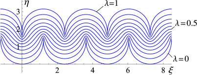
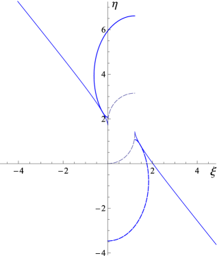
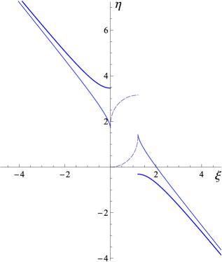
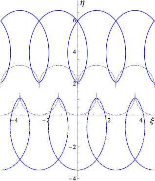
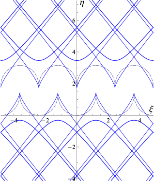
Now we consider the development of the extended oloid 𝒪𝒪\mathcal{O} onto its tangent plane E𝐸E. For this, we define a cartesian ξ,η𝜉𝜂\xi,\eta-coordinate system in E𝐸E as follows: Let E𝐸E touch 𝒪𝒪\mathcal{O} along the generating line

0={ω1(m,0),ω2(m,0),ω3(m,0)|m}subscript0conditional-setsubscript𝜔1𝑚0subscript𝜔2𝑚0subscript𝜔3𝑚0𝑚\mathcal{L}_{0}=\left\{\omega_{1}(m,0),\,\omega_{2}(m,0),\,-\omega_{3}(m,0)\>|\>m\in\mathbb{R}\right\}

(see (2) and the proof of Corollary 1). Then 0subscript0\mathcal{L}_{0} is the η𝜂\eta-axis, and the line perpendicular to 0subscript0\mathcal{L}_{0} in the point m=0𝑚0m=0 is the ξ𝜉\xi-axis.

Any curve 𝒞𝒪𝒞𝒪\mathcal{C}\subset\mathcal{O} is developed onto a plane curve 𝒞Esuperscript𝒞𝐸\mathcal{C}^{*}\subset E. A parametrization of 𝒞superscript𝒞\mathcal{C}^{*} with the arc length t𝑡t of the double circular arc 𝒞0subscript𝒞0\mathcal{C}_{0} as parameter can be obtained from the vector transformation in [2, p. 114, Theorem 4]. In the following for abbreviation we put c=cost𝑐𝑡c=\cos t, s=sint𝑠𝑡s=\sin t. \lfloor\cdot\rfloor denotes the integer part of \cdot .

Theorem 6.

The development of the touching curve 𝒞λsubscript𝒞𝜆\mathcal{C}_{\lambda} onto E𝐸E is the curve

𝒞λ={(κ1(λ,t),κ2(λ,t))|t}superscriptsubscript𝒞𝜆conditional-setsuperscriptsubscript𝜅1𝜆𝑡superscriptsubscript𝜅2𝜆𝑡𝑡\mathcal{C}_{\lambda}^{*}=\left\{(\kappa_{1}^{*}(\lambda,t),\,\kappa_{2}^{*}(\lambda,t))\>|\>t\in\mathbb{R}\right\}

with parametrization

κ1(λ,t)=superscriptsubscript𝜅1𝜆𝑡absent\displaystyle\kappa_{1}^{*}(\lambda,t)={} sgn(t)3|t|4π+124π33+sgn(h(t))κ~1(λ,h(t)),sgn𝑡3𝑡4𝜋124𝜋33sgn𝑡subscript~𝜅1𝜆𝑡\displaystyle\mathrm{sgn}(t)\cdot\left\lfloor\frac{3\,|t|}{4\pi}+\frac{1}{2}\right\rfloor\cdot\frac{4\pi}{3\,\sqrt{3}}+\mathrm{sgn}(h(t))\cdot\tilde{\kappa}_{1}(\lambda,h(t))\,,
κ2(λ,t)=superscriptsubscript𝜅2𝜆𝑡absent\displaystyle\kappa_{2}^{*}(\lambda,t)={} κ~2(λ,h(t)),subscript~𝜅2𝜆𝑡\displaystyle\tilde{\kappa}_{2}(\lambda,h(t))\,,

where

κ~1(λ,t)=subscript~𝜅1𝜆𝑡absent\displaystyle\tilde{\kappa}_{1}(\lambda,t)={} 239(arccos2c1+c+(12λ)|s|2(1+2c)(1+λc)1+c),2392𝑐1𝑐12𝜆𝑠212𝑐1𝜆𝑐1𝑐\displaystyle\frac{2\,\sqrt{3}}{9}\left(\arccos\frac{\sqrt{2}\,c}{\sqrt{1+c}}+\frac{(1-2\lambda)\left|s\right|\sqrt{2(1+2c)}}{(1+\lambda c)\,\sqrt{1+c}}\right),
κ~2(λ,t)=subscript~𝜅2𝜆𝑡absent\displaystyle\tilde{\kappa}_{2}(\lambda,t)={} 39(ln21+c+4+7λ+(11λ4)c1+λc),3921𝑐47𝜆11𝜆4𝑐1𝜆𝑐\displaystyle\frac{\sqrt{3}}{9}\left(\ln\frac{2}{1+c}+\frac{4+7\lambda+(11\lambda-4)c}{1+\lambda c}\right),
h(t)=𝑡absent\displaystyle h(t)={} tsgn(t)3|t|4π+124π3.𝑡sgn𝑡3𝑡4𝜋124𝜋3\displaystyle t-\mathrm{sgn}(t)\cdot\left\lfloor\frac{3\,|t|}{4\pi}+\frac{1}{2}\right\rfloor\cdot\frac{4\pi}{3}\,.
Proof.

Substituting x=κ1(λ,t)𝑥subscript𝜅1𝜆𝑡x=\kappa_{1}(\lambda,t), y=κ2(λ,t)𝑦subscript𝜅2𝜆𝑡y=\kappa_{2}(\lambda,t), z=κ3(λ,t)𝑧subscript𝜅3𝜆𝑡z=-\kappa_{3}(\lambda,t), see Corollary 1, in the vector transformation [2, p. 114, Theorem 4], a straight-forward calculation delivers

ξ=κ~~1(λ,t)=𝜉subscript~~𝜅1𝜆𝑡absent\displaystyle\xi=\tilde{\tilde{\kappa}}_{1}(\lambda,t)={} 239(arccos2c1+c+(12λ)s2(1+2c)(1+λc)1+c),2392𝑐1𝑐12𝜆𝑠212𝑐1𝜆𝑐1𝑐\displaystyle\frac{2\,\sqrt{3}}{9}\left(\arccos\frac{\sqrt{2}\,c}{\sqrt{1+c}}+\frac{(1-2\lambda)\,s\,\sqrt{2(1+2c)}}{(1+\lambda c)\,\sqrt{1+c}}\right),
η=κ~2(λ,t)=𝜂subscript~𝜅2𝜆𝑡absent\displaystyle\eta=\tilde{\kappa}_{2}(\lambda,t)={} 39(ln21+c+4+7λ+(11λ4)c1+λc).3921𝑐47𝜆11𝜆4𝑐1𝜆𝑐\displaystyle\frac{\sqrt{3}}{9}\left(\ln\frac{2}{1+c}+\frac{4+7\lambda+(11\lambda-4)c}{1+\lambda c}\right).

κ~2(λ,t)subscript~𝜅2𝜆𝑡\tilde{\kappa}_{2}(\lambda,t) is valid for tI1𝑡subscript𝐼1t\in I_{1} (see (3)). The periodic continuation of κ~2(λ,t)subscript~𝜅2𝜆𝑡\tilde{\kappa}_{2}(\lambda,t) yields κ2(λ,t)superscriptsubscript𝜅2𝜆𝑡\kappa_{2}^{*}(\lambda,t), valid for t𝑡t\in\mathbb{R}.

κ~~1(λ,t)subscript~~𝜅1𝜆𝑡\tilde{\tilde{\kappa}}_{1}(\lambda,t) is valid only for t[0,2π/3]𝑡02𝜋3t\in[0,2\pi/3]. The restriction of κ1(λ,t)superscriptsubscript𝜅1𝜆𝑡\kappa_{1}^{*}(\lambda,t) to tI1𝑡subscript𝐼1t\in I_{1} must be an odd function. Replacing sint𝑡\sin t by |sint|𝑡\left|\sin t\right| in κ~~1(λ,t)subscript~~𝜅1𝜆𝑡\tilde{\tilde{\kappa}}_{1}(\lambda,t), we get the even function κ~1(λ,t)subscript~𝜅1𝜆𝑡\tilde{\kappa}_{1}(\lambda,t), tI1𝑡subscript𝐼1t\in I_{1}. Now, κ1(λ,t):=sgn(t)κ~1(λ,t)assignsuperscriptsubscript𝜅1𝜆𝑡sgn𝑡subscript~𝜅1𝜆𝑡\kappa_{1}^{\diamond}(\lambda,t):=\mathrm{sgn}(t)\cdot\tilde{\kappa}_{1}(\lambda,t) is the required restriction of κ1(λ,t)superscriptsubscript𝜅1𝜆𝑡\kappa_{1}^{*}(\lambda,t). We get

κ1(λ,2π/3)κ1(λ,2π/3)=4π33,superscriptsubscript𝜅1𝜆2𝜋3superscriptsubscript𝜅1𝜆2𝜋34𝜋33\kappa_{1}^{\diamond}(\lambda,2\pi/3)-\kappa_{1}^{\diamond}(\lambda,-2\pi/3)=\frac{4\pi}{3\,\sqrt{3}}\,,

and therefore, using the step function

sgn(t)3|t|4π+124π33,sgn𝑡3𝑡4𝜋124𝜋33\mathrm{sgn}(t)\cdot\left\lfloor\frac{3\,|t|}{4\pi}+\frac{1}{2}\right\rfloor\cdot\frac{4\pi}{3\,\sqrt{3}}\,,

we have found κ1(λ,t)superscriptsubscript𝜅1𝜆𝑡\kappa_{1}^{*}(\lambda,t), valid for t𝑡t\in\mathbb{R}. ∎

For λ=0𝜆0\lambda=0 we have

κ~1(0,t)=subscript~𝜅10𝑡absent\displaystyle\tilde{\kappa}_{1}(0,t)={} 239(arccos2c1+c+|s|2(1+2c)1+c),2392𝑐1𝑐𝑠212𝑐1𝑐\displaystyle\frac{2\,\sqrt{3}}{9}\left(\arccos\frac{\sqrt{2}\,c}{\sqrt{1+c}}+\frac{\left|s\right|\sqrt{2(1+2c)}}{\sqrt{1+c}}\right),
κ~2(0,t)=subscript~𝜅20𝑡absent\displaystyle\tilde{\kappa}_{2}(0,t)={} 39(ln21+c+4(1c)).3921𝑐41𝑐\displaystyle\frac{\sqrt{3}}{9}\left(\ln\frac{2}{1+c}+4(1-c)\right).

The following manipulation of the second term in the brackets of κ~1(0,t)subscript~𝜅10𝑡\tilde{\kappa}_{1}(0,t),

|sint|2(1+2cost)1+cost=2|sint2||cost2|2(1+2cost)2cos2t2𝑡212𝑡1𝑡2𝑡2𝑡2212𝑡2superscript2𝑡2\displaystyle\frac{\left|\sin t\right|\sqrt{2(1+2\cos t)}}{\sqrt{1+\cos t}}=\frac{2\left|\sin\frac{t}{2}\right|\left|\cos\frac{t}{2}\right|\sqrt{2(1+2\cos t)}}{\sqrt{2\cos^{2}\frac{t}{2}}}
=2|sint2|2(1+2cost)=212(1cost)2(1+2cost)absent2𝑡2212𝑡2121𝑡212𝑡\displaystyle=\sqrt{2}\>\left|\sin\frac{t}{2}\right|\sqrt{2(1+2\cos t)}=\sqrt{2}\;\sqrt{\frac{1}{2}(1-\cos t)}\;\sqrt{2(1+2\cos t)}
=2(1+2cost)(1cost),absent212𝑡1𝑡\displaystyle=\sqrt{2(1+2\cos t)(1-\cos t)}\,,

shows that we have obtained the result of [2, p. 108, Theorem 2]. For λ=1𝜆1\lambda=1 we get

κ~1(1,t)=subscript~𝜅11𝑡absent\displaystyle\tilde{\kappa}_{1}(1,t)={} 239(arccos2c1+c|s|2(1+2c)(1+c)3/2),2392𝑐1𝑐𝑠212𝑐superscript1𝑐32\displaystyle\frac{2\,\sqrt{3}}{9}\left(\arccos\frac{\sqrt{2}\,c}{\sqrt{1+c}}-\frac{\left|s\right|\sqrt{2(1+2c)}}{(1+c)^{3/2}}\right),
κ~2(1,t)=subscript~𝜅21𝑡absent\displaystyle\tilde{\kappa}_{2}(1,t)={} 39(ln21+c+11+7c1+c).3921𝑐117𝑐1𝑐\displaystyle\frac{\sqrt{3}}{9}\left(\ln\frac{2}{1+c}+\frac{11+7c}{1+c}\right).

This is the result of [2, p. 112, Theorem 3]. For λ=1/2𝜆12\lambda=1/2 we have

κ~1(1/2,t)=subscript~𝜅112𝑡absent\displaystyle\tilde{\kappa}_{1}(1/2,t)={} 239arccos2c1+c,2392𝑐1𝑐\displaystyle\frac{2\,\sqrt{3}}{9}\arccos\frac{\sqrt{2}\,c}{\sqrt{1+c}}\,,
κ~2(1/2,t)=subscript~𝜅212𝑡absent\displaystyle\tilde{\kappa}_{2}(1/2,t)={} 39(ln21+c+3(5+c)2+c),3921𝑐35𝑐2𝑐\displaystyle\frac{\sqrt{3}}{9}\left(\ln\frac{2}{1+c}+\frac{3(5+c)}{2+c}\right),

which is the result of [2, p. 115]. Examples with λ[0,1]𝜆01\lambda\in[0,1] are shown in Fig. 9.

Refer to caption
Fig. 9: The curves 𝒞λsuperscriptsubscript𝒞𝜆\mathcal{C}_{\lambda}^{*}, λ=0, 0.1, 0.2,, 0.9, 1𝜆00.10.20.91\lambda=0,\,0.1,\,0.2,\ldots,\,0.9,\,1

For λ±𝜆plus-or-minus\lambda\rightarrow\pm\infty (see Fig. 11 and Fig. 13) one easily finds

limλ±κ~1(λ,t)=subscript𝜆plus-or-minussubscript~𝜅1𝜆𝑡absent\displaystyle\lim_{\lambda\rightarrow\pm\infty}\tilde{\kappa}_{1}(\lambda,t)={} 239(arccos2c1+c2|s|2(1+2c)c1+c),2392𝑐1𝑐2𝑠212𝑐𝑐1𝑐\displaystyle\frac{2\,\sqrt{3}}{9}\left(\arccos\frac{\sqrt{2}\,c}{\sqrt{1+c}}-\frac{2\left|s\right|\sqrt{2(1+2c)}}{c\,\sqrt{1+c}}\right),
limλ±κ~2(λ,t)=subscript𝜆plus-or-minussubscript~𝜅2𝜆𝑡absent\displaystyle\lim_{\lambda\rightarrow\pm\infty}\tilde{\kappa}_{2}(\lambda,t)={} 39(ln21+c+7+11cc).3921𝑐711𝑐𝑐\displaystyle\frac{\sqrt{3}}{9}\left(\ln\frac{2}{\sqrt{1+c}}+\frac{7+11c}{c}\right).

As further examples, the curves 𝒞0.5superscriptsubscript𝒞0.5\mathcal{C}_{-0.5}^{*} and 𝒞1.5superscriptsubscript𝒞1.5\mathcal{C}_{1.5}^{*} are shown in Fig. 11 and Fig. 13.
After substituting

x=g1(t)=𝑥subscript𝑔1𝑡absent\displaystyle x=g_{1}(t)={} sinttant3,y=g2(t)=2+3cost3cos2t2cos3t6(1+cost)cost,𝑡𝑡3𝑦subscript𝑔2𝑡23𝑡3superscript2𝑡2superscript3𝑡61𝑡𝑡\displaystyle\frac{\sin t-\tan t}{3}\,,\quad y=g_{2}(t)=\frac{2+3\cos t-3\cos^{2}t-2\cos^{3}t}{6(1+\cos t)\cos t}\,,
z=g3(t)=𝑧subscript𝑔3𝑡absent\displaystyle z=g_{3}(t)={} (1+2cost)3/23(1+cost)costsuperscript12𝑡3231𝑡𝑡\displaystyle-\frac{(1+2\cos t)^{3/2}}{3(1+\cos t)\cos t}

(see Theorem 2) in the vector transformation [2, p. 114, Theorem 4], analogous steps as in the proof of Theorem 6 result in the development superscript\mathcal{R}^{*} of the edge of regression \mathcal{R}. We state the result in the following theorem.

Theorem 7.

The development of \mathcal{R} onto E𝐸E is the curve

={(g1(t),g2(t))|t}superscriptconditional-setsuperscriptsubscript𝑔1𝑡superscriptsubscript𝑔2𝑡𝑡\mathcal{R}^{*}=\left\{(g_{1}^{*}(t),\,g_{2}^{*}(t))\>|\>t\in\mathbb{R}\right\}

with parametrization

g1(t)=superscriptsubscript𝑔1𝑡absent\displaystyle g_{1}^{*}(t)={} sgn(t)3|t|4π+124π33+sgn(h(t))g~1(h(t)),sgn𝑡3𝑡4𝜋124𝜋33sgn𝑡subscript~𝑔1𝑡\displaystyle\mathrm{sgn}(t)\cdot\left\lfloor\frac{3\,|t|}{4\pi}+\frac{1}{2}\right\rfloor\cdot\frac{4\pi}{3\,\sqrt{3}}+\mathrm{sgn}(h(t))\cdot\tilde{g}_{1}(h(t))\,,
g2(t)=superscriptsubscript𝑔2𝑡absent\displaystyle g_{2}^{*}(t)={} g~2(h(t)),subscript~𝑔2𝑡\displaystyle\tilde{g}_{2}(h(t))\,,

where

g~1(t)=subscript~𝑔1𝑡absent\displaystyle\tilde{g}_{1}(t)={} 239(arccos2c1+c(2+2cc2)2(1+2c)|s|3c(1+c)3/2),2392𝑐1𝑐22𝑐superscript𝑐2212𝑐𝑠3𝑐superscript1𝑐32\displaystyle\frac{2\,\sqrt{3}}{9}\left(\arccos\frac{\sqrt{2}\,c}{\sqrt{1+c}}-\frac{(2+2c-c^{2})\,\sqrt{2(1+2c)}\left|s\right|}{3c\,(1+c)^{3/2}}\right),
g~2(t)=subscript~𝑔2𝑡absent\displaystyle\tilde{g}_{2}(t)={} 39(ln21+c+7+33c+18c24c33c(1+c)).3921𝑐733𝑐18superscript𝑐24superscript𝑐33𝑐1𝑐\displaystyle\frac{\sqrt{3}}{9}\left(\ln\frac{2}{1+c}+\frac{7+33c+18c^{2}-4c^{3}}{3c\,(1+c)}\right).

superscript\mathcal{R}^{*} is shown in the Figures 11, 11, 13.

Refer to caption
Fig. 10: 𝒞0.5superscriptsubscript𝒞0.5\mathcal{C}_{-0.5}^{*} (thick, dashed), 𝒞1.5superscriptsubscript𝒞1.5\mathcal{C}_{1.5}^{*} (thick), superscript\mathcal{R}^{*} (thin), 𝒞0superscriptsubscript𝒞0\mathcal{C}_{0}^{*}, 𝒞1superscriptsubscript𝒞1\mathcal{C}_{1}^{*}; 0t2π/30𝑡2𝜋30\leq t\leq 2\pi/3
Refer to caption
Fig. 11: 𝒞±superscriptsubscript𝒞plus-or-minus\mathcal{C}_{\pm\infty}^{*} (thick), superscript\mathcal{R}^{*} (thin), 𝒞0superscriptsubscript𝒞0\mathcal{C}_{0}^{*} and 𝒞1superscriptsubscript𝒞1\mathcal{C}_{1}^{*} (dashed); 0t2π/30𝑡2𝜋30\leq t\leq 2\pi/3
Refer to caption
Fig. 12: 𝒞0.5superscriptsubscript𝒞0.5\mathcal{C}_{-0.5}^{*} (thick, dashed), 𝒞1.5superscriptsubscript𝒞1.5\mathcal{C}_{1.5}^{*} (thick), 𝒞0superscriptsubscript𝒞0\mathcal{C}_{0}^{*} and 𝒞1superscriptsubscript𝒞1\mathcal{C}_{1}^{*} (thin, dashed)
Refer to caption
Fig. 13: 𝒞±superscriptsubscript𝒞plus-or-minus\mathcal{C}_{\pm\infty}^{*} (thick), superscript\mathcal{R}^{*} (thin), 𝒞0superscriptsubscript𝒞0\mathcal{C}_{0}^{*} and 𝒞1superscriptsubscript𝒞1\mathcal{C}_{1}^{*} (dashed)

References

  • [1] E. Czuber: Vorlesungen über Differential- und Integralrechnung, B. G. Teubner, Leipzig 1912.
  • [2] H. Dirnböck, H. Stachel: The Development of the Oloid, JGG 1, No. 2 (1997), 105-118.
  • [3] K. Fladt, A. Baur: Analytische Geometrie spezieller Flächen und Raumkurven, Friedr. Vieweg & Sohn, Braunschweig 1975.
  • [4] K. Kommerell: Vorlesungen über analytische Geometrie des Raumes, Koehler & Amelang, Leipzig 1953.
  • [5] K. Rohn, E. Papperitz: Lehrbuch der darstellenden Geometrie, Bd. 3, 3. Aufl., Veit & Comp., Leipzig 1906.
  • [6] D. M. Y. Sommerville: Analytical Geometry of Three Dimensions, Cambridge University Press, Cambridge 1939.
  • [7] K. Strubecker: Differentialgeometrie I, Sammlung Göschen Bd. 1113/ 1113 a, Walter de Gruyter & Co., Berlin 1955.
  • [8] http:/​/de.wikipedia.org/wiki/Oloid, 12.02.2015;
    http:/​/en.wikipedia.org/wiki/Oloid, 12.02.2015

Uwe Bäsel Hans Dirnböck
HTWK Leipzig, Fakultät Nussberg 22
Maschinenbau und Energietechnik, 9062 Moosburg, Austria
Karl-Liebknecht-Straße 134,
04277 Leipzig, Germany
uwe.baesel@htwk-leipzig.de