Numerical and experimental study of the effects of noise on the permutation entropy

Abstract

We analyze the effects of noise on the permutation entropy of dynamical systems. We take as numerical examples the logistic map and the Rössler system. Upon varying the noise strengthfaster, we find a transition from an almost-deterministic regime, where the permutation entropy grows slower than linearly with the pattern dimension, to a noise-dominated regime, where the permutation entropy grows faster than linearly with the pattern dimension. We perform the same analysis on experimental time-series by considering the stochastic spiking output of a semiconductor laser with optical feedback. Because of the experimental conditions, the dynamics is found to be always in the noise-dominated regime. Nevertheless, the analysis allows to detect regularities of the underlying dynamics. By comparing the results of these three different examples, we discuss the possibility of determining from a time series whether the underlying dynamics is dominated by noise or not.

Keywords: Time series analysis, Entropy, Ordinal patterns, Permutation entropy, Stochastic systems, Symbolic analysis.

1 Introduction

Ordinal analysis is a method of time series analysis that consists of computing the probabilities of ordinal patterns, which are defined according to the ordering of $D$ consecutive values in the series [1]. The entropy of these probabilities, referred to as permutation entropy, is a tool to detect possible regularities in the time series. In recent years, ordinal patterns and permutation entropy have been widely used to investigate complex dynamical systems [2, 3]. They have been employed in the attempt to distinguish noise from chaos [4, 5, 6, 7], to detect noise-induced order [8], serial correlations [9] and dependencies between two or more time series [10, 11, 12, 13, 16, 14, 15], among many other examples. Applications to experimental time series analysis include classification and discrimination of dynamical states in normal and epileptic EEG [17, 18, 19, 20] and detection of heart rate variability under different physiological and pathological conditions [21, 22, 23].

Given this growing interest, it is relevant to understand the relation between the permutation entropy and other complexity measures. In particular, a well-established way to characterize the production of information of a dynamical system is the Kolmogorov-Sinai entropy $h_{ks}$, see e.g. [24, 25]. To compute $h_{ks}$, the time series is discretized by partitioning the phase space into regions and assigning a symbol to each region. Then one computes the probabilities of blocks, which are vectors of $D$ consecutive symbols (more details in the following sections). The entropy of the block probabilities is the block entropy. The Kolmogorov-Sinai entropy is finally obtained as the rate of growth, for $D\rightarrow\infty$ and in the limit of a very refined partition, of the block entropy.

Similarly to $h_{ks}$, one can introduce a permutation entropy rate as the rate of growth for $D\rightarrow\infty$ of the permutation entropy. Both the permutation entropy and the Kolmogorov-Sinai entropy measure the “asymptotic” information rate of representations of the time series, the former with ordinal patterns (based in the relative order of consecutive values) and the latter with blocks (based on a partition of the phase space). The permutation entropy rate and $h_{ks}$ are not only conceptually related: for piecewise monotone interval maps on the real line, they were shown to be equal [26]. This result has been later extended to a broad class of dynamics [27, 28]. This equivalence is non-trivial considering, for example, that the number of total possible ordinal patterns grows with $D$ as $D!$, while the number of blocks grows as $Q^{D}$ where $Q$ is the total number of symbols. The two quantities can be equal only thanks to the large number of forbidden ordinal patterns, strongly limiting the growth of the permutation entropy as $D$ is increased.

These mathematical results clarify that, under general hypotheses, permutation and block entropies share the same asymptotic behavior. However, due to difficulties in reaching the asymptotic regime, this equivalence can be of little use in many practical cases. For example, it has been noted [26] that the rate of convergence of the permutation entropy to the Kolmogorov-Sinai entropy is extremely slow even for one-dimensional maps, while on the contrary, block entropies converge very quickly, see e.g. [24].

Comparing the two analyses becomes even more problematic for high-dimensional and/or noisy dynamics, such as typical experimental time-series. Consider for example the extreme case of a time series dominated by noise, in which all symbols are equally probable and temporal correlations are absent. In this case, the block entropy of length $D$ is equal to $D\ln(Q)$, where $Q$ is the total number of symbols, while the permutation entropy with patterns of length $D$ is equal to $\ln(D!)\sim D\ln D$. This means that the block entropy is linear in $D$, with a slope $\ln(Q)$, explicitly dependent on the chosen partition, which diverges only in the limit of a very refined partition, $Q\rightarrow\infty$. In contrast, the permutation entropy grows more than linearly, so that their asymptotic slope is infinite. In both cases, the result is an infinite entropy rate. However, to discover it, in the first case one needs to construct a very refined partition. In the second case, one needs to reach large values of $D$ to appreciate that the slope increases logarithmically. Both these tasks can be very difficult when analyzing a finite time series due to statistical limitations.

Our goal is to get a better understanding of how noise influences the permutation entropy. To this aim, we analyze simulated and experimental time series. We mostly focus on permutation entropy as the effect of noise on block entropies is fairly well understood, see e.g. [29, 30]. We first analyze time series generated from the logistic map and from Poincaré sections of the three-dimensional Rössler system. We conclude with an experimental example of output intensity data recorded from a semiconductor laser with optical feedback.

2 Methods

2.1 Numerical data

We consider two dynamical systems: the one-dimensional logistic map and the three-dimensional Rössler system. In both cases, we study the effect of adding to the dynamical equations a Gaussian white noise, $\xi_{t}$ with $\langle\xi_{t}\rangle=0$ and temporal correlation $\langle\xi_{t}\xi_{t^{\prime}}\rangle=\delta_{t,t^{\prime}}$. We considered also the case of observational noise (not shown), where the dynamics is deterministic but the noise affects the observation, obtaining very similar results.

2.1.1 Logistic map

$$x_{t+1}=4x_{t}(1-x_{t})+\alpha\xi_{t},$$ (1)

where $x_{t}$ is the state of the system at iteration $t$ and $\alpha$ is the noise strength. In order to constrain the variable $x_{t}$ in the interval $[0,1]$, the values of $\xi_{t}$ that would lead to $x_{t+1}>1$ or $x_{t+1}<0$ are simply discarded and redrawn. Thus, the noise $\xi_{t}$ is temporally uncorrelated, but not purely Gaussian due to this truncation effect. To investigate the variation of the permutation entropy with the noise strength, we computed the permutation entropy, for each value of $\alpha$, from time series of length $N=12\times 10^{7}$. We have also studied other nonlinear one-dimensional maps (Tent, Bernoulli and Quadratic) and obtained very similar results to those of the logistic map (results not shown).

2.1.2 Rössler system

The Rössler equations read

$$\dot{X} = -Y-Z+\alpha\xi(t),$$

$$\dot{Y} = X+aY$$ (2)

$$\dot{Z} = b+Z(X-c)$$

where $\{X,Y,Z\}$ are the states of the system at time $t$, $\alpha$ is the noise strength and $\{a,b,c\}$ are the local parameters set at {$0.1,\,0.1,\,18.0$}, respectively.

In order to apply the symbolic methods (ordinal patterns or blocks) we need to discretize the dynamics. Instead of employing temporal sampling [32], we introduce a Poincaré section [33] at $X=0$, and analyze the time intervals between consecutive crossings of the Poincaré plane. For each value of $\alpha$, the permutation entropy is computed from time-series of $N=12\times 10^{7}$ data points.

2.2 Experimental data

Experimental data was recorded from the output intensity of a semiconductor laser with optical feedback operating in the low-frequency fluctuations (LFFs) regime. In this regime, the laser intensity displays sudden and apparently random dropouts, followed by gradual recoveries. This spiking dynamics has received considerable attention because the intensity dropouts are induced by stochastic effects and deterministic nonlinearities. The optical feedback introduces a delay which renders the system in principle infinite dimensional. Therefore, the laser in the LFF regime generates complex fluctuations that, because of the stochastic and high-dimensional nature of the underlying dynamics, are suitable to be investigated by means of complexity measures such as the permutation and block entropies.

The experimental setup is the same as in [31] and uses a 650 nm AlGaInP semiconductor laser (SONY SLD1137VS) with optical feedback. The feedback was given through a mirror placed 70 cm apart from the laser cavity, with a round trip of 4.7 ns. The feedback was controlled using a neutral density filter that can adjusts the light intensity injected into the laser. The laser has a solitary threshold current of $I_{th}=28.4$ mA. The temperature and current of the laser were stabilized using a combi controller Thorlabs ITC501 with an accuracy of $0.01$ C and $0.01$ mA, respectively. The current used during the experiment was $I=29.3$ mA and the temperature was set at $T=17$ C. The neutral density filter was adjusted so that the threshold reduction due to feedback was about 7%. The signal was captured using a photo detector (Thorlabs DET210) connected to a FEMTO HSA-Y-2-40 amplifier and registered with a 1 GHz digital oscilloscope (Agilent Infiniium DSO9104A) with $0.2$ ns of sampling. The intensity time series were acquired from the oscilloscope by a LabVIEW program that uses a threshold to detect the times when the intensity drops, and calculates the time intervals between successive threshold crossings (in the following, referred to as inter-dropout-intervals, IDIs). We recorded in this way time series of more than $10^{5}$ consecutive IDIs.

2.3 Methods of analysis

We compare two different methods to transform a time-series, $x(t)=\{x(1)$, $x(2)\dots x(N)\}$, into a sequence of symbols, $s(t)$: ordinal patterns and blocks.

In both cases, one needs to choose a dimension $D$ for defining vectors made up of consecutive entries of the time series, i.e. $\{x(i),x(i+1),\dots,x(i+D-1)\}$. Ordinal patterns and blocks differ by the way in which the entries of these vectors are transformed into symbols. Ordinal patterns classify them according to the ranking (from the largest to the smallest value) of the $D$ entries in the vectors. The total number of ordinal patterns of length $D$ is then equal to the number of permutations, $D!$. For example, with $D=2$ there are two ordinal patterns: $x(t_{i})>x(t_{i+1})$ corresponding to the ordinal pattern ‘$01$’ and $x(t_{i})<x(t_{i+1})$ corresponding to the ordinal pattern ‘$10$’.

For blocks, the phase space is first divided into $Q$ regions, associating a symbol to each region. Blocks represent all vectors in which each value of the time series correspond to the same symbol. For example, let us consider the time series $x(t)=\{0.1,0.6,0.7,0.3\}$, and partition the phase space into the two regions $[0,0.5)$ and $[0.5,1]$, associating to them the symbols $0$ and $1$ respectively. With $D=2$, the blocks associated to the time series are $\{01,11,10\}$.

Then, the permutation entropy [1] or the block entropy [24, 25] are simply the entropy of the frequency $p_{i}$ of the different patterns in the time series

$$H_{D}=-\sum_{i}^{M}p_{i}\ln p_{i},$$ (3)

where $M$ is the number of possible patterns: for permutation entropy, $M=D!$, while for block entropy, $M=Q^{D}$.

3 Results

Figure 1: Permutation entropy ($H$) as a function of the size of the ordinal pattern ($D$) and the noise strength ($\alpha$) for data generated from the Logistic map. (a) $H$ vs $D$ for $\alpha=1\times 10^{-4}$ (stars), $\alpha=2\times 10^{-2}$ (triangles), $\alpha=5\times 10^{-2}$ (inverted triangles), $\alpha=0.1$ (circles), $\alpha=$1 (pentagons) and $H_{max}=\ln D!$ (solid line). (b) $H$ versus $\alpha$ for $D=2$ (stars), $D=3$ (triangles), $D=4$ (inverted triangles), $D=5$ (circles), $D=6$ (pentagons), $D=7$ (squares) and $D=8$ (diamonds).

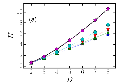
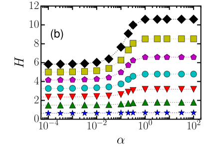
Figure 1a displays the permutation entropy, $H$, vs the dimension of the ordinal patterns, $D$, computed from time series of the logistic map at different noise strengths. It can be observed that $H$ increases monotonically with $D$, regardless of the noise strength. As the noise increases, $H$ approaches its maximum value, corresponding to equally probable ordinal patterns, $H_{max}=\ln D!$ (solid black line). Note that at ${\alpha=1}$ (pentagons) the values of $H$ is already very close to $H_{max}$. Figure 1b displays $H$ as a function of the noise strength $\alpha$. A clear transition from low-noise to high-noise can be observed, for a value of the noise strength approximately independent of $D$. The difference between the values of the entropies at low and high noise becomes more pronounced as $D$ increases.

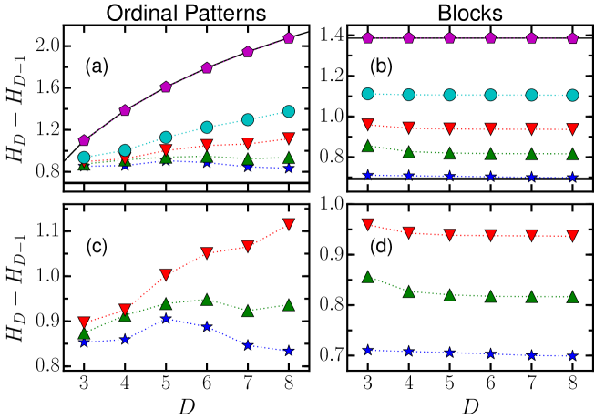
To further investigate this transition, Fig. (2a) displays the difference $H_{D}-H_{D-1}$ as a function of $D$, for various values of noise strength. As before, we indicate with a thin black line the noise-dominated limit in which all patterns are equiprobable, $H_{D}-H_{D-1}=(\ln D!-\ln(D-1)!)$. In the opposite limit of almost-deterministic, as $D$ grows the expected value of $H_{D}-H_{D-1}$ is the Kolmogorov-Sinai entropy [26], which for a one-dimensional chaotic map is equal to the Lyapunov exponent $\lambda$. In the case of logistic map for a local parameter set at $4$ one has $\lambda=\ln 2$, indicated by the thick black line. As shown in detail in Fig. (2c), we identify three possibilities:

• a almost-deterministic regime in which $H_{D}-H_{D-1}$ decreases for large $D$,

• a noise-dominated regime in which $H_{D}-H_{D-1}$ increases for large $D$,

• an intermediate regime in which $H_{D}-H_{D-1}$ remains nearly constant with $D$.

Figure 2: Comparison of the entropy computed from ordinal patterns, and the entropy computed from the blocks, for the Logistic map. The difference $H_{D}-H_{D-1}$ is plotted vs. the dimension of the ordinal patterns (a,c) and of the blocks (b,d) for various values of noise strength [the noise strengths are as in Fig. (1a)]. In panels (a) and (b) the solid lines indicate the asymptotic values for low noise (thick) and high noise (thin). Panel (c) and (d) display a detail of (a) and (b).

In principle, this qualitative feature of the permutation entropy can be applied to experimental time series to assess whether the dynamics is dominated by noise or by the deterministic dynamics.

We remind that this distinction can not be done for the block entropy, as in this case $H_{D}-H_{D-1}$ is necessarily a decreasing function of $D$ (see e.g. [34, 35]). This fundamental difference between permutation entropy and block entropy can be appreciated by comparing the left and right panels of Fig. (2).

For the analysis of the Rossler data, we considered the Poincaré map $X=0$, shown in Fig. (3a), and analyzed the sequence of time-intervals between consecutive crossings. Figure (3b) shows the difference $H_{D}-H_{D-1}$ vs $D$, for different values of $\alpha$. The solid line indicates the expected value if all ordinal patterns were equally probable, $H_{D}-H_{D-1}=\ln D!-\ln(D-1)!$. Because of the high level of stochasticity, we calculate the confidence interval that is consistent with the null hypothesis of equally probable ordinal patterns: in Fig. (3b) the gray region represents the expected value $\pm 3\sigma$, where $\sigma$ is the standard deviation calculated for a hundred surrogated (shuffle) time-series.

Figure 3: (a) Rössler attractor and Poincaré section in $X=0$. (b) Permutation entropy difference, $H_{D}-H_{D-1}$, vs the dimension of the ordinal patterns, $D$, for noise strength $\alpha=[0$ (star), $0.8$ (triangle), $1.6$ (inverted triangle), $2.4$ (circle), $3.2$ (pentagon), $4$ (square)$]$. The gray region indicates the values of $H_{D}-H_{D-1}$ that are consistent with equally probable ordinal patterns (see text for details). For the smallest value of alpha, $H_{D}-H_{D-1}$ shows a non-monotonic behavior, while for higher values of the noise strength, $H_{D}-H_{D-1}$ grows monotonically with $D$.

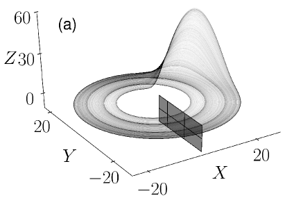
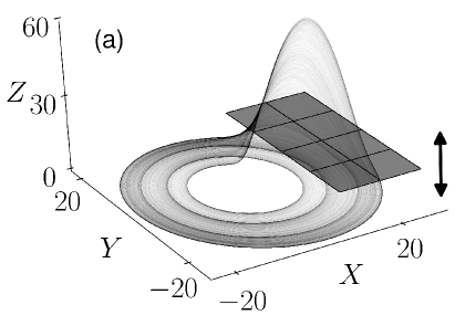
Before testing the method in experimental data we want to investigate how the choice of the Poincaré section influences the results. We consider a Poincaré section in the plane $Z=\beta$, as shown in Fig. (4a), and varying $\beta$ in the range $[0.05-26.7]$, for a fixed value of $\alpha=0$. In this case, to discretize the time series, we analyze the time values when the trajectory intersects the Poincaré section and $Z$ grows.

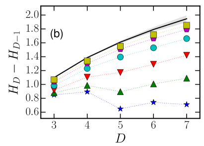
Figure (4b) displays the difference $H_{D}-H_{D-1}$ vs. $D$, for different values of $\beta$. We can see that the difference $H_{D}-H_{D-1}$ increases with $\beta$. This is due to the fact that, as $\beta$ is increased, consecutive values in the time-series become increasingly uncorrelated, similarly to when increasing the noise strength. On the contrary, for the minimum value of $\beta$, the variation of $H_{D}-H_{D-1}$ with $D$ is resemblant to the behavior under almost-deterministic observed in Fig. (3b).

Figure 4: (a) Rössler attractor and Poincaré section placed in $z=\beta$. (b) Permutation entropy difference, $H_{D}-H_{D-1}$, vs the dimension of the ordinal patterns, $D$, for $\beta=0.05$ (stars), $\beta=6.7$ (triangles), $\beta=13.4$ (inverted triangles), $\beta=20.0$(circles), $\beta=26.7$ (pentagons). The behavior is qualitatively similar to the one observed in Fig. (3b).

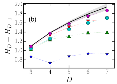
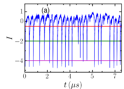
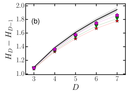
Finally, we analyze experimental data from the laser output intensity, displayed in Fig. (5a). To discretize the data we consider the thresholds indicated with horizontal lines in Fig. (5a), and analyzed the time intervals between consecutive threshold-crossings [9, 7, 31]. Figure (5b) displays the difference $H_{D}-H_{D-1}$ vs. $D$, for different thresholds. Note that $H_{D}-H_{D-1}$ varies with the threshold in a similar way as in Fig. (4b): as the threshold decreases, correlations between consecutive dropouts are lost.

For all the thresholds, $H_{D}-H_{D-1}$ grows monotonically with $D$. The reason is that the empirical time series is very noisy and the “almost-deterministic” regime is not seen, not even for the highest threshold. Nevertheless, the values of $H_{D}-H_{D-1}$ lie outside the gray region that indicates values consistent with equally probable ordinal patterns. This reveals that the sequence of intensity dropouts are not completely uncorrelated, and thus, this method can determine regularities also in very noisy data.

Figure 5: (a) Experimentally recorded time-series for the output intensity of a semiconductor laser, which operates in the low-frequency fluctuations (LFFs) regime, induced by self time-delayed optical feedback. The horizontal lines indicate the thresholds used to detect the dropout times. (b) Permutation entropy difference, $H_{D}-H_{D-1}$, vs the dimension of the ordinal patterns, for different thresholds: $-0.5$ (stars), $-2$ (inverted triangles) and $-4$ (pentagons).

4 Conclusion

We have studied the influence of noise in the permutation entropy of dynamical systems, considering both, simulated data and experimental data. In the simulated data, when increasing the noise strength, a transition between a almost-deterministic regime and a noise-dominated regime was clearly observed. The noise value at which this transition occurs is roughly independent of the size $D$ of the ordinal pattern.

In the almost-deterministic regime, the permutation entropy grows almost linearly or sub-linearly with $D$. This behavior is qualitatively similar to that of the block entropy. However, to observe a quantitative equivalence it is often needed to analyze extremely long time series, which can be computationally unfeasible even for relatively simple dynamical systems. In the noise-dominated regime, the growth is faster than linear, i.e. the differences $H_{D}-H_{D-1}$ increase with $D$. In principle, this fact can be used to determine whether the dynamics is in a noise-dominated or a almost-deterministic regime from an experimental time series where the noise strength can not be externally tuned. However, care must be taken in interpreting the results, as extracting a one-dimensional time series from a purely deterministic high-dimensional time series via a Poincaré map can lead to ordinal patterns which look effectively noisy, as we demonstrated in the example of the Rössler systems. This fact reflects the well-known difficulties of distinguishing deterministic dynamics from noise when dealing with high-dimensional systems [29].

5 Acknowledge

This work was supported by grants EOARD FA9550-14-1-0359, Ministerio de Ciencia e Innovacion, Spain and FEDER, FIS2012-37655-C02-01 and the Marie Curie Initial Training Network NETT, FP7-PEOPLE-2011-ITN 289146.

References

- [1] C. Bandt and B. Pompe, Phys. Rev. Lett. 88, 174102 (2002).
- [2] Zanin, M., Zunino, M., Rosso, O. A. and Papo, D. Entropy 14, 1553 (2012).
- [3] Amigó, J. M., Keller, K. and Kurths, J. Eur. Phys. J. Spec. Top. 222, 2 (2013).
- [4] J. M. Amigó, L. Kocarev, and J. Szczepanski, Phys. Rev. A 355, 27 (2006).
- [5] O. A. Rosso, H. A. Larrondo, M. T. Martin, A. Plastino, and M. A. Fuentes, Phys. Rev. Lett. 99, 154102 (2007).
- [6] J. M. Amigó, S. Zambrano, and M. A. Sanjuán, Europhys Lett. 83, 60005 (2008).
- [7] A. Aragoneses, N. Rubido, J. Tiana-Alsina, M. C. Torrent, and C. Masoller, Sci. Rep. 3, 1778 (2013).
- [8] O. A. Rosso and C. Masoller, Phys. Rev. E 79, 040106 (2009).
- [9] J. Tiana-Alsina, M. C. Torrent, O. A. Rosso, C. Masoller, and J. Garcia-Ojalvo, Phys. Rev. A 82, 013819 (2010).
- [10] Groth, A. Visualization of coupling in time series by order recurrence plots. Phys. Rev. E 72, 046220 (2005).
- [11] J. S. Cánovas, A. Guillamón, and M. d. C. Ruíz, Physica D 240, 1199 (2011).
- [12] A. Bahraminasab, F. Ghasemi, A. Stefanovska, P. V. McClintock, and H. Kantz, Phys. Rev. Lett. 100, 084101 (2008).
- [13] M. Matilla-García and M. R. Marín, Geogr. Anal. 43, 228 (2011).
- [14] P. M. Saco, L. C. Carpi, A. Figliola, E. Serrano, and O. A. Rosso, Physica A 389, 5022 (2010).
- [15] M. Barreiro, A. C. Marti, and C. Masoller, Chaos 21, 013101 (2011).
- [16] M. Matilla-García and M. Ruiz Marín, J. Econometrics 144, 139 (2008).
- [17] N. Nicolaou and J. Georgiou, Expert Syst. Appl. 39, 202 (2012).
- [18] I. Veisi, N. Pariz, and A. Karimpour, Fast and Robust Detection of Epilepsy in Noisy EEG Signals Using Permutation Entropy, in Bioinformatics and Bioengineering, Proceedings of the 7th IEEE International Conference on, p. 200, 2007.
- [19] X. Li, G. Ouyang, and D. A. Richards, Epilepsy Res. 77, 70 (2007).
- [20] A. Bruzzo, B. Gesierich, M. Santi, C. A. Tassinari, N. Birbaumer, and G. Rubboli, Neurol. Sci. 29, 3 (2008).
- [21] U. Parlitz, S. Berg, S. Luther, A. Schirdewan, J. Kurths, and N. Wessel, Comput. Biol. Med. 42, 319 (2012).
- [22] B. Frank, B. Pompe, U. Schneider, and D. Hoyer, Med. Biol. Eng. Comput. 44, 179 (2006).
- [23] S. Berg, S. Luther, S. E. Lehnart, K. Hellenkamp, R. Bauernschmitt, J. Kurths, N. Wessel, and U. Parlitz, Comparison of features characterizing beat-to-beat time series, in International Biosignal Processing Conference, Proceedings of the, volume 49, p. 1, 2010.
- [24] C. Beck and F. Schögl. Thermodynamics of chaotic systems: an introduction. No. 4. Cambridge University Press, (1995).
- [25] G. Boffetta, M. Cencini, M. Falcioni, A. Vulpiani. Phys. Rep., 356, 367-474 (2002).
- [26] C. Bandt, G. Keller, and B. Pompe, Nonlineatity 15, 1595 (2002).
- [27] J. M. Amigó, M. B. Kennel, and L. Kocarev, Physica D 210, 77 (2005)
- [28] J. M. Amigó, Physica D 241, 789 (2012).
- [29] M. Cencini, M. Falcioni, E. Olbrich, H. Kanz, and A. Vulpiani, Phys. Rev. E 62, 427 (2000)
- [30] M. Falcioni, A. Vulpiani, G. Mantica and S. Pigolotti, Phys. Rev. Lett. 91, 044101 (2003).
- [31] T. Sorrentino, C. Quintero-Quiroz, A. Aragoneses, M. C. Torrent, and C. Masoller, Opt. Express 23, 5571 (2015).
- [32] L. De Micco, J. G. Fernández, H. A. Larrondo, A. Plastino, and O. A. Rosso, Physica A 391, 2564 (2012).
- [33] C. S. Daw, C. E. A. Finney, and E. R. Tracy, Rev. Sci. Instrum. 74, 915 (2003).
- [34] C. Shannon, Bell Syst. Tech. J. 27, 379 (1948).
- [35] A. Kolmogorov, IRE Trans. Information Theory 2, 102 (1956).